Weak convergence of particle swarm optimization

Abstract

Particle swarm optimization algorithm is a stochastic meta-heuristic solving global optimization problems appreciated for its efficiency and simplicity. It consists in a swarm of interacting particles exploring a domain and searching a global optimum. The trajectory of the particles has been well-studied in a deterministic case. More recently authors shed some light on the stochastic approach to PSO, considering particles as random variables and studying them with probabilistic and statistical tools. These works paved the way to the present article. We focus here on weak convergence, the kind of stochastic convergence that appears in the Central Limit Theorem. We obtain three main results related to three different frameworks. These three settings depend either on the regime of the particles (oscillation or fast convergence) or on the sampling strategy (along the trajectory or in the swarm). The main application of these results is the construction of confidence intervals around the local optimum found by the swarm. The theorems are illustrated by a simulation study.

1 Introduction

Eberhart and Kennedy (1995) introduced the particle swarm optimization algorithm (PSO) based on social interactions (behaviors of birds). Since then PSO has known a great popularity in many domains and gave birth to many variants of the original algorithm (see Zhang et al. 2015 for a survey of variants and applications). PSO is a stochastic meta heuristic solving an optimization problem without any evaluation of the gradient. The algorithm explores the search space in an intelligent way thanks to a population of particles interacting with each other and updated at each step their position and their velocity. The dynamic of the particles relies on two attractors: their personal best position (historical best position of the particle denoted $p_{n}^{s}$ below), and the neighborhood best position (corresponding to the social component of the particles, denoted $g_{n}^{s}$ ). In the dynamic equation, the attractors are linked with a stochastic process in order to explore the search space. Algorithm 1 refers to the classical version of PSO with $S$ particles and $N$ iterations.

Initialize the swarm of $S$ particles with random positions $x_{0}^{s}$ and velocities $v_{0}^{s}$ over the search space.

for $n=1$ to $N$ do

     Evaluate the optimization fitness function for each particle.

     Update $p^{s}_{n}$ (personal best position) and $g^{s}_{n}$ (neighborhood best position).

     Change velocity ($v_{n}^{s}$) and position ($x_{n}^{s}$) according to the dynamic equation.

end for

Algorithm 1 Classical PSO

The convergence and stability analysis of PSO are important matters. In the literature, there are two kinds of convergence:

• the convergence of the particles towards a local or global optimum. This convergence is not obtained with the classical version of PSO. Van den Bergh and Engelbrecht (2010) and Schmitt and Wanka (2015) proposed a modified version of PSO to obtain the convergence.

• the convergence of each particle to a point (e.g. Poli 2009).

If we focus on the convergence of each particle to a point, a prerequisite is the stability of the trajectory of the particles. In a deterministic case, Clerc and Kennedy (2002) dealt with the stability of the particles with some conditions on the parametrization of PSO. Later, Kadirkamanathan et al. (2006) used the Lyapunov stability theorem to study the stability. About the convergence of PSO, Van Den Bergh and Engelbrecht (2006) looked at the trajectories of the particles and proved that each particle converges to a stable point (deterministic analysis). Under stagnation hypotheses (no improvement of the personal and neighborhood best positions), Poli (2009) gives the exact formula of the second moment. More recently, Bonyadi and Michalewicz (2016) or Cleghorn and Engelbrecht (2018) provided results for the order-1 and order-2 stabilities with respectively stagnant and non-stagnant distribution assumptions (both weaker than the stagnation hypotheses).

Let us introduce some notations. We consider here a cost function $f:\mathbb{R}^{d}\rightarrow\mathbb{R}^{+}$ that should be minimized on a compact set $\mathrm{\Omega}$. Consequently the particles evolve in $\mathrm{\Omega}\subset\mathbb{R}^{d}$.

Let $x_{n}^{s}\in\mathbb{R}^{d}$ $1\leq s\leq S$ denote the position of particle number $s$ in the swarm at step $n$. Let $\left(r_{j,n}\right)_{j=1,...,n\geq 1}$ be sequences of independent random vectors in $\mathbb{R}^{d}$ whose margins obey a uniform distribution over $\left[0,1\right]$ and denote by $\omega,$ $c_{1}$ and $c_{2}$ three positive constants which will be discussed later. Then the PSO algorithm considered in the sequel is defined by the two following equations (or dynamic equation, Poli 2009):

$$\left\{\begin{aligned} v_{n+1}^{s}&=\omega\cdot v_{n}^{s}+c_{1}r_{1,n}\odot\left(p_{n}^{s}-x_{n}^{s}\right)+c_{2}r_{2,n}\odot\left(g_{n}^{s}-x_{n}^{s}\right),\\ x_{n+1}^{s}&=x_{n}^{s}+v_{n+1}^{s}.\\ \end{aligned}\right.$$ (1)

where $\odot$ stands for the Hadamard product:

$$u\odot v=\left(u_{1}v_{1},...,u_{d}v_{d}\right).$$

and $p_{n}^{s}$ (resp. $g_{n}^{s}$) is the best personal position (resp. the best neighborhood position of the particle $s$) :

$$p_{n}^{s} =\operatorname*{\arg\!\min}_{t\in\{x_{0}^{s},\ldots,x_{n}^{s}\}}f\left(t\right),$$

$$g_{n}^{s} =\operatorname*{\arg\!\min}_{t\in\{p_{n}^{s^{\prime}}:s^{\prime}\in\mathcal{V}(s)\}}f\left(t\right).$$

with $\mathcal{V}(s)$ the neighborhood of particle $s$. This neighborhood depends on the swarm’s topology: if the topology is called global (all the particles communicate between each other) then $g_{n}^{s}=g_{n}=\operatorname*{\arg\!\min}_{t\in\{p_{n}^{1},\ldots,p_{n}^{S}\}}f\left(t\right)$ (see (Lane et al., 2008)).

Our main objective is to provide (asymptotic) confidence sets for the global or local optimum of the cost function $f$. If $g=\operatorname*{\arg\!\min}_{t\in\mathrm{\Omega}}f\left(t\right)$ for some domain $\mathrm{\Omega}$, a confidence region for $g$ is a random set $\Lambda$ such that :

$$\mathbb{P}\left(g\in\Lambda\right)\geq 1-\alpha$$

for some small $\alpha\in\left(0,1\right)$. The set $\Lambda$ depends on the swarm and is consequently random due to the random evolution of the particles. The probability symbol above, $\mathbb{P}$, depends on the distribution of the particles in the swarm. Let us illustrate the use of confidence interval for a real-valued PSO. Typically the kind of results we expect is: $g\in\left[m,M\right]$ with a probability larger than, say .99 %. This does not aim at yielding a precise estimate for $g$ but defines a “control area” for $g$, as well as a measure of the imprecision and variability of PSO.

Convergence of the swarm will not be an issue here. In fact we assume that the personal and global best converge : see assumptions $\mathbf{A_{2}}$ and $\mathbf{B_{3}}$ below. We are interested in the “step after” : localizing the limit of the particles with high probability, whatever their initialization and trajectories.

Formally, confidence set estimation forces us to inspect order two terms (i.e. the rate of convergence), typically convergence of the empirical variance. The word asymptotic just means that the sample size increases to infinity.

The outline of the paper is the following. In the next section the three main results are introduced. They are all related to weak convergence of random variables and vectors (see (Billingsley, 1999) for a classical monograph) and obtained under three different sets of assumptions.

The two first consider the trajectory of single particles. The sample consists in the path of a fixed particle. We show that two different regimes should be investigated depending on the limiting behavior of $p_{n}$ and $g_{n}$. Briefly speaking : if the limits of $p_{n}$ and $g_{n}$ are distinct, the particles oscillate between them (which is a well-known characteristics of PSO), if the limits of $p_{n}$ and $g_{n}$ coincide, then particles converge at a fast, exponential, rate.

In the oscillating case a classical Central Limit Theorem is obtained relying essentially on martingale difference techniques. In the non-oscillating situation, the particle converges quickly and we have to use random matrices products to obtain a non-standard CLT. As by-products of these two subsections we will retrieve confidence sets of the form $\Lambda\left(x_{1}^{s}\ldots x_{n}^{s}\right)$, depending on the $n$ positions of each particle $x^{s}$.

The third result states another classical CLT. The sample consists here in the whole swarm. This time the confidence set is of the form $\Lambda\left(x_{n}^{1}\ldots x_{n}^{S}\right)$, depending on the $S$ particles of the swarm when the iteration step is fixed to $n$. A numerical study and simulations are performed in a Python environment. A discussion follows. The derivations of the main theorems are collected in the last section.

2 Main results

The usual euclidean norm and associated inner product for vectors in $\mathbb{R}^{d}$ are denoted respectively $\left\|\cdot\right\|$ and $\left\langle\cdot,\cdot\right\rangle$. If $X$ is a random vector with null expectation then $\mathbb{E}\left(X\otimes X\right)=\mathbb{E}\left(XX^{t}\right)$ is the covariance matrix of $X$. The covariance matrix is crucial since it determines the limiting Gaussian distribution in the Central Limit Theorem. We will need two kinds of stochastic convergence in the sequel. convergence in probability of $X_{n}$ to $X$ is denoted $X_{n}\rightarrow_{\mathbb{P}}X$. The arrow $\hookrightarrow$ stands for convergence in distribution (weak convergence).

Except in section 2.3 we consider a single particle in order to alleviate notations. We drop the particle index so that $x_{n}^{s}=x_{n}$, $p_{n}^{s}=p_{n}$ and $g_{n}^{s}=g_{n}$.

In all the sequel we assume once and for all that :

$$c_{1}=c_{2}=c$$

Some authors took this choice for defining their working version of PSO, see for instance Clerc (2006) (see equation [3.2] p.39), Poli (2009).

Without this assumption, computations turn out to get intricate. Besides if $c_{1}\neq c_{2}$ some constants become quite complicated and hard to interpret (see for instance condition $\mathbf{A_{2}}$ and the two constants $\mathfrak{C}$ and $\mathfrak{L}$ involved in the asymptotic variance within Theorem 2.1 below).

At last we take for granted that particles are warm, reached an area of the domain were they fluctuate without exiting.

2.1 First case: oscillatory ($p\neq g$)

The following assumptions are required and discussed after the statement of Theorem 2.1.

$\mathbf{A}_{1}:$ For all $n$, $x_{n}\in\mathrm{\Omega}$ where $\mathrm{\Omega}$ is a compact subset of $\mathbb{R}^{d}$.

$\mathbf{A}_{2}:$ The following holds :

$$\frac{1}{\sqrt{N}}\sum_{n=1}^{N}\left(p_{n}-\mathbb{E}p_{n}\right)\rightarrow_{\mathbb{P}}0,\lim_{n\rightarrow+\infty}\mathbb{E}\left\|p_{n}-\mathbb{E}p_{n}\right\|=0,$$

$$\frac{1}{\sqrt{N}}\sum_{n=1}^{N}\left(g_{n}-\mathbb{E}g_{n}\right)\rightarrow_{\mathbb{P}}0,\lim_{n\rightarrow+\infty}\mathbb{E}\left\|g_{n}-\mathbb{E}g_{n}\right\|=0.$$

$\mathbf{A}_{3}:$ The inequality below connect $c$ and $\omega$ :

$$0<c<12\frac{1-\omega^{2}}{7-5\omega}.$$

Before stating the Theorem we need a last notation. Let $\delta=\left(\delta_{1},...,\delta_{d}\right)\in\mathbb{R}^{d}$. The notation $\mathrm{diag}\left(\delta\right)$ stands for the diagonal $d\times d$ matrix with entries $\delta_{1},...,\delta_{d}$ and $\delta^{\odot 2}$ is the vector in $\mathbb{R}^{d}$ defined by $\delta^{\odot 2}=\left(\delta_{1}^{2},...,\delta_{d}^{2}\right)$.

Theorem 2.1

In addition to assumptions $\mathbf{A}_{1-3}$ suppose that, when $n$ goes to infinity $\mathbb{E}p_{n}\rightarrow p$ and $\mathbb{E}g_{n}\rightarrow g$. Set:

$$\mathfrak{L}=2c\left(\frac{1-\omega}{1+\omega}\right)\left(1+\omega-\frac{c}{2}\right)-\frac{c^{2}}{6},\mathfrak{\quad C=}\frac{c}{12\mathfrak{L}}\frac{1-\omega}{1+\omega}\left(1+\omega-\frac{c}{2}\right).$$

Denote finally $\Gamma=\mathfrak{C}\cdot\mathrm{diag}\left(p-g\right)^{\odot 2}$ then:

$$\sqrt{N}\left(\frac{1}{N}\sum_{n=1}^{N}x_{n}-\frac{1}{N}\sum_{n=1}^{N}\frac{\mathbb{E}p_{n}+\mathbb{E}g_{n}}{2}\right)\hookrightarrow\mathcal{N}\left(0,\Gamma\right),$$

where $\mathcal{N}\left(0,\Gamma\right)$ denotes a Gaussian centered vector of $\mathbb{R}^{d}$ with covariance matrix $\Gamma$.

Discussion of the Assumptions:

We avoid here the assumption of stagnation: the personal and local best are not supposed to be constant but they oscillate around their expectation. The convergence occurs at a rate ensuring that neither $g_{n}$ nor $p_{n}$ are involved in the weak convergence of the particles $x_{n}$. Condition $\mathbf{A}_{2}$ is specific of what we intend by a convergent PSO. It ensures that $p_{n}$ or $g_{n}$ have no impact on the weak convergence behavior of the particles. With other words Assumption $\mathbf{A}_{2}$ requires that the oscillations of $p_{n}$ and $g_{n}$ around their expectations are negligible. We tried here to model the stagnation phenomenon which consists in sequence of iterations during which $g_{n}$ (resp. $p_{n}$) remain constant hence $g_{n}=\mathbb{E}g_{n}$ for $n$ in $\left[\underline{N},\overline{N}\right]$ supposedly. Notice however that convergence of the expectation towards $p$ and $g$ is not mentioned at this step.

Note that assumption $\mathbf{A}_{3}$ is exactly the condition found by Poli in Poli (2009) (see the last paragraph of section III) for defining order 2 stability. This condition may be extended to the case when $c_{1}\neq c_{2}$, see Cleghorn and Engelbrecht (2018) and references therein. At last $\mathbf{A}_{3}$ holds for the classical calibration appearing in Clerc and Kennedy (2002) (constriction constraints) with $c=1.496172$ and $\omega=0.72984$.

Figure 1: Display of constraint $\mathbf{A}_{3}$ in the plane $\left(\omega,c\right)$.

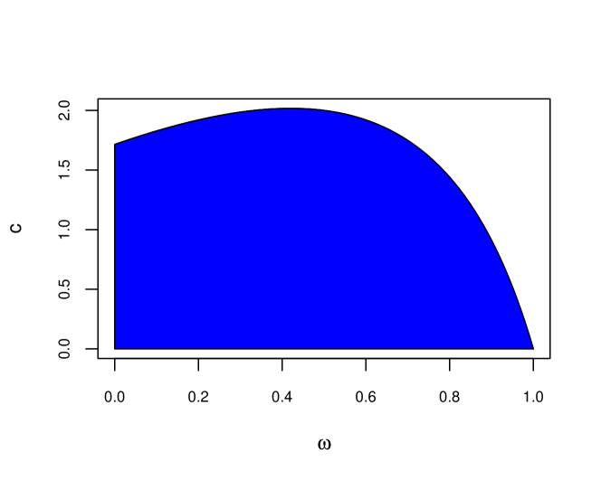
The next Corollary simplifies Theorem 2.1 whenever the convergence of $\mathbb{E}p_{n}$ and $\mathbb{E}g_{n}$ to $p$ and $g$ holds with an appropriate rate. The centering term in the CLT is then $\frac{p+g}{2}$. Denote $\bar{x}_{N}=\frac{1}{N}\sum_{n=1}^{N}x_{n}$.

Corollary 1

If assumption $\mathbf{A_{1-3}}$ hold and if :

$$\frac{1}{\sqrt{N}}\sum_{n=1}^{N}\left(\left|p-\mathbb{E}p_{n}\right|+\left|g-\mathbb{E}g_{n}\right|\right)\rightarrow 0,$$ (2)

then Theorem 2.1 comes down to :

$$\sqrt{N}\left(\bar{x}_{N}-\frac{p+g}{2}\right)\hookrightarrow\mathcal{N}\left(0,\Gamma\right)$$

when $N$tends to infinity.

Remark 1

Condition 2 always holds under stagnation .

The Corollary above shows that the mean computed from the path of the particle converges to $\theta=\left(p+g\right)/2$, losing the information on the location of $p$ and $g$ only. Note that the initial PSO version in 1 (with $c_{1}\neq c_{2}$) would lead to $\theta=\left(c_{1}p+c_{2}g\right)/\left(c_{1}+c_{2}\right)$.

The next Corollary provides finally two kinds of by-products : asymptotic confidence intervals, in $\mathbb{R}$, for the coordinates of $\theta$ and confidence regions for $\theta$ in $\mathbb{R}^{d}$. Let $\alpha\in\left[0,1\right]$, $q_{\alpha}$ be the $1-\alpha$ quantile of the standard Gaussian distribution and $\chi_{1-\alpha}^{\left(d\right)}$ be the $1-\alpha$ quantile of the Chi-square distribution with $d$ degrees of freedom. Set also $\theta=\left(\theta_{1},\ldots,\theta_{d}\right)$ and $\bar{x}_{N}=\left(\bar{x}_{N,1},\ldots,\bar{x}_{N,d}\right)$.

Corollary 2

An asymptotic confidence interval at level $1-\alpha$ for $\theta_{\ell}$ is directly derived from Corollary 1 :

$$\mathcal{I}_{1-\alpha}\left(\theta_{\ell}\right)=\left[\bar{x}_{N,\ell}-s_{\ell}\left(N,\alpha\right);\bar{x}_{N,\ell}+s_{\ell}\left(N,\alpha\right)\right]$$

with $s_{\ell}\left(N,\alpha\right)=\left|p_{\ell}-g_{\ell}\right|\sqrt{\frac{\mathfrak{C}}{N}}q_{1-\frac{\alpha}{2}}$ .
An asymptotic confidence region at level $1-\alpha$ for the vector $\theta=\left(p+g\right)/2$ is :

$$\Lambda_{1-\alpha}\left(\theta\right)=\left\{t\in\mathbb{R}^{d}:N\left\|\Gamma^{-1/2}\left(t-\bar{x}_{N}\right)\right\|^{2}\leq\chi_{1-\alpha}^{\left(d\right)}\right\}$$

$$=\left\{t=\left(t_{1},...,t_{n}\right):\frac{N}{\mathfrak{C}}\sum_{\ell=1}^{d}\left(\frac{t_{\ell}-\bar{x}_{N,\ell}}{p_{\ell}-g_{\ell}}\right)^{2}\leq\chi_{1-\alpha}^{\left(d\right)}\right\}.$$

We note however that the vector $\theta$ may not be of crucial interest for the initial optimization problem conversely to $g$. This point will be discussed in the last section.

Remark 2

Assumption A2 deserves a last but technical remark. First, notice that $\frac{1}{\sqrt{N}}\sum_{n=1}^{N}t_{n}\rightarrow_{\mathbb{P}}0$ does not imply $\lim_{n\rightarrow+\infty}\mathbb{E}\left\|t_{n}\right\|=0$ nor the converse. Take for instance $t_{n}=\left(-1\right)^{n}t_{0}$ with $\mathbb{E}t_{0}\neq 0$ then $\frac{1}{\sqrt{N}}\sum_{n=1}^{N}t_{n}\rightarrow_{\mathbb{P}}0$ whereas $\mathbb{E}\left\|t_{n}\right\|=\mathbb{E}\left\|t_{0}\right\|$. Conversely take $t_{n}=t_{0}/\log\left(n\right)$ $\lim_{n\rightarrow+\infty}\mathbb{E}\left\|t_{n}\right\|=0$ but $\frac{1}{\sqrt{N}}\sum_{n=1}^{N}t_{n}=\frac{t_{0}}{\sqrt{N}}\sum_{n=1}^{N}\log^{-1}\left(n\right)$ cannot converge in probability to 0.

2.2 Second case: non-oscillatory and stagnant ($p=g$)

In this section we study again a single particle and suppose once and for all that $x_{n}\in\mathbb{R}$. We assume throughout this subsection that the particle is under stagnation that is $p_{n}=p$ for $n$ sufficiently large (see assumption $\mathbf{B_{3}}$ below). This assumption is strong but a more general framework leads to theoretical developments out of our scope. Starting from Equation (1), the PSO equation becomes this time:

$$x_{n+1}=\left(1+\omega\right)x_{n}-\omega x_{n-1}+c\left(r_{1,n}+r_{2,n}\right)\left(p-x_{n}\right).$$

Change the centering and consider $x_{n}-p=y_{n}$. The previous equation becomes :

$$y_{n+1}=\left(1+\omega-c+c\varepsilon_{n}\right)y_{n}-\omega y_{n-1},$$ (3)

where $\varepsilon_{n}$ is the sum of two independent random variables with $\mathcal{U}\left[-1/2;1/2\right]$ distribution.

Assuming that for all $n$ $y_{n}\neq 0$, we have then :

$$\frac{y_{n+1}}{y_{n}}=\left(1+\omega-c+c\varepsilon_{n}\right)-\omega\frac{y_{n-1}}{y_{n}}$$ (4)

It is plain that $y_{n+1}/y_{n}$ defines a Markov chain (more precisely : a non-linear auto-regressive process) which will play a crucial role in the proofs and in the forthcoming results. Notice that $\sum_{n=1}^{N}\log\left|\frac{y_{n}}{y_{n-1}}\right|=\log\left|y_{N}\right|-\log\left|y_{0}\right|$.

We are ready to introduce a new set of assumptions. Denote $\pi$ the stationary distribution of $\left(y_{n}/y_{n-1}\right)_{n\in\mathbb{N}}$ and take $\left(Z_{n}\right)_{n\in\mathbb{N}}$ a copy of $\left(y_{n}/y_{n-1}\right)_{n\in\mathbb{N}}$ with $Z_{0}$ a realization of $\pi$. Then define :

$$\mu_{x} =\mathbb{E}_{\pi}\log\left|Z_{0}\right|,$$

$$\sigma_{x}^{2} =\mathrm{Var}_{\pi}\left(\log\left|Z_{0}\right|\right)+2\sum_{k=1}^{+\infty}\mathrm{Cov}_{\pi}\left(\log\left|Z_{0}\right|,\log\left|Z_{k}\right|\right).$$

$\mathbf{B_{1}}:\frac{x_{n}-p}{x_{n-1}-p}$ is a Harris recurrent Markov chain.

$\mathbf{B_{2}}:1+\omega-c<\omega/c<(1+c)/4$.

$\mathbf{B_{3}}:$ For sufficiently large $n$ $g_{n}=p_{n}=p=g$ is constant.

The definition of Harris recurrence needed above is in Meyn and Tweedie (2012), beginning of Chapter 9.

Figure 2: Display of constraint $\mathbf{B}_{2}$ in the plane $\left(c,\omega\right)$.

Theorem 2.2

Let $\omega\in(0,1)$, $c>1$, when $\mathbf{B_{1-3}}$ hold, then:

$$\frac{1}{\sqrt{n}}\left(\log\left|x_{n}-g_{n}\right|-n\mu_{x}\right)\hookrightarrow\mathcal{N}\left(0,\sigma_{x}^{2}\right).$$

Remark 3

The theorem above is not a Central Limit Theorem for $x_{n}$. It is derived thanks to a CLT but it shows that the asymptotic distribution of $\left|x_{n}-g_{n}\right|$ is asymptotically log-normal with approximate parameters $n\mu_{x}$ and $n\sigma_{x}^{2}$.

Remark 4

The mean and variance $\mu_{x}$ and $\sigma_{x}^{2}$ are usually unknown but may be approximated numerically. We refer to the simulation section for more details.

Corollary 3

If $p_{n}=p$ an asymptotic confidence (non convex) region for $g$ at level $1-\alpha$ denoted $\Lambda_{1-\alpha}$ below may be derived from the preceding Theorem:

$$\Lambda_{1-\alpha}\left(g\right) =\Lambda_{1-\alpha}^{+}\cup\Lambda_{1-\alpha}^{-}$$

$$\Lambda_{1-\alpha}^{+} =\left[x_{n}+\exp\left(\mu_{x}+\frac{\sigma_{x}}{\sqrt{n}}q_{\alpha/2}\right),x_{n}+\exp\left(\mu_{x}-\frac{\sigma_{x}}{\sqrt{n}}q_{1-\alpha/2}\right)\right]$$

$$\Lambda_{1-\alpha}^{-} =\left[x_{n}-\exp\left(\mu_{x}+\frac{\sigma_{x}}{\sqrt{n}}q_{1-\alpha/2}\right),x_{n}-\exp\left(\mu_{x}-\frac{\sigma_{x}}{\sqrt{n}}q_{\alpha/2}\right)\right]$$

Remark 5

Under matrix form the equation 3 is purely linear but driven by a random matrix:

$$\left(\begin{array}[c]{c}y_{n+1}\\ y_{n}\end{array}\right) =\mathbf{y}_{n+1}=\left[\begin{array}[c]{cc}1+\omega-c\left(1+\varepsilon_{n}\right)&-\omega\\ 1&0\end{array}\right]\left(\begin{array}[c]{c}y_{n}\\ y_{n-1}\end{array}\right)$$ (11)

$$\mathbf{y}_{n+1} \mathbf{=}\mathbf{S}_{n+1}\mathbf{y}_{n},\quad\mathbf{y}_{n}=\mathbf{S}_{n}\mathbf{S}_{n-1}...\mathbf{S}_{2}\mathbf{y}_{1}=\mathbf{T}_{n}\mathbf{y}_{1},$$

with $\mathbf{T}_{n}=\mathbf{S}_{n}\mathbf{S}_{n-1}...\mathbf{S}_{2}$. It is plain here that a classical Central Limit Theorem cannot hold for the sequence $\left(y_{n}\right)_{n\in\mathbb{N}}$. We turn to asymptotic theory for the product of random matrices. We refer to the historical references: Furstenberg and Kesten (1960) and Berger (1984) who proved Central Limit Theorems for the regularity index of the product of i.i.d random matrices. Later Hennion (1997) generalized their results. But the assumptions of (almost surely) positive entries is common to all these papers. Other authors obtain similar results under different sets of assumptions (see Le Page, 1982, Benoist and Quint, 2016, and references therein), typically revolving around characterization of the semi-group spanned by the distribution of $\mathbf{S}$. These assumptions are uneasy to check here and we carried out to a direct approach with Markov chain fundamental tools.

2.3 The swarm at a fixed step

In this section we change our viewpoint. Instead of considering a single particle and sampling along its trajectory we will take advantage of the whole swarm but at a fixed and common iteration step. Our aim here is to localize the minimum of the cost function based on $\left(x_{n}^{1},\ldots,x_{n}^{S}\right)$. This time the particle index $s$ varies up to $S$ the swarm size, whereas the index $n$ is fixed. In this subsection we assume that $S\uparrow+\infty$ and asymptotic is with respect to $S$. We do not drop $n$ in order to see how the iteration steps influence the results. We still address only the case $x_{n}^{s}\in\mathbb{R}$ even if our results may be straigthforwardly generalized to $x_{n}^{s}\in\mathbb{R}^{d}$. We provide below a Central Limit Theorem suited to the case when the number of particles in the swarm becomes large. In order to clarify the method, we assume that for all particles $x_{n}^{i}$ in the swarm $p_{n}^{i}=g_{n}=p$. In other words, no local minimum stands in the domain $\mathrm{\Omega}$, which implies additional smoothness or convexity assumptions on the cost function $f$. This may be possible by a preliminary screening of the search space. Indeed a first (or several) run(s) of preliminary PSO(s) on the whole domain identifies an area where a single optimum lies. Then a new PSO is launched with initial values close to this optimum and with parameters ensuring that most of the particles will stay in the identified area.

So we are given $\left(x_{n}^{1},...,x_{n}^{S}\right)$ where $S$ is the sample size. Basically, the framework is the same as in the non oscillatory case studied above for a single particle. From (11) we get with $\mathbf{y}_{n}^{i}=x_{n}^{i}-p$ :

$$\mathbf{y}_{n}^{i} = \mathbf{T}_{n}^{i}\mathbf{y}_{1}^{i},$$

$$\mathbf{T}_{n}^{i} = \Pi_{j=2}^{n}\mathbf{S}_{j},\quad\mathbf{S}_{j}=\left[\begin{array}[]{cc}1+\omega-c\left(1+\varepsilon_{j}^{i}\right)&-\omega\\ 1&0\end{array}\right].$$

Assume that the domain $\mathrm{\Omega}$ contains $0$ and that for all $s$ $\left(x_{0}^{i},x_{1}^{i}\right)_{i\leq S}$ are independent, identically distributed and centered then from the decomposition above, for all $n$ and $s$, $\mathbb{E}\mathbf{y}_{n}^{i}=0$ and the $\left(\mathbf{y}_{n}^{i}\right)_{1\leq i\leq S}$ are i.i.d too.

The assumptions we need to derive Theorem 2.3 below are :

$\mathbf{C}_{1}:$ The operational domain $\mathrm{\Omega}$ contains $0$ (and is ideally a symmetric set).

$\mathbf{C}_{2}:$ The couples $\left(x_{0}^{i},x_{1}^{i}\right)_{i\leq S}$ are i.i.d. and centered.

$\mathbf{C}_{3}:$ For all $i$ in $\left\{1,...,S\right\}$ $p_{n}^{i}=g_{n}=p$.

When $S$ is large the following Theorem may be of interest and is a simple consequence of the i.i.d. CLT.

Theorem 2.3

Under assumptions $\mathbf{C}_{1-3}$ a CLT holds when $S$ the number of particles in the swarm tends to $+\infty$ :

$$\frac{1}{\sqrt{S}}\sum_{i=1}^{S}\left(x_{n}^{i}-g_{n}\right)\underset{S\rightarrow+\infty}{\hookrightarrow}\mathcal{N}\left(0,\sigma_{n}^{2}\right),$$

where $\sigma_{n}^{2}=\mathbb{E}\left(x_{n}^{1}-g_{n}\right)^{2}$ is estimated consistently by :

$$\widehat{\sigma}_{n}^{2}=\frac{1}{S}\sum_{i=1}^{S}\left(x_{n}^{i}-g_{n}\right)^{2}.$$

Remark 6

The convergence of $\widehat{\sigma}_{n}^{2}$ to $\sigma_{n}^{2}$ is a straightforward consequence of the weak and strong laws of large numbers.

Denote $\overline{x}^{S}=\left(1/S\right)\sum_{i=1}^{S}x_{n}^{i}$. The Theorem above paves the way towards an asymptotic confidence interval.

Corollary 4

An asymptotic confidence interval at level $1-\alpha$ for $g$ is :

$$\Lambda_{n}\left(g\right)=\left[\overline{x}^{S}-\frac{\widehat{\sigma}_{n}}{\sqrt{S}}q_{1-\alpha/2},\overline{x}^{S}+\frac{\widehat{\sigma}_{n}}{\sqrt{S}}q_{1-\alpha/2}\right].$$

3 Simulation and numerical results

The Himmelblau’s function is chosen as example for our experiments. It is a 2 dimensional function with four local optima in $\left[-10,10\right]^{2}$ defined by : $f(x,y)=\left(x^{2}+y-11\right)^{2}+\left(x+y^{2}-7\right)^{2}$. Figure 3 illustrates the contour of this function.

Figure 3: Contour of the Himmelblau’s function in the space $\left[-6,6\right]^{2}$.

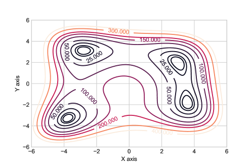
With the Himmelblau’s function, we can observe the two different behaviors of the particles: oscillatory and non-oscillatory. The Himmelblau’s function is positive and has four global minima in: $(3,2)$, $(-2.81,3.13)$, $(-3.77,-3.28)$, $(3.58,-1.84)$ where $f(x,y)=0$. We use a ring topology (for a quick review of the different topologies of PSO see Lane et al. 2008) for the algorithm in order to have both oscillating and non-oscillating particles. The latter converge quickly. The former go on running between two groups of particles converging to two distinct local optima.

3.1 Oscillatory case

We select particles oscillating between $(3.58,-1.84)$ and $(3,2)$, these values could be both their personal best position or their neighborhood best position. In this case, the convergence of the $p_{n}$ and $g_{n}$ to $(3.58,-1.84)$ or $(3,2)$ are satisfying the conditions of Corollary 1. We have to verify the Gaussian asymptotic behavior of $H^{s}_{1}(N)=\sqrt{N}\left(\frac{1}{N}\sum_{n=1}^{N}x^{s}_{n}-\frac{p+g}{2}\right)$ for each $s$ oscillating particle.

We launch PSO with a population of 200 particles and with 2000 iterations, $\omega=0.72984$ and $c=1.496172$. A ring topology was used to ensure the presence of oscillating particles. A particle is said oscillating if between the 500th and the 2000th iteration, Assumptions $\mathbf{A}_{1-3}$ holds.

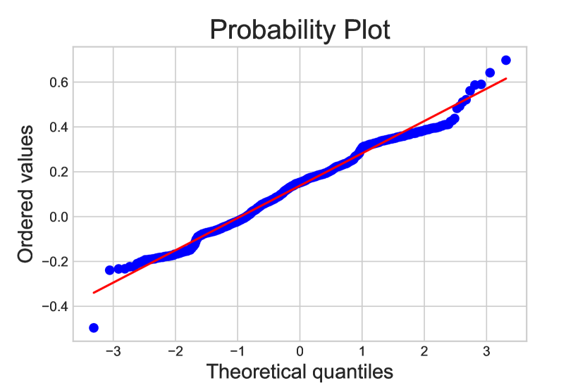
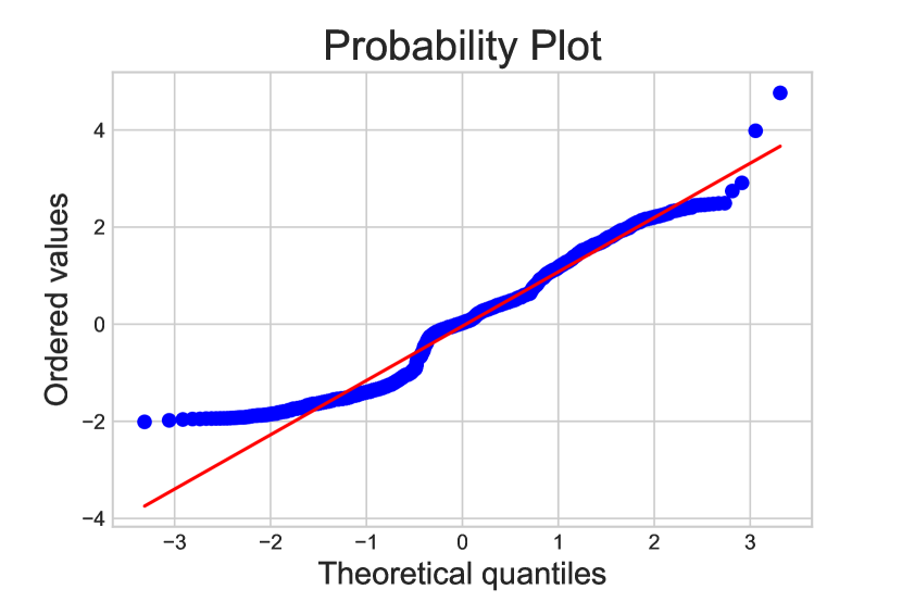
A visual tool to verify the normality of $H^{s}_{1}(N)$ for a particle is a normal probability plot. Figures 5 and 5 displays the normal probability plot of $H^{s}_{1}(N)$ respectively for the $x$ axis and $y$ axis. For each axis, the normality is confirmed: $H^{s}_{1}(N)$ fits well the theoretical quantiles.

Figure 4: Normal probability plot of $H^{s}_{1}(N)$ on the first coordinate.

Figure 5: Normal probability plot of $H^{s}_{1}(N)$ on the second coordinate.

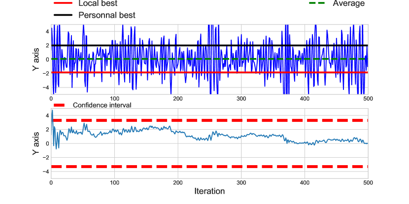
To check the formula of the covariance matrix $\Gamma$, the confidence ellipsoid is also a good indicator (see Figure 6). For a single particle, $H^{s}_{1}(N)$ is not necessarily always inside the confidence ellipsoid and does not respect the percentage of the defined confidence level. Figure 7 shows the trajectory of $x^{s}_{n}$ and $H^{s}_{1}(N)$ on the y axis, $H^{s}_{1}(N)$ remains bounded.

Figure 6: Trajectory of $H^{s}_{1}(N)$ for an oscillating particle in $\left[-10,10\right]^{2}$. The confidence ellipsoid at a level of 85% is displayed in red. Around 99% of the trajectory of $H^{s}_{1}(N)$ is inside the ellipse.

Figure 7: Top track: Trajectory of a oscillating particle on the y axis. The particle is oscillating between 2 and -1.84. Bottom track: corresponding trajectory of $H^{s}_{1}(N)$ on the y axis, the red dot are corresponding to the 95% confidence interval. The trajectory of $H^{s}_{1}(N)$ is well bounded.

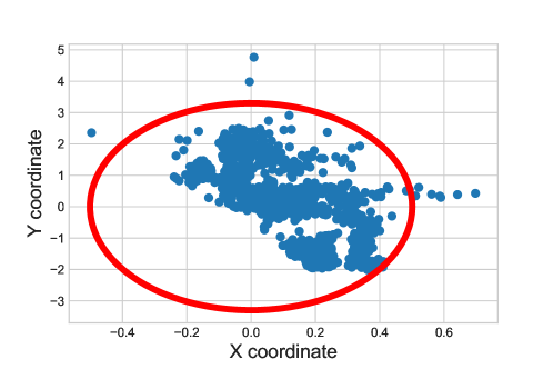
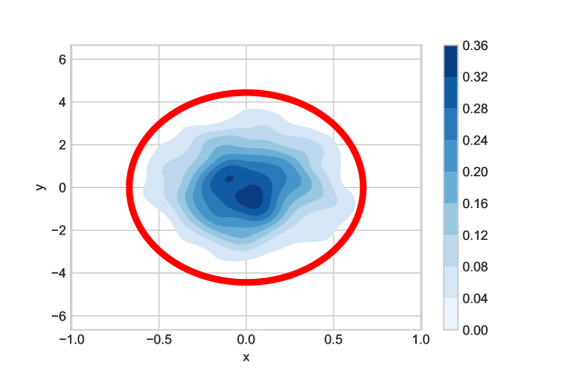
With 200 Monte-Carlo simulations of PSO (200 particles, and 2000 iterations), we select all the particles oscillating between $(3.58,-1.84)$ and $(3,2)$, and for each of them we compute $H^{s}_{1}(2000)$. Figure 8 displayed the density of $H^{s}_{1}(2000)$ using 1150 oscillating particles. Almost 95% of the particles are inside the confidence ellipsoid of level 95% (represented in red).

Figure 8: Density of $H_{1}(2000)$ with 1150 particles issued from Monte-Carlo simulations. The red ellipse is the 95% confidence ellipsoid.

3.2 Non-oscillatory case

We study now the behaviors of non-oscillating particles on the Himmelblau’s function. We launch PSO with a population of 1000 particles and with 2000 iterations, $\omega=0.72984$ and $c=1.496172$. A ring topology was used to ensure the presence of enough particle converging to each local optimum. We select particles converging to $(3,2)$, meaning that $p_{n}=g_{n}=p$ for a sufficiently large $n$. For the weak convergence of the particle, we consider:

$$H^{s}_{2}(N)=\frac{1}{\sqrt{N}}\left(\log\left|x^{s}_{N}-g_{N}\right|-N\mu_{x}\right).$$

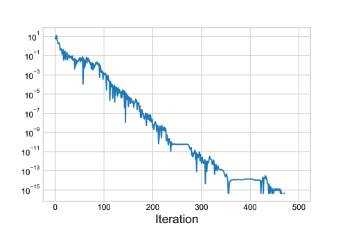
First, it is easy to check the linear dependency of $\log\left|x^{s}_{N}-g_{N}\right|$ with a single display of the trajectory. Figure 9 illustrates this phenomenon for a single particle. We observed numerical issues when we reach the machine precision, but a numerical approximation of $\mu_{x}$ can be performed thanks to a linear regression.

Figure 9: $|x_{n}-g_{n}|$ over 500 iterations in a logarithmic scale. After 300 iterations, we reach the computer precision. We take advantage of the linear behavior of $\log\left(|x_{n}-g_{n}|\right)$ on the 200 first iterations to perform a linear regression estimating $\mu_{x}$.

Using many converging particles, a Monte Carlo approximation of $\mu_{x}$ is done. For the approximation of $\sigma_{x}$, a possibility is:

$$\bar{\sigma}_{x}^{2}=\mathrm{Var}_{\pi}\left(\log\left|X_{0}\right|\right)+2\sum_{k=1}^{T}\mathrm{Cov}_{\pi}\left(\log\left|X_{0}\right|,\log\left|X_{k}\right|\right),$$

where $T=20$. With near 240 converging particles to $(3,2)$, we found that for the first coordinate:

$$\bar{\mu}_{x} =-0.032,$$

$$\bar{\sigma}_{x} =0.156.$$

We verify the asymptotic normality of $H_{2}(N)$ with a normal probability plot using the approximation of $\mu_{x}$. Figure 10 displays the normal probability plot of $H_{2}(N)$ on the first coordinate, the theoretical quantiles are well fitted by $H_{2}(N)$.

Figure 10: Normal probability plot of $H_{2}(N)$ on the first coordinate.

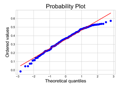
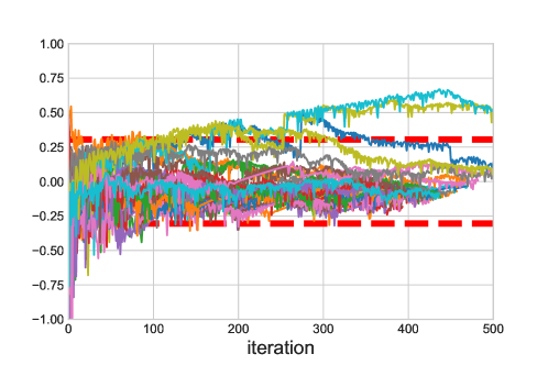
Figure 11 illustrates different trajectories of $H_{2}(N)$ on the first coordinate which are bounded by the 95% confidence interval deduced from $\bar{\sigma}_{x}$.

Figure 11: Trajectories of $H_{2}(N)$ on the first coordinate for five particles. The red dot represents the 95% confidence interval deduced from $\bar{\sigma}_{x}$. Trajectories stop around the 400 iterations (after an heating phase) due to numerical precision.

3.3 Swarm at a fixed step

To check the Theorem 2.3, we study:

$$H^{n}_{3}(S)=\frac{1}{\sqrt{S}\widehat{\sigma}_{n}}\sum_{i=1}^{S}\left(x_{n}^{i}-g_{n}\right).$$

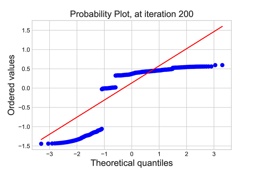
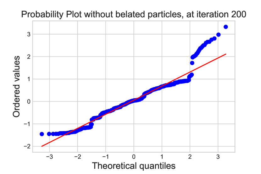
In practice, we encountered some difficulties to verify Theorem 2.3 because of the convergence rate of the particles. Indeed, when $p^{s}_{n}=g^{s}_{n}=p^{s}$, the particle $s$ converges exponentially to $g^{s}_{n}$ but the spread of the rate of convergence is large. As a consequence, at a fixed step of PSO, some particles could be considered as outliers because of a lower rate of convergence. Because of these particles qualified as belated, the asymptotic Gaussian behavior of $H^{n}_{3}(S)$ is not verified. A solution is to filter the particles and remove the belated particles. Figures 13 and 13 illustrate this phenomenon for the Himmelblau’s function in 2D and with near 1500 converging particles to $(3,2)$ over 500 iterations. In Figure 13, we compute without any filtering $H^{n}_{3}(S)$ and we notice that the Gaussian behavior is not verified and some jumps appeared. The presence of these ”jumps” is due to belated particles which have a lower rate of convergence in comparison to the swarm. When we remove these particles with a classical outliers detection algorithm in Figure 13, Theorem 2.3 seems to be verified.

Figure 12: Normal probability plot of $H^{n=200}_{3}(S)$ at the 200th iteration on the first coordinate, using all the particles. We observe a discontinuity of the probability plot due to belated particles.

Figure 13: Normal probability plot of $H^{n=200}_{3}(N)$ at the 200th iteration on the first coordinate, computed without outlying or belated particles.

4 Discussion

Our main theoretical contribution revolves around the three CLTs and the confidence regions derived from sampling either a particle’s path or the whole swarm. Practically the confidence set $\Lambda_{1-\alpha}$ localizes, say $g$, with a high probability. High probability means larger than $1-\alpha$. The simulations carried out in Python language tend to foster the theory.

This work was initiated in order to solve a practical issue in connection with oil industry and petrophysics. Yet in the previous section we confined ourselves to simulated data for several reasons. It appears that our method should be applied on real-data for a clear validation.

A second limitation of our work is the asymptotic set-up. The results are stated for samples large enough. This may not have an obvious meaning for people not familiar with statistics or probability. Practitioners usually claim that the Central Limit Theorem machinery works well for a sample size larger than thirty/forty whenever data are stable, say stationary (path with no jumps…). As a consequence the first iterations of the algorithm should be avoided to ensure a warming. When studying PSO the behavior of $p_{n}$ and $g_{n}$ turns out to be crucial too in order to ensure this stability, hence the validity of the theoretical results. However the control of $p_{n}$ and $g_{n}$ is a difficult matter, which explains our current assumptions on stagnation or “almost stagnation”. However, in order to fix the question of the asymptotic versus non-asymptotic approach a work is on progress. We expect finite-sample concentration inequalities : the non-asymptotic counterparts of CLT.

In the oscillating framework (see Corollary 1) our results involve the parameter denoted $\theta$, the center of the segment $\left[p,g\right]$. Here we miss the target $g$ for instance. We claim that our method may be adapted to tackle this issue. Briefly speaking : running two independent PSOs on the same domain with two distinct pairs $\left(c_{1},c_{2}\right)$ and $\left(c^{\prime}_{1},c^{\prime}_{2}\right)$ will provide, under additional assumptions on the local and global minima of the cost function, two CLTs involving :

$$\theta=\frac{c_{1}g+c_{2}p}{c_{1}+c_{2}}\quad\mathrm{and}\quad\theta^{\prime}=\frac{c^{\prime}_{1}g+c^{\prime}_{2}p}{c^{\prime}_{1}+c^{\prime}_{2}}.$$

A simple matrix inversion then recovers the CLT for e.g. $g$.

5 Derivations of the results

We start with some notations. First we recall that the sup-norm for square matrices of size $d$ defined by:

$$\left\|M\right\|_{\infty}=\sup_{x\neq 0}\frac{\left\|Mx\right\|}{\left\|x\right\|}.$$

The tensor product notation is appropriate when dealing with special kind of matrices for instance covariance matrices. Let $u$ and $v$ be two vectors of $\mathbb{R}^{d}$ then $u\otimes v=uv^{t}$ (where $v^{t}$ is the transpose of vector $v$) stands for the rank one matrix defined for all vector $x$ by $\left(u\otimes v\right)\left(x\right)=\left\langle v,x\right\rangle u$. Besides $\left\|u\otimes v\right\|_{\infty}=\left\|u\right\|\left\|v\right\|$. The Hadamard product between vectors was mentioned earlier. Its matrix version may be defined a similar way. Let $M$ and $S$ be two matrices with same size then $M\odot S$ is the matrix whose $\left(i,j\right)$ cell is $\left(M\odot S\right)_{i,j}=m_{i,j}s_{i,j}$. We recall without proof the following computation rule mixing Hadamard and tensor product. Let $\eta,\varepsilon,u$ and $v$ be four vectors in $\mathbb{R}^{d}$. Then:

$$\left(\eta\odot u\right)\otimes\left(\varepsilon\odot v\right)=\left(\eta\otimes\varepsilon\right)\odot\left(u\otimes v\right),$$ (13)

and the reader must be aware that the Hadamard product on the left-hand side operates between vectors whereas on the right-hand side it operates on matrices.

We will need $\mathcal{F}_{n}^{s}$ the filtration generated by the path of particle number $s$ up to step $n$ : $\left\{x_{0}^{s},...,x_{n}^{s}\right\}$ and $\mathcal{F}_{n}^{\mathcal{S}}$ the filtration generated by the swarm up to step $n$ : $\left\{x_{0}^{s},...,x_{n}^{s}:s=1,...,S\right\}$ .

We will also denote later $g_{n}=\mathbb{E}\left(g_{n}\right)+\xi_{n}$ and $p_{n}=\mathbb{E}\left(p_{n}\right)+\nu_{n}$ the expectation-variance decomposition of $g_{n}$ and $p_{n}$ where $\xi_{n}$ and $\nu_{n}$ are centered random vectors and support all the variability of $g_{n}$ and $p_{n}$ respectively.

5.1 First case: oscillatory

The proof of Theorem 2.1 is developed in the next two subsections. The first subsection below provides some short preliminary results and the proof of the Theorem. The second subsection is devoted to the -somewhat long- derivation of the single Proposition 2. This Proposition 2 is needed within the proof of Theorem 2.1.

5.1.1 Preliminary results and proof of Theorem 2.1

Let us start with some Lemmas who will be invoked later.

Lemma 1

Let $\varepsilon^{\left(i\right)}_{n}$ and $\eta^{\left(j\right)}_{n}$ be any coordinate of the random vectors $\varepsilon_{n}$ and $\eta_{n}$. Clearly, $\varepsilon^{\left(i\right)}_{n}$ and $\eta^{\left(j\right)}_{n}$ are not independent but not correlated and follow the same type of distribution. Besides:

$$\mathbb{E}{\varepsilon^{\left(i\right)}}^{2} =\mathbb{E}{\eta^{\left(j\right)}}^{2}=1/6,\quad\mathbb{E}\varepsilon^{\left(i\right)}\eta^{\left(j\right)}=0,$$

$$\mathbb{E}{\varepsilon^{\left(i\right)}}^{3}\eta^{\left(j\right)} =\mathbb{E}\varepsilon^{\left(i\right)}{\eta^{\left(j\right)}}^{3}=0.$$

The proof is very simple hence omitted.

Lemma 2

When $\mathbf{A}_{1-3}$ hold and when $N$ goes to infinity:

$$\frac{1}{N}\sum_{n=1}^{N}\left\|\frac{\mathbb{E}p_{n}+\mathbb{E}g_{n}}{2}-\mathbb{E}x_{n}\right\|^{2}\rightarrow 0.$$

Proof: Denote $q_{n}=\mathbb{E}x_{n}-\left(\mathbb{E}p_{n}+\mathbb{E}g_{n}\right)/2$. From (14) we get in matrix form:

$$\left(\begin{array}[c]{c}q_{n+1}\\ q_{n}\end{array}\right)=\left[\begin{array}[c]{cc}1+\omega-c&-\omega\\ 1&0\end{array}\right]\left(\begin{array}[c]{c}q_{n}\\ q_{n-1}\end{array}\right)+\left(\begin{array}[c]{c}K_{n}\\ 0\end{array}\right)$$

where:

$$K_{n+1}=\left(1+\omega\right)\mathbb{E}\left(p_{n}\mathbb{+}g_{n}\right)-\omega\mathbb{E}\left(p_{n-1}\mathbb{+}g_{n-1}\right)-\mathbb{E}\left(p_{n+1}\mathbb{+}g_{n+1}\right).$$

The above equation may be rewritten $\mathbf{q}_{n+1}=\mathbf{Mq}_{n}+\mathbf{K}_{n+1}$ with obvious but shorter notations. Notice that in $K_{n}$ each $\mathbb{E}\left(p_{k}\mathbb{+}g_{k}\right)$, $k\in\{n-1,n,n+1\}$ may be replaced by $\mathbb{E}\left(p_{k}\mathbb{+}g_{k}\right)-\left(p+g\right)$. Consequently, we know that $K_{n}$ tends to $0$. Also notice that $\|\mathbf{M}\|_{\infty}<1$ because $\omega<1$.

Then we derive:

$$\mathbf{q}_{n}\mathbf{=}\sum_{p=2}^{n}\mathbf{M}^{n-p}\mathbf{K}_{p}.$$

It suffices to notice now that if $\mathbf{q}_{n}$ decays to $0,$ so does $\left\|\mathbf{q}_{n}\right\|$ and Lemma 2 will be derived by a simple application of Cesaro’s famous Lemma. Let us prove now that $\mathbf{q}_{n}\downarrow 0$.

Take $\varepsilon>0$ denote $K_{\infty}=\max\left(\left\|\mathbf{K}_{p}\right\|\right)$ and $C_{M}=\left[1-\left\|\mathbf{M}\right\|_{\infty}\right]^{-1}.$ First pick $N^{\ast}$ such that $\sup_{p\geq N^{\ast}+1}\left\|\mathbf{K}_{p}\right\|<\varepsilon/\left(2C_{M}\right)$

$$\left\|\mathbf{q}_{n}\right\| \leq\sum_{p=2}^{N^{\ast}}\left\|\mathbf{M}\right\|_{\infty}^{n-p}\left\|\mathbf{K}_{p}\right\|+\sum_{p=N^{\ast}+1}^{n}\left\|\mathbf{M}\right\|_{\infty}^{n-p}\left\|\mathbf{K}_{p}\right\|$$

$$\leq\left\|\mathbf{M}\right\|_{\infty}^{n-N^{\ast}}\sum_{p=2}^{N^{\ast}}\left\|\mathbf{M}\right\|_{\infty}^{n-p}\left\|\mathbf{K}_{p}\right\|+\max_{p\geq N^{\ast}+1}\left\|\mathbf{K}_{p}\right\|\sum_{p=N^{\ast}+1}^{n}\left\|\mathbf{M}\right\|_{\infty}^{n-p}$$

$$\leq C_{M}\left[K_{\infty}\left\|\mathbf{M}\right\|_{\infty}^{n-N^{\ast}}+\sup_{p\geq N^{\ast}+1}\left\|\mathbf{K}_{p}\right\|.\right]$$

Then let $N^{{\dagger}}$ be such that $\left\|\mathbf{M}\right\|_{\infty}^{N^{{\dagger}}}<\varepsilon/\left(2C_{M}K_{\infty}\right)$. It can be seen from the equations above that for $n>N^{{\dagger}}+N^{\ast}$, $\left\|\mathbf{\ q}_{n}\right\|<\varepsilon$.

The following Proposition is crucial:

Proposition 1

Let $S_{N}=\sum_{n=1}^{N}z_{n}$ then:

$$S_{N}=\sum_{n=1}^{N}\left[\frac{\eta_{n}}{2}\odot\left(p_{n}-g_{n}\right)-\varepsilon_{n}\odot z_{n}\right]+\sum_{n=1}^{N}\tilde{r}_{n}+\frac{1}{c}\left(z_{1}-\omega z_{0}+\omega z_{N}-z_{N+1}\right).$$

Under assumptions $\mathbf{A}_{2}$

$$\frac{1}{\sqrt{N}}\sum_{n=1}^{N}\tilde{r}_{n}\rightarrow_{\mathbb{P}}0.$$

Besides when $\mathbf{A}_{1}$ holds (the $x_{n}^{\prime}$s are almost surely bounded) then $S_{N}/\sqrt{N}$ converges weakly if and only if:

$$\frac{1}{\sqrt{N}}\sum_{n=1}^{N}\left[\frac{\eta_{n}}{2}\odot\left(p_{n}-g_{n}\right)-\varepsilon_{n}\odot z_{n}\right]$$

converges weakly too.

Proof of Proposition 1: The first equation is obtained by summing from $n=1$ to $N$ both sides of Equation (15). Then we are going to prove that $\frac{1}{\sqrt{N}}\sum_{n=1}^{N}\tilde{r}_{n}\rightarrow_{\mathbb{P}}0$ by Markov inequality which will be enough to get the rest of the Proposition. We start from $\tilde{r}_{n}=\varepsilon_{n}\left(\frac{\mathbb{E}p_{n}+\mathbb{E}g_{n}}{2}-\mathbb{E}x_{n}\right)+\frac{1+\varepsilon_{n}}{2}\left(p_{n}-\mathbb{E}p_{n}+g_{n}-\mathbb{E}g_{n}\right)$. By the first part of assumption $\mathbf{A}_{2}$

$$\frac{1}{\sqrt{N}}\sum_{n=1}^{N}\left(p_{n}-\mathbb{E}p_{n}\right)\rightarrow_{\mathbb{P}}0\quad\frac{1}{\sqrt{N}}\sum_{n=1}^{N}\left(g_{n}-\mathbb{E}g_{n}\right)\rightarrow_{\mathbb{P}}0.$$

We turn to:

$$\mathbb{E}\left\|\sum_{n=1}^{N}\varepsilon_{n}\left(\frac{\mathbb{E}p_{n}+\mathbb{E}g_{n}}{2}-\mathbb{E}x_{n}\right)\right\|^{2}=\mathbb{E}\varepsilon_{1}^{2}\sum_{n=1}^{N}\left\|\frac{\mathbb{E}p_{n}+\mathbb{E}g_{n}}{2}-\mathbb{E}x_{n}\right\|^{2}$$

because $\varepsilon_{n}$ is an i.i.d. centered sequence. The proposition now follows from Lemma 2. This completes the proof of the Proposition.

Proposition 1 shows that the limiting distribution of $S_{N}$ is completely determined by the limiting distribution of $\sum_{n=1}^{N}\left[\frac{\eta_{n}}{2}\odot\left(p_{n}-g_{n}\right)-\varepsilon_{n}\odot z_{n}\right]$. If a Central Limit Theorem holds for the previous series, then the limiting distribution will depend on the covariance matrix of $\frac{\eta_{n}}{2}\odot\left(p_{n}-g_{n}\right)-\varepsilon_{n}\odot z_{n}$. The latter will be decomposed in several terms.

Proof of Theorem 2.1:

As a preliminary step, let us rewrite (1) on a single line :

$$x_{n+1}=\left(1+\omega\right)x_{n}-\omega x_{n-1}+c\left(r_{1,n}+r_{2,n}\right)\odot\left(\frac{p_{n}+g_{n}}{2}-x_{n}\right)+c\left(r_{1,n}-r_{2,n}\right)\odot\frac{p_{n}-g_{n}}{2}.$$

Taking expectation:

$$\mathbb{E}x_{n+1}=\left(1+\omega\right)\mathbb{E}x_{n}-\omega\mathbb{E}x_{n-1}+c\left(\frac{\mathbb{E}p_{n}+\mathbb{E}g_{n}}{2}-\mathbb{E}x_{n}\right).$$ (14)

By subtracting, denoting the centered process $z_{n}=x_{n}-\mathbb{E}x_{n}$ and $e$ the vector of $\mathbb{R}^{d}$ defined by $e=\left(1,1,...,1\right)$ the PSO equation becomes :

$$z_{n+1}=\left(1+\omega-c\right)z_{n}-\omega z_{n-1}-c\varepsilon_{n}\odot z_{n}+c\tilde{r}_{n}+\frac{c}{2}\eta_{n}\odot\left(p_{n}-g_{n}\right),$$ (15)

with

$$\varepsilon_{n} =r_{1,n}+r_{2,n}-e\quad\eta_{n}=r_{1,n}-r_{2,n},$$

$$\tilde{r}_{n} =\varepsilon_{n}\odot\left(\frac{\mathbb{E}p_{n}+\mathbb{E}g_{n}}{2}-\mathbb{E}x_{n}\right)+\frac{e+\varepsilon_{n}}{2}\odot\left(p_{n}-\mathbb{E}p_{n}+g_{n}-\mathbb{E}g_{n}\right).$$

Equation (15) will be a starting point especially for studying single particle trajectories.

We turn to the Theorem. From:

$$\frac{1}{N}\sum_{n=1}^{N}x_{n}-\frac{1}{N}\sum_{n=1}^{N}\frac{\mathbb{E}p_{n}+\mathbb{E}g_{n}}{2}=\frac{1}{N}\sum_{n=1}^{N}z_{n}+\frac{1}{N}\sum_{n=1}^{N}\left(\mathbb{E}x_{n}-\frac{\mathbb{E}p_{n}+\mathbb{E}g_{n}}{2}\right),$$

we see from the proof of Lemma 2 that $\left(1/\sqrt{N}\right)\sum_{n=1}^{N}\left[\mathbb{E}x_{n}-\left(\mathbb{E}p_{n}+\mathbb{E}g_{n}\right)/2\right]\rightarrow 0$ as $N$ tends to infinity. Following Proposition 1, the Theorem 2.1 comes down to proving:

$$\frac{1}{\sqrt{N}}\sum_{n=1}^{N}\left[\frac{\eta_{n}}{2}\odot\left(p_{n}-g_{n}\right)-\varepsilon_{n}\odot z_{n}\right]\hookrightarrow\mathcal{N}\left(0,\Gamma\right).$$

We can first remark that $u_{n}=\frac{\eta_{n}}{2}\odot\left(p_{n}-g_{n}\right)-\varepsilon_{n}\odot z_{n}$ is a vector-valued martingale difference sequence with respect to the filtration $\mathcal{F}_{n}^{s}=\mathcal{F}_{n}$. We confine ourselves to proving a Levy-Lindeberg version of the CLT for the series of $u_{n}$ in two steps (Theorem 2.1.9 p. 46 and its corollary 2.1.10 in Duflo, 1997): first ensuring convergence of the conditional covariance structure of $\left(1/\sqrt{N}\right)\sum_{n=1}^{N}u_{n}$, then checking the Lyapunov condition holds (hence the Lindeberg’s uniform integrability that ensures uniform tightness of the sequence).

First step: The conditional covariance sequence of $u_{n}$ is the sequence of matrices defined by $\frac{1}{N}\sum_{n=1}^{N}\mathbb{E}\left(u_{n}\otimes u_{n}|\mathcal{F}_{n}\right)$. We show in this first step that this sequence converges in probability to $\Gamma$. We start with elementary calculations:

$$\frac{1}{N}\sum_{n=1}^{N}\mathbb{E}\left(u_{n}\otimes u_{n}|\mathcal{F}_{n}\right) =\frac{1}{N}\sum_{n=1}^{N}\mathbb{E}\left(\frac{\eta_{n}}{2}\odot\left(p_{n}-g_{n}\right)\otimes\frac{\eta_{n}}{2}\odot\left(p_{n}-g_{n}\right)|\mathcal{F}_{n}\right)$$

$$+\frac{1}{N}\sum_{n=1}^{N}\mathbb{E}\left(\left(\varepsilon_{n}\odot z_{n}\right)\otimes\left(\varepsilon_{n}\odot z_{n}\right)|\mathcal{F}_{n}\right)$$

$$-\frac{1}{2N}\sum_{n=1}^{N}\mathbb{E}\left(\left[\eta_{n}\odot\left(p_{n}-g_{n}\right)\right]\otimes\left[\varepsilon_{n}\odot z_{n}\right]|\mathcal{F}_{n}\right)$$

$$-\frac{1}{2N}\sum_{n=1}^{N}\mathbb{E}\left(\left[\varepsilon_{n}\odot z_{n}\right]\otimes\left[\eta_{n}\odot\left(p_{n}-g_{n}\right)\right]|\mathcal{F}_{n}\right)$$

$$=\frac{\mathbb{E}\varepsilon_{1}^{2}}{N}\mathbf{I}\odot\left\{\sum_{n=1}^{N}\frac{1}{4}\left[\left(p_{n}-g_{n}\right)\otimes\left(p_{n}-g_{n}\right)\right]+z_{n}\otimes z_{n}\right\}$$

$$=\frac{1}{6}\mathbf{I}\odot\left[\frac{1}{4}\Gamma_{N,p,g}+\Gamma_{N,z}\right],$$

where we used Lemma 1 and denoted $\Gamma_{N,p,g}=\frac{1}{N}\sum_{n=1}^{N}\left[\left(p_{n}-g_{n}\right)\otimes\left(p_{n}-g_{n}\right)\right]$ and :

$$\Gamma_{N,z}=\frac{1}{N}\sum_{n=1}^{N}z_{n}\otimes z_{n},$$

By Proposition 2 stated and proved in the next subsection, $\Gamma_{N,z}-\frac{\mathfrak{H}}{N}\Gamma_{N,p,g}$ tends in probability to zero. Hence whenever the limit in the r.h.s below exists:

$$\lim_{N\rightarrow+\infty}\frac{1}{N}\sum_{n=1}^{N}\mathbb{E}\left(u_{n}\otimes u_{n}|\mathcal{F}_{n}\right)=\left(\frac{1}{24}+\frac{\mathfrak{H}}{6}\right)\lim_{N\rightarrow+\infty}\mathbf{I}\odot\Gamma_{N,p,g}.$$

Under assumption $\mathbf{A}_{1-2}$ $\lim_{N\rightarrow+\infty}\Gamma_{N,p,g}-\overline{\Gamma}_{N,p,g}=0$ in matrix norm, where

$$\overline{\Gamma}_{N,p,g}=\frac{1}{N}\sum_{n=1}^{N}\mathbb{E}\left[\left(p_{n}-g_{n}\right)\otimes\mathbb{E}\left(p_{n}-g_{n}\right)\right].$$

To prove this it suffices to write:

$$\Gamma_{N,p,g}-\overline{\Gamma}_{N,p,g}=\frac{1}{N}\sum_{n=1}^{N}\left(\nu_{n}-\xi_{n}\right)\otimes\left(p_{n}-g_{n}\right)+\frac{1}{N}\sum_{n=1}^{N}\mathbb{E}\left(p_{n}-g_{n}\right)\otimes\left(\nu_{n}-\xi_{n}\right),$$

and apply the bounds derived from the proof of Proposition 2, for instance:

$$\frac{1}{N}\left\|\sum_{n=1}^{N}\left(\nu_{n}-\xi_{n}\right)\otimes\left(p_{n}-g_{n}\right)\right\|_{\infty} \leq\frac{1}{N}\sum_{n=1}^{N}\left\|\left(\nu_{n}-\xi_{n}\right)\otimes\left(p_{n}-g_{n}\right)\right\|_{\infty}$$

$$\leq\frac{1}{N}\sum_{n=1}^{N}\left\|\nu_{n}-\xi_{n}\right\|\left\|p_{n}-g_{n}\right\|$$

$$\leq\sup_{n}\left\|p_{n}-g_{n}\right\|\frac{1}{N}\sum_{n=1}^{N}\left(\left\|\nu_{n}\right\|+\left\|\xi_{n}\right\|\right)\rightarrow_{\mathbb{P}}0.$$

Finally, the convergence of $\overline{\Gamma}_{N,p,g}$ to $\Gamma$ is a consequence of the adaptation of Cesaro’s Lemma for tensor products.

Second step: A Lyapunov condition holds almost trivially here. Namely we are going to prove that:

$$\frac{1}{N^{2}}\sum_{n=1}^{N}\mathbb{E}\left\|u_{n}\right\|^{4}\rightarrow_{N\rightarrow+\infty}0.$$

Simple calculations provide:

$$\left\|u_{n}\right\|^{2} \leq 2\left\|\frac{\eta_{n}}{2}\odot\left(p_{n}-g_{n}\right)\right\|^{2}+2\left\|\varepsilon_{n}\odot z_{n}\right\|^{2}$$

$$\leq\frac{1}{2}\sup_{n,i}\{\left(p_{n,i}-g_{n,i}\right)^{2}\}\left\|\eta_{n}\right\|^{2}+2\sup_{n,i}\{z_{n,i}^{2}\}\left\|\varepsilon_{n}\right\|^{2}$$

$$\leq 2\left|\mathrm{\Omega}\right|_{\infty}^{2}\left[\left\|\eta_{n}\right\|^{2}+\left\|\varepsilon_{n}\right\|^{2}\right],$$

with $\left|\mathrm{\Omega}\right|_{\infty}=\sup_{s\in\mathrm{\Omega}}\left|s\right|$ hence

$$\mathbb{E}\left\|u_{n}\right\|^{4}\leq C\left|\mathrm{\Omega}\right|_{\infty}^{4},$$

for some constant $C$ then $\left(1/N^{2}\right)\sum_{n\leq N}\mathbb{E}\left\|u_{n}\right\|^{4}$ tends to zero when $N$ tends to infinity. This completes the proof of Theorem 2.1.

5.1.2 Proof of Proposition 2

We are ready to state and prove this important intermediate result.

Proposition 2

Under assumption $A_{3}$ denote:

$$\mathfrak{H}=\frac{c^{2}}{24}\left(2c\left(\frac{1-\omega}{1+\omega}\right)\left(1+\omega-\frac{c}{2}\right)-\frac{c^{2}}{6}\right)^{-1},$$

then when $N$ tends to $+\infty$

$$\Gamma_{N,z}-\frac{\mathfrak{H}}{N}\sum_{n=1}^{N}\mathrm{diag}\left(\delta_{n}^{\odot 2}\right)\rightarrow_{\mathbb{P}}0,$$

with $\delta_{n}=p_{n}-g_{n}$.

The proof of the Proposition will immediately follow from this Lemma.

Lemma 3

Let $E_{n}$ be a sequence of i.i.d centered random matrices with finite moment of order 4, let $u_{n}$ and $v_{n}$ two sequence of random vectors almost surely bounded and such that $\left(u_{n},v_{n}\right)$ is for all $n$ independent from $E_{n}$ then for the $\left\|\cdot\right\|_{\infty}$ norm:

$$\frac{1}{N}\sum_{n=1}^{N}E_{n}\odot\left(u_{n}\otimes v_{n}\right)\rightarrow_{\mathbb{P}}0.$$

The proof of the above Lemma is a straightforward application of Cauchy-Schwartz inequality.

Proof of the Proposition 2: We take advantage of Equation (15) and note that

$$\left(\varepsilon_{n}\odot z_{n}\right)\otimes\left(\varepsilon_{n}\odot z_{n}\right) =\left(\varepsilon_{n}\otimes\varepsilon_{n}\right)\odot\left(z_{n}\otimes z_{n}\right)$$

$$=\left[\left(\varepsilon_{n}\otimes\varepsilon_{n}\right)-\sigma_{\varepsilon}^{2}\mathbf{I}\right]\odot\left(z_{n}\otimes z_{n}\right)+\sigma_{\varepsilon}^{2}\mathbf{I}\odot\left(z_{n}\otimes z_{n}\right),$$

where $\sigma_{\varepsilon}^{2}=1/6$ by Lemma 1 and $\mathbf{I}$ stands for identity matrix. After some tedious calculations we obtain:

$$z_{n+1}\otimes z_{n+1} =\left(1+\omega-c\right)^{2}\left(z_{n}\otimes z_{n}\right)+\omega^{2}z_{n-1}\otimes z_{n-1}$$ (16)

$$+c^{2}\sigma_{\varepsilon}^{2}\left[\mathbf{I}\odot\left(z_{n}\otimes z_{n}\right)\right]+\frac{c^{2}}{4}\left[\eta_{n}\odot\left(p_{n}-g_{n}\right)\right]\otimes\left[\eta_{n}\odot\left(p_{n}-g_{n}\right)\right]$$

$$-\omega\left(1+\omega-c\right)\left[z_{n}\otimes z_{n-1}+z_{n-1}\otimes z_{n}\right]+\mathcal{C}_{n}.$$

For the sake of completeness, we list now all the eleven terms contained in $\mathcal{C}_{n}$. In order to simplify notations let $\left[\left[u:v\right]\right]=u\otimes v+v\otimes u$. Notice for further use:

$$\left\|\left[\left[u:v\right]\right]\right\|_{\infty}\leq 2\left\|u\right\|\left\|v\right\|.$$

Then:

$$\mathcal{C}_{n} =c\left(1+\omega-c\right)\left\{\left[\left[z_{n}:\tilde{r}_{n}\right]\right]-\left[\left[z_{n}:\varepsilon_{n}\odot z_{n}\right]\right]+\frac{1}{2}\left[\left[z_{n}:\eta_{n}\odot\left(p_{n}-g_{n}\right)\right]\right]\right\}$$ (17)

$$+\omega c\left\{\left[\left[z_{n-1}:\varepsilon_{n}\odot z_{n}\right]\right]-\left[\left[z_{n-1}:\tilde{r}_{n}\right]\right]-\frac{1}{2}\left[\left[z_{n-1}:\eta_{n}\odot\left(p_{n}-g_{n}\right)\right]\right]\right\}$$

$$-c^{2}\left\{\left[\left[c\varepsilon_{n}\odot z_{n}:\tilde{r}_{n}\right]\right]+\frac{1}{2}\left[\left[\varepsilon_{n}\odot z_{n}:\eta_{n}\odot\left(p_{n}-g_{n}\right)\right]\right]-\frac{1}{2}\left[\left[\tilde{r}_{n}:\eta_{n}\odot\left(p_{n}-g_{n}\right)\right]\right]\right\}$$

$$+c^{2}\tilde{r}_{n}\otimes\tilde{r}_{n}+c^{2}\left[\left(\varepsilon_{n}\otimes\varepsilon_{n}\right)-\sigma_{\varepsilon}^{2}\mathbf{I}\right]\odot\left(z_{n}\otimes z_{n}\right).$$

From 16 we sum over all indices $n$ in $\left\{1,...,N\right\}$ we get:

$$\left(1-\left(1+\omega-c\right)^{2}-\omega^{2}\right)\sum_{n=1}^{N}z_{n}\otimes z_{n} =c^{2}\sigma_{\varepsilon}^{2}\sum_{n=1}^{N}\left[\mathbf{I}\odot\left(z_{n}\otimes z_{n}\right)\right]$$

$$+\frac{c^{2}}{4}\sum_{n=1}^{N}\left[\eta_{n}\odot\left(p_{n}-g_{n}\right)\right]\otimes\left[\eta_{n}\odot\left(p_{n}-g_{n}\right)\right]$$

$$-\omega\left(1+\omega-c\right)\sum_{n=1}^{N}\left[z_{n}\otimes z_{n-1}+z_{n-1}\otimes z_{n}\right]$$

$$+\sum_{n=1}^{N}\mathcal{C}_{n}+z_{1}\otimes z_{1}-z_{N+1}\otimes z_{N+1}$$

$$+\omega^{2}\left(z_{0}\otimes z_{0}-z_{N}\otimes z_{N}\right).$$

Now we need to go slightly further in the computations and to find a recurrent equation for $z_{n}\otimes z_{n-1}$. Let us start again from (15):

$$z_{n+1}\otimes z_{n} =\left(1+\omega-c\right)z_{n}\otimes z_{n}-\omega z_{n-1}\otimes z_{n}-c\left(\varepsilon_{n}\odot z_{n}\right)\otimes z_{n}+c\tilde{r}_{n}\otimes z_{n}$$

$$+\frac{c}{2}\left[\eta_{n}\odot\left(p_{n}-g_{n}\right)\right]\otimes z_{n},$$

$$z_{n}\otimes z_{n+1} =\left(1+\omega-c\right)z_{n}\otimes z_{n}-\omega z_{n}\otimes z_{n-1}-cz_{n}\otimes\left(\varepsilon_{n}\odot z_{n}\right)+cz_{n}\otimes\tilde{r}_{n}$$

$$+\frac{c}{2}z_{n}\otimes\left[\eta_{n}\odot\left(p_{n}-g_{n}\right)\right].$$

Summing over all indices $n$ in $\left\{1,...,N\right\}$ above we come to

$$\left(1+\omega\right)\sum_{n=1}^{N}\left[z_{n}\otimes z_{n-1}+z_{n-1}\otimes z_{n}\right]$$

$$=z_{1}\otimes z_{0}+z_{0}\otimes z_{1}-z_{N}\otimes z_{N+1}-z_{N+1}\otimes z_{N}+2\left(1+\omega-c\right)\sum_{n=1}^{N}\left[z_{n}\otimes z_{n}\right]$$

$$+c\sum_{n=1}^{N}\left\{\left[\left[\tilde{r}_{n}:z_{n}\right]\right]-\left[[\left(\varepsilon_{n}\odot z_{n}\right):z_{n}\right]]+\frac{1}{2}\left[\left[\eta_{n}\odot\left(p_{n}-g_{n}\right):z_{n}\right]\right]\right\}.$$

Plugging the last equation in line (16) we get finally:

$$\left(1-\left(1+\omega-c\right)^{2}-\omega^{2}\right)\sum_{n=1}^{N}z_{n}\otimes z_{n}$$

$$=c^{2}\sigma_{\varepsilon}^{2}\sum_{n=1}^{N}\left[\mathbf{I}\odot\left(z_{n}\otimes z_{n}\right)\right]+\frac{c^{2}}{4}\sum_{n=1}^{N}\left[\eta_{n}\odot\left(p_{n}-g_{n}\right)\right]\otimes\left[\eta_{n}\odot\left(p_{n}-g_{n}\right)\right]$$

$$-2\omega\frac{\left(1+\omega-c\right)^{2}}{1+\omega}\sum_{n=1}^{N}\left[z_{n}\otimes z_{n}\right]+\omega c\frac{\left(1+\omega-c\right)}{1+\omega}\sum_{n=1}^{N}\left[[\left(\varepsilon_{n}\odot z_{n}\right):z_{n}\right]]$$

$$-\omega c\frac{\left(1+\omega-c\right)}{1+\omega}\sum_{n=1}^{N}\left[\left[\tilde{r}_{n}:z_{n}\right]\right]-\omega c\frac{\left(1+\omega-c\right)}{\left(1+\omega\right)}\sum_{n=1}^{N}\frac{1}{2}\left[\left[\eta_{n}\odot\left(p_{n}-g_{n}\right):z_{n}\right]\right]+\sum_{n=1}^{N}\mathcal{C}_{n}.$$

Denoting $\kappa=\left(1-\left(1+\omega-c\right)^{2}-\omega^{2}+2\omega\frac{\left(1+\omega-c\right)^{2}}{1+\omega}\right)=2c\left(\frac{1-\omega}{1+\omega}\right)\left(1+\omega-\frac{c}{2}\right)$:

$$\kappa\sum_{n=1}^{N}z_{n}\otimes z_{n}=\frac{c^{2}}{6}\sum_{n=1}^{N}\left[\mathbf{I}\odot\left(z_{n}\otimes z_{n}\right)\right]+\frac{c^{2}}{4}\sum_{n=1}^{N}\left[\eta_{n}\odot\left(p_{n}-g_{n}\right)\right]\otimes\left[\eta_{n}\odot\left(p_{n}-g_{n}\right)\right]+\mathfrak{R}_{N},$$

with

$$\mathfrak{R}_{N} =-\omega\frac{\left(1+\omega-c\right)}{1+\omega}\left(\left[\left[z_{1}:z_{0}\right]\right]-\left[\left[z_{N}:z_{N+1}\right]\right]\right)+z_{1}\otimes z_{1}-z_{N+1}\otimes z_{N+1}$$ (18)

$$+\omega^{2}\left(z_{0}\otimes z_{0}-z_{N}\otimes z_{N}\right)+\sum_{n=1}^{N}\mathcal{C}_{n}$$

$$+\omega c\frac{\left(1+\omega-c\right)}{1+\omega}\sum_{n=1}^{N}\left\{\left[[\left(\varepsilon_{n}\odot z_{n}\right):z_{n}\right]]-\left[\left[\tilde{r}_{n}:z_{n}\right]\right]-\frac{1}{2}\left[\left[\eta_{n}\odot\left(p_{n}-g_{n}\right):z_{n}\right]\right]\right\}.$$

It is proved in Lemma 4 that $\mathfrak{R}_{N}/N\rightarrow_{\mathbb{P}}0$. First, let us unravel the matrix:

$$\mathbf{T}_{N}=\frac{\kappa}{N}\sum_{n=1}^{N}z_{n}\otimes z_{n}-\frac{c^{2}}{6}\frac{1}{N}\sum_{n=1}^{N}\left[\mathbf{I}\odot\left(z_{n}\otimes z_{n}\right)\right].$$

Denote $\left[\mathbf{T}_{N}\right]_{ij}$ the $\left(i,j\right)$ cell of matrix $\mathbf{T}_{n}.$ It is simple to see that:

$$\left[\mathbf{T}_{N}\right]_{ii}=\left(\kappa-\frac{c^{2}}{6}\right)\left[\frac{1}{N}\sum_{n=1}^{N}\left(z_{n}\otimes z_{n}\right)\right]_{ii},\quad\left[\mathbf{T}_{N}\right]_{ij}=\kappa\left[\frac{1}{N}\sum_{n=1}^{N}z_{n}\otimes z_{n}\right]_{i,j}$$ (19)

for $i\neq j$. Now denote:

$$\Lambda_{N} =\frac{1}{N}\sum_{n=1}^{N}\left[\eta_{n}\odot\left(p_{n}-g_{n}\right)\right]\otimes\left[\eta_{n}\odot\left(p_{n}-g_{n}\right)\right]$$

$$=\frac{1}{N}\sum_{n=1}^{N}\left(\eta_{n}\otimes\eta_{n}\right)\odot\left[\left(p_{n}-g_{n}\right)\otimes\left(p_{n}-g_{n}\right)\right].$$

Taking conditional expectation w.r.t $\mathcal{F}_{n}$ we get -all non diagonal term vanish:

$$\mathbb{E}\left(\Lambda_{N}|\mathcal{F}_{n}\right) =\frac{1}{N}\sum_{n=1}^{N}\left[\mathbb{E}\left(\eta_{n}\otimes\eta_{n}\right)\right]\odot\left[\left(p_{n}-g_{n}\right)\otimes\left(p_{n}-g_{n}\right)\right]$$

$$=\frac{\mathbb{E}\eta_{1}^{2}}{N}\sum_{n=1}^{N}\mathbf{I}\odot\left[\left(p_{n}-g_{n}\right)\otimes\left(p_{n}-g_{n}\right)\right],$$

with $\mathbf{I}$ the identity matrix. Noting that the difference:

$$\Lambda_{N}-\mathbb{E}\left(\Lambda_{N}|\mathcal{F}_{n}\right)=\frac{1}{N}\sum_{n=1}^{N}\left[\left(\eta_{n}\otimes\eta_{n}\right)-\left(\mathbb{E}\eta_{1}^{2}\right)\mathbf{I}\right]\odot\left[\left(p_{n}-g_{n}\right)\otimes\left(p_{n}-g_{n}\right)\right]$$

vanishes when $N$ tends to infinity by applying Lemma 3 we get with Landau notation in probability:

$$\mathbf{T}_{N}=\frac{c^{2}}{24N}\sum_{n=1}^{N}\mathbf{I}\odot\left[\left(p_{n}-g_{n}\right)\otimes\left(p_{n}-g_{n}\right)\right]+o_{P}\left(\frac{1}{N}\right).$$

From (19) we obtain simultaneously that $\left[\mathbf{T}_{N}\right]_{ij}\rightarrow_{\mathbb{P}}0$ for $i\neq j$ and

$$\left[\mathbf{T}_{N}\right]_{ii}-\frac{c^{2}}{24\left(\kappa-\frac{c^{2}}{6}\right)}\frac{1}{N}\sum_{n=1}^{N}\mathbf{I}\odot\left[\left(p_{n}-g_{n}\right)\otimes\left(p_{n}-g_{n}\right)\right]\rightarrow_{\mathbb{P}}0$$

which is precisely the statement of Proposition 2.

Lemma 4

$\mathfrak{R}_{N}/N\rightarrow_{\mathbb{P}}0$ in matrix norm.

Proof: Let us start from (18). First by assumption $\mathbf{A}_{1}$:

$$\frac{1}{N}\left(\left[\left[z_{1}:z_{0}\right]\right]-\left[\left[z_{N}:z_{N+1}\right]\right]\right)+z_{1}\otimes z_{1}-z_{N+1}\otimes z_{N+1}+\omega^{2}\left(z_{0}\otimes z_{0}-z_{N}\otimes z_{N}\right)\rightarrow_{\mathbb{P}}0.$$

It must be also noticed that:

$$\omega c\frac{\left(1+\omega-c\right)}{1+\omega}\sum_{n=1}^{N}\left\{\left[[\left(\varepsilon_{n}\odot z_{n}\right):z_{n}\right]]-\left[\left[\tilde{r}_{n}:z_{n}\right]\right]-\frac{1}{2}\left[\left[\eta_{n}\odot\left(p_{n}-g_{n}\right):z_{n}\right]\right]\right\}$$

involves three terms between double brackets that already appear in $\mathcal{C}_{n}$, up to constants. Proving that each term of $\left(1/N\right)\sum_{n=1}^{N}\mathcal{C}_{n}$ tends in probability to $0$ will be sufficient to complete the proof of the Lemma.

Our aim is to perform successive applications of Lemma 3. For the sake of completeness we remind now the eleven terms contained in $\mathcal{C}_{n}$ and mentioned earlier.

$$\mathcal{C}_{n} =c\left(1+\omega-c\right)\left\{\left[\left[z_{n}:\tilde{r}_{n}\right]\right]-\left[\left[z_{n}:\varepsilon_{n}\odot z_{n}\right]\right]+\frac{1}{2}\left[\left[z_{n}:\eta_{n}\odot\left(p_{n}-g_{n}\right)\right]\right]\right\}$$

$$+\omega c\left\{\left[\left[z_{n-1}:\varepsilon_{n}\odot z_{n}\right]\right]-\left[\left[z_{n-1}:\tilde{r}_{n}\right]\right]-\frac{1}{2}\left[\left[z_{n-1}:\eta_{n}\odot\left(p_{n}-g_{n}\right)\right]\right]\right\}$$

$$-c^{2}\left\{\left[\left[c\varepsilon_{n}\odot z_{n}:\tilde{r}_{n}\right]\right]+\frac{1}{2}\left[\left[\varepsilon_{n}\odot z_{n}:\eta_{n}\odot\left(p_{n}-g_{n}\right)\right]\right]-\frac{1}{2}\left[\left[\tilde{r}_{n}:\eta_{n}\odot\left(p_{n}-g_{n}\right)\right]\right]\right\}$$

$$+c^{2}\tilde{r}_{n}\otimes\tilde{r}_{n}+c^{2}\left[\left(\varepsilon_{n}\otimes\varepsilon_{n}\right)-\sigma_{\varepsilon}^{2}\mathbf{I}\right]\odot\left(z_{n}\otimes z_{n}\right).$$

In the list above terms numbered 2, 3, 4, 6, 11 vanish by applying successively (13) and Lemma 3. Take for instance term 1, get rid of the constants and focus on the first tensor product in the double bracket namely:

$$z_{n}\otimes\left(\varepsilon_{n}\odot z_{n}\right)=\left(e\odot z_{n}\right)\otimes\left(\varepsilon_{n}\odot z_{n}\right)=\left(e\otimes\varepsilon_{n}\right)\odot\left(z_{n}\otimes z_{n}\right).$$

Recall that $e$ is the vector with all components valued at $1.$ Then we can apply Lemma 3 which shows that $\left(1/N\right)\sum_{n=1}^{N}\left(e\otimes\varepsilon_{n}\right)\odot\left(z_{n}\otimes z_{n}\right)$ vanishes in probability. It is not hard to see that terms 3, 4, 6 and 11 may be treated the same way.

Term number 8 namely depends on both $\varepsilon_{n}$ and $\eta_{n}$. An application of (13) leads to considering, up to a constant and commutation to:

$$\left(\eta_{n}\otimes\varepsilon_{n}\right)\odot\left(z_{n}\otimes\left(p_{n}-g_{n}\right)\right).$$

The reader can check that the matrix $E_{n}=\left(\eta_{n}\otimes\varepsilon_{n}\right)$ is stochastically independent from $z_{n}\otimes\left(p_{n}-g_{n}\right)$, that the sequence of matrices $E_{n}$ are independent and centered. Lemma 3 applies here.

The terms numbered 1, 5, 7, 9, 10 depend on $\tilde{r}_{n}.$ Now consider

$$\tilde{r}_{n}=\varepsilon_{n}\odot\left(\frac{\mathbb{E}p_{n}+\mathbb{E}g_{n}}{2}-\mathbb{E}x_{n}\right)+\frac{e+\varepsilon_{n}}{2}\odot\left(\xi_{n}+\nu_{n}\right)=r_{n1}+r_{n2},$$

and the five terms containing them in $\mathcal{C}_{n}$. We split $\tilde{r}_{n}$ and deal separately with $r_{n1}$ and $r_{n2}$ to derive the needed bounds in probability.

First, let us focus on $r_{n1}=\varepsilon_{n}\odot\left(\frac{\mathbb{E}p_{n}+\mathbb{E}g_{n}}{2}-\mathbb{E}x_{n}\right)$ only. Once again Lemma 3 may be invoked for the specific halves of terms 1, 5 and 9 by using the same methods as above. The half part of terms 7 and 10 of (17) containing $\varepsilon_{n}$ may be bounded the following way (denote $\beta_{n}=\frac{\mathbb{E}p_{n}+\mathbb{E}g_{n}}{2}-\mathbb{E}x_{n}$):

$$\left\|\left[\left[\varepsilon_{n}\odot z_{n}:\varepsilon_{n}\odot\beta_{n}\right]\right]\right\|_{\infty} \leq 2\left\|z_{n}\right\|\left\|\beta_{n}\right\|,$$

$$\left\|\left(\varepsilon_{n}\odot\beta_{n}\right)\otimes\left(\varepsilon_{n}\odot\beta_{n}\right)\right\|_{\infty} \leq 2\left\|\beta_{n}\right\|^{2}.$$

Lemma 2 ensures that both right hand sides above tend to zero (since $\sup_{n}\left\|z_{n}\right\|$ is almost surely bounded) and Cesaro’s Lemma terminates this part.

We should now inspect the terms numbered 1, 5, 7, 9, 10 in (17) with respect to $r_{n2}=\frac{e+\varepsilon_{n}}{2}\odot\left(\xi_{n}+\nu_{n}\right)$. Terms 7 and 9 may be controlled by Lemma 2 and Lemma 3 respectively. Let us deal with term 1:

$$\left\|\sum_{n=1}^{N}\left[\left[z_{n}:r_{n2}\right]\right]\right\|_{\infty} \leq 2\sum_{n=1}^{N}\left\|z_{n}\right\|\left\|r_{n2}\right\|$$

$$\leq 2\left(\sup_{n}\left\|z_{n}\right\|\right)\sum_{n=1}^{N}\left\|r_{n2}\right\|$$

$$\leq 2\sup_{n}\left\|z_{n}\right\|\sum_{n=1}^{N}\left[\left\|\nu_{n}\right\|+\left\|\xi_{n}\right\|\right].$$

Take for instance $\sum_{n=1}^{N}\left\|\nu_{n}\right\|$. Applying Markov inequality:

$$\mathbb{P}\left(\frac{1}{N}\sum_{n=1}^{N}\left\|\nu_{n}\right\|>\varepsilon\right)\leq\frac{1}{N}\sum_{n=1}^{N}\mathbb{E}\left\|\nu_{n}\right\|,$$

then Assumption $\mathbf{A}_{2}$ together with Cesaro’s Lemma again ensure that $\frac{1}{N}\sum_{n=1}^{N}\left\|\nu_{n}\right\|\rightarrow_{\mathbb{P}}0$ as well as $\frac{1}{N}\sum_{n=1}^{N}\left\|\xi_{n}\right\|$ hence $\frac{1}{N}\left\|\sum_{n=1}^{N}\left[\left[z_{n}:r_{n2}\right]\right]\right\|_{\infty}$. Term 5 vanishes in probability with the same technique at hand. Now term 10 gives:

$$\left\|\frac{1}{N}\sum_{n=1}^{N}r_{2n}\otimes r_{2n}\right\|_{\infty}\leq\frac{1}{N}\sum_{n=1}^{N}\left\|r_{2n}\otimes r_{2n}\right\|_{\infty}=\frac{1}{N}\sum_{n=1}^{N}\left\|r_{2n}\right\|^{2}$$

which also tends to zero in probability under $\mathbf{A}_{1-2}$. By the way we mention that the cross-product $\left[\left[r_{1n}:r_{2n}\right]\right]$ in term 10 vanishes due to Lemma 2. Our task is almost done. Let us deal now with the remaining terms of $\mathfrak{R}_{N}$. Both:

$$\frac{1}{N}\sum_{n=1}^{N}\left[\left(\varepsilon_{n}\odot z_{n}\right)\otimes z_{n}+z_{n}\otimes\left(\varepsilon_{n}\odot z_{n}\right)\right],$$

$$\frac{1}{N}\sum_{n=1}^{N}\left[\eta_{n}\odot\left(p_{n}-g_{n}\right)\right]\otimes z_{n}+z_{n}\otimes\left[\eta_{n}\odot\left(p_{n}-g_{n}\right)\right]$$

tends to $0$ in probability by Lemma 3 and (13). At last, the remaining $\left[\left[\tilde{r}_{n}:z_{n}\right]\right]$ is basically the same as term 1 in (17) and may be addressed the same way. This terminates the proof of the Lemma.

5.2 Second case: non-oscillatory and stagnant

We start from 4 and set $X_{n}=y_{n}/y_{n-1}$. Then we get :

$$X_{n+1}=1+\omega-c-\frac{\omega}{X_{n}}+c\varepsilon_{n},$$

where $\varepsilon_{n}=r_{1,n}+r_{2,n}-1$ has a “witch hat” distribution (convolution of two uniform distributions) with support $\left[-1,+1\right]$. We focus now on the above homogeneous Markov chain $X_{n}$ and we aim at proving that a CLT holds for $h\left(X_{n}\right)=\log\left|X_{n}\right|$ namely that for some $\mu$ and $\sigma^{2}$ :

$$\sqrt{N}\left[\frac{1}{N}\sum_{n=1}^{N}\log\left|X_{n}\right|-\mu\right]\hookrightarrow\mathcal{N}\left(0,\sigma^{2}\right),$$

which will yield:

$$\sqrt{N}\left[\frac{1}{N}\log\left|y_{N}\right|-\mu\right]\hookrightarrow\mathcal{N}\left(0,\sigma^{2}\right).$$

We aim at applying Theorem 1 p.302 in Jones (2004). We need to check two points: existence of a small set $\mathcal{C}$ and of a function $g$ with a drift condition (see Meyn and Tweedie, 2012).

Denote $P\left(t,x\right)$ the transition kernel of $X_{n}$. It is plain that $P\left(t,x\right)$ coincides with the density of the uniform distribution on the set $\mathcal{E}_{x}=\left[1+\omega-2c-\frac{\omega}{x},1+\omega-\frac{\omega}{x}\right]$. The Theorem 2.2 is a consequence of the two Lemmas below coupled with the above-mentioned Theorem 1 p.302 in Jones (2004).

Lemma 5

Take $M_{\tau}=\omega/\left(c-\tau\right)$ with any $0<\tau<c$ then the set $\mathcal{C}=\left(-\infty,-M_{\tau}\right]\cup\left[M_{\tau},+\infty\right)$ is a small set for the transition kernel of $X_{n}$.

Proof:

We have to show that for all $x\in\mathcal{C}$ and Borel set $A$ in $\mathbb{\ R}$:

$$P\left(A,x\right)\geq\varepsilon Q\left(A\right),$$

where $\varepsilon>0$ and $Q$ is a probability distribution. The main problem here comes from the compact support of $P\left(t,x\right)$. Take $x$ such that $\left|x\right|\geq M$ then:

$$1+\omega-c-\frac{\omega}{M}+c\varepsilon_{n}\leq 1+\omega-c-\frac{\omega}{x}+c\varepsilon_{n}\leq 1+\omega-c+\frac{\omega}{M}+c\varepsilon_{n},$$

where $\varepsilon_{n}$ has compact support $\left[-1,+1\right]$. It is simple to see that with $M=M_{\tau}=\omega/\left(c-\tau\right)$ the above bound becomes:

$$1+\omega-2c+\tau+c\varepsilon_{n}\leq 1+\omega-c-\frac{\omega}{x}+c\varepsilon_{n}\leq 1+\omega+\tau+c\varepsilon_{n}.$$

The intersection of the supports of $1+\omega-2c+\tau+c\varepsilon_{n}$ and $1+\omega-2c+\tau+c\varepsilon_{n}$ is the set $\left[1+\omega-c-\tau,1+\omega-c+\tau\right]$ whatever the value of $x$ in $\mathcal{C}$. The probability measure $Q$ mentioned above may be chosen with support $\left[1+\omega-c-\tau,1+\omega-c+\tau\right]$.

Now we turn to the drift condition. Our task consists in constructing a function
$g:\mathbb{R}\rightarrow\left[1,+\infty\right[$ such that for all $x$:

$$\int_{\mathbb{R}}g\left(t\right)P\left(t,x\right)dt\leq\rho_{1}g\left(x\right)+\rho_{2}1_{x\in\mathcal{C}},$$ (20)

where $0<\rho_{1}<1$ and $\rho_{2}\geq 0.$ Besides, in order to get a CLT on $\log\left|X_{n}\right|$ we must further ensure that for all $x$:

$$\left[\log\left|x\right|\right]^{2}\leq g\left(x\right).$$ (21)

Note however that, if (20) holds for $g$ but (21) fails, then both conditions will hold for updated function $g^{\ast}=\eta g$ with constant $\eta>1$ and $\rho_{2}^{\prime}=\eta\rho_{2}$ such that (21) holds.

Lemma 6

Take for $g$ the even function defined by $g\left(x\right)=C_{1}/\sqrt{\left|x\right|}$ for $\left|x\right|\leq M_{\tau}$ and $g\left(x\right)=C_{2}\left(\log\left|x\right|\right)^{2}$ for $\left|x\right|>M_{\tau}$. Assume that:

$$\mathbf{B}_{2}:1+\omega-c<\omega/c<\left(1+c\right)/4.$$

Then it is always possible to choose three constants $\tau,$ $C_{1}$ and $C_{2}$ such that (20) holds for a specific choice of $\rho_{1}$ and $\rho_{2}$.

Proof:

The proof of the Lemma just consists in an explicit construction of the above-mentioned $\tau$, $C_{1}$, and $C_{2}$. This construction is detailed for the sake of completeness.

At this point and in order to simplify the computations below we will assume that the distribution of $\varepsilon_{n}$ is uniform on $\left[-1,+1\right]$ instead of the convolution of two $\mathcal{U}_{\left[-1/2,1/2\right]}$ distributions.

Set $\lambda=1+\omega-c$, assume that $\lambda>0$ (the case $\lambda<0$ follows the same lines) and notice that:

$$\int_{\mathbb{R}}g\left(t\right)P\left(t,x\right)dt=\frac{1}{2c}\int_{\mathbb{\lambda-}\left(\omega/x\right)-c}^{\mathbb{\lambda-}\left(\omega/x\right)+c}g\left(s\right)ds=\frac{1}{2c}\int_{\left(\omega/x\right)-\lambda-c}^{\left(\omega/x\right)-\lambda+c}g\left(s\right)ds,$$

the last inequality stemming from parity of $g$. We should consider two cases $x>0$ and $x\leq 0$.

The proof takes 2 parts ($x>0$ and $x<0$ respectively). Both are given again for completeness and because the problem is not symmetric. Each part is split in three steps: the two first steps deal with $x\notin\mathcal{C}$, the third with $x\in\mathcal{C}=\left(-\infty,-M_{\tau}\right]\cup\left[M_{\tau},+\infty\right)$.

Part 1: $x>0$

First step: We split $\left[0,M_{\tau}\right]$ in two subsets, $\left[0,M_{\tau}\right]=\left[0,A_{\tau}\right]\cup\left[A_{\tau},M_{\tau}\right]$ with

$$A_{\tau}=\omega/\left(M_{\tau}+1+\omega\right)$$

is chosen such that $0\leq x\leq A_{\tau}$ implies the following inequality on the lower bound of the integral: $\left(\omega/x\right)-\lambda-c>M_{\tau}$. Clearly $A_{\tau}\leq M_{\tau}$ because $\lambda>0>-\tau-M_{\tau}$. Then:

$$\frac{1}{2c}\int_{\left(\omega/x\right)-\lambda-c}^{\left(\omega/x\right)-\lambda+c}g\left(s\right)ds=\frac{C_{2}}{2c}\int_{\left(\omega/x\right)-\lambda-c}^{\left(\omega/x\right)-\lambda+c}\log^{2}\left|s\right|ds\leq C_{2}\log^{2}\left|\left(\omega/x\right)-\lambda+c\right|.$$

Let:

$$\sup_{0\leq x\leq\omega/\left(c+M_{\tau}\right)}\sqrt{\left|x\right|}\left(\log\left|\left(\omega/x\right)-\lambda+c\right|\right)^{2}=K_{1}\left(\omega,c,\tau\right)<+\infty.$$

The strictly positive $K_{1}\left(\omega,c,\tau\right)$ exists because $\sqrt{x}\log^{2}\left|\left(\omega/x\right)-\lambda+c\right|$ is bounded on $\left[0,A_{\tau}\right]$. The first condition reads:

$$\frac{1}{2c}\int_{\left(\omega/x\right)-\lambda-c}^{\left(\omega/x\right)-\lambda+c}g\left(s\right)ds\leq\rho_{1}C_{1}/\sqrt{\left|x\right|},\qquad 0\leq x\leq A_{\tau}$$

whenever

$$C_{2}K_{1}\left(\omega,c,\tau\right)\leq\rho_{1}C_{1}$$ (22)

and $\rho_{1}$ will be fixed after the second step.

Second step: Now we turn to $A_{\tau}\leq x\leq M_{\tau}$. We still have $g\left(x\right)=C_{1}/\sqrt{\left|x\right|}$ but we need to focus on the bounds of the integral.

This time the lower bound of the integral $\left(\omega/x\right)-\lambda-c\in\left[-\lambda-\tau,M_{\tau}\right]$ and the upper bound $\left(\omega/x\right)-\lambda+c\in\left[2c-\lambda-\tau,2c+M_{\tau}\right]$. We are going to require that $\left(\omega/x\right)-\lambda-c\geq-M_{\tau}$ it suffices to take $\lambda+\tau\leq M_{\tau}$ and this comes down to the following set of constraint on $\tau$: $\left\{\tau\geq c-\omega\right\}\cup\left\{\tau\leq c-1\right\}.$ We keep the second and assume once and for all that:

$$\tau\leq c-1.$$ (23)

Then for $x\in\left[A_{\tau},M_{\tau}\right]$,

$$\frac{1}{2c}\int_{\left(\omega/x\right)-\lambda-c}^{\left(\omega/x\right)-\lambda+c}g\left(s\right)ds =\frac{1}{2c}\int_{\left(\omega/x\right)-\lambda-c}^{M_{\tau}}g\left(s\right)ds+\frac{1}{2c}\int_{M_{\tau}}^{\left(\omega/x\right)-\lambda+c}g\left(s\right)ds$$ (24)

$$\equiv\mathcal{I}_{1}+\mathcal{I}_{2}.$$

We want to make sure that the upper bound $\left(\omega/x\right)-\lambda+c$ is larger than $M_{\tau}$. This will hold if $\left(\omega/M_{\tau}\right)-\lambda+c\geq M_{\tau}$ hence if $2c-\tau-\lambda\geq M_{\tau}.$ We imposed previously that $\lambda+\tau\leq M_{\tau}$. So:

$$\tau<c-\frac{\omega}{c}\Rightarrow M_{\tau}<c\Rightarrow 2c-\tau-\lambda\geq M_{\tau}$$

but the constraint $\tau<c-\omega/c$ is weaker than (23) consequently (24) holds.

Focus on the first term $\mathcal{I}_{1}$ in (24) and consider:

$$\mathcal{I}_{1}=\frac{1}{2c}\int_{\left(\omega/x\right)-\lambda-c}^{M_{\tau}}g\left(s\right)ds=\frac{1}{2c}\int_{\left(\omega/x\right)-\lambda-c}^{M_{\tau}}\frac{C_{1}}{\sqrt{\left|s\right|}}ds.$$

Consider the (only) two situations on the sign of $\left(\omega/x\right)-\lambda-c=\left(\omega/x\right)-\left(1+\omega\right)$.
If $x<\omega/\left(1+\omega\right)$ then $\left(\omega/x\right)-\left(1+\omega\right)>0$ and $\mathcal{I}_{1}\leq\frac{C_{1}}{c}\sqrt{M_{\tau}}$ Notice by the way and for further purpose that:

$$\sup_{x\in\left[A_{\tau},\omega/\left(1+\omega\right)\right]}\sqrt{\left|x\right|}\mathcal{I}_{1}\leq\frac{C_{1}}{c}\sqrt{\frac{\omega}{1+\omega}M_{\tau}}.$$

If $x\geq\omega/\left(1+\omega\right)$ then $\left(\omega/x\right)-\left(1+\omega\right)\leq 0$ and:

$$\mathcal{I}_{1} =\frac{1}{2c}\int_{\left(\omega/x\right)-\lambda-c}^{M_{\tau}}g\left(s\right)ds=\frac{1}{2c}\int_{\left(\omega/x\right)-\left(1+\omega\right)}^{0}\frac{C_{1}}{\sqrt{\left|s\right|}}ds+\frac{1}{2c}\int_{0}^{M_{\tau}}\frac{C_{1}}{\sqrt{\left|s\right|}}ds$$

$$=\frac{C_{1}}{c}\left[\sqrt{\left|\left(\omega/x\right)-\left(1+\omega\right)\right|}+\sqrt{M_{\tau}}\right].$$

Again:

$$\sqrt{\left|x\right|}\mathcal{I}_{1}\leq\frac{C_{1}}{c}\left[\sqrt{\left|x\left(1+\omega\right)-\omega\right|}+\sqrt{xM_{\tau}}\right].$$

From the bounds above we see that:

$$\sup_{x\in\left[A_{\tau},M_{\tau}\right]}\sqrt{\left|x\right|}\mathcal{I}_{1}\leq\frac{C_{1}}{c}\left[\sqrt{\left|M_{\tau}\left(1+\omega\right)-\omega\right|}+M_{\tau}\right].$$

The reader will soon understand why we need to make sure that the right had side in equation above is strictly under $C_{1}$. It is not hard to see that the function $\tau\longmapsto\sqrt{\left|M_{\tau}\left(1+\omega\right)-\omega\right|}+M_{\tau}$ is increasing and continuous on $\left[0,c-1\right]$. If we prove that for some $\delta\in\left]0,1\right[$:

$$\frac{1}{c}\left[\sqrt{\left|M_{0}\left(1+\omega\right)-\omega\right|}+M_{0}\right]=1-3\delta<1,$$

then the existence of some $\tau^{+}>0$ such that:

$$\frac{1}{c}\left[\sqrt{\left|M_{\tau^{+}}\left(1+\omega\right)-\omega\right|}+M_{\tau^{+}}\right]=1-2\delta<1$$ (25)

will be granted. But $\frac{1}{c}\left[\sqrt{\left|M_{0}\left(1+\omega\right)-\omega\right|}+M_{0}\right]=\frac{1}{c}\left[\sqrt{\frac{\omega}{c}\lambda}+\frac{\omega}{c}\right].$
If we assume that $\lambda<\omega/c<\left(1+c\right)/4$ (assumption $\mathbf{B}_{2}$) then since $c>1$:

$$\frac{1}{c}\left[\sqrt{\frac{\omega}{c}\lambda}+\frac{\omega}{c}\right]<\frac{1}{2}\left(1+\frac{1}{c}\right)<1.$$

We turn to $\mathcal{I}_{2}$ in (24):

$$\mathcal{I}_{2}=\frac{1}{2c}\int_{M_{\tau}}^{\left(\omega/x\right)-\lambda+c}g\left(s\right)ds=\frac{C_{2}}{2c}\int_{M_{\tau}}^{\left(\omega/x\right)-\lambda+c}\left(\log s\right)^{2}ds\leq\frac{C_{2}}{\sqrt{\left|x\right|}}K_{2}\left(\omega,c,\tau^{+}\right),$$

where:

$$K_{2}\left(\omega,c,\tau^{+}\right)=\sup_{x\in\left[A_{\tau},M_{\tau}\right]}\frac{\sqrt{\left|x\right|}}{2c}\int_{M_{\tau}}^{\left(\omega/x\right)-\lambda+c}\left(\log s\right)^{2}ds.$$

Set finally $\rho_{1}^{+}=1-\delta<1$.

From (24) we get:

$$\frac{1}{2c}\int_{\left(\omega/x\right)-\lambda-c}^{\left(\omega/x\right)-\lambda+c}g\left(s\right)ds \leq\frac{C_{1}}{\sqrt{\left|x\right|}}.\left(1-2\delta\right)+\frac{C_{2}}{\sqrt{\left|x\right|}}K_{2}\left(\omega,c,\tau^{+}\right)$$

$$\leq\rho_{1}^{+}\frac{C_{1}}{\sqrt{\left|x\right|}},$$

whenever holds the new condition:

$$C_{2}K_{2}\left(\omega,c,\tau\right)\leq C_{1}\delta.$$ (26)

Finally comparing (22) and (26), we see that both conditions cannot be incompatible. Accurate choices of the couple $\left(C_{1}^{+},C_{2}^{+}\right)$ are given by the summary bound:

$$C_{2}^{+}\leq C_{1}^{+}\min\left(\frac{\delta}{K_{2}},\frac{1-\delta}{K_{1}}\right).$$ (27)

It is now basic to see that the quadruple $\left(C_{1}^{+},C_{2}^{+},\tau^{+},\rho_{1}^{+}\right)$ yields the drift condition (20) for $x\notin\mathcal{C}$.

Third step: The remaining step is to check the inequality for some $\rho_{2}$:

$$\int_{\mathbb{R}}g\left(t\right)P\left(t,x\right)dt\leq\rho_{1}^{+}g\left(x\right)+\rho_{2},$$

for any $x$ in $\mathcal{C}$ -that is any $\left|x\right|>M_{\tau}$ (rather $x>M_{\tau}$ here as explained above since $x>0$). We see that:

$$0\leq\frac{\omega}{x}\leq\frac{\omega}{M_{\tau}},$$

and:

$$\frac{1}{2c}\int_{\left(\omega/x\right)-\lambda-c}^{\left(\omega/x\right)-\lambda+c}g\left(s\right)ds\leq\frac{1}{2c}\int_{-\lambda-c}^{2c-\tau-\lambda}g\left(s\right)ds\leq\frac{1}{2c}\int_{-\left(1+\omega\right)}^{3c-\left(1+\omega\right)}g\left(s\right)ds.$$

The values of the constants $C_{1}$ and $C_{2}$ were fixed above. Then denote:

$$\rho_{2}^{+}=\frac{1}{2c}\int_{-\left(1+\omega\right)}^{3c-\left(1+\omega\right)}g\left(s\right)ds>0,$$

then clearly for any $x$ in $\mathcal{C}$:

$$\int_{\mathbb{R}}g\left(t\right)P\left(t,x\right)dt\leq\rho_{2}^{+},$$

so that (20) holds.

Part 2 ($x\leq 0$)

We go on with $x<0$ and $\lambda>0,$ set $y=-x\geq 0,$

$$\int_{\mathbb{R}}g\left(t\right)P\left(t,x\right)dt=\frac{1}{2c}\int_{\mathbb{\lambda-}\left(\omega/x\right)-c}^{\mathbb{\lambda-}\left(\omega/x\right)+c}g\left(s\right)ds=\frac{1}{2c}\int_{\left(\omega/y\right)+\lambda-c}^{\left(\omega/y\right)+\lambda+c}g\left(s\right)ds.$$

Since $g$ is even and in view of the proposed $\mathcal{C}$ we just have to prove exactly the following drift condition with $x>0$:

$$\frac{1}{2c}\int_{\left(\omega/x\right)+\lambda-c}^{\left(\omega/x\right)+\lambda+c}g\left(s\right)ds\leq\rho_{1}g\left(x\right)+\rho_{2}1_{x\in\mathcal{C}}.$$

First step: Take $x\notin\mathcal{C}$. We split $\left[0,M_{\tau}\right]$ in two subsets, $\left[0,M_{\tau}\right]=\left[0,B_{\tau}\right]\cup\left[B_{\tau},M_{\tau}\right]$ with $B_{\tau}=\omega/\left(M_{\tau}-\lambda+c\right)$ is chosen such that $0\leq x\leq B_{\tau}$ implies the following inequality on the lower bound of the integral: $\left(\omega/x\right)+\lambda-c>M_{\tau}$. Clearly $B_{\tau}\leq M_{\tau}$ for all $\tau$. Then:

$$\frac{1}{2c}\int_{\left(\omega/x\right)+\lambda-c}^{\left(\omega/x\right)+\lambda+c}g\left(s\right)ds=\frac{C_{2}}{2c}\int_{\left(\omega/x\right)+\lambda-c}^{\left(\omega/x\right)+\lambda+c}\log^{2}\left|s\right|ds\leq C_{2}\log^{2}\left|\left(\omega/x\right)+\lambda+c\right|.$$

Let:

$$\sup_{0\leq x\leq B_{\tau}}\sqrt{\left|x\right|}\log^{2}\left|\left(\omega/x\right)+\lambda+c\right|=K_{1}\left(\omega,c,\tau\right)<+\infty.$$

The strictly positive $K_{1}\left(\omega,c,\tau\right)$ exists because $\sqrt{\left|x\right|}\log^{2}\left|\left(\omega/x\right)+\lambda+c\right|$ is bounded on $\left[0,B_{\tau}\right]$. The initial condition reads:

$$\frac{1}{2c}\int_{\left(\omega/x\right)+\lambda-c}^{\left(\omega/x\right)+\lambda+c}g\left(s\right)ds\leq\rho_{1}C_{1}/\sqrt{\left|x\right|},\qquad 0\leq x\leq B_{\tau}$$

whenever $C_{2}K_{1}\left(\omega,c,\tau\right)\leq\rho_{1}C_{1}$ and $\rho_{1}$ will be fixed later.

Second step: Now we turn to $B_{\tau}\leq x\leq M_{\tau}$. We still have $g\left(x\right)=C_{1}/\sqrt{\left|x\right|}$ but we need to focus on the bounds of the integral.

This time the lower bound of the integral $\left(\omega/x\right)+\lambda-c\in\left[\lambda-\tau,M_{\tau}\right]$ and the upper bound $\left(\omega/x\right)+\lambda+c\in\left[\lambda+2c-\tau,M_{\tau}+2c\right]$. If we assume that $\tau\leq\lambda$ then $\left(\omega/x\right)+\lambda-c\geq 0\geq-M_{\tau}.$ Besides in order that $\lambda+2c-\tau\geq M_{\tau}$ we just have need that $2c\geq M_{\tau}$ or $\tau\leq c-\omega/\left(2c\right).$ As a consequence the assumption:

$$\tau\leq\min\left(\lambda,c-\frac{\omega}{2c}\right)$$ (28)

allows to write for $x\in\left[B_{\tau},M_{\tau}\right]$,

$$\frac{1}{2c}\int_{\left(\omega/x\right)+\lambda-c}^{\left(\omega/x\right)+\lambda+c}g\left(s\right)ds =\frac{1}{2c}\int_{\left(\omega/x\right)+\lambda-c}^{M_{\tau}}g\left(s\right)ds+\frac{1}{2c}\int_{M_{\tau}}^{\left(\omega/x\right)+\lambda+c}g\left(s\right)ds$$

$$\equiv\mathcal{I}_{1}+\mathcal{I}_{2},$$

with non-null $\mathcal{I}_{1}$ and $\mathcal{I}_{2}$. Focus on:

$$\mathcal{I}_{1} = \frac{C_{1}}{2c}\int_{\left(\omega/x\right)+\lambda-c}^{M_{\tau}}\frac{1}{\sqrt{s}}ds=\frac{C_{1}}{c}\left[\sqrt{M_{\tau}}-\sqrt{\left(\omega/x\right)+\lambda-c}\right]$$

$$\sup_{x\in\left[B_{\tau},M_{\tau}\right]}\sqrt{x}\mathcal{I}_{1} \leq \frac{C_{1}}{c}M_{\tau}.$$

At last we see that for $M_{\tau}\leq 1$ i.e. $\tau\leq c-\omega$, $\sup_{x\in\left[B_{\tau},M_{\tau}\right]}\sqrt{x}\mathcal{I}_{1}\leq C_{1}/c$. This condition combined with (28) let us set in the sequel:

$$\tau\leq\tau^{-}=\min\left(\lambda,c-\omega\right).$$

We turn to $\mathcal{I}_{2}$:

$$\frac{1}{2c}\int_{M_{\tau}}^{\left(\omega/x\right)+\lambda+c}g\left(s\right)ds=\frac{C_{2}}{2c}\int_{M_{\tau}}^{\left(\omega/x\right)+\lambda+c}\log^{2}\left|s\right|ds\leq\frac{C_{2}}{\sqrt{x}}K_{2}\left(\omega,c,\tau^{-}\right),$$

with:

$$K_{2}^{-}=K_{2}\left(\omega,c,\tau^{-}\right)=\sup_{x\in\left[B_{\tau},M_{\tau}\right]}\frac{\sqrt{\left|x\right|}}{2c}\int_{M_{\tau}}^{\left(\omega/x\right)+\lambda+c}\left(\log s\right)^{2}ds.$$

Set finally $\rho_{1}^{-}=\left(1+1/c\right)/2<1$. From all that was done above we get:

$$\int_{\mathbb{R}}g\left(t\right)P\left(t,x\right)dt\leq\frac{C_{1}}{\sqrt{\left|x\right|}}\frac{1}{c}+\frac{C_{2}}{\sqrt{\left|x\right|}}K_{2}^{-}\leq\rho_{1}^{-}\frac{C_{1}}{\sqrt{\left|x\right|}},$$

whenever:

$$C_{2}K_{2}\left(\omega,c,\tau^{-}\right)\leq\frac{1-1/c}{2}C_{1}.$$

This will be combined with the constraint of the first step $C_{2}K_{1}^{-}\leq\rho_{1}C_{1}$ (we denoted $K_{1}\left(\omega,c,\tau^{-}\right)=K_{1}^{-}$). The new condition:

$$C_{2}^{-}\leq C_{1}^{-}\min\left(\frac{\rho_{1}^{-}}{K_{1}^{-}},\frac{1-1/c}{2K_{2}^{-}}\right)$$ (29)

ensures that

$$\frac{1}{2c}\int_{\left(\omega/x\right)+\lambda-c}^{\left(\omega/x\right)+\lambda+c}g\left(s\right)ds\leq\rho_{1}^{-}g\left(x\right)\text{ for }x\in\left[0,M_{\tau}\right].$$

Third step: The remaining step is to check the inequality:

$$\int_{\mathbb{R}}g\left(t\right)P\left(t,x\right)dt\leq\rho_{1}^{-}g\left(x\right)+\rho_{2},$$

for any $x$ in $\mathcal{C}$ -that is here any $x>M_{\tau}$. Adapting the method given above is straightforward and leads to the desired result with a given $\rho_{2}^{-}$.

We are ready to conclude. Take

$$C_{2}^{\ast}=C_{1}^{\ast}\min\left(\frac{\delta}{K_{2}^{+}},\frac{1-\delta}{K_{1}^{+}},\frac{\rho_{1}^{-}}{K_{1}^{-}},\frac{1-1/c}{2K_{2}^{-}}\right).$$

Conditions (27) and (29) hold for the couple $\left(C_{1}^{\ast},C_{2}^{\ast}\right).$ For such a couple we have:

$$\int_{\mathbb{R}}g\left(t\right)P\left(t,x\right)dt \leq \rho_{1}^{+}g\left(x\right)+\rho_{2}^{+},\quad x>0,$$

$$\int_{\mathbb{R}}g\left(t\right)P\left(t,x\right)dt \leq \rho_{1}^{-}g\left(x\right)+\rho_{2}^{-},\quad x\leq 0,$$

and for all $x$:

$$\int_{\mathbb{R}}g\left(t\right)P\left(t,x\right)dt\leq\max\left(\rho_{1}^{+},\rho_{1}^{-}\right)g\left(x\right)+\max\left(\rho_{2}^{+},\rho_{2}^{-}\right).$$

This finishes the proof of the Lemma.

References

- Benoist and Quint (2016) Benoist, Y. and J.-F. Quint (2016, 03). Central limit theorem for linear groups. Ann. Probab. 44(2), 1308–1340.
- Berger (1984) Berger, M. A. (1984). Central limit theorem for products of random matrices. Transactions of the American Mathematical Society 285(2), 777–803.
- Billingsley (1999) Billingsley, P. (1999). Convergence of probability measures (Second ed.). Wiley Series in Probability and Statistics: Probability and Statistics. John Wiley & Sons Inc. A Wiley-Interscience Publication.
- Bonyadi and Michalewicz (2016) Bonyadi, M. R. and Z. Michalewicz (2016). Stability analysis of the particle swarm optimization without stagnation assumption. IEEE Transactions on Evolutionary Computation 20(5), 814–819.
- Cleghorn and Engelbrecht (2018) Cleghorn, C. W. and A. P. Engelbrecht (2018). Particle swarm stability: a theoretical extension using the non-stagnate distribution assumption. Swarm Intelligence 12(1), 1–22.
- Clerc (2006) Clerc, M. (2006, January). Particle Swarm Optimization. ISTE.
- Clerc and Kennedy (2002) Clerc, M. and J. Kennedy (2002). The particle swarm-explosion, stability, and convergence in a multidimensional complex space. IEEE transactions on Evolutionary Computation 6(1), 58–73.
- Duflo (1997) Duflo, M. (1997). Random Iterative Models (1st ed.). Berlin, Heidelberg: Springer-Verlag.
- Eberhart and Kennedy (1995) Eberhart, R. and J. Kennedy (1995). A new optimizer using particle swarm theory. In Micro Machine and Human Science, 1995. MHS’95., Proceedings of the Sixth International Symposium on, pp. 39–43. IEEE.
- Furstenberg and Kesten (1960) Furstenberg, H. and H. Kesten (1960, 06). Products of random matrices. Ann. Math. Statist. 31(2), 457–469.
- Hennion (1997) Hennion, H. (1997). Limit theorems for products of positive random matrices. The Annals of Probability, 1545–1587.
- Jones (2004) Jones, G. L. (2004). On the markov chain central limit theorem. Probability surveys 1(299-320), 5–1.
- Kadirkamanathan et al. (2006) Kadirkamanathan, V., K. Selvarajah, and P. J. Fleming (2006). Stability analysis of the particle dynamics in particle swarm optimizer. IEEE Transactions on Evolutionary Computation 10(3), 245–255.
- Lane et al. (2008) Lane, J., A. Engelbrecht, and J. Gain (2008). Particle swarm optimization with spatially meaningful neighbours. In Swarm Intelligence Symposium, 2008. SIS 2008. IEEE, pp. 1–8. IEEE.
- Le Page (1982) Le Page, É. (1982). Théoremes limites pour les produits de matrices aléatoires. In Probability measures on groups, pp. 258–303. Springer.
- Meyn and Tweedie (2012) Meyn, S. P. and R. L. Tweedie (2012). Markov chains and stochastic stability. Springer Science and Business Media.
- Poli (2009) Poli, R. (2009). Mean and variance of the sampling distribution of particle swarm optimizers during stagnation. IEEE Transactions on Evolutionary Computation 13(4), 712–721.
- Schmitt and Wanka (2015) Schmitt, M. and R. Wanka (2015). Particle swarm optimization almost surely finds local optima. Theoretical Computer Science 561, 57–72.
- Van Den Bergh and Engelbrecht (2006) Van Den Bergh, F. and A. P. Engelbrecht (2006). A study of particle swarm optimization particle trajectories. Information sciences 176(8), 937–971.
- Van den Bergh and Engelbrecht (2010) Van den Bergh, F. and A. P. Engelbrecht (2010). A convergence proof for the particle swarm optimiser. Fundamenta Informaticae 105(4), 341–374.
- Zhang et al. (2015) Zhang, Y., S. Wang, and G. Ji (2015). A comprehensive survey on particle swarm optimization algorithm and its applications. Mathematical Problems in Engineering 2015.