Arguments Related to the Riemann Hypothesis: New Methods and Results

Abstract

Four propositions are considered concerning the relationship between the zeros of two combinations of the Riemann zeta function and the function itself. The first is the Riemann hypothesis, while the second relates to the zeros of a derivative function. It is proved that these are equivalent, and that, if the Riemann hypothesis holds, then all zeros of the zeta function on the critical line are simple. The Riemann hypothesis is then shown to imply the third proposition holds, this being a new necessary condition for the Riemann hypothesis. The third proposition is shown to be equivalent to the fourth, and either is shown to yield the result that the distribution of zeros on the critical line of $\zeta(s)$ is that given by the Riemann hypothesis.The results given are obtained from a combination of analytic arguments, experimental mathematical techniques and graphical reasoning.

1 Introduction

The Riemann hypothesis is regarded as one of the most important and difficult unsolved problems in mathematics. The hypothesis is that all complex zeros of the Riemann zeta function $\zeta(s)$ where $\Re(s)=\sigma$, $\Im(s)=t$ lie on $\sigma=1/2$ [1, 2]. In the nearly hundred and fifty years since Riemann’s paper, an extensive literature has developed around the hypothesis and other properties of $\zeta(s)$, including many deep analytic results and extensive numerical investigations. However, the hypothesis remains unproved.

Despite the difficulty of this topic, new methods such as those of experimental mathematics [3] have arisen, which may permit the derivation of new results, when combined with a body of established results from the literature. Such a combination is presented in this paper.

The approach followed here relies on certain basic properties of the zeta function, which we will now discuss, based on the texts [1, 2]. The zeta function has the series

$$\zeta(s)=\sum_{n=1}^{\infty}\frac{1}{n^{s}},$$ (1)

which converges absolutely in $\sigma>1$. It may be continued analytically into $\sigma<0$ using the functional equation

$$\xi_{1}(s)=\frac{\Gamma(s/2)\zeta(s)}{\pi^{s/2}}=\xi_{1}(1-s),$$ (2)

with an integral form defining it in the critical strip $0\leq\sigma\leq 1$. A variant of the function $\xi_{1}(s)$ having the same symmetric property under $s\rightarrow 1-s$ is:

$$\xi(s)=\frac{1}{2}s(s-1)\xi_{1}(s)=\xi(1-s).$$ (3)

Riemann was able to prove using the Euler product relation for $\zeta(s)$ that all its zeros lie in the critical strip, and asserted that the number of zeros whose imaginary parts lie between 0 and $T$ is approximately

$$\frac{T}{2\pi}\log\frac{T}{2\pi}-\frac{T}{2\pi},$$ (4)

the relative error in the approximation being of order $1/T$. (This was in fact proved by von Mangoldt in 1905 [1].)

Knowing the formula (4) for the distribution of zeros in the critical strip, the crucial question becomes that of determining the proportion of these lying actually on the critical line. There have been notable successes in proving results close, in some sense, to the Riemann hypothesis that the distribution formula for zeros on the critical line is also given by (4). For example, Bohr and Landau [1, 4] proved that the number of complex roots $t$ of $\xi(1/2+it)=0$ with $0\leq\Re(t)\leq T$ and $-\varepsilon\leq\Im(t)\leq\varepsilon$ is equal to (4), for any $\varepsilon\geq 0$, with a relative error which approaches zero as $T\rightarrow\infty$. As another example, Bui, Conrey and Young [5] have proved that over 41% of the zeros of $\zeta(s)$ must lie on the critical line. Extensive numerical studies have been carried out on the zeros of $\zeta(s)$; it is known that all such zeros are simple and lie on the critical line, as far as the first $O(10^{9})$ zeros are concerned [2], p.391.

Of direct importance to the remainder of this paper are the results concerning antisymmetric/symmetric combinations of two terms involving $\xi(s)$ or $\xi_{1}(s)$ with the arguments differing by one. These are of interest because they have been shown to have the properties which one would like to prove hold true for $\zeta(s)$: all their complex zeros lie on the critical line, and are simple. The functions were studied by Taylor [6], Lagarias and Suzuki [7] and Ki[8]. The fact that all the non-trivial zeros of the antisymmetric combination lie on the critical line was first established by P.R. Taylor, and published posthumously. (Taylor was in fact killed on active duty with the RAF in North Africa during World War II; the paper was compiled from his notes by Mr. J.E. Rees, while the argument was revised and completed by Professor Titchmarsh.) Lagarias and Suzuki considered the symmetric combination, and showed that all its complex zeros lie on the critical line, while Ki proved that all the complex zeros were simple. A further useful property is that the complex zeros of the symmetric and antisymmetric combinations strictly alternate on the critical line, and have the same distribution function of zeros. The common distribution function is indeed that corresponding to any prescribed argument value of $\xi_{1}$ on the line $\sigma=1$.

In the remainder of this paper, we build on the work of Taylor [6], Lagarias and Suzuki [7] and Ki[8]. Section 2 contains a discussion of an important figure, which encapsulates the key results of this paper. It is followed by a discussion of key theorems and definitions from the work of Taylor [6], Lagarias and Suzuki [7] and Ki[8]. In Section 4, two functions denoted ${\cal U}(s)$ and ${\cal V}(s)$ are studied. The first is formed from the ratio of $\xi_{1}(2s-1)$ and $\xi_{1}(2s)$, while the second is constructed from the ratio of the sum and difference of the two preceding functions. (The factor of two multiplying $s$ in the arguments of these functions is inserted for generality; it has the result that the distribution function of zeros then becomes the same as that of certain double sums: see Chapter 3 of Borwein et al [9] and further comments in Section 3.) The function ${\cal V}(s)$ has all its complex zeros and poles placed alternately on the critical line: we can use this to reason from the inside out: by this we mean that the central properties are exploited as we move away from $\sigma=1/2$. The function ${\cal U}(s)$ has its zeros in $1>\sigma>1/2$ and its poles in $0<\sigma<1/2$: the distribution function of each in the critical strip is given by (4) (if $T$ is replaced by $2T$ to take into account the replacement of $s$ by $2s$). We may refer to ${\cal U}(s)$ as enabling reasoning from the outside in.

Section 4 introduces four propositions, which give structure to the new results presented in it and Section 5. The first proposition is the Riemann hypothesis, as applied to $\zeta(2s-1)$ and $\zeta(2s)$. The second is in the style of arguments concerning the location of zeros of $\zeta^{\prime}(s)$ first put forward by Speiser [10]. The third and fourth are new, and refer to the modulus of ${\cal V}(s)$ at points where its derivative is zero, and to the connection between zeros of ${\cal V}(s)$ and points on the critical line where its modulus is unity.

In Section 4, the first important result established is that, if the Riemann hypothesis holds then the real part of the derivative of $\log{\cal U}(s)$ does not change sign either between the lines $\sigma=3/4$ and $\sigma=1/4$ or on them (guaranteeing Proposition 2 holds). Consequently, the Riemann hypothesis implies that all zeros of $\zeta(s)$ on the critical line are simple. It is next shown that Proposition 2 implies Proposition 1, so the two are equivalent. Section 5 is concerned with the new propositions. It is shown that if Propositions 1 and 2 hold, this implies Proposition 3 holds. Also, Propositions 3 and 4 are shown to be equivalent. Going in the reverse direction, it is shown that if Proposition 3 holds, then the distribution function of zeros of $\zeta(2s-1/2)$ on the critical line is that given by the Riemann hypothesis. Section 5 ends with a discussion of the topology of the regions defined by the argument of ${\cal U}(s)$.

The key differences between this and the previous version of this paper relate to the results given here in Sections 4.1 and 4.2. These algebraic arguments have been placed earlier in the current version, as they may be more readily appreciated by workers in the field than the graphical arguments of the previous version. The more graphical arguments are mostly given in Section 5, although in Section 4.2 a graphical example is given illustrating an artificial counterexample to the Riemann hypothesis, and the resulting differences in functional structures.

Key points in the behaviour of the analytic functions studied are graphically illustrated in the paper. Supplementary material gives the zeros of the functions ${\cal T}_{+}(s)$ and ${\cal T}_{-}(s)$ on the critical line up to $t=1000$. The definitions of all functions studied are easily implemented in sophisticated computer packages like Mathematica and Maple.

2 A Revealing Figure

The topic concerning us in this paper is, in essence, centred around the properties of two functions. That denoted ${\cal V}(s)$ has its fundamental properties well determined. It is a ratio of the symmetric and antisymmetric combinations of functions $\xi(2s-1)$ and $\xi(2s)$, all its zeros and poles lie on the critical line $\sigma=1/2$, and their distribution function is established [6]-[8]. For that denoted ${\cal U}(s)$, where

$${\cal U}(s)=\frac{\xi_{1}(2s-1)}{\xi_{1}(2s)},$$ (5)

the location of its zeros and poles is the subject of the important but unproved Riemann hypothesis, it is undetermined whether they are of first or higher order, and the distribution function of its zeros on the critical line is keenly sought. It is known, however, that the distribution function of its zeros within the critical strip $0<\sigma<1$ is exactly that pertaining to the zeros or poles of ${\cal V}(s)$ on the critical line. We would like to link as tightly as possible the properties of the “target function” ${\cal U}(s)$ to those of the “reference function” ${\cal V}(s)$.

In order to do this, we consider the simple relationship linking these two functions:

$${\cal V}(s)=\frac{1+{\cal U}(s)}{1-{\cal U}(s)}.$$ (6)

It is readily seen that this transformation has two fixed points ${\cal V}(s)={\cal U}(s)=i$ and ${\cal V}(s)={\cal U}(s)=-i$. These fixed points are made the zeros and poles of a function introduced previously [14]:

$${\cal W}(s)=\frac{{\cal V}(s)-i}{{\cal V}(s)+i}=i\left(\frac{{\cal U}(s)-i}{{\cal U}(s)+i}\right).$$ (7)

Figure 1 shows contours $|{\cal W}(s)|=1$, and compares them with contours $|{\cal V}(s)|=1$.

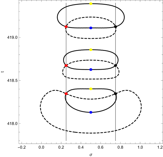
Figure 1: The black full lines denote contours $|{\cal W}(s)|=1$, while the black dashed lines denote contours $|{\cal V}(s)|=1$. Blue dots denote zeros of ${\cal V}(s)$, while yellow dots denote poles. Black dots denote zeros of ${\cal U}(s)$, while red dots denote poles. The Riemann hypothesis locates zeros of ${\cal U}(s)$ on $\sigma=3/4$, and poles on $\sigma=1/4$.

What is evident in Fig. 1 is that zeros and poles of ${\cal U}(s)$ sit between zeros and poles of ${\cal V}(s)$ on contours $|{\cal W}(s)|=1$, with the former lying where $|{\cal W}(s)|=1$ intersects $|{\cal V}(s)|=1$. These properties are important, because they establish a one-to-one correspondence between zeros of ${\cal V}(s)$ or ${\cal W}(s)$ and those of ${\cal U}(s)$. As remarked, we know that the density function of the first is that corresponding to that of the zeros of ${\cal U}(s)$ everywhere in $0<\sigma<1$ . However, zeros of ${\cal U}(s)$ off the line $\sigma=3/4$ occur not singly, but in pairs, so that such pairs must be sufficiently rare to not disturb the distribution function. Hence, we can deduce from Fig. 1, if the geometry shown holds for all zeros of ${\cal W}(s)$, then almost all zeros of ${\cal U}(s)$ lie on the line $\sigma=3/4$. We also know that zeros of ${\cal U}(s)$ lying on a contour $|{\cal W}(s)|=1$ which has a simple zero of ${\cal W}(s)$ at its centre must also be simple. Hence, we further deduce that almost all zeros of ${\cal U}(s)$ are simple.

It is one purpose of the remainder of this paper to unite known results and new results in order to show that Fig. 1 represents a universal behaviour.

3 Properties of Combinations of Zeta Functions

In this section, we review the properties of combinations of $\xi$ functions and their zeros, which will be needed for the arguments presented in Section 3.

3.1 The Results of Taylor

The posthumous paper of P.R. Taylor contains results on five related topics, only the first of which is of interest here. The following result is proved:

Theorem 1.

(Taylor) The function $f(s)=\xi_{1}(s+1/2)-\xi_{1}(s-1/2)$, odd under $s\rightarrow 1-s$, has all its complex zeros on $\sigma=1/2$.

Taylor’s proof examines using the argument principle the difference between the number of zeros in the critical strip and on the critical line with $0<t<T$, and bounding the difference in such a way as to give the result.

3.2 The Results of Lagarias and Suzuki

The substantial paper by Lagarias and Suzuki [7] was written at around the same time as that of Ki [8]. Although the two papers overlap in some results, there are results in both we will need for the arguments of Section 3.

The main theorems proved by Lagarias and Suzuki are now given, using our notations.

Theorem 2.

(Lagarias and Suzuki )

The meromorphic function, even under $s\rightarrow 1-s$,

$$\xi_{1}(2s)\frac{1}{s-1}-\xi_{1}(2s-1)\frac{1}{s}$$ (8)

has all its zeros on the critical line.

The next result quoted is for a more general function, again even under $s\rightarrow 1-s$:

Theorem 3.

(Lagarias and Suzuki )

For each fixed $T\geq 1$, the meromorphic function

$$I(T,s)=-\xi_{1}(2s)\frac{T^{s-1}}{s-1}+\xi_{1}(2-2s)\frac{T^{-s}}{s}$$ (9)

has all its zeros on the critical line.

The third example is motivated by an Eisenstein series result, commonly viewed as due to Chowla and Selberg [11], but in its essence predated by a paper of H. Kober [12]. Kober’s equation (5a) is:

$$(ac-b^{2})^{s/2-1/4}a^{1/2}\frac{\Gamma(s)}{8\pi^{s}}\sum_{(m_{1},m_{2})\neq(0,0)}\frac{1}{(am_{1}^{2}+2bm_{1}m_{2}+cm_{2}^{2})^{s}}$$

$$=\frac{1}{4}u^{-(s-1/2)}\xi_{1}(2s-1)+\frac{1}{4}u^{(s-1/2)}\xi_{1}(2s)$$

$$+\sum_{m_{1},m_{2}=1,\infty}\left(\frac{m_{1}}{m_{2}}\right)^{(s-1/2)}K_{s-1/2}(2\pi um_{1}m_{2})\cos(2\pi vm_{1}m_{2}),$$ (10)

where $v=b/a$ and $u^{2}+v^{2}=c/a$. The double sum on the left-hand side runs over all pairs of positive or negative integers, excluding the origin. This sum has been well studied, with the aim of discovering for what special values of $a$, $b$ and $c$ it can be represented as a finite superposition of products of Dirichlet $L$ functions- see Table 1.6 of Borwein et al [9] for known results. In general, if more than one Dirichlet $L$ product appears in the result for a sum, it will have non-trivial zeros off the critical line.

The Macdonald function sum on the right-hand side is rapidly convergent for the imaginary part of $s$ not large, but the region of summation required for accuracy increases linearly with the imaginary part. This sum can have zeros off the critical line [13].

The first term on the right-hand side has been studied by both Lagarias and Suzuki, and by Ki. Its zeros are governed in the following result:

Theorem 4.

(Lagarias and Suzuki) For each $y\geq 1$ the zeros of the function

$$a_{0}(y,s)=\xi_{1}(2s)y^{s}+\xi_{1}(2-2s)y^{1-s}$$ (11)

have the properties that, for $1\leq y\leq y^{*}=4\pi e^{-\gamma}\simeq 7.055507$ all zeros lie on the critical line, while for $y>y^{*}$ there are exactly two off the critical line and in the unit interval.

Let $N(f,T)$ count the number of zeros of the function $f(s)$ having $0\leq t\leq T$. Then Lagarias and Suzuki give the relationship between zero distributions of $a_{0}(y,s)$ and $\xi_{1}(2s)$:

$$N(a_{0}(y,s),T)=N(\xi_{1}(2s),T)+\frac{2}{\pi}\log(y)T+O(1),$$ (12)

where, from Titchmarsh and Heath-Brown [2], Theorem 9.4,

$$N(\xi_{1}(2s),T)=\frac{T}{\pi}\log T-\frac{T}{\pi}(\log\pi+1)+O(\log T).$$ (13)

Note that, from equation (12),

$$N(a_{0}(1,s),T)=N(\xi_{1}(2s),T)+O(1).$$ (14)

3.3 The Results of Ki

Ki proves results relating to the function

$$f(y,s)=(s-1)s(2s-1)\xi_{1}(2s)y^{s}+s(1-s)(1-2s)\xi_{1}(2-2s)y^{1-s},$$ (15)

which is odd under $y\rightarrow 1-s$. Then

Theorem 5.

(Ki) All complex zeros of $f(s)$ are simple and lie on the critical line.

For $y=1$ this reduces to Taylor’s result Theorem 1.

Another valuable set of results relate to the following function:

$$\theta(t)=\arg[(2it)(1/2+it)(-1/2+it)\xi_{1}(1+2it)].$$ (16)

Then:

Lemma 1.

(Ki) The function $\theta(t)$ has the properties: (1) $\theta(0)=\pi$, (2) $\theta(t)>\pi/2$ for $t>0$, (3) $\theta(t)$ is a convex function in $(0,7)$ and (4) $\theta(t)$ increases in $[7,\infty)$, with $\theta^{\prime}(t)\sim\log t$.

3.4 The Functions ${\cal T}_{+}(s)$ and ${\cal T}_{-}(s)$

We continue with two discussions related to functions for which it is known that all non-trivial zeros are first-order and located on the critical line [8, 7, 14].

The first function is defined as:

$${\cal T}_{+}(s)=\frac{1}{4}[\xi_{1}(2s)+\xi_{1}(2s-1)].$$ (17)

It has a pole of order unity at $s=0$:

$${\cal T}_{+}(s)\sim-\frac{1}{8s}+\frac{1}{24}(3\gamma+\pi-3\log(4\pi))+O(s).$$ (18)

It tends to a constant at $s=1/2$:

$${\cal T}_{+}(s)\sim\frac{1}{4}(\gamma-\log(4\pi))+O((s-1/2)^{2}).$$ (19)

It has a pole of order unity at $s=1$:

$${\cal T}_{+}(s)\sim\frac{1}{8(s-1)}+\frac{1}{24}(3\gamma+\pi-3\log(4\pi))+O(s-1).$$ (20)

It is even under $s\rightarrow 1-s$.

The function ${\cal T}_{+}(s)$ takes the following form on the critical line:

$${\cal T}_{+}(1/2+it)=2|\xi_{1}(1+2it)|\cos[\arg(\xi_{1}(1+2it)|],$$ (21)

and thus its zeros correspond to $\arg(\xi_{1}(1+2it)=(n+1/2)\pi$ for any integer $n$.

The author has compiled a list of the first 1517 zeros of ${\cal T}_{+}(s)$, the last of which is at $t=\Re(s)\simeq 999.912$. (A list of the first 1517 zeros of ${\cal T}_{+}(s)$ is available via the electronic supplementary material to this paper.)

The second function is defined as:

$${\cal T}_{-}(s)=\frac{1}{4}[\xi_{1}(2s)-\xi_{1}(2s-1)].$$ (22)

This function is odd under $s\rightarrow 1-s$. It has poles at $s=0$, $s=1/2$ and $s=1$, and zeros on the real line at $s=3.91231$ and $s=-2.91231$. The function ${\cal T}_{-}(s)$ takes the following form on the critical line:

$${\cal T}_{-}(1/2+it)=2i|\xi_{1}(1+2it)|\sin[\arg(\xi_{1}(1+2it)|],$$ (23)

and thus its zeros correspond to $\arg(\xi_{1}(1+2it)=n\pi$ for any integer $n$.

Once again, a list of the first 1517 zeros of ${\cal T}_{-}(s)$ is available via the electronic supplementary material to this paper.

Let

$$\theta_{1}(t)=\arg[\xi_{1}(1+2it)].$$ (24)

Then, from (16), in $t>0$,

$$\theta(t)=-\frac{\pi}{2}+\theta_{1}(t),$$ (25)

and

$$\theta^{\prime}(t)=\theta_{1}^{\prime}(t).$$ (26)

In so far as the properties of ${\cal T}_{+}(s)$ and ${\cal T}_{-}(s)$ are concerned, these are collected in the following Theorem:

Theorem 6.

The functions ${\cal T}_{+}(s)$ and ${\cal T}_{-}(s)$ have all their complex zeros on the critical line, and they occur in interlaced fashion, with a zero of the former lying between zeros of the latter, and vice versa. All zeros of each are simple, and the distribution functions of each satisfy:

$$N({\cal T}_{+}(s),T)=N({\cal T}_{-}(s),T)=N(\xi_{1}(2s),T)=\frac{T}{\pi}\log T-\frac{T}{\pi}(\log\pi+1)+O(\log T).$$ (27)

Proof.

These statements follow from the results of Taylor, Suzuki and Lagarias, and Ki, as well as from equation (26). The first complex zero of ${\cal T}_{+}(s)$ occurs for $t\simeq 6.97468$, while that for ${\cal T}_{-}(s)$ occurs for $t\simeq 7.66111$, after which the interlacing property commences. We emphasise that in equation (27) the zeros counted all lie on the critical line for the first two functions, but for the third the zeros referred to lie in $0<\sigma<1/2$. ∎

It is interesting to investigate whether a positional relationship exists between the zeros of either ${\cal T}_{+}(s)$ or ${\cal T}_{-}(s)$ and those of $\xi_{1}(2s-1/2)$, which under the Riemann hypothesis all lie on the critical line. We have investigated firstly whether zeros of $\xi_{1}(2s-1/2)$ all lie after those of ${\cal T}_{+}(s)$. In fact, of the first 1500 zeros of the latter, this property does not hold in 232 or 15.5% of cases. We can also ask whether numbered zeros of $\xi_{1}(2s-1/2)$ lie between successive zeros of ${\cal T}_{-}(s)$. This property fails only in four cases: 921, 995, 1307 and 1495. Using translations we can make the property hold for all 1500 zeros: translations by $s_{0}=it_{0}$ achieve this for $t_{0}$ in the range -0.080 to -0.036. This same translation along the critical line leads to a variation along it of the shifted ratio ${\cal T}_{+}(s)/{\cal T}_{-}(s)$ of the form

$$\frac{{\cal T}_{+}(1/2+i(t-t_{0}))}{{\cal T}_{-}(1/2+i(t-t_{0}))}=-i\cot[\arg\xi_{1}(1+2i(t-t_{0}))].$$ (28)

Hence, each point on the critical line can be made a zero of either the numerator or the denominator function in (28). In addition, each zero of $\xi_{1}(2s-1/2)$ on the critical line can be made to coincide with a zero of ${\cal T}_{-}(s-s_{0})$ or of ${\cal T}_{+}(s-s_{0})$, or to lie between two such.

3.5 Properties of ${\cal V}(s)$ and ${\cal W}(s)$

From the functions ${\cal T}_{+}(s)$ and ${\cal T}_{-}(s)$ we construct two further functions:

$${\cal V}(s)=\frac{{\cal T}_{+}(s)}{{\cal T}_{-}(s)}=\frac{1+{\cal U}(s)}{1-{\cal U}(s)},$$ (29)

Note that

$${\cal V}(s)=\frac{1+\sqrt{\pi}\Gamma(s-1/2)\zeta(2s-1)/(\Gamma(s)\zeta(2s))}{1-\sqrt{\pi}\Gamma(s-1/2)\zeta(2s-1)/(\Gamma(s)\zeta(2s))},$$ (30)

leading to the first-order estimate for $|{\cal V}(s)|$ for $1<<|\sigma|<<t$

$$|{\cal V}(s)|\sim 1+\sqrt{\frac{2}{t}}.$$ (31)

The corresponding argument estimate in $1<<\sigma<<t$ is

$$\arg[{\cal V}(s)]\sim-\sqrt{\frac{2\pi}{t}}.$$ (32)

For ${\cal U}(s)$, we have

$${\cal U}(s)=\sqrt{\frac{\pi}{s}}(1+\frac{3}{8s}+\ldots)(1+\frac{1}{4^{s}}+\frac{2}{9^{s}}+\ldots).$$ (33)

From this, if $t>>1$ and $\sigma>2$ say, $|{\cal U}(s)|\sim\sqrt{\frac{2}{t}}$ and $\arg{\cal U}(s)$ lies in the fourth quadrant. The leading terms in the expansion for ${\cal V}(s)$ are

$${\cal V}(s)\sim 1+\sqrt{\frac{2}{t}}(1-i\sqrt{\pi})+O(1/t),$$ (34)

which places its argument in the fourth quadrant, close to the real axis. For ${\cal W}(s)$ we have

$${\cal W}(s)\sim-i+\sqrt{\frac{2}{t}}(1-i\sqrt{\pi})+O(1/t),$$ (35)

which places its argument in the fourth quadrant, close to the boundary with the third quadrant .

We know that ${\cal V}(s)$ has all its non-trivial zeros and poles interlaced along the critical line, while the Riemann hypothesis is that ${\cal U}(s)$ has its zeros on $\Re(s)=3/4$ and its poles on $\Re(s)=1/4$. From (29), zeros of ${\cal U}(s)$ correspond to ${\cal V}(s)=1$ and poles to ${\cal V}(s)=-1$. Both then must lie on contours of constant modulus $|{\cal V}(s)|=1$, which correspond to ${\cal U}(s)$ being pure imaginary: $\Re[{\cal U}(s)]=0$.

An investigation has been carried out into the relationship between the contours of constant modulus $|{\cal V}(s)|=1$ and the location of the zeros and poles of ${\cal U}(s)$, for the first 1500 zeros of ${\cal T}_{+}(s)$ and ${\cal T}_{-}(s)$. A convenient way of doing this in the symbolic/numerical/graphical package Mathematica is to use the option RegionPlot, and in this case to construct the regions in which $|{\cal V}(s)|\leq 1$, or equivalently in which $\Re[{\cal U}(s)]<0$. These can be combined with contour plots of $|{\cal V}(s)|$, with contours appropriately chosen to highlight the location and behaviour around zeros of the derivative function ${\cal U}^{\prime}(s)$, evaluated by numerical differentiation.

The results of this (rather labour intensive) investigation are quite suggestive. In each of the 1500 cases, a zero of ${\cal T}_{+}(s)$ on the critical line sits at the centre of a simply-connected region, whose boundary fully encloses the region $|{\cal V}(s)|\leq 1$. The region $|{\cal V}(s)|>1$ is multiply connected, in keeping with the estimate in equation (30) for $\sigma$ not too close to the critical line. Two examples are given in Figs. 2 and 3. The first example (zero 518 of ${\cal T}_{+}(s)$) shows what may be described as typical behaviour, while the second (zero 1495) corresponds to one of the four exceptions mentioned in the previous section.

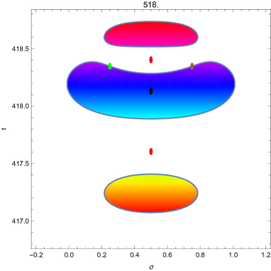
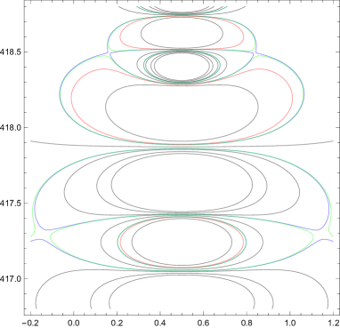
Figure 2: At left, three successive regions (coloured) in which $|{\cal V}(\sigma+it)|\leq 1$ are shown. Black dots represent zeros, red dots poles, while green and brown dots denote zeros of $\xi_{1}(2s)$ and $\xi_{1}(2s-1)$. At right, corresponding contours of constant modulus, with red denoting unit modulus, while green and blue contours correspond to moduli just above and below the values corresponding to the derivative zeros of ${\cal V}(\sigma+it)$.

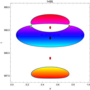
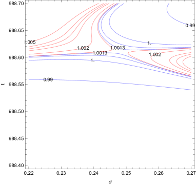
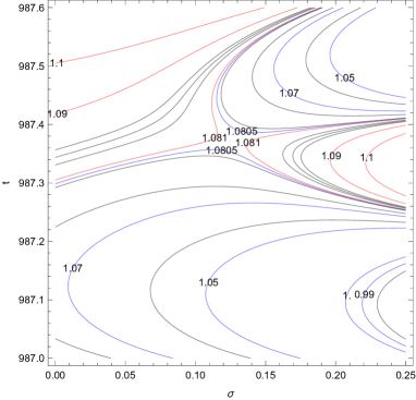
Figure 3: At left, three successive regions (coloured) in which $|{\cal V}(\sigma+it)|\leq 1$ are shown. Black dots represent zeros, red dots poles, while green and brown dots denote zeros of $\xi_{1}(2s)$ and $\xi_{1}(2s-1)$. At right, corresponding contours of constant modulus, showing the region around one of the derivative zeros of ${\cal V}(\sigma+it)$. Below: detail of contours of constant modulus in the region of the lower derivative zero.

In the first example, the contours of constant modulus shown are for the levels 0.90, 1.0, 1.018, 1.019, 1.1, 1.169, 1.170, 1.2, 1.3, 1.4. The zeros of ${\cal U}^{\prime}(s)$, or equivalently of ${\cal V}^{\prime}(s)$, are approximately $s=-0.143103+417.293i$, where $|{\cal V}(s)|=1.16957$, and $s=0.163301+418.4092i$, where $|{\cal V}(s)|=1.01891$. The upper derivative zero is defined by four contours of constant modulus, two in green provided by the zeros of ${\cal V}(s)$, and two in blue, one pertaining to the intervening pole of ${\cal V}(s)$ and the other to a closed curve enclosing the two poles and one zero. The lower structure is not complete as shown, but the outermost curve encloses two poles and an intervening zero.

In the second example, the zeros of ${\cal U}^{\prime}(s)$ are approximately $s=0.24809+988.611i$, where $|{\cal V}(s)|=1.001357$, and $s=0.12566+987.373i$, where $|{\cal V}(s)|=1.0808$. The structure near the upper derivative zero could be described as nearly closed, with the two contours of constant modulus coming close to touching. In consequence, the modulus at the derivative zero is much closer to unity than for the far more open structure around the lower derivative zero. For this example, both derivative zeros referred to are provided by two zeros of ${\cal V}(s)$ surrounding an intervening pole.

A nice geometrical insight into the results of this section comes from writing (29) in the normal form [15] already given in Section 2: see (7). This equation is built around the fixed points where ${\cal V}(s)=i={\cal U}(s)$ and ${\cal V}(s)=-i={\cal U}(s)$, which become the zeros and poles of ${\cal W}(s)$. Note that ${\cal W}(s)$ also incorporates the zeros and poles of ${\cal U}(s)$ and ${\cal V}(s)$:
the poles and zeros of ${\cal V}(s)$ are where ${\cal W}(s)=1$ and ${\cal W}(s)=-1$ respectively;
the poles and zeros of ${\cal U}(s)$ are where ${\cal W}(s)=i$ and ${\cal W}(s)=-i$ respectively.

Some further properties of ${\cal W}(s)$ are quoted next, taken from [14], starting with its functional equation:

$${\cal W}(1-s)=\frac{1}{{\cal W}(s)}.$$ (36)

It is real on the critical line, has unit modulus on the real axis, has the special values ${\cal W}(0)=-i$, ${\cal W}(1/2)=-1$, and in $t>>\sigma>>1$ has the asymptotic expansion

$${\cal W}(\sigma+it)=-i+(1-i)\sqrt{\frac{2\pi}{t}}+\frac{2\pi}{t}+(1+i)(\pi+\frac{\sigma}{2})\sqrt{\frac{2\pi}{t^{3}}}+\ldots.$$ (37)

All zeros and poles of ${\cal W}(s)$ lie on the critical line, and are interlaced:

$${\cal W}(1/2+it)=\tan[\arg(\xi_{1}(1+2it))+\frac{\pi}{4}].$$ (38)

Some properties of ${\cal W}(s)$ are exemplified in Fig. 4, and Table 1. Lines $|{\cal W}(s)|=1$ correspond to $\Im{\cal V}(s)=0$, which also correspond to $\Im{\cal U}(s)=0$. The lines of constant argument join at the zeros and poles of ${\cal W}(s)$, and cut $\sigma=1/2$ at zeros and poles of ${\cal V}(s)$, while cutting $\sigma=1/4,3/4$ at zeros and poles of ${\cal U}(s)$. Points where ${\cal W}^{\prime}(s)=0$ are also points where ${\cal U}^{\prime}(s)=0$ and ${\cal V}^{\prime}(s)=0$. In the example at right in Fig. 4, the derivative zero is located close to $\sigma=1/4$, but still to its left. Note also that in this case the concavity of the constant modulus curves means that the alternating property of zeros along these curves does not carry over to their $t$ values.

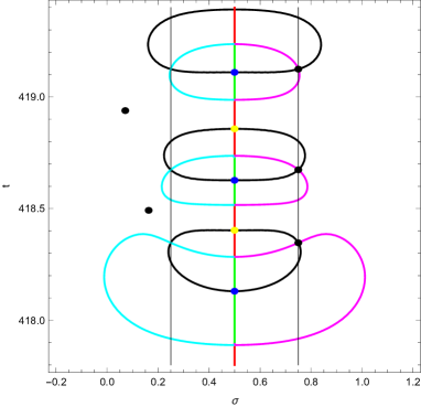
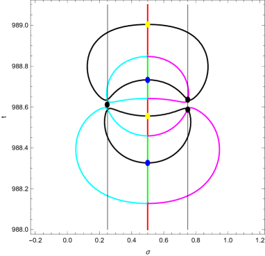
Figure 4: Contour plots showing (black lines) contours $|{\cal W}(s)|=1$. Coloured lines denote lines of constant argument of ${\cal W}(\sigma+it)$ as a function of $\sigma$ and $t$. The argument values are: $0$- red; $\pm\pi$- green, $\pi/2$-cyan; $-\pi/2$- magenta. The dots on $\sigma=1/2$ are zeros (blue) and poles (yellow) of ${\cal V}(s)$; those on $\sigma=3/4$ are zeros of ${\cal U}(s)$, with the corresponding poles being located symmetrically on $\sigma=1/4$. The other black dots show points where ${\cal W}^{\prime}(s)=0$.

It is easy to show that the equation $|{\cal V}(s)|=|{\cal W}(s)|$ has solutions if and only if ${\cal U}(s)=\Re({\cal U}(s))(1-i)$, which places $\arg{\cal U}(s)$ either in the second or fourth quadrants. The particular case where the common modulus is unity arises if and only if $\Re{\cal U}(s)=0=\Im{\cal U}(s)$.

Quadrant	Line	Quadrant
Q2	$|{\cal V}(s)|=1$	Q1
$|{\cal V}(s)|<1$,	$\arg{\cal U}(s)=\frac{\pi}{2}$	$|{\cal V}(s)|>1$,
$|{\cal W}(s)|<1$		$|{\cal W}(s)|<1$
$\arg{\cal U}(s)=\pm\pi$		$\arg{\cal U}(s)=0$
Q3	$|{\cal V}(s)|=1$	Q4
$|{\cal V}(s)|<1$,	$\arg{\cal U}(s)=-\frac{\pi}{2}$	$|{\cal V}(s)|>1$,
$|{\cal W}(s)|>1$		$|{\cal W}(s)|>1$
Boundaries	Properties
Q1-Q4:	$|{\cal W}(s)|=1$	$|{\cal V}(s)|>1$
Q1-Q2:	$|{\cal W}(s)|<1$	$|{\cal V}(s)|=1$
Q2-Q3:	$|{\cal W}(s)|=1$	$|{\cal V}(s)|<1$
Q3-Q4:	$|{\cal W}(s)|>1$	$|{\cal V}(s)|=1$
Diagonals	Properties
Q1	$\arg{\cal U}(s)=\pi/4$	$|{\cal V}(s)|=1/|{\cal W}(s)|$
Q2	$\arg{\cal U}(s)=3\pi/4$	$|{\cal V}(s)|=|{\cal W}(s)|$
Q3	$\arg{\cal U}(s)=-3\pi/4$	$|{\cal V}(s)|=1/|{\cal W}(s)|$
Q4	$\arg{\cal U}(s)=-\pi/4$	$|{\cal V}(s)|=|{\cal W}(s)|$

Table 1: Properties of ${\cal V}(s)$ and ${\cal W}(s)$ in the four quadrants of $\arg{\cal U}(s)$, on the lines separating them and on diagonals.

Given the triplet of functions ${\cal U}(s)$, ${\cal V}(s)$ and ${\cal W}(s)$, we can also construct relations other than (7) in normal form. That involving ${\cal U}(s)$ and ${\cal W}(s)$ is

$$\frac{{\cal W}(s)-1}{{\cal W}(s)+1}=i\left(\frac{{\cal U}(s)-1}{{\cal U}(s)+1}\right).$$ (39)

That involving ${\cal V}(s)$ and ${\cal W}(s)$ is more complicated. Let

$${\cal V}_{1}=\sqrt{2+\sqrt{3}}\exp[-i\pi/4],~{}{\cal V}_{2}=\sqrt{2-\sqrt{3}}\exp[i3\pi/4],~{}{\cal V}_{3}=-\frac{1}{2}+\frac{\sqrt{3}}{2}i.$$ (40)

Then the ${\cal W}$, ${\cal V}$ equation in normal form is

$$\frac{{\cal W}(s)-{\cal V}_{1}}{{\cal W}(s)-{\cal V}_{2}}={\cal V}_{3}\left(\frac{{\cal V}(s)-{\cal V}_{1}}{{\cal V}(s)-{\cal V}_{2}}\right).$$ (41)

4 Four Propositions

There exist in the extensive literature devoted to the Riemann hypothesis several relevant papers concerning the location of zeros of the derivative of the Riemann zeta function. An early example is the paper in German of A. Speiser [10], for which detailed comments exist in English [16]. Spieser states that the Riemann hypothesis is equivalent to the proposition that the non-trivial zeros of $\zeta^{\prime}(s)$ lie in $\sigma>1/2$, i.e. to the right of the critical line. Arias-de-Reyna comments that Speiser’s methods are ”between the proved and the acceptable”, and gives numerical examples illustrating Speiser’s reasoning. A further comment is that a flawless proof of a stronger result is that due to Levinson and Montgomery [17], which we now quote.

Theorem 7.

(Levinson and Montgomery) The Riemann hypothesis is equivalent to $\zeta^{\prime}(s)$ having no zeros in $0<\sigma<1/2$.

We now consider the equivalent statement for ${\cal U}(s)$ for $1/2<\sigma<3/4$. As a stimulus for this,we give in Fig. 5 graphs of $\arg{\cal U}(\sigma+it)$ for $\sigma=1/2$, $\sigma=3/4$ and $\sigma=0.753$. The notable point is that the argument decreases monotonically as $t$ increases for $\sigma=3/4$ (as it has been shown by Ki to do for $\sigma=1/2$), but for values in excess of $\sigma=3/4$ it is no longer monotonic, but contains segments in which it increases with $t$.

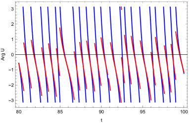
Figure 5: Plots of the argument of ${\cal U}(\sigma+it)$ for $\sigma=1/2$ (blue) and in red for (left) $\sigma=3/4$ and for (right) $\sigma=0.753$.

We will discuss this question in the context of four propositions, and discuss their relationships. In this section we will discuss the first two, and in the next the relationship between them and the second pair.

Proposition 1: All non-trivial zeros of ${\cal U}(s)$ lie on $\sigma=3/4$, and all non-trivial poles on $\sigma=1/4$.

Proposition 2: No zeros of ${\cal U}^{\prime}(s)$ or ${\cal V}^{\prime}(s)$ or ${\cal W}^{\prime}(s)$ lie between or on the lines $\sigma=3/4$ and $\sigma=1/4$.

Proposition 3: All non-trivial zeros of ${\cal U}^{\prime}(s)$ or ${\cal V}^{\prime}(s)$ or ${\cal W}^{\prime}(s)$ correspond to a modulus $|{\cal V}(s)|>1$.

Proposition 4: The values ${\cal V}(1/2+it)=i$ and ${\cal V}(1/2+it)=-i$ are attained by contours of constant $|{\cal V}(s)|$ increasing in modulus from zero.

Proposition 1 is of course the Riemann hypothesis.

4.1 Comments based on assuming Proposition 1

The following Theorem is an extension of a discussion in Section 4 of [14], and in particular of its Corollary 4.2.

Theorem 8.

If Proposition 1 holds, then $\Re\frac{\partial}{\partial s}\log{\cal U}(s)<0$ in $\frac{1}{4}\leq\sigma\leq\frac{3}{4}$ for $t>4.08046$.

Proof.

We let $s_{p}$ for $p$ integral run over all non-trivial poles of ${\cal U}(s)$ in $t>0$, which by assumption can be written $s_{p}=1/4+it_{p}$. The non-trivial zeros of ${\cal U}(s)$ are then located at $s_{p}+1/2=3/4+it_{p}$. Taking into account the zero and pole of ${\cal U}(s)$ on the real axis, we have the representation

$$\Re\frac{\partial}{\partial s}\log{\cal U}(s) = -\Re\left[\frac{1}{s-1}-\frac{1}{s}\right]-\sum_{p=1}^{\infty}m_{p}\Re\left[\frac{1}{s-s_{p}}-\frac{1}{s-1/2-s_{p}}\right]$$ (42)

$$-\sum_{p=1}^{\infty}m_{p}\Re\left[\frac{1}{s-{\bar{s}}_{p}}-\frac{1}{s-1/2-{\bar{s}}_{p}}\right].$$

Here the $m_{p}$ take into account possible zeros and poles of multiplicities exceeding unity. The equation (42) simplifies:

$$\Re\frac{\partial}{\partial s}\log{\cal U}(s) = -\Re\left[\frac{1}{s(s-1)}\right]+\frac{1}{2}\sum_{p=1}^{\infty}m_{p}\Re\left[\frac{1}{(s-s_{p})(s-1/2-s_{p})}\right]$$ (43)

$$+\frac{1}{2}\sum_{p=1}^{\infty}m_{p}\Re\left[\frac{1}{(s-{\bar{s}}_{p})(s-1/2-{\bar{s}}_{p})}\right].$$

We now substitute for $s_{p}$ as above and obtain, after identification of the real part,

$$\Re\frac{\partial}{\partial s}\log{\cal U}(s) = \left[\frac{\sigma(1-\sigma)+t^{2}}{(\sigma^{2}+t^{2})((1-\sigma)^{2}+t^{2})}\right]$$

$$+\frac{1}{2}\sum_{p=1}^{\infty}m_{p}\left[\frac{(\sigma-1/4)(\sigma-3/4)-(t-t_{p})^{2}}{((\sigma-1/4)^{2}+(t-t_{p})^{2})((\sigma-3/4)^{2}+(t-t_{p})^{2})}\right]$$

$$+\frac{1}{2}\sum_{p=1}^{\infty}m_{p}\left[\frac{(\sigma-1/4)(\sigma-3/4)-(t+t_{p})^{2}}{((\sigma-1/4)^{2}+(t+t_{p})^{2})((\sigma-3/4)^{2}+(t+t_{p})^{2})}\right].$$

The expression (LABEL:thm23-3) consists of two parts. The first is positive and converges as $1/t^{2}$ for $t$ large. Its expansion for $|t|$ large starts as $1/t^{2}$. The second has all of its terms negative if $1/4<\sigma<3/4$, and consists of two sums which converge quadratically as respectively $|t-t_{p}|$ and $|t+t_{p}|$ increase. Away from $\sigma=1/4$ and $\sigma=3/4$, we may expand the dominant elements of the second part to leading order as

$$-\frac{1}{2}\sum_{p=1}^{\infty}\left[\frac{1}{1/4+(t-t_{p})^{2}}+\frac{1}{1/4+(t+t_{p})^{2}}\right].$$ (45)

The second part is then readily seen to exceed the first part in modulus when $t$ is not small. This establishes the result in between the lines of zeros and poles.

Finally, consider the special case $\sigma=3/4$ (with a similar argument applying to $\sigma=1/4$) . Then we obtain

$$\Re\frac{\partial}{\partial s}\log{\cal U}(s)=\frac{3/16+t^{2}}{(9/16+t^{2})(1/16+t^{2})}-\frac{1}{2}\sum_{p=1}^{\infty}\left[\frac{1}{1/4+(t-t_{p})^{2}}+\frac{1}{1/4+(t+t_{p})^{2}}\right].$$ (46)

Numerically, the term $p=1$ in the sum has larger magnitude than the first term on the right-hand side when $t>4.08046$. ∎

Thus, Proposition 1 implies Proposition 2, and leads to an important result following immediately from Theorem 8:

Corollary 1.

If the Riemann hypothesis holds, then all zeros of $\zeta(s)$ on the critical line are simple.

Proof.

All zeros of $\zeta(s)$ for $t$ up to $O(10^{9})$ are known numerically to lie on the critical line, and to be simple. From the consideration of $\Re\frac{\partial}{\partial s}\log{\cal U}(s)$ on the lines $\sigma=3/4,1/4$,we know that ${\cal U}^{\prime}(s)$ has no zeros there. Taking into account the properties of the prefactor of $\zeta(2s-1)/\zeta(2s)$ in the expression (5) for ${\cal U}(s)$, this leads to the result. ∎

4.2 The equivalence of Propositions 1 and 2

To establish the equivalence of Propositions 1 and 2, we need the complementary statement: if Proposition 1 fails, then so does Proposition 2. To motivate the discussion of this, we multiply the function ${\cal V}(s)$ by a function which introduces an extra pair of zeros at $s_{\pm}=3/4\pm\delta+it_{*}$, together with appropriate balancing terms to preserve symmetry under $s\rightarrow 1-s$ and complex conjugation:

$${\cal F}(s,\delta,t_{*})=\frac{[s-(3/4+\delta+it_{*})][s-(3/4+\delta-it_{*})][s-(3/4-\delta+it_{*})][s-(3/4-\delta-it_{*})]}{[s-(1/4+\delta+it_{*})][s-(1/4+\delta-it_{*})][s-(1/4-\delta+it_{*})][s-(1/4-\delta-it_{*})]}.$$ (47)

We replace $s$ by $\sigma+it$, and define $\tilde{\sigma}=\sigma-3/4$, $\hat{\sigma}=\sigma-1/4=\tilde{\sigma}-1/2$, $t_{\pm}=t\pm t_{*}$. We then obtain:

$${\cal F}(\sigma,t,\delta,t_{*})=\frac{[(\tilde{\sigma}+it_{-})^{2}-\delta^{2}][(\tilde{\sigma}+it_{+})^{2}-\delta^{2}]}{[(\hat{\sigma}+it_{-})^{2}-\delta^{2}][(\hat{\sigma}+it_{+})^{2}-\delta^{2}]}.$$ (48)

We then define functions incorporating the zeros and poles off $\sigma=3/4$ and $\sigma=1/4$:

$${\cal U}_{oa}(s,\delta,t_{*})={\cal U}(s){\cal F}(s,\delta,t_{*}),$$ (49)

and

$${\cal V}_{oa}(s,\delta,t_{*})=\frac{1+{\cal U}_{oa}(s,\delta,t_{*})}{1-{\cal U}_{oa}(s,\delta,t_{*})},$$ (50)

$${\cal W}_{oa}(s,\delta,t_{*})=\frac{{\cal V}_{oa}(s,\delta,t_{*})-i}{{\cal V}_{oa}(s,\delta,t_{*})+i}.$$ (51)

The artificial example of this construction is given in Fig. 6, for the case $\delta=0.05$, $t_{*}=418.85$. There are closed contours of unit modulus as shown before in Fig. 4, together with new closed contours giving the inner zero and pole of ${\cal U}_{oa}(s,0.05,418.85)$, and open contours corresponding to its outer pole and zero. However, of most interest to this argument is the position of the derivative zero of ${\cal U}_{oa}$ at the point $0.737209+418.847i$ (together with another at $0.262791+418.847i$). This indicates a breakdown of Proposition 3 due to that of Proposition 2 in this artificial case.

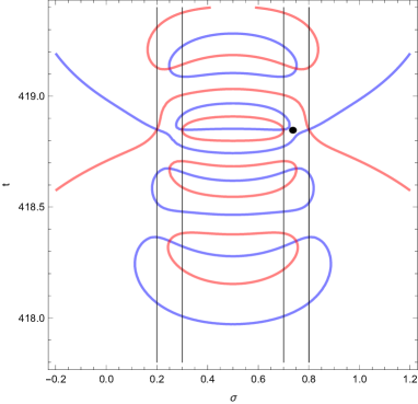
Figure 6: A contour plot showing (blue lines) contours $|{\cal W}_{oa}(s,0.05,0.418.85)|=1$ and (red lines) contours $|{\cal V}_{oa}(s,0.05,418.85)|=1$. Artificial poles and zeros have been introduced on the black lines $\sigma=0.20,0.30,0.70,0.80$, at positions where the red and blue contours intersect. Other zeros and poles are as in Fig. 4 (left).The black dot marks the position of a new derivative zero. Note that the new closed contour $|{\cal V}_{oa}(s,0.05,418.85)|=1$ is centred on a pole on the critical line near $t=418.853$.

Theorem 9.

If ${\cal U}(s)$ has zeros off $\sigma=3/4$ then ${\cal U}^{\prime}(s)$ has zeros between $\sigma=1/4$ and $\sigma=3/4$.

Proof.

We split the product representation of ${\cal U}(s)$ into a part with zeros and poles on $\sigma=3/4,1/4$ respectively, and a part which is a product of terms of the form (48), and with zeros and poles off $\sigma=3/4,1/4$:

$${\cal U}(s,\delta,t_{*})={\cal U}_{on}(s){\cal U}_{off}(s)={\cal U}_{on}(s)\prod_{q}{\cal F}(s,\delta_{q},t_{q}).$$ (52)

We can apply Theorem 8 to ${\cal U}_{on}(s)$, which is thus monotonic decreasing in modulus for non-small $t$ as $\sigma$ increases between $1/4$ and $3/4$.

As far as ${\cal U}_{off}(s)$ is concerned, let us take $q=1$ to be the case we are interested in investigating, where certainly $t_{1}^{*}$ is positive and very much larger than unity. Considering the term $q=1$ in isolation first, for $t$ close to $t_{1}$:

$${\cal F}(\sigma,t,\delta_{1},t_{1})=\frac{[(\tilde{\sigma}+it_{-})^{2}-\delta_{1}^{2}][(1-i\tilde{\sigma}/(2t_{1}))^{2}-\delta^{2}/(2t_{1})^{2}]}{[(\hat{\sigma}+it_{-})^{2}-\delta_{1}^{2}][(1-i\hat{\sigma}/(2t_{1}))^{2})-\delta^{2}/(2t_{1})^{2})]}.$$ (53)

This is zero when $\tilde{\sigma}=\pm 1/2$. Certainly $\delta_{1}<1/4$, so that the ratio of the second terms in the numerator and denominator in (53) can be replaced by unity when we look for the derivative zero on the line $t_{-}=0$ i.e. $t=t_{1}$. This derivative zero occurs when

$$2\tilde{\sigma}(\tilde{\sigma}^{2}+1/4+\tilde{\sigma}-\delta_{1}^{2})=(\tilde{\sigma}^{2}-\delta_{1}^{2})(2\tilde{\sigma}+1),$$ (54)

or

$$\tilde{\sigma}=-\frac{1}{4}(1\pm\sqrt{1-16\delta_{1}^{2}}\sim-2\delta_{1}^{2}.$$ (55)

It is natural that this should be $O(\delta_{1}^{2})$ since ${\cal F}$ is invariant under $\delta_{1}\rightarrow-\delta_{1}$. The derivative zero corresponds to a maximum modulus of this term.

The effect of the term ${\cal U}_{off}(s)$ is thus to move the derivative zero into the region $1/4<\sigma<3/4$. Since $|{\cal U}_{on}(s)|$ is monotonic decreasing for $\sigma$ increasing in this region, the effect of this term is to move the derivative zero of the modulus of the product further into the region, as well as to move it laterally off the line $t=t_{1}$ in general.

We must finally consider the effect of the possible terms $q\neq 1$ on the position of the derivative zero. Let $u_{q1}=t_{q}-t_{1}$. The effect of the term from $q$ is then a multiplicative factor

$$1+\frac{i/u_{q1}}{1-i/u_{q1}}\left(1+\frac{2(t-t_{1}-i\tilde{\sigma})/u_{q1}}{1-i/u_{q1}}\right),$$ (56)

which will not change the position of the derivative zero to leading order (since the leading order derivative contribution is independent of $\sigma$). ∎

Note that, in the artificial example in Fig. 6, the derivative zero of $|{\cal F}|$ occurs at $0.744949+415.85i$, giving a shift from the line $\sigma=3/4$ of $-0.005051$, agreeing well with $-2\delta_{1}^{2}$. The derivative zero of $|{\cal U}_{on}(s){\cal U}_{off}(s)|$ occurs at $0.737209+418.847i$, so the shift from the line $\sigma=3/4$ is $-0.01721$, with the movement due to $|{\cal U}_{on}(s)|$ exceeding that due to $\delta_{1}$.

5 Propositions 3 and 4

We commence with a result establishing a link between the equivalent Propositions 1, 2 and Proposition 3.

5.1 Comments based on Propositions 1 and 2

Theorem 10.

Propositions 1 and 2 imply Proposition 3.

Proof.

Given Propositions 1 and 2 hold, we wish to exclude the possibility that Proposition 3 does not hold. If this were the case, we would have an $s_{0}$ existing in $t_{0}>>1$ such that $|{\cal V}(s_{0})|<1$, where ${\cal V}^{\prime}(s_{0})=0$ . The contours of constant modulus of ${\cal V}(s)$ around its pertinent zero would then be limited to below $|{\cal V}(s_{0})|<1$, and thus would not reach the points ${\cal V}(s)=\pm i$ on the critical line. These then would have to be attained by a contour of constant modulus unity around the adjacent pole of ${\cal V}(s)$, which also passes through a zero of ${\cal U}(s)$ on the line $\sigma=3/4$. Further such contours then would have to exist ranging down in modulus towards $|{\cal V}(s_{0})|<1$, and cutting the line $\sigma=3/4$ with moduli smaller than unity before nearing $s_{0}$. This gives a contradiction, as $\sigma_{0}$ has to be above $\sigma=3/4$. ∎

5.2 The equivalence of Propositions 3 and 4

Remark: The only possible closed contours whose boundary is an equimodular contour of ${\cal V}(s)$ in $t$ not small cut the critical line twice. This is a simple consequence of the Maximum/Minimum Modulus Theorems, since the only non-trivial zeros and poles of ${\cal V}(s)$ lie on the critical line. Furthermore, contours of constant modulus touching the critical line are precluded since ${\cal V}^{\prime}(s)$ is never zero on the critical line.

Theorem 11.

Proposition 3 holds if and only if Proposition 4 holds.

Proof.

If Proposition 3 holds, then to each zero of ${\cal V}(s)$ on the critical line corresponds a set of contours of constant modulus, with that modulus able to increase until a zero of ${\cal V}^{\prime}(s)$ is encountered. As that zero must occur at a point where $|{\cal V}(s)|>1$, then the set of contours must include the contour of modulus unity. This intersects the critical line at the points ${\cal V}(s)=\pm i$.

Conversely, if Proposition 4 holds, then lines of constant modulus constructed around each zero must attain unity, where on the critical line ${\cal V}(s)=\pm i$. As there are no zeros of ${\cal V}^{\prime}(s)$ on the critical line, the set of lines of constant modulus must go beyond unity, showing that the relevant zero of ${\cal V}^{\prime}(s)$ corresponds to a modulus in excess of unity. ∎

Remark: If either of Propositions 3 and 4 fail, then there must exist contours of constant modulus based around a pole of ${\cal V}(s)$ attaining the relevant zero of ${\cal V}^{\prime}(s)$, at which the modulus of $|{\cal V}(s)|<1$.

Note that this situation occurs in the artificial example of Fig. 6. However, by the Theorems of this section, it cannot occur for ${\cal V}(s)$ in the range of $t$ for which the Riemann hypothesis is known to hold numerically.

5.3 From Proposition 3 towards Proposition 1

Theorem 12.

If Proposition 3 holds, then there exists a set of simple zeros of ${\cal U}(s)$ off the critical line in one-to-one correspondence with the zeros of ${\cal T}_{+}(s)$ on the critical line.

Proof.

The proof generalises the reasoning of Macdonald [18] to functions having poles and zeros. We note that $|{\cal V}(s)|=|{\cal V}(1-\overline{s})|$ is a symmetric function under reflection in the critical line, so curves of constant modulus share this property. Starting from a general zero of ${\cal T}_{+}(s)$, we constrain the family of closed curves on which its modulus is constant. This family of curves has as its final member that curve of constant modulus touching a zero of ${\cal V}^{\prime}(s)$, and so by the assumption of this Theorem the corresponding constant modulus exceeds unity. It then follows that there is a closed curve of constant modulus unity enclosing the zero of ${\cal T}_{+}(s)$. This closed curve intersects the critical line at points where ${\cal V}(s)={\cal U}(s)=\pm i$, and at every point on it ${\cal U}(s)$ is pure imaginary. The curve encloses one simple zero of ${\cal V}(s)$, and thus the argument of this function increases monotonically through a range of $2\pi$ along it, ensuring that it passes through $\pm 1$ upon it. On each such curve of constant modulus unity there is then a simple pole and a simple zero of ${\cal U}(s)$, establishing the one-to-one correspondence referred to in the Theorem statement. ∎

Corollary 2.

If Proposition 3 holds, then the distribution function for zeros of $\xi_{1}(2s-1/2)$ on the critical line with $0<t<T$ is given by (27).

Proof.

From Theorem 12, there exists for each zero of ${\cal T}_{+}(s)$ on the critical line a simple zero of ${\cal U}(s)$(i.e. of $\xi_{1}(2s-1)$) lying on the contour $|{\cal T}_{+}(s)/{\cal T}_{-}(s)|$ enclosing the zero of ${\cal T}_{+}(s)$. By Theorem 27 the distribution function for zeros of ${\cal T}_{+}(s)$ is the same as that for the number of zeros of $\xi_{1}(2s-1/2)$ lying in the strip $1/4<\sigma<3/4$ with $0<t<T$. If any such zero were to lie off the critical line, it would have to occur in a pair of zeros symmetric about the critical line. However, we have established that there exists the set of simple zeros of $\xi_{1}(2s)$ in precise 1:1 correspondence with the zeros of ${\cal T}_{+}(1/2+it)$. Hence, any zeros off the critical line would have to be sufficiently rare to leave the distribution function (27) unaltered. In other words, the distributions functions for zeros on the critical line of $\xi_{1}(2s-1/2)$, ${\cal T}_{+}(s)$ and ${\cal T}_{-}(s)$ are all the same and given by (27), if Theorem 12 holds. ∎

5.4 Proposition 3 and Topology

Theorem 13.

Assuming Proposition 3, to every closed contour $|{\cal V}(s)|=1$ around a zero of ${\cal V}(s)$ corresponds a closed contour $|{\cal W}(s)|=1$ around a zero of ${\cal W}(s)$.

Proof.

Given a closed contour $|{\cal V}(s)|=1$ around a point where ${\cal U}(s)=-1$. From Table 1, this consists of elements in quadrants $Q_{2}$ and $Q_{3}$ of $\arg{\cal U}(s)$ joined by a line $|{\cal W}(s)|=1$ where $\arg{\cal U}(s)=\pm\pi$. On the closed contour $|{\cal V}(s)|=1$ lie a zero and a pole of ${\cal U}(s)$. All four quadrants of $\arg{\cal U}(s)$ meet at the zero and pole of ${\cal U}(s)$. The area with ${\cal U}(s)$ in quadrant $Q_{2}$ is also a region where $|{\cal W}(s)|<1$. Outside the contour $|{\cal V}(s)|=1$ we have regions in $Q_{4}$ and $Q_{1}$, the former also being a region with $|{\cal W}(s)|>1$. The $Q_{1}$ region has $|{\cal W}(s)|<1$ and is joined to the $Q_{2}$ region along a contour $|{\cal V}(s)|=1$, $\arg{\cal U}(s)=\pi/2$. The desired region $|{\cal W}(s)|<1$ is then formed by the union of the $Q_{1}$, $Q_{2}$ regions. ∎

Corollary 3.

Given Proposition 3, then points where ${\cal W}^{\prime}(s)=0={\cal U}^{\prime}(s)={\cal V}^{\prime}(s)$ have $\arg{\cal U}(s)$ lying in the fourth quadrant.

Proof.

This follows directly from Theorem 13 and Table 1, given that regions $|{\cal V}(s)|\leq 1$ correspond to regions $|{\cal W}(s)|\leq 1$. ∎

Remark: From the arguments of this subsection, it is a consequence that to every zero of ${\cal T}_{+}(s)$ corresponds a region around it formed by the union of regions with $\arg{\cal U}(s)$ in the first, second and third quadrants, enclosed within a region with $\arg{\cal U}(s)$ in the fourth quadrant. It should be noted that the fourth quadrant region is simply connected, while the other three quadrants are found in island regions within the fourth quadrant region.

6 Supplementary Data

Data on the zeros up to $t=1000$ on the critical line of the functions ${\cal T}_{+}(s)$ and ${\cal T}_{+}(s)$ is available in the electronic supplementary material.

7 Acknowledgements

The author acknowledges gratefully contributions from colleagues (C.G. Poulton, L.C. Botten, the late N-A. Nicorovici) to previous published work which laid the foundations for what is reported here.

References

- [1] Edwards HM, 2001 Riemann’s Zeta Function, Mineola NY:Dover pp. 132-134.
- [2] Titchmarsh EC, Heath-Brown DR, 1986 The Theory of the Riemann Zeta-function, Oxford UK: Oxford .
- [3] Borwein, J. & Bailey, D. 2004. Mathematics by Experiment: Plausible Reasoning in the 21st Century,Natick, Mass: A.K. Peters. ISBN 978-1-56881-211-3.
- [4] Bohr, H. & Landau, E., 1914 Eine Satz über Dirichletsche Reihen mit Anwendung auf die -Funktion und die L-Funktionen Rend. di Palermo 37 269-72.
- [5] Bui, H.M., Conrey J.B. & Young, M.P. 2011 More than 41% of the zeros of the zeta function are on the critical line Acta Arith. 150 35-64.
- [6] Taylor, P.R. 1945 On the Riemann zeta-function, Q.J.O., 16, 1-21.
- [7] Lagarias, J.C. and Suzuki, M. 2006 The Riemann hypothesis for certain integrals of Eisenstein series J. Number Theory 118 98-122.
- [8] Ki H 2006 Zeros of the constant term in the Chowla-Selberg formula Acta Arithmetica 124 197-204.
- [9] Borwein JM, Glasser ML, McPhedran RC, Wan JG & Zucker IJ, 2013 Lattice Sums Then and Now, Cambridge UK: Cambridge.
- [10] Speiser, A. 1934 Geometrisches zur Riemannschen Zetafunktion, Math. Ann. 110 514 521.
- [11] Chowla S & Selberg A 1967 On Epstein’s zeta-function J. Reine Angeq. Math. 227 86-110.
- [12] Kober H 1935 Transformationsformeln gewisser Besselscher Reihen, Beziehungen zu Zeta-Funktionen Math. Z. 39 609-624.
- [13] McPhedran RC Smith GH Nicorovici NA & Botten LC 2004 Distributive and analytic properties of lattice sums JMathPhys 45, 2560-2578.
- [14] McPhedran, R.C. & Poulton, C.G. 2013 The Riemann Hypothesis for Symmetrised Combinations of Zeta Functions, arXiv:1308.5756.
- [15] Knopp, K., 1952 Elements of the Theory of Functions, Dover NY Chapter 5.
- [16] Arias-de-Reyna, J. 2003 X-ray of Riemann zeta-function,arXiv:2003.09433.
- [17] Levinson, N., & Montgomery, H. L. 1974 Zeros of the Derivatives of the Riemann Zeta-Function, Acta Math.133, 49 65.
- [18] McPhedran, R.C. 2017 Macdonald’s Theorem for Analytic Functions, arXiv:1702.03458.