Large-deviation properties of the largest biconnected component for random graphs

Abstract

We study the size of the largest biconnected components in sparse Erdős-Rényi graphs with finite connectivity and Barabási-Albert graphs with non-integer mean degree. Using a statistical-mechanics inspired Monte Carlo approach we obtain numerically the distributions for different sets of parameters over almost their whole support, especially down to the rare-event tails with probabilities far less than $10^{-100}$. This enables us to observe a qualitative difference in the behavior of the size of the largest biconnected component and the largest $2$-core in the region of very small components, which is unreachable using simple sampling methods. Also, we observe a convergence to a rate function even for small sizes, which is a hint that the large deviation principle holds for these distributions.

1 Introduction

The robustness of networks newman2003review ; dorogovtsev_book2006 ; newman_book2006 ; newman_book2010 ; barrat_book2012 attracted much interest in recent time, from practical applications for, e.g., power grids Sachtjen2000Disturbances ; Rohden2012self ; dewenter2015large , the internet Cohen2000Resilience ; lee2006maximum , to examinations of genomes ghim2005lethality ; kim2015biconnectivity . As typical in network science, one does not only study the properties of existing networks. To model the properties of real networks, different ensembles of random graphs were devised, e.g., Erdős-Rényi random graphs erdoes1960 , small world graphs watts1998 , or scale-free graphs barabasi1999emergence . Also for such ensembles the robustness has been studied by analytical and numerical means albert2000error ; Callaway2000network ; Newman2008Bicomponents ; Norrenbrock2016fragmentation . One often used approach to determine the robustness of networks are fragmentation studies, where single nodes are removed from the network. These nodes are selected according to specific rules (“attack”) or randomly (“failure”). The functionality, e.g., whether it is still connected, is tested afterwards. A property necessary for robustness is thus that the graph stays connected when removing an arbitrary node. This exact concept is characterized by the biconnected component, which are the connected components which stay connected after an arbitrary node is removed. The existence of a large biconnected component is thus a simple and fundamental property of a graph robust to fragmentation. Another, though related, often studied form of stability looks at the flow through or the transport capability lee2006maximum of a graph. Also here a large biconnected component is a good indicator for stability. Intuitively, in a biconnected component there is never a single bottleneck but always a backup path to reach any node. This ensures the function of the network even in case that an arbitrary edge has too low throughput or an arbitrary node of the biconnected component is damaged.

At the same time the biconnected component is a simple concept enabling to some extent its treatment by analytical means for some graph ensembles. For example, the mean size $\left<S_{2}\right>$ of the biconnected component for a graph with a given degree distribution is known Newman2008Bicomponents . Also the percolation transition of the biconnected component for scale free and Erdős-Rényi graphs is known to coincide with the percolation transition of the single connected component and its finite size scaling behavior is known Kim2013phase . Nevertheless, a full description of any random variable is only obtained if its full probability distribution is known. To our knowledge, concerning the size of the biconnected component this has not been achieved so far for any graph ensemble, neither analytically nor numerically.

For few network observables and some graphs ensembles results concerning the probability distributions have been already obtained so far. For the size of the connected component on Erdős-Rényi random graphs analytical results biskup2007large for the rate function exist, i.e., the behavior of the full distribution for large graph sizes $N$. Numerically it was shown that this is already for relatively small $N$ a very good approximation Hartmann2011large . Corresponding numerical results for two-dimensional percolation have been obtained as well Hartmann2011large . Similarly there are numerical, but no analytical works, scrutinizing the size of the related $2$-core over most of its support again for Erdős-Rényi random graphs Hartmann2017Large .

Since similar results seem not to be available concerning the biconnected components, and given its importance for network robustness, this is an omission that we will start to cure with this study. Here, we numerically obtain the probability density function of the size of the largest biconnected component over a large part of its support, i.e., down to probabilities smaller than $10^{-100}$. This enables us also to directly observe large deviation properties, and shows strong hints that the large deviation principle holds denHollander2000 ; touchette2009 for this distribution.

The remainder of this manuscript gives definitions of the graph ensembles and the properties of interest, as well as some known results, in section 2.1 and explains the sampling methods needed to explore the tails of the distributions in section 2.2. The results of our simulations and a discussion will follow in section 3. Section 4 summarizes the results.

2 Models and Methods

2.1 Biconnected Components of Random Graphs

A graph $G=(V,E)$ is a tuple of a set of nodes $V$ and edges $E\subset V^{(2)}$. A pair of nodes $i,j$ are called connected, if there exists a path of edges $\{i,i_{1}\},\{i_{1},i_{2}\},..,\{i_{k-1},i_{k}\},\{i_{k},j\}$ between them. A cycle is a closed path, i.e., the edge $\{i,j\}$ exists and $i$ and $j$ are connected in $G^{\prime}=(V,E\setminus\{i,j\})$. The connected components are the maximal disjoint subgraphs, such that all nodes of each subgraph are connected.

A biconnected component (sometimes bicomponent) of an undirected graph is a subgraph, such that every node can be reached by two paths, which are distinct in every node except the start- and end node. Thus, if any single node is removed from a biconnected component it will still be a connected component. Therefore clearly, each biconnected component is a connected component. We will also look shortly at bi-edge-connected components, which are very similar, but the two paths may share nodes as long as they do not share any edge. Note that a biconnected component is always a bi-edge-connected component, but the reverse is not necessarily true. An example is shown in Fig. 1. In this study we will study only the largest biconnected component $G_{\mathrm{bi}}$ of two types of random graphs. Note that, while every biconnected component is also a connected component, the largest biconnected component does not need to be a subgraph of the largest connected component $G_{\mathrm{cc}}$, it may be part of another, smaller, connected component. However, its size $S_{2}=|G_{\mathrm{bi}}|$ is always smaller or equal than the size of the largest connected component $S=\left|G_{\mathrm{cc}}\right|$. Similarly, the size $S_{\text{2-core}}$ of the largest connected component of the $2$-core, the subgraphs that remain after iterative removal of all nodes with degree less than $2$, is an upper bound on $S_{2}$, since the $2$-core of a graph consists of bicomponents possibly linked by single edges. In Fig. 1 the largest components of each type are visualized for an example connected graph. In fact for the sizes of the largest of the above introduced subgraphs, the following relation holds.

$$S\geq S_{\text{2-core}}\geq S_{\text{2-edge}}\geq S_{2}.$$ (1)

As we will see below, for the ensemble of Erdős-Rényi random graphs in the percolating phase, the distributions of $S_{\text{2-core}},S_{\text{2-edge}}$, and $S_{2}$ are actually very similar to each other. One has indeed to inspect the far tails of the distributions to see differences, which also justifies that we study the large-deviation properties here. For the ensemble of Barabási-Albert graphs we study, the same is true. While the distributions of $S_{\text{2-core}}$ and $S_{2}$ look very similar in the main region, a qualitative difference is observable in the tail of small components. The difference is even more pronounced than for the ER case, since the general form of the distribution changes qualitatively to a convex shape for $P(S_{\text{2-core}})$.

Figure 1: Every node is part of the connected component, nine nodes with bold borderline are part of the $2$-core, six nodes containing a circle are part of the largest bi-edge-connected component and all nodes containing a black dot are part of the largest biconnected component.

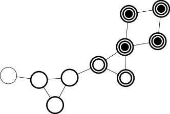
The classical way to find biconnected components of a graph Hopcroft1973algorithm is based on a depth first search and thus runs in linear time. For each connected component a depth first search is started at an arbitrary root node of that component. For each node the current depth of the search, i.e., at which level in the tree traversed by the depth first search the node is located, and the lowpoint are saved. The lowpoint is the minimum of the depth of the neighbors (in the graph) of all descendants of the node (in the tree). Iff the depth of a node is less or equal the lowpoint of one of its children (in the tree), this node separates two biconnected components and is called articulation point. For the root node of the search there is an exception. It is an articulation point, iff it has more than one child. The articulation points separate biconnected components and are members of all biconnected components separated by them. A better illustrated explanation can be found in cormen2009introduction . After finding all biconnected components, we measure the size of the largest. We did not implement an algorithm, instead we simply used the efficient implementation provided by the LEMON graph library lemon .

The mean size of the biconnected component of graphs with a given degree distribution $p_{k}$ is known for large graphs Newman2008Bicomponents ; ghoshal2009structural to be

$$\left<S_{2}\right>=1-G_{0}(u)-(1-u)G_{0}^{\prime}(u),$$ (2)

where $G_{0}(z)=\sum_{k}p_{k}z^{k}$ is the probability generating function, $G_{0}^{\prime}$ its derivative and $u$ the probability to reach a node not part of the giant connected component when following an edge. $u$ is determined by the solution of

$$u=\sum_{k=0}^{\infty}q_{k}u^{k},$$ (3)

with the excess degree distribution $q_{k}=(k+1)p_{k+1}/\left<k\right>$. Knowing the degree distribution of Erdős-Rényi graphs $G(N,p)$ to be

$$p_{k}=\binom{N-1}{k}p^{k}(1-p)^{N-1-k},$$ (4)

allows the numerical evaluation of Eq. (3). We will compare these predictions to our simulational results to scrutinize the behavior for finite $N$.

The ensemble of Erdős-Rényi (ER) graphs $G(N,p)$ consists of $N$ nodes and each of the $N(N-1)/2$ possible edges occurs with probability $p$. The connectivity $c=Np$ is the average number of incident edges per node, the average degree. At $c_{c}=1$ this ensemble shows a percolation transition. That is in the limit of large graph sizes $N$ the size of the largest connected component is of order $\mathcal{O}(N)$ above this threshold and of order $\mathcal{O}(1)$ below. Interestingly this point is also the percolation transition of the biconnected component Kim2013phase .

To a lesser extend we also study Barabási-Albert (BA) graphs barabasi1999emergence . The ensemble of BA graphs is characterized by a tunable mean degree $\left<k\right>$ and its degree distribution follows a powerlaw $p(k)\propto k^{-3}$. Realizations are constructed using a growth process. Starting from a fully connected subgraph of $m_{0}$ (here $m_{0}=3$) nodes, in every iteration one more node is added and connected to $m\leq m_{0}$ existing nodes $j$ with a probability $p_{j}\propto k_{j}$ dependent on their degree $k_{j}$ until the size of the graph is $N$. The parameter $m=2\left<k\right>$ by construction. Since $m=1$ will always result in a tree, which is not biconnected at all and $m\geq 2$ will always be a full biconnected component, we will allow fractional $1<m<2$ in the sense, that one edge is always added and a second with probability $m-1$.

2.2 Sampling

Since we are interested in the far tail behavior of the distribution of the size of the largest biconnected component, it is unfeasible to use naive simple sampling, i.e., uniformly generating configurations, measuring the observable and constructing a histogram. Instead we use a Markov chain Monte Carlo based importance sampling scheme to collect good statistics also in the far tails. This technique was already applied to obtain the distributions over a large range for the score of sequence alignments Hartmann2002Sampling ; Wolfsheimer2007local ; Fieth2016score , to obtain statistics of the convex hulls of a wide range of types of random walks Claussen2015Convex ; Dewenter2016Convex ; schawe2018avoiding ; schawe2018large , to work distributions for non-equilibrium systems Hartmann2014high and especially to different properties of Erdős-Rényi random graphs Engel2004 ; Hartmann2011large ; Hartmann2017Large ; hartmann2018distribution .

The Markov chain in this case is a chain of random number vectors $\bm{\xi}_{t}$, $t=1,2,\ldots$. Each entry of $\bm{\xi}_{t}$ is drawn from a uniform $U(0,1)$ distribution. Each vector serves as an input for a function which generates a random graph. Since all randomness is included in $\bm{\xi}_{t}$, the generated graph $G_{t}=G(\bm{\xi}_{t})$ depends deterministically on $\bm{\xi}_{t}$. In this way, the Markov chain $\{\bm{\xi}_{t}\}$ corresponds to a Markov chain $\{G_{t}\}$ of graphs. This approach, of separating the randomness from the actually generated objects, has the advantage that for the Markov chain we can generate graph realizations of arbitrary ensembles from scratch, without having to invent a valid Markov chain change move for each ensemble. However, for Erdős-Rényi graphs, we use a specialized change move for performance reasons. One change move is to select a random node $i$, delete all incident edges and add every edge $\{i,j\}$ with $j\in V\setminus\{i\}$ with probability $p$. For the Barabási-Albert graphs such a simple change move is not trivial to construct. Therefore, for this type, we perform the typical growth process from scratch after changing one of the underlying random numbers in $\bm{\xi}_{t}$.

Figure 2: Four steps of our importance sampling scheme at a small negative temperature, biasing towards a larger biconnected component.

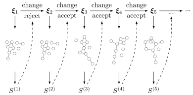
The main idea to obtain good statistics over a large part of the support, especially for probabilities smaller than, say, $10^{-100}$, is to bias the generated samples towards those regions. Therefore, we will use classical Metropolis sampling to gather realizations of graphs $G$. The Markov chain underlying this method consists of either Graph realizations $G$ (ER case) or random number vectors $\bm{\xi}$ from which a graph realization can be constructed $G(\bm{\xi})$ (BA case). We will describe the process for the latter more general case. We start our Markov chain with some random state $\bm{\xi}_{1}$ and at every iteration we propose a new state $\bm{\xi}^{\prime}$, i.e., replace a single entry of $\bm{\xi}_{t}$ with a new uniform random number and generate a new realization $G(\bm{\xi}^{\prime})$ from these random numbers. We will accept this proposal as the new state $\bm{\xi}_{i+1}$, with the classical Metropolis acceptance probability $p_{\mathrm{acc}}=\min\{1,\operatorname{e}^{-\Delta S/T}\}.$ This process is sketched in Fig. 2. Since we are interested in the size of the largest biconnected component $S$, we will treat this observable as the “energy” of the realization. Thus, $\Delta S$ is the difference in energy between the old and proposed state. Otherwise the proposal is rejected, i.e., $\bm{\xi}_{t+1}=\bm{\xi}_{t}$. Following this protocol, the Markov chain will equilibrate eventually and from thereon yield realizations $G(\bm{\xi})$ which are Boltzmann distributed with respect to some “artificial temperature” $T$

$$Q_{T}(G)=\frac{1}{Z_{T}}\operatorname{e}^{-S(G)/T}Q(G),$$ (5)

where $Q(G)$ is the natural distribution of the realizations and $Z_{T}$ the partition function, i.e., a normalization constant. Now, we can use the temperature $T$ as a tuning parameter to adjust the part of the distribution we want to gather samples from. Low positive temperatures will bias the “energy” $S$ towards smaller values because decreases in $S$ are always accepted and increases in $S$ are more often rejected. For negative $T$ this bias works in the opposite way towards larger values of $S$, i.e., larger biconnected components in this case.

For any chosen temperature, the sampling will be restricted to some interval determined by the value of $T$. Thus, to obtain the desired distribution $P(S)$ over a large range of the support, simulations for many different temperatures have to be performed. We have to choose the temperatures $T$ in a certain way, to be able to reconstruct the wanted distribution $P(S)$ from this data. First, we can transform $Q(G)$ into $P(S)$ by summing all realizations $G$, which have the same $S$. Hence we obtain with Eq. 5

$$P_{T}(S) =\sum_{\{G|S(G)=S\}}Q_{T}(G)$$

$$=\sum_{\{G|S(G)=S\}}\frac{\exp(-S/T)}{Z_{T}}Q(G)$$

$$=\frac{\exp(-S/T)}{Z_{T}}P(S).$$

With this relation we can calculate the wanted, unbiased distribution $P(S)$ from measurements of our biased distributions $P_{T}(S)$. The ratios of all constants $Z_{T}$ can be obtained by enforcing continuity of the distribution $P(S)$, i.e.,

$$P_{T_{j}}(S)\operatorname{e}^{S/T_{j}}Z_{T_{j}}=P_{T_{i}}(S)\operatorname{e}^{S/T_{i}}Z_{T_{i}}.$$

This requires that our measurements for $P_{T}(S)$ are at least pairwise overlapping such that there is no unsampled region between sampled regions. From pairwise overlaps the pairwise ratios $Z_{i}/Z_{j}$ can be approximated. The absolute value of the $Z_{T}$ can afterwards be obtained by the normalization of $P(S)$. Although the size of the largest biconnected component $S_{2}$ is a discrete variable for every finite $N$ and should therefore be normalized such that the probabilities of every event should sum to one, i.e., $\sum_{i=0}^{N}p(S_{2}=i/N)=1$, we are mainly interested in the large $N$ behavior and especially the rate function. This limit is continuous and should therefore be treated with a different normalization $\int_{0}^{1}p(S_{2})\,\mathrm{d}S_{2}=1$, which we approximate for finite $N$ by the trapzoidal rule. Anyway, the difference here is just a factor $N$.

While this technique does usually work quite well and all distributions but one exception are obtained with this method, there are sometimes first order phase transitions within the finite temperature ensemble, rendering it infeasible, or at least very tedious, to acquire values inbetween two temperatures. This was a problem here for the modified Barabási-Albert graph at the largest simulated graph size $N$. This phenomenon is well known and explored in detail in Hartmann2011large . We filled this gap by modified Wang-Landau simulations Wang2001Efficient ; Wang2001Determining ; Schulz2003Avoiding ; Belardinelli2007Fast ; Belardinelli2007theoretical with subsequent entropic sampling Lee1993Entropic ; Dickman2011Complete .

3 Results

We applied the temperature-based sampling scheme to ER with finite connectivities of $c\in\{0.5,1,2\}$ and BA with $m=1.3$ over practically the whole support $S_{2}\in[0,1]$ using around a dozen different temperatures for each ensemble and Markov chains of length $10^{6}N$ to gather enough samples after equilibration and discarding correlated samples. Additionally for BA the range $S_{2}\in[0.1,0.35]$ was sampled using Wang-Landau’s method and merged into results obtained from the temperature based sampling for the remainder of the distribution. All error estimates for the distributions are obtained via bootstrap resampling efron1979 ; young2015 but are always smaller than the symbol size and therefore not shown. Error estimates for fits are Gnuplot’s asymptotic standard errors.

Figure 3: Distributions of the size of the largest biconnected component $S_{2}$ for ER graphs at connectivity $c=2$ and three different graph sizes $N$. The main plot shows the distributions in logarithmic scale to display the tails, the inset shows the same distributions in linear scale, where a concentration around the mean value $\left<S_{2}\right>$ (cf. Fig 4) is visible. (For clarity not every bin is visualized.)

Examples for the distribution of the largest biconnected component’s size for ER graphs at $c=2.0$ are depicted in Fig. 3 at three different graph sizes $N$. The inset shows the distribution in linear scale, where a concentration with increasing size $N$ around the mean value is visible. While the main part of the distribution in the inset looks rather symmetric, the tails are obviously not. Also it is visible that the tails of the distribution get more and more suppressed when increasing the value of $N$.

Figure 4: Mean size of the largest biconnected component $\left<S_{2}\right>$ for different graph sizes $N$. Notice the broken $\left<S_{2}\right>$-axis. The black line denotes the analytic expectation for $c=2$ from Eq. 2 Newman2008Bicomponents . The expectation for $c\leq 1$ is $\left<S_{2}\right>=0$. Fits to a power law with offset $\left<S_{2}\right>=aN^{b}+S_{2}^{\infty}$ lead to $S_{2}^{\infty}=-6(8)\cdot 10^{-6}$ for $c=0.5$, $S_{2}^{\infty}=-0.0013(4)$ for $c=1.0$ and $S_{2}^{\infty}=0.4729(3)$ for $c=2.0$.

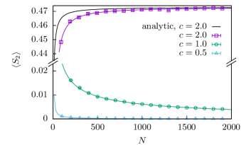
Since the mean size of the biconnected component of ER is known for large enough graphs, we will compare the mean sizes of our simulations to the analytical expectation. Those results are shown in Fig. 4, notice the broken $\left<S_{2}\right>$-axis. Apparently at $c=2$ for small sizes $N$ the analytical approximation, while close to our measurements, overestimates the size of the biconnected component slightly but the relative error diminishes for larger sizes. In fact, we extrapolated our measurements to the limit of large $N$ using a power-law ansatz $\left<S_{2}\right>=aN^{b}+S_{2}^{\infty}$ yielding for $c=0.5$ an offset $S_{2}^{\infty}$ compatible within errorbars with the expectation $\left<S_{2}\right>=0$ (exact values in the caption of Fig. 4), which is quite remarkable for our ad-hoc fit function. The case $c=1$ suggests a negative $S_{2}^{\infty}$ close to zero, which is probably caused by correction to our assumed scaling law. The case $c=2$ seems to converge to the limit of the analytical expectation also.

Figure 5: Comparison of the relative size of the largest connected component $S$ Hartmann2011large , the largest $2$-core $S_{\text{2-core}}$ Hartmann2017Large , the largest bi-edge-connected component $S_{\text{2-edge}}$ and the largest biconnected component $S_{2}$ for $N=500$ and $c=2$ ER graphs. The last three are nearly identical for sizes $S_{x}\gtrsim 0.2$. The inset shows a zoom to the very small components, which is the only region, where the three last types deviate considerably from one another. For clarity not every data point is visualized.

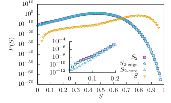
To compare the sizes of different relevant types of components, Fig. 5 shows the distributions of of the relative size of the largest connected component $S$ Hartmann2011large , the largest $2$-core $S_{\text{2-core}}$ Hartmann2017Large , the largest bi-edge-connected component $S_{\text{2-edge}}$ and the largest biconnected component $S_{2}$ for $N=500$ and $c=2$ ER graphs. Interestingly, the distributions $P(S_{2})$, $P(S_{\text{2-edge}})$ and $P(S_{\text{2-core}})$ are almost identical and only deviate in the region of very small components from each other. As would be expected by the order of Eq. 1, the probability to find very small $2$-cores is lower than to find bi-edge-connected components of the same small size, which are again slightly less probable than biconnected components of that size. Anyway, when considering ER graphs, which exhibit by construction no particular structure, the robustness properties which are determined by the biconnected component, can be with very high probability readily inferred from the 2-core.

Figure 6: Correlation histogram of our raw and biased simulational data. A large biconnected component does most probably appear in graphs whose connected component is larger than $S\gtrsim 0.6$.

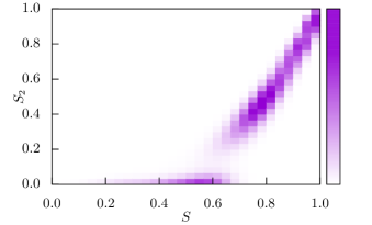
To understand the topology of the instances of very low probabilities better, we will look at the correlations of the size of the largest connected component $S$ and the largest biconnected component in Fig. 6. Note that this histogram does not reflect the probabilities, but does count the instances we generated within one of our simulations, i.e., data for many different temperatures are shown without correction for the introduced bias. Anyway, it is instructive to look at this sketch for qualitative understanding. This data is for $c=2$ ER at $N=500$. We observe that, even for our biased sampling, there are basically no large biconnected components if the connected component is smaller than $S\lesssim 0.6$. Above this point, we observe larger biconnected components, but generally very few around the size $S_{2}\approx 0.2$. Above $S\gtrsim 0.6$ the size of the largest biconnected component is strongly correlated with the size of the largest connected component.

For a qualitative understanding of this behavior, consider the following heuristic argument. For the instances without or with very small biconnected components, i.e., only short cycles, the graph is basically tree-like. Larger biconnected components are then created by connecting two nodes of the tree with each other, leading to a cycle which is on average roughly half in the order of the size of the tree, leading to the jump in the size of biconnected components. The configurations with smaller biconnected components are apparently entropically suppressed.

(a) $c=0.5$

(b) $c=1$

(c) $c=2$

Figure 7: Empirical rate function $\Phi_{N}(S_{2})$ for multiple graph sizes $N$ and connectivities $c$ of the ER graph ensemble.

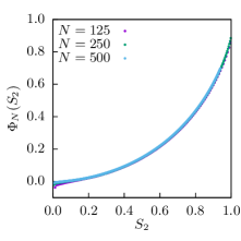
Next we will look at the empirical large deviation rate function of the measured distributions. The rate function $\Phi$ describes the behavior of distributions, whose probability density decays exponentially in the tails in respect to some parameter $N$. In this case, the parameter $N$ is the graph size. For increasing graph size $N$ the biconnected components which are not typical will be exponentially suppressed. To be more precise, the definition of the rate function $\Phi(S_{2})$ is via $P(S_{2})=\operatorname{e}^{-N\Phi(S_{2})+o(N)}$ for the large $N$ limit with the Landau symbol $o$ for terms of order less than $N$. Since we obtained the distributions over most of their support, we can access the empirical rate functions $\Phi_{N}(S_{2})=-1/N\log P(S_{2})$ for finite $N$. Note that the empirical rate functions do contain all information of the distribution. If for increasing $N$ they converge to the limiting rate function, one says the distribution follows the large deviation principle denHollander2000 ; touchette2009 .

In Fig. 7 the empirical rate functions for ER at different connectivities $c$ and for different sizes $N$ are shown. Already these comparatively small values of $N$ show remarkably similar empiric rate functions and strongly hint at a convergence to a limit form. While the rate function in the right tail for larger than typical components $S_{2}$ are already almost indistinguishable, the convergence seems a bit slower in the left tail of smaller than typical components. This behavior is very similar to the behavior of the sizes of the connected component Hartmann2011large and the $2$-core Hartmann2017Large . This means that, the large deviation principle seems to hold for this distribution.

Figure 8: Empirical rate function $\Phi_{N}(S_{2})$ for multiple graph sizes $N$ of the BA graph ensemble with $m=1.3$.

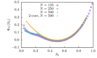
The rate function of the largest biconnected component of the BA ensemble at $m=1.3$ is shown in Fig. 8. The rate function and therefore the distribution does look qualitatively similar to the $c=2$ case of the ER ensemble (cf. Fig. 7(c)). The dip around $S_{2}\approx 0.2$ is more pronounced leading to a more severe discontinuity in the simulated finite temperature ensemble necessitating the use of Wang-Landau sampling. The main qualitative difference of the behavior of the two distributions is the behavior for very small sizes of the largest biconnected components $S_{2}$, where the empirical rate functions cross each other, hinting at some kind of finite size effect suppressing very small biconnected components in small graphs.

In comparison with the rate function of the 2-core, also shown in Fig. 8, their difference in the region of very small bicomponents respectively 2-cores, which was already observable in ER, is very strong in the BA ensemble. Despite those two observables are almost indistinguishable in the main region, they show strongly different behavior in their overall shape, i.e., the distribution of the 2-core seems convex over the region we obtained statistics for.

4 Conclusions

The biconnected component is the fundamental graph-theoretical concept which is most related to robustness properties of random networks. Nevertheless, the distribution of its size has not been studied before, to our knowledge. We used sophisticated sampling methods to obtain the distributions of the size of the largest biconnected component $S_{2}$, for multiple ER graph ensembles and a modified BA graph ensemble, over a large part of their support.

For the ER ensemble, looking into the large deviation tails of this distribution shows qualitative differences between the size of the $2$-core and the biconnected component, which are otherwise not well observable. This is even more the case for the BA ensemble where the overall shape of the distribution seems to differ. While the 2-core distribution seems convex, the distribution of the biconnected component shows a “shoulder”. These qualitative difference, however is only apparent below probabilities of $10^{-20}$ and are therefore unobservable using conventional methods.

Further, the empirical rate functions are already for the small sizes that we simulated very close to each other hinting at a very fast convergence to the limiting form. Thus, our results indicate that the large deviation principle holds for the numerically obtained distributions. This “well-behaving” of our numerical results may make it promising to address the distribution of the biconnected component by analytical means, which has not been done so far to our knowledge. Furthermore, it would be interesting to study other network ensembles, which are even more relevant for modeling robustness properties, e.g., two-dimensional networks modeling power grids dewenter2015large and other transportation networks.

5 Acknowledgments

This work was supported by the German Science Foundation (DFG) through the grant HA 3169/8-1. We also thank the GWDG (Göttingen) for providing computational resources.

6 Authors contributions

AKH conceived the study, HS wrote the first draft of the manuscript and generated most of the new data. All authors contributed ideas, simulation data and analysis to this study. All authors were involved in the preparation of the manuscript.

References

- (1) M.E.J. Newman, SIAM Review 45, 167 (2003)
- (2) S.N. Dorogovtsev, J.F.F. Mendes, Evolution of networks: from biological nets to the Internet and WWW (Oxford UNiv. Press, 2006)
- (3) M. Newman, A.L. Barabási, D. Watts, The Structure and Dynamics of Networks (Princeton University Press, 2006)
- (4) M. Newman, Networks: an Introduction (Oxford University Press, 2010)
- (5) A. Barrat, M. Barthélemy, A. Vespignani, Dynamical Processes on Complex Networks (Cambridge University Press, 2012)
- (6) M.L. Sachtjen, B.A. Carreras, V.E. Lynch, Phys. Rev. E 61, 4877 (2000)
- (7) M. Rohden, A. Sorge, M. Timme, D. Witthaut, Phys. Rev. Lett. 109, 064101 (2012)
- (8) T. Dewenter, A.K. Hartmann, New Journal of Physics 17, 015005 (2015)
- (9) R. Cohen, K. Erez, D. ben Avraham, S. Havlin, Phys. Rev. Lett. 85, 4626 (2000)
- (10) D.S. Lee, H. Rieger, EPL (Europhysics Letters) 73, 471 (2006)
- (11) C.M. Ghim, K.I. Goh, B. Kahng, Journal of Theoretical Biology 237, 401 (2005)
- (12) P. Kim, D.S. Lee, B. Kahng, Scientific Reports 5, 15567 (2015)
- (13) P. Erdős, A. Rényi, Publ. Math. Inst. Hungar. Acad. Sci. 5, 17 (1960)
- (14) D.J. Watts, S.H. Strogatz, Nature 393, 440 (1998)
- (15) A.L. Barabási, R. Albert, Science 286, 509 (1999)
- (16) R. Albert, H. Jeong, A.L. Barabási, Nature 406, 378 (2000)
- (17) D.S. Callaway, M.E.J. Newman, S.H. Strogatz, D.J. Watts, Phys. Rev. Lett. 85, 5468 (2000)
- (18) M.E.J. Newman, G. Ghoshal, Phys. Rev. Lett. 100, 138701 (2008)
- (19) C. Norrenbrock, O. Melchert, A.K. Hartmann, Phys. Rev. E 94, 062125 (2016)
- (20) P. Kim, D.S. Lee, B. Kahng, Phys. Rev. E 87, 022804 (2013)
- (21) M. Biskup, L. Chayes, S.A. Smith, Random Structures & Algorithms 31, 354 (2007)
- (22) A.K. Hartmann, The European Physical Journal B 84, 627 (2011)
- (23) A.K. Hartmann, The European Physical Journal Special Topics 226, 567 (2017)
- (24) F. den Hollander, Large Deviations (American Mathematical Society, Providence, 2000)
- (25) H. Touchette, Physics Reports 478, 1 (2009)
- (26) J. Hopcroft, R. Tarjan, Commun. ACM 16, 372 (1973)
- (27) T.H. Cormen, C.E. Leiserson, R.L. Rivest, C. Stein, Introduction to algorithms (MIT press, 2009)
- (28) B. Dezső, A. Jüttner, P. Kovács, Electronic Notes in Theoretical Computer Science 264, 23 (2011), proceedings of the Second Workshop on Generative Technologies (WGT) 2010
- (29) G. Ghoshal, Ph.D. thesis, University of Michigan (2009)
- (30) A.K. Hartmann, Phys. Rev. E 65, 056102 (2002)
- (31) S. Wolfsheimer, B. Burghardt, A.K. Hartmann, Algorithms for Molecular Biology 2, 9 (2007)
- (32) P. Fieth, A.K. Hartmann, Phys. Rev. E 94, 022127 (2016)
- (33) G. Claussen, A.K. Hartmann, S.N. Majumdar, Phys. Rev. E 91, 052104 (2015)
- (34) T. Dewenter, G. Claussen, A.K. Hartmann, S.N. Majumdar, Phys. Rev. E 94, 052120 (2016)
- (35) H. Schawe, A.K. Hartmann, S.N. Majumdar, Phys. Rev. E 97, 062159 (2018)
- (36) H. Schawe, A.K. Hartmann, arXiv preprint arXiv:1808.10698 (2018)
- (37) A.K. Hartmann, Phys. Rev. E 89, 052103 (2014)
- (38) A. Engel, R. Monasson, A.K. Hartmann, Journal of Statistical Physics 117, 387 (2004)
- (39) A.K. Hartmann, M. Mézard, Phys. Rev. E 97, 032128 (2018)
- (40) F. Wang, D.P. Landau, Phys. Rev. Lett. 86, 2050 (2001)
- (41) F. Wang, D.P. Landau, Phys. Rev. E 64, 056101 (2001)
- (42) B.J. Schulz, K. Binder, M. Müller, D.P. Landau, Phys. Rev. E 67, 067102 (2003)
- (43) R.E. Belardinelli, V.D. Pereyra, Phys. Rev. E 75, 046701 (2007)
- (44) R.E. Belardinelli, V.D. Pereyra, The Journal of Chemical Physics 127, 184105 (2007)
- (45) J. Lee, Phys. Rev. Lett. 71, 211 (1993)
- (46) R. Dickman, A.G. Cunha-Netto, Phys. Rev. E 84, 026701 (2011)
- (47) B. Efron, Ann. Statist. 7, 1 (1979)
- (48) A.P. Young, Everything You Wanted to Know About Data Analysis and Fitting but Were Afraid to Ask, SpringerBriefs in Physics (Springer International Publishing, 2015), ISBN 978-3-319-19050-1