Muon g-2 Anomaly confronted with the higgs global data in the Left-Right Twin Higgs Models

Abstract

We will examine the Left-Right Twin Higgs(LRTH) Models as a solution of muon $g-2$ anomaly with the background of the Higgs global fit data. In the calculation, the joint constrains from the theory, the precision electroweak data, the 125 GeV Higgs data, the leptonic flavor changing decay $\mu\to e\gamma$ decays, and the constraints $m_{\nu_{R}}>m_{T}>m_{W_{H}}$ are all considered. And with the small mass of the $\phi^{0}$, the direct searches from the $h\to\phi^{0}\phi^{0}$ channels can impose stringent upper limits on Br$(h\to\phi^{0}\phi^{0})$ and can reduce the allowed region of $m_{\phi^{0}}$ and $f$. It is concluded that the muon g-2 anomaly can be explained in the region of 200 GeV $\leq M\leq$ 500 GeV, 700 GeV $\leq f\leq$ 1100 GeV, 13 GeV $\leq m_{\phi^{0}}\leq$ 55 GeV, 100 GeV $\leq m_{\phi^{\pm}}\leq$ 900 GeV, and $m_{\nu_{R}}\geq$ 15 TeV after imposing all the constraints mentioned above.

I Introduction

The muon anomalous magnetic moment ($g-2$) is a very precisely measured observable, and expected to shed light on new physics . The muon $g-2$ anomaly has been a long-standing puzzle since the announcement by the E821 experiment in 2001 mug21 ; mug22 . The precision measurement of $a_{\mu}=(g-2)/2$ has been performed by the E821 experiment at Brookhaven National Laboratory BNL-g-2 , with the current world-averaged result given by WAR-g-2

$$a_{\mu}^{exp}=116592091(\pm 54)(\pm 33)\times 10^{-11},$$ (1)

Meanwhile, the Standard Model (SM) prediction from the Particle Data Group givesWAR-g-2 ,

$$a_{\mu}^{SM}=116591803(\pm 1)(\pm 42)(\pm 26)\times 10^{-11},$$ (2)

The difference between experiment and theory is

$$\Delta a_{\mu}=a_{\mu}^{exp}-a_{\mu}^{SM}=(288\pm 80)\times 10^{-11},$$ (3)

which shows a $3.6\sigma$ discrepancy, hinting at tantalizing new physics beyond the SM. It is the difference between the experimental data and the SM prediction determines the room for new physics.

There exist various new physics scenarios to explain the muon $g-2$ excess, for recent reviews, see e.g. Refs. g-2-review1 ; g-2-review2 ; g-2-review3 ; g-2-review4 ; g-2-review5 . Among these extensions, the LRTH model may also provide a explanation for the muon $g-2$ anomaly. In these models, there are six massive gauge bosons left after the symmetry breaking: the SM $Z$ and $W^{\pm}$, and extra heavier bosons, $Z_{H}$ and $W_{H}^{\pm}$. And these models also include eight scalars: one neutral pseudoscalar, $\phi^{0}$, a pair of charged scalars $\phi^{\pm}$, the SM physical Higgs $h$, and an ${\rm SU}(2)_{L}$ twin Higgs doublet $\hat{h}=(\hat{h}_{1}^{+},\hat{h}_{2}^{0})$. The lepton couplings to the pseudoscalar can be sizably enhanced by the large right-handed neutrino mass $m_{\nu_{R}}$. The pseudoscalar can give positive contributions to muon $g-2$ via the two-loop Barr-Zee diagrams.

In this work we will examine the parameter space of LRTH by considering the joint constraints from the theory, the precision electroweak data, the 125 GeV Higgs signal data, the muon $g-2$ anomaly, the lepton rare decay of $\mu\to e\gamma$, as well as the direct search limits from the LHC.

Our work is organized as follows. In Sec. II we recapitulate the LRTH models. In Sec. III we discuss the muon $g-2$ anomaly and other relevant constraints. In Sec. IV, we constrain the model using the direct search limits from the LHC, especially the Higgs global fit. Finally, the conclusion is given in Sec. VI.

II The Relevant Couplings in the LRTH Models

We need a global symmetry to implement the twin Higgs mechanism, and the global symmetry is partially gauged and spontaneously broken. At the same time, to control the quadratic divergences, we also need the twin symmetry which is identified with the left-right symmetry interchanging $L$ and $R$. The left-right symmetry implies that, for the gauge couplings $g_{2L}$ and $g_{2R}$ of $SU(2)_{L}$ and $SU(2)_{R}$, $g_{2L}=g_{2R}=g_{2}$.

In the LRTH model proposed in lrth-review ; 0611015-su ; lfv-lrth , the global symmetry is $U(4)\times U(4)$ and the gauge subgroup is $SU(2)_{L}\times SU(2)_{R}\times U(1)_{B-L}$. With the global symmetry $U(4)\times U(4)$ in the LRTH models, the Higgs field and the twin Higgs in the fundamental representation of each $U(4)$ can be written as $H$ = $(H_{L},H_{R})$ and $\hat{H}$ = $(\hat{H}_{L},\hat{H}_{R})$, respectively. After each Higgs develops a vacuum expectation value (VEV),

$$<H>^{T}=(0,0,0,f),\quad<\hat{H}>^{T}=(0,0,0,\hat{f}),$$ (4)

the global symmetry $U(4)\times U(4)$ breaks to $U(3)\times U(3)$, with the gauge group $SU(2)_{L}\times SU(2)_{R}\times U(1)_{B-L}$ down to the SM $U(1)_{Y}$.

After the Higgses obtain VEVs as shown in Eq. (4), the breaking of the $SU(2)_{R}\times U(1)_{B-L}$ to $U(1)_{Y}$ generates three massive gauge bosons, with masses proportional to $\sqrt{f^{2}+\hat{f}^{2}}$. The couplings of the these gauge bosons to the SM particles, so either precision measurements or direct searches greatly constrain their masses. The masses of the these extra gauge bosons can be large enough to avoid the constraints from the electroweak precision measurements by requiring $\hat{f}\gg f$. The problems of the large value of $\hat{f}$, however, can be eliminated by imposing certain discrete symmetry which requires that the $\hat{H}$ is odd while all the other fields are even so as to ensure the Higgs field $\hat{H}$ couples only to the gauge sector as described in ref.0611015-su .

In such models, with the global symmetry breaking from ${\rm U}(4)\times{\rm U}(4)$ to ${\rm U}(3)\times{\rm U}(3)$, and gauge symmetry from ${\rm SU}(2)_{L}\times{\rm SU}(2)_{R}\times{\rm U}(1)_{B-L}$ to ${\rm SU}(2)_{L}\times{\rm U}(1)_{Y}$ and finally to ${\rm U}(1)_{EM}$, fourteen Goldstone bosons are generated, six of which are eaten by the massive gauge bosons $Z_{H}$ and $W_{H}^{\pm}$ and the SM gauge bosons $Z^{0}$ and $W^{\pm}$, while the rest of the Goldstone bosons contain the Higgses: one neutral pseudoscalar, $\phi^{0}$, a pair of charged scalars $\phi^{\pm}$, the SM physical Higgs $h$, and an ${\rm SU}(2)_{L}$ twin Higgs doublet $\hat{h}=(\hat{h}_{1}^{+},\hat{h}_{2}^{0})$.

Since the effective Yukawa couplings suppressed by $f/\Lambda$, with $\Lambda=4\pi\hat{f}$, cannot account for the $\cal{O}(1)$ top Yukawa coupling. To give the large top quark mass, vector-like quarks are introduced. They also cancel the leading quadratic divergence of the SM gauge bosons and the top quark contributions to the Higgs masses in the loop level, except for the new heavy gauge bosons, so the hierarchy problem settles down. At the same time, the new particles such as the gauge bosons and the vector-like top singlet in the LRTH models have rich phenomenology at the LHClrth-pheno ; 0911.5567 ; lfv-lrth ; 0611015-su .

Based on the Lagrangian given in Ref. 0611015-su , we have, the couplings with fermions involved, which are concerned of our calculation in TABLE 1,

particles	vertices	particles	vertices
$W^{+}_{H\mu}\bar{t}b$	$~{}~{}e\gamma_{\mu}S_{R}P_{R}/(\sqrt{2}s_{w})$	$W^{+\mu}_{H}\bar{T}b$	$~{}~{}e\gamma_{\mu}C_{R}P_{L}/(\sqrt{2}s_{w})$
$\Phi^{+}\bar{t}b$	$-i(S_{R}m_{b}P_{L}-yS_{L}fP_{R})/f$	$\Phi^{+}\bar{T}b$	$~{}~{}i(C_{R}m_{b}P_{L}-yC_{L}fP_{R})/f$

Table 1: The three-point couplings of the charged gauge boson-fermion-fermion and those of the scalar-fermion-fermion in the LRTH models. The chirality projection operators are $P_{R,L}=(1\pm\gamma_{5})/2$.

where the mixing angles are0611015-su

$$S_{L}\sim sin\alpha_{L}\sim\frac{M}{m_{T}}sinx,~{}~{}S_{R}\sim sin\alpha_{R}\sim\frac{M}{m_{T}}(1+sin2x),~{}~{}x=\frac{v}{\sqrt{2}f}.$$ (5)

As for the parameter $M$ above, as we know, in the gauge invariant top Yukawa terms, there is the mass mixing term $M\bar{q}_{L}q_{R}$, allowed by gauge invariance. $M\neq 0$ means there is mixing between the SM-like top quark and the heavy top quark. The mixing parameter $M$ also be constrained by the $Z\to\bar{b}b$ branching ratio and oblique parameters and it usually prefers to a small value0611015-su ; 0701071 .

Neutrino oscillations oscillneutrinos imply that neutrinos are massive, and the LRTH models try to explain the origin of the neutrino masses and mass hierarchylfv-lrth . To provide lepton masses in the LRTH models, one can introduce three families doublets ${\rm SU}(2)_{L,R}$ which are charged under $SU(3)_{c}\times SU(2)_{L}\times SU(2)_{R}\times U(1)_{B-L}$ as

$$L_{L\alpha}=-i\left(\begin{array}[]{c}~{}\nu_{L\alpha}\\ l_{L\alpha}\end{array}\right):({\bf 1},{\bf 2},{\bf 1},-1),\ \ \ \ \ ~{}~{}~{}L_{R\alpha}=\left(\begin{array}[]{c}~{}\nu_{R\alpha}\\ l_{R\alpha}\end{array}\right):({\bf 1},{\bf 1},{\bf 2},-1),$$ (10)

where the family index $\alpha$ runs from 1 to 3.

Leptons can acquire masses via non-renormalisable dimension 5 operators. The charged leptons obtain their masses via the following non-renormalisable dimension $5$ operators,

$${y_{l}^{ij}\over\Lambda}(\bar{L}_{Li}H_{L})(H_{R}^{\dagger}{L}_{Rj})+{y_{\nu}^{ij}\over\Lambda}(\bar{L}_{L,i}\tau_{2}H_{L}^{*})(H_{R}^{T}\tau_{2}{L}_{Rj})+{\rm{H.c.}},$$ (11)

which will give rise to lepton Dirac mass terms $y_{\nu,l}^{ij}vf/\Lambda$, once $H_{L}$ and $H_{R}$ acquire VEVs.

The Majorana nature of the left- and right-handed neutrinos, however, makes one to induce Majorana terms ( only the mass section) in dimension 5 operators,

$${c_{L}\over\Lambda}\,\left(\overline{L}_{L\alpha}\tau_{2}H_{L}^{\dagger}\right)^{2}+{\rm H.c},\qquad{c_{R}\over\Lambda}\,\left(\overline{L}_{R\alpha}\tau_{2}H_{R}^{\dagger}\right)^{2}+{\rm H.c.}~{}.\$$ (12)

Once $H_{L}~{}(H_{R})$ obtains a VEV, both neutrino chiralities obtain Majorana masses via these operators, the smallness of the light neutrino masses, however, can not be well explained.

However, if we assume that the twin Higgs $\hat{H}_{R}$ is forbidden to couple to the quarks to prevent the heavy top quark from acquiring a large mass of order $y\hat{f}$, but it can couple to the right-handed neutrinos, one may find that lfv-lrth

$${c_{\hat{H}}\over\Lambda}\,\left(\overline{L}_{R\alpha}\tau_{2}\hat{H}_{R}^{\dagger}\right)^{2}+{\rm H.c.}~{},$$ (13)

which will give a contribution to the Majorana mass of the heavy right-handed neutrino $\nu_{R}$, in addition to those of Eq.(12).

So after the electroweak symmetry breaking, $H_{R}$ and $\hat{H}_{R}$ get VEVs, $f$ and $\hat{f}$ (Eq.(4)), respectively, we can derive the following seesaw mass matrix for the LRTH model in the basis ($\nu_{L}$,$\nu_{R}$):

$${\cal M}=\left(\begin{array}[]{cc}c{v^{2}\over 2\Lambda}&y_{\nu}{vf\over\sqrt{2}\Lambda}\\ y_{\nu}^{T}{vf\over\sqrt{2}\Lambda}&c{f^{2}\over\Lambda}+c_{\hat{H}}{\hat{f}^{2}\over\Lambda}\end{array}\right)~{}.$$ (14)

In the one-generation case there is two massive states, a heavy ($\sim\nu_{R}$) and a light one. For the case that $v<f<\hat{f}$, the masses of the two eigenstates are about $m_{\nu_{heavy}}\sim c_{\hat{H}}{\hat{f}^{2}\over\Lambda}$ and $m_{\nu_{light}}={cv^{2}\over 2\Lambda}$ lfv-lrth .

The Lagrangian in Eq.(11), (12), (13) induces neutrino masses and the mixings of different generation leptons, which may be a source of lepton flavour violating lfv-lrth . In our case we will consider the contributions to the lepton flavour violating of the charged scalars, $\phi^{\pm}$ and the heavy gauge boson, $W_{H}$. The relevant vertex interactions for these processes are explicated in the followings:

$$\phi^{-}\bar{l}\nu_{L,R}:\frac{i}{f}(m_{l_{L},\nu_{R}}P_{L}-m_{\nu_{L},l_{R}}P_{R})V_{H}\sim ic_{H}\frac{{\hat{f}}^{2}}{\Lambda f}V_{H}P_{L},$$ (15)

$$W^{-}_{L,R}\bar{l}\nu_{L,R}:\frac{e}{\sqrt{2}s_{w}}\gamma_{\mu}P_{L,R}V_{H}.$$ (16)

where $V_{H}$ is the mixing matrix of the heavy neutrino and the leptons mediated by the charged scalars and the heavy gauge bosons. The vertexes of $\phi^{-}\bar{l}\nu_{L,R}$ can also be expressed in the coupling constants. The $\phi^{-}\bar{l}\nu_{R}$, for example, is also written as $ic_{H}\frac{\hat{f}^{2}}{\Lambda f}P_{L}$ if we neglect the charged lepton masses and take $m_{\nu_{h}}=c_{H}\hat{f}^{2}/\Lambda$.

III Muon $g-2$ anomaly and relevant constraints

III.1 Numerical calculations

In this paper, the light CP-even Higgs $h$ is taken as the SM-like Higgs, $m_{h}=$ 125 GeV. Since the muon $g-2$ anomaly favors a light charged pseudoscalar with a large coupling to lepton and a heavy right-handed neutrinos, we scan over $m_{\phi}$ and $m_{\nu_{R}}$ in the following rangeslfv-lrth ; 0611015-su :

$$100~{}{\rm GeV}<m_{\phi^{\pm}}<1000~{}{\rm GeV},~{}~{}5000~{}GeV<m_{\nu_{R}}<50000~{}GeV.$$ (17)

In the following calculation, the following constraints are considered:

• From theoretical constraints and precision electroweak data, The theoretical constraints such as those from the unitarity and coupling-constant perturbativity, and the constraints from the oblique parameters $S$, $T$, $U$ will be considered1809.05857 .

• From the lepton number violating signals of the top partners0911.5567 ; lfv-lrth , we can see that right-handed neutrinos prefer to have a very large mass and the charged scalars are heavy. we can also have the constrains $m_{v_{R}}>m_{T}$ and $m_{T}>m_{W_{H}}$0911.5567 .

• The constraints from the signal data of the 125 GeV Higgs will be important, since the couplings of the 125 GeV Higgs with the SM particles in LRTH model can deviate from the SM ones and the SM-like decay modes may be modified severely. Moreover, when $m_{\phi^{0}}$ is smaller than $m_{h}/2=62.5$ GeV, the decay $h\to\phi^{0}\phi^{0}$ is kinematically allowed, and the experimental data of the 125 GeV Higgs will constrain it. We will perform $\chi^{2}_{h}$ calculation for the signal strengths of the 125 GeV Higgs, which will be discussed detailedly in Sec. IV.

• $f$ and $M$ parameter: The indirect constraints on $f$ come from the $Z$-pole precision measurements, the low energy neutral current process and the high energy precision measurements off the Z-pole: all these data prefer the parameter f to be larger than 500-600 GeV 0611015-su . On the other hand, it cannot be too large since the fine tuning is more severe for large $f$.

  In the LRTH, furthermore, the mass of the top partner $T$ is determined by the given values of $f$ and $M$. Currently, the masses of the new heavy particles, such as the $T$ have been constrained by the LHC experiments, as described in Refs. LHC-expr-1 ; LHC-expr-2 . In other words, the LHC data also imply some indirect constraints on the allowed ranges of both the parameters f and M through their correlations with $m_{T}$, as discussed in Ref. f-mt . For example, the top partner $T$ with mass below 656 GeV are excluded at $95\%$ confidence level according to the ATLAS data ATLAS-mT if one takes the assumption of a branching ratio $BR(T\to W^{+}b)=1$.

  By taking the above constraints from the electroweak precision measurements and the LHC data into account, we here assume that the values of the parameter $f$ and $M$ are in the ranges of

  $$500GeV\leq f\leq 1500GeV,\quad 0\leq M\leq 500GeV,$$ (18)

  in our numerical evaluations.

III.2 Muon $g-2$ in the LRTH models

In the LRTH, the muon $g-2$ contributions are obtained via the one-loop diagrams induced by the Higgs bosons and also from the two-loop Barr-Zee diagrams mediated by $\phi^{0}$, $h$ and $\phi^{\pm}$.

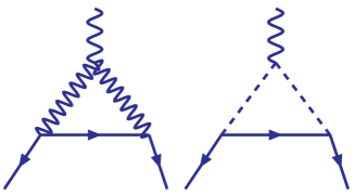
the one-loop contributions are give in the following, and the corresponding figures are given in Fig.1.

Figure 1: The one-loop contributions to $a_{\mu}$ in the LRTH models.

We can write down them one by one1loop-deltaamu :

$$\Delta a_{\mu}^{\mbox{$\scriptscriptstyle{\rm LRTH}$}}({\rm 1loop})_{W}=\frac{e^{2}}{2s_{W}^{2}}\frac{m_{\mu}^{2}}{8\pi^{2}}\int_{0}^{1}dx\frac{-6x^{3}-2x^{2}}{m_{W_{H}}^{2}x+m_{v_{R}}^{2}(1-x)},$$ (19)

$$\Delta a_{\mu}^{\mbox{$\scriptscriptstyle{\rm LRTH}$}}({\rm 1loop})_{H}=\frac{m_{\nu_{R}}^{2}}{f^{2}}\frac{m_{\mu}^{2}}{8\pi^{2}}\int_{0}^{1}dx\frac{2(x^{3}-x^{2})}{m_{H}^{2}x+m_{v_{R}}^{2}(1-x)},$$ (20)

Before we immerse into the two-loop contribution, we discuss the coupling between the boson and the scalars, and we find that they all vanish, if we parameterize the scalars in the Goldstone bosons fields as0611015-su ,

$$\begin{array}[]{ll}N~{}\to\frac{\sqrt{2}\hat{f}}{F(\cos x+2\frac{\sin x}{x})}\phi^{0},&~{}\hat{N}~{}\to-\frac{\sqrt{2}f\cos x}{3F}\phi^{0},\\ h_{1}\to 0,&~{}h_{2}\to\frac{v+h}{\sqrt{2}}-i\frac{x\hat{f}}{\sqrt{2}F(\cos x+2\frac{\sin x}{x})}\phi^{0},\\ C~{}\to-\frac{x\hat{f}}{F\sin x}\phi^{+},&~{}\hat{C}~{}\to\frac{{f\cos x}}{F}\phi^{+}.\\ \end{array}$$ (24)

where the $N,~{}\hat{N},~{}h_{1},~{}h_{2},C,~{}\hat{C}$ are in the Goldstone bosons fields,

$$H=i\frac{\sin\sqrt{\chi}}{\sqrt{\chi}}e^{i\frac{N}{2f}}\left(\begin{array}[]{c}h_{1}\\ h_{2}\\ C\\ N-if\sqrt{\chi}\cot\sqrt{\chi}\\ \end{array}\right),\ \ \hat{H}=i\frac{\sin\sqrt{\hat{\chi}}}{\sqrt{\hat{\chi}}}e^{i\frac{\hat{N}}{2\hat{f}}}\left(\begin{array}[]{c}\hat{h}_{1}\\ \hat{h}_{2}\\ \hat{C}\\ \hat{N}-i\hat{f}\sqrt{\hat{\chi}}\cot\sqrt{\hat{\chi}}\\ \end{array}\right).$$ (25)

By this parameterization, the requirement of vanishing gauge-Higgs mixing terms can be satisfied, i.e, in this redefinition of the Higgs fields, the couplings $WZ\phi^{+}$, $W\gamma\phi^{+}$, $WW\phi^{0}$, $WZ_{H}\phi^{+}$, $W\gamma_{H}\phi^{+}$, $W\phi^{0}\phi^{+}$, and $Wh\phi^{+}$ are zero, which has been verified and is quite different with those in other models such as the littlest Higgs modelsppwpi-1302.1840 .

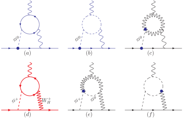
Since the coupling between the boson and the scalars $W\gamma\phi^{+}$, $Wh\phi^{+}$ and $W\phi^{0}\phi^{+}$ have been vanished, so the Barr-Zee 2-loop diagrams (e) (f) (c) in Fig. (2) disappear. Barr-Zee 2-loop diagrams (a) (b) in Fig. (2) may not be negligible even though the vertexes such as $\phi^{0}\bar{\mu}\mu$ is very small, which is proportional to the muon mass, much smaller than the masses the top and heavy top in our special case. So there are (a) (b) (d) left contributing to $a_{\mu}$.

Figure 2: The potential two-loop contributions to $a_{\mu}$ the LRTH models.

We can write down the Barr-Zee two-loop contributions of the diagram (a) (b) (d) respectivelyg-2-cal ; 1502.04199 ; 1507.07567 ,

$$\Delta a_{\mu}^{(a)}=-\frac{4m^{2}_{\mu}}{e}\frac{-e^{3}}{128\pi^{4}}\sum_{f_{j}=t,T}\frac{N_{f}^{c}Q^{2}_{f}}{m_{\mu}}\sum_{i=h,\phi^{0}}\Gamma_{\ell_{f}\ell_{i}}^{i}\Gamma_{f_{j}f_{j}}^{i}\frac{m^{f_{j}}}{m_{i}^{2}}g_{i}^{(a)}(r_{f_{j}}^{i}),$$ (26)

where $N_{f}^{c}$ and $Q_{f}$ are the number of colours and charge of fermion $f$, respectively, $\Gamma_{f_{j}f_{i}}^{i}$s are the couplings of the scalars to the fermions, and $r_{f}^{i}\equiv m_{f}^{2}/m_{\mu}^{2}$. The loop function is given by

$$g_{i}^{(a)}(r)=\int_{0}^{1}\mathrm{d}x\,\frac{N_{i}(x)}{x(1-x)-r}\ln\left(\frac{x(1-x)}{r}\right),$$ (27)

where

$$N_{h}(x)=2x(1-x)-1\,,\quad N_{\phi^{0}}(x)=-1\,.$$ (28)

$$\begin{split}\Delta a_{\mu}^{(b)}&=-\frac{4m^{2}_{\mu}}{e}\frac{e^{3}}{128\sqrt{2}\pi^{4}}\frac{v}{m_{\mu}}\quad\sum_{i=h,\phi^{0}}\frac{\Gamma_{\ell_{f}\ell_{i}}^{i}}{m_{i}^{2}}\zeta^{i}\lambda_{H^{+}H^{-}H_{i}^{0}}g_{i}^{(b)}\left(\frac{m_{H^{+}}^{2}}{m_{i}^{2}}\right),\end{split}$$ (29)

where $\zeta^{h}=-\zeta^{H}=-\zeta^{A}=1$ and the loop function is

$$g_{h,H,A}^{(b)}(r)=\int_{0}^{1}\mathrm{d}x\,\frac{x(1-x)}{x(1-x)-r}\ln\left(\frac{r}{x(1-x)}\right).$$ (30)

$$\Delta a_{\mu}^{(d)}({ttb+bbt}) = -\frac{4m^{2}_{\mu}}{e}\frac{-e^{3}S_{R}V_{H}}{1024\pi^{4}sin^{2}\theta_{w}}\frac{N_{t}^{c}V_{tb}^{*}}{m_{\phi}^{2}-m_{W_{H}}^{2}}$$

$$\int_{0}^{1}dx[Q_{t}x+Q_{b}(1-x)]\left[G\left(\frac{m_{t}^{2}}{m_{H^{+}}^{2}},\frac{m_{b}^{2}}{m_{H^{+}}^{2}}\right)-G\left(\frac{m_{t}^{2}}{m_{W}^{2}},\frac{m_{b}^{2}}{m_{W}^{2}}\right)\right]$$

$$\times\left[\left({\Gamma_{tb}^{\phi^{+},L}}^{*}{\Gamma_{\nu_{f}\mu}^{\phi^{+}}}\right)\frac{m_{b}}{m_{\mu}}x(1-x)-\left({\Gamma_{tb}^{\phi^{+},R}}^{*}{\Gamma_{\nu_{f}\mu}^{\phi^{+}}}\right)\frac{m_{t}}{m_{\mu}}x(1+x)\right]$$

$$\Delta a_{\mu}^{(d)}({TTb+bbT}) = -\frac{4m^{2}_{\mu}}{e}\frac{-e^{3}C_{R}V_{H}}{1024\pi^{4}sin^{2}\theta_{w}}\frac{1}{m_{\phi}^{2}-m_{W_{H}}^{2}}$$

$$\int_{0}^{1}dx[Q_{T}x+Q_{b}(1-x)]\left[G\left(\frac{m_{T}^{2}}{m_{H^{+}}^{2}},\frac{m_{b}^{2}}{m_{H^{+}}^{2}}\right)-G\left(\frac{m_{T}^{2}}{m_{W}^{2}},\frac{m_{b}^{2}}{m_{W}^{2}}\right)\right]$$

$$\times\left[\left({\Gamma_{Tb}^{\phi^{+},R}}^{*}{\Gamma_{\nu_{f}\mu}^{\phi^{+}}}\right)\frac{m_{b}}{m_{\mu}}x(1-x)-\left({\Gamma_{Tb}^{\phi^{+},L}}^{*}{\Gamma_{\nu_{f}\mu}^{\phi^{+}}}\right)\frac{m_{T}}{m_{\mu}}x(1+x)\right]$$

where the loop function is defined as,

$$G(r^{a},r^{b})=\frac{\ln\left(\frac{r^{a}x+r^{b}(1-x)}{x(1-x)}\right)}{x(1-x)-r^{a}x-r^{b}(1-x)}\,,$$ (33)

and $\Gamma_{tb}^{\phi^{+},R}$ and $\Gamma_{tb}^{\phi^{+},L}$ are the right-handed and left-handed couplings of the vertex $\phi^{+}\bar{t}b$, which are given in Table 1. From Table 1, we also see that the top vector-like partner $T$ enter into the triangle loop just as the top quark, and the contribution to $a_{\mu}$ is

$$\Delta a_{\mu}^{TTb}({\rm 2loop-BZ})=\Delta a_{\mu}^{ttb}({\rm 2loop-BZ})(m_{t}\to m_{T},~{}N_{t}^{c}\to N_{T}^{c})$$ (34)

where for the vector-like fermion, $N_{T}^{c}=1$.

By the way, we should note that in the Barr-Zee 2-loop diagrams there are no two scalars or two $W^{\pm}$ charged bosons connect to the triangle loop simultaneously, which is induced by the helicity constraints since between the two charged particles, the fermion is the bottom qurak, which mass is much smaller than that of the top quark, and the slash momentum terms must vanish undergoing a single $\gamma$ matrix. Of course, the discussion here is very crudely, and explicit and detailed discussion can be found in Ref. 1502.04199 .

As the enhancement factor $m^{2}_{f}/m^{2}_{\mu}$ could easily overcome the loop suppression phase space factor $\alpha/\pi$, the two-loop contributions can be larger than one-loop ones. In the LRTH, since the CP-odd Higgs coupling to the lepton is proportional to $m_{v_{R}}$, the LRTH can sizably enhance the muon g-2 for a light CP-odd scalar and a large right-handed neutrino mass $m_{v_{R}}$.

IV Global fit of the 125 GeV Higgs

The 125 GeV Higgs signal data include a large number of observales and we will perform a global fit to the 125 GeV Higgs signal data. For the given neutral SM-like scalar-field $h$ and its couplings, the $\chi^{2}_{h}$ function can be defined as

$$\chi^{2}_{h}\;=\;\sum_{k}\;\frac{\left(\mu_{k}-\hat{\mu}_{k}\right)^{2}}{\sigma_{k}^{2}}\,,$$ (35)

where $k$ runs over the different production(decay) channels considered, and $\hat{\mu}_{k}$ and $\sigma_{k}$ denote the measured Higgs signal strengths and their one-sigma errors, respectively. $\mu_{k}$ is the corresponding theoretical predictions for the LRTH parameters, as given later in Eqs. (42) and (49).

IV.1 Relevant Lagrangian and the Couplings

After diagonaling, the Yukawa lagrangians can be written as,

$$\mathcal{L}_{Y}=-\sum_{f=d,l}y_{f}h\bar{f}P_{R}f-\sum_{f=t,T}y_{f}h\bar{u}P_{L}u$$ (36)

From Eq.(36) and the couplings in Ref. 0611015-su , we can get the interactions between the Higgs boson and the pairs of $\bar{b}b,~{}\bar{l}l,~{}t\bar{t},~{}T\overline{T},~{}VV(V=W,W_{H}),\phi^{+}\phi^{-}$:

$$y_{b}=-\frac{m_{b}}{v}C_{L}C_{R}=-\frac{m_{b}}{v}\rho_{b},~{}y_{l}=-\frac{m_{l}}{v}C_{L}C_{R}=-\frac{m_{l}}{v}\rho_{l},$$ (37)

$$~{}y_{t}=-\frac{m_{t}}{v}C_{L}C_{R}=-\frac{m_{t}}{v}\rho_{t},~{}y_{T}=y(S_{R}S_{L}-C_{L}C_{R}x)/\sqrt{2},$$ (38)

$$h~{}W^{+}_{\mu}~{}W^{-}_{\nu}:~{}~{}em_{W}/s_{W}=\rho_{W}m_{W}^{2}/v,~{}~{}\rho_{W}=ev/(m_{w}s_{W})$$ (39)

$$h~{}W_{H\mu}^{+}~{}W_{H\nu}^{-}:-e^{2}f~{}x~{}g_{\mu\nu}/(\sqrt{2}s_{w}^{2})=y_{W_{H}}g_{\mu\nu},$$ (40)

$$h\phi^{+}\phi^{-}:y_{\phi},~{}y_{\phi}=-x\frac{2m_{h}^{2}-2m_{\phi}^{2}}{3\sqrt{2}f}.$$ (41)

$\rho_{t}=\rho_{b}=\rho_{\tau}=C_{L}C_{R},~{}\rho_{W}=\frac{e*v}{m_{W}S_{W}}$ are the ratios of $hff,~{}hWW$ vertexes in LRTH and the standard models.

IV.2 Higgs Signal Strengths

The so-called signal strengths, which are employed in the experimental data on Higgs searches, measuring the observable cross sections in ratio to the corresponding SM predictions. At the LHC, the SM-like Higgs particle is generated by the following relevant production mechanisms: gluon fusion ($gg\rightarrow H$), vector boson fusion ($qq^{\prime}\rightarrow qq^{\prime}VV\rightarrow qq^{\prime}H$), associated production with a vector boson ($q\bar{q}^{\prime}\rightarrow WH/ZH$), and the associated production with a $t\bar{t}$ pair ($q\bar{q}/gg\rightarrow t\bar{t}H$). The Higgs decay channels are $\gamma\gamma$, $ZZ^{(*)}$, $WW^{(*)}$, $b\bar{b}$ and $\tau^{+}\tau^{-}$.

In order to fit the experimental measurements, we can write down the following ratios:

$$\mu_{gg\gamma\gamma} \equiv\frac{\sigma(pp\to h)\,\text{Br}(h\to\gamma\gamma)}{\sigma(pp\to H)_{\mathrm{SM}}\,\text{Br}(H\to\gamma\gamma)_{\mathrm{SM}}}\,,\qquad \mu_{t\bar{t}h\gamma\gamma} \equiv\frac{\sigma(pp\to t\bar{t}h)\,\text{Br}(h\to\gamma\gamma)}{\sigma(pp\to t\bar{t}H)_{\mathrm{SM}}\,\text{Br}(H\to\gamma\gamma)_{\mathrm{SM}}}\,,$$

$$\mu_{ggVV} \equiv\frac{\sigma(pp\to h)\,\text{Br}(h\to VV)}{\sigma(pp\to H)_{\mathrm{SM}}\,\text{Br}(H\to VV)_{\mathrm{SM}}}\,, \mu_{t\bar{t}hVV} \equiv\frac{\sigma(pp\to t\bar{t}h)\,\text{Br}(h\to VV)}{\sigma(pp\to t\bar{t}H)_{\mathrm{SM}}\,\text{Br}(H\to VV)_{\mathrm{SM}}}\,,$$

$$\mu_{ggff} \equiv\frac{\sigma(pp\to h)\,\text{Br}(h\to ff)}{\sigma(pp\to H)_{\mathrm{SM}}\,\text{Br}(H\to ff)_{\mathrm{SM}}}\,, \mu_{t\bar{t}hff} \equiv\frac{\sigma(pp\to t\bar{t}h)\,\text{Br}(h\to ff)}{\sigma(pp\to t\bar{t}H)_{\mathrm{SM}}\,\text{Br}(H\to ff)_{\mathrm{SM}}}\,,$$

$$\mu_{Vh\gamma\gamma} \equiv\frac{\sigma(pp\to Vh)\,\text{Br}(h\to\gamma\gamma)}{\sigma(pp\to VH)_{\mathrm{SM}}\,\text{Br}(H\to\gamma\gamma)_{\mathrm{SM}}}\,,\qquad \mu_{VBF\gamma\gamma} \equiv\frac{\sigma(pp\to qqh)\,\text{Br}(h\to\gamma\gamma)}{\sigma(pp\to qqH)_{\mathrm{SM}}\,\text{Br}(H\to\gamma\gamma)_{\mathrm{SM}}}\,,$$

$$\mu_{VhVV} \equiv\frac{\sigma(pp\to Vh)\,\text{Br}(h\to VV)}{\sigma(pp\to H)_{\mathrm{SM}}\,\text{Br}(H\to VV)_{\mathrm{SM}}}\,, \mu_{VBFVV} \equiv\frac{\sigma(pp\to qqh)\,\text{Br}(h\to VV)}{\sigma(pp\to qqH)_{\mathrm{SM}}\,\text{Br}(H\to VV)_{\mathrm{SM}}}\,,$$

$$\mu_{Vhff} \equiv\frac{\sigma(pp\to Vh)\,\text{Br}(h\to ff)}{\sigma(pp\to H)_{\mathrm{SM}}\,\text{Br}(H\to ff)_{\mathrm{SM}}}\,, \mu_{VBFff} \equiv\frac{\sigma(pp\to qqh)\,\text{Br}(h\to ff)}{\sigma(pp\to qqH)_{\mathrm{SM}}\,\text{Br}(H\to ff)_{\mathrm{SM}}}\,,$$ (42)

where $V={W,\!\ Z}$.

The ratio of the branching fraction will be expressed as:

$$\frac{\text{Br}(h\to X)}{\text{Br}(H\to X)_{\mathrm{SM}}}\;=\;\dfrac{1}{\rho(h)}\;\frac{\Gamma(h\to X)}{\Gamma(H\to X)_{\mathrm{SM}}}\;\,,$$ (43)

where $\rho(h)$ is the total decay width of the scalar $h$ in units of the SM Higgs width,

$$\rho(h) = \frac{\Gamma(h)}{\Gamma_{\mathrm{SM}}(H)}$$ (45)

$$= \frac{\Gamma^{BSM}(h)+\Gamma(h\to\varphi^{0}\varphi^{0})}{\Gamma_{\mathrm{SM}}(H)}$$ (46)

$$= \frac{\Gamma^{BSM}(h)}{\Gamma_{\mathrm{SM}}(H)}+\frac{\Gamma(h\to\varphi^{0}\varphi^{0})}{\Gamma_{\mathrm{SM}}(H)},$$ (47)

where the existence of the $h\to\varphi^{0}\varphi^{0}$ means in the LRTH models when $\varphi^{0}$ mass is less than $m_{h}/2$, the channel $h\to\varphi^{0}\varphi^{0}$ will be open, and the total width of $h$ should changed into $\Gamma^{LRTH}(h)+\Gamma(h\to\varphi^{0}\varphi^{0})$, where $\Gamma^{LRTH}(h)$ is corresponding to SM channels. $\Gamma(h\to\varphi^{0}\varphi^{0})$ can be written as

$$\Gamma(h\to\varphi^{0}\varphi^{0})=\frac{g^{2}_{h\varphi^{0}\varphi^{0}}}{8\pi m_{h}}\sqrt{1-\frac{4m^{2}_{\varphi}}{m_{h}^{2}}}$$ (48)

where $g_{h\varphi^{0}\varphi^{0}}=\frac{vm_{h}^{2}}{54f^{2}}[11+15(1-\frac{2m_{\varphi}^{2}}{m_{h}^{2}})]$1312.4004 .

Particularizing to the LRTH and assuming only one dominant production channel in each case, we have:

$$\mu_{gg\gamma\gamma}=C_{gg}C_{\gamma\gamma}\rho(h)^{-1},~{}~{}\mu_{ggVV}=C_{gg}\rho_{W}^{2}\rho(h)^{-1},~{}~{}\mu_{ggff}=C_{gg}\rho_{f}^{2}\rho(h)^{-1},$$

$$\mu_{t\bar{t}h\gamma\gamma}=\rho_{t}^{2}C_{\gamma\gamma}\rho(h)^{-1},~{}~{}\mu_{t\bar{t}hVV}=\rho_{t}^{2}\rho_{W}^{2}\rho(h)^{-1},~{}~{}\mu_{t\bar{t}hff}=\rho_{t}^{2}\rho_{f}\rho(h)^{-1},$$

$$\mu_{VBF\gamma\gamma}=\rho_{W}^{2}C_{\gamma\gamma}\rho(h)^{-1},~{}~{}\mu_{VBFVV}=\rho_{W}^{2}\rho_{W}^{2}\rho(h)^{-1},~{}~{}\mu_{VBFff}=\rho_{W}^{2}\rho_{f}^{2}\rho(h)^{-1},$$

$$\mu_{Vh\gamma\gamma}=\rho_{W}^{2}C_{\gamma\gamma}\rho(h)^{-1},~{}~{}\mu_{VhVV}=\rho_{W}^{2}\rho_{W}^{2}\rho(h)^{-1},~{}~{}\mu_{Vhff}=\rho_{W}^{2}\rho_{f}\rho(h)^{-1}$$ (49)

Note that $\rho_{W}=\rho_{Z}$.

The one-loop functions are given by

$$C_{gg}=\frac{\sigma(gg\to h)}{\sigma(gg\to h)_{\mathrm{SM}}}=\frac{|\sum_{q=t,T}y_{q}\mathcal{F}(x_{q})|^{2}}{|\sum_{q=t}y_{t}\mathcal{F}(x_{q})|^{2}}$$ (50)

where $y_{t}=y_{t}v/\sqrt{2}$, and

$$C_{\gamma\gamma}\; =\;\frac{\Gamma(h\to\gamma\gamma)}{\Gamma(h\to\gamma\gamma)_{\mathrm{SM}}}$$ (51)

$$=\;\frac{\Big{|}\sum_{f}y_{f}N_{C}^{f}Q_{f}^{2}\mathcal{F}(x_{f})+\mathcal{F}_{1}(x_{W})y_{W}+\mathcal{F}_{1}(x_{W_{H}})y_{W_{H}}+\mathcal{F}_{0}(x_{\phi^{\pm}})y_{\phi}\Big{|}^{2}}{\Big{|}\sum_{f}N_{C}^{f}Q_{f}^{2}\mathcal{F}(x_{f})+\mathcal{G}(x_{W})\Big{|}^{2}}\qquad$$

with $N_{C}^{f}$ and $Q_{f}$ the number of colours and the electric charge of the fermion $f$, and $x_{f}=4m_{f}^{2}/M_{h}^{2}$, $x_{W}=4M_{W}^{2}/M_{h}^{2}$ and $x_{\phi^{\pm}}=4M_{\phi^{\pm}}^{2}/M_{h}^{2}$. Note that the ratios (42) are defined for $M_{h}=M_{h_{\mathrm{SM}}}$. The functions $\mathcal{F}(x_{f})$ and $\mathcal{F}_{1}(x_{W})$ contain the contributions of the triangular 1-loop from fermions and $W^{\pm}$ bosons. The masses of the first two fermion generations will be neglected. Since $\mathcal{F}(x_{f})$ vanishes for massless fermions, we only need to consider the top and the vector-like top contributions, which correspond large Yukawa couplings.

The explicit expressions of the different loop functions can be given as:

$$\mathcal{F}(x)\; =\;\frac{x}{2}[4+(x-1)f(x)]\,,\qquad \mathcal{F}_{1}(x)\; =\;-2-3x+\Big{(}\frac{3}{2}x-\frac{3}{4}x^{2}\Big{)}f(x)\,,$$

$$\mathcal{F}_{0}(x)\; =\;-x-\frac{x^{2}}{4}f(x)\,, \mathcal{K}(x)\; =\;-\frac{x}{2}f(x)\,,$$ (52)

with

$$f(x)\;=\;\begin{cases}-4\arcsin^{2}(1/\sqrt{x})\,,\quad&x\geqslant 1\\[3.0pt] \Big{[}\ln\Big{(}\frac{1+\sqrt{1-x}}{1-\sqrt{1-x}}\Big{)}-i\pi\Big{]}^{2}\,,&x<1\end{cases}\,.$$ (53)

V Results and discussions

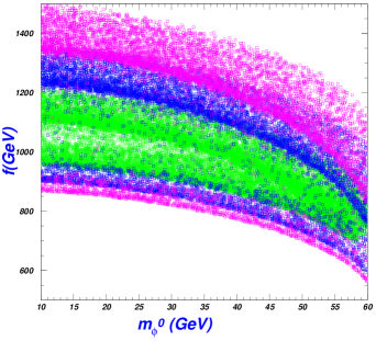
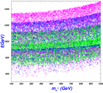
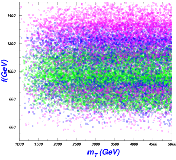
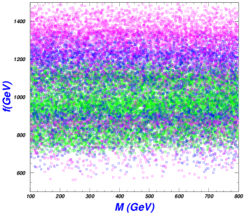
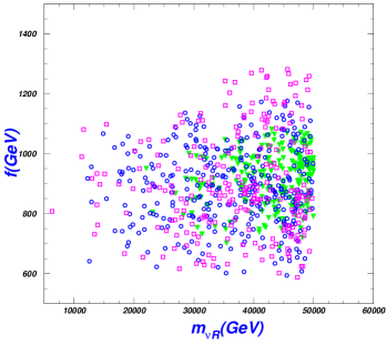
Figure 3: The surviving samples within 1$\sigma$, 2$\sigma$, and 3$\sigma$ ranges of $\chi^{2}_{h}$ on the planes of $f$ versus $m_{\phi^{0}}$, $m_{\phi^{\pm}}$, $m_{T}$, and $M$. The green, blue and the pink points are respectively within the $1\sigma$,$2\sigma$, and $3\sigma$ regions of $\chi^{2}_{h}$.

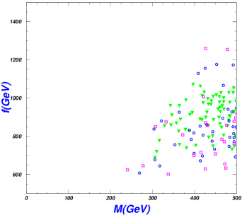
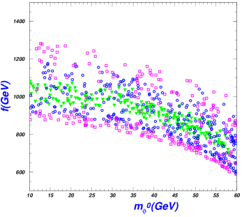
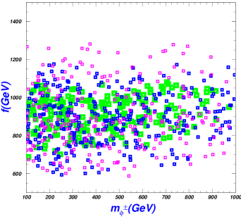
Figure 4: The samples satisfying the constraints of Higgs global fit within 1$\sigma$, 2$\sigma$, and 3$\sigma$ ranges, on the planes of $f$ versus $M$, $m_{\phi^{0}}$, $m_{\phi^{\pm}}$, and $m_{\nu_{R}}$, with the constraints of the $a_{\mu}$ from the experiemnts. All the samples are allowed by the constraints of muon $g-2$. The green, blue and the pink points are respectively within the $1\sigma$,$2\sigma$, and $3\sigma$ regions of $\chi^{2}_{h}$.

In Fig. 3, we project the surviving samples within 1$\sigma$, 2$\sigma$, and 3$\sigma$ ranges of $\chi^{2}_{h}$ on the planes of $f$ versus $m_{\phi^{0}}$, $m_{\phi^{\pm}}$, $m_{T}$, and $M$, the exclusion limits from searches for Higgs at LEP, the signal data of the 125 GeV Higgs, and the flavor changing constraints of $\mu\to e\gamma$lfv-lrth . Fig. 3 shows that the of $\chi^{2}_{h}$ value favors a little large $f$. We can see from the upper panel that if the value of $f$ is small, the value of $\chi^{2}_{h}$ prefer to have a large $m_{\phi^{0}}$ and a small $m_{\phi^{\pm}}$. From the lower-left panel of Fig. 3 that the value of $\chi^{2}_{h}$ is favored to a large top partner mass $m_{T}$.

In Fig. 4, we project the surviving samples within 1$\sigma$, 2$\sigma$, and 3$\sigma$ on the planes of $f$ versus $m_{\phi^{0}}$, $m_{\phi^{\pm}}$, $m_{T}$, and $M$ after imposing the constraints from the muon g-2 anomaly, the lepton flavor changing decay. The lower-left panel shows that the surviving data preferring to a large mixing parameter $M$, about $200-500$ GeV.

Fig. 4 shows that with the limits from muon $g-2$, the Higgs global fit and the lepton decay $\mu\to e\gamma$ being satisfied, the muon $g-2$ anomaly can be explained in the regions of 200 GeV $\leq M\leq$ 500 GeV, 700 GeV $\leq f\leq$ 1100 GeV, 10 GeV $\leq m_{\phi^{0}}\leq$ 60 GeV, 100 GeV $\leq m_{\phi^{\pm}}\leq$ 900 GeV, and $m_{\nu_{R}}\geq$ 15 TeV. Fig. 4 shows that in the range of 10 GeV $\leq m_{\phi^{0}}\leq$ 60 GeV and a light $f$ constrained by the decay $\mu\to e\gamma$, the muon $g-2$ anomaly can be explained for a large enough $m_{\nu_{R}}$, which constraint severely the models which introduce extra right-handed neutrinos to give the natural light neutrino masses. Since the contributions of $m_{\nu_{R}}$ to the muon $g-2$ anomaly have destructive interference with the prediction, there may not exist many samples, and the model survives in narrow space, as shown in the lower-right panel of Fig. 4.

VI Conclusion

The muon $g-2$ anomaly can be explained in the LRTH model. After imposing various relevant theoretical and experimental constraints, we performed a scan over the parameter space of this model to identify the ranges in favor of the muon $g-2$ explanation, and the Higgs direct search limits from LHC constraint strongly. We find that the muon g-2 anomaly can be accommodated in the region of 300 GeV $\leq M\leq$ 500 GeV, 700 GeV $\leq f\leq$ 1100 GeV, 10 GeV $\leq m_{\phi^{0}}\leq$ 60 GeV, 100 GeV $\leq m_{\phi^{\pm}}\leq$ 900 GeV, and $m_{\nu_{R}}\geq$ 15 TeV, after imposing the joint constraints from the theory, the precision electroweak data, the 125 GeV Higgs signal data, and the leptonic decay.

References

• (1) H. N. Brown et al. [Muon g-2 Collaboration], Phys. Rev. Lett. 86, (2001) 2227, hep-ex/0102017.
• (2) G. W. Bennett et al. [Muon g-2 Collaboration], Phys. Rev. D 73, (2006) 072003, hep-ex/0602035.
• (3) G. W. Bennett et al. (Muon g-2), Phys. Rev. D73, 072003 (2006), arXiv:hep-ex/0602035.
• (4) C. Patrignani et al. (Particle Data Group), Chin. Phys. C40, 100001 (2016).
• (5) J. P. Miller, E. de Rafael, and B. L. Roberts, Rept. Prog. Phys. 70, 795 (2007), arXiv:hep-ph/0703049.
• (6) F. Jegerlehner and A. Nyffeler, Phys. Rept. 477, 1 (2009), arXiv:0902.3360.
• (7) J. P. Miller, E. de Rafael, B. L. Roberts, and D. St ockinger, Ann. Rev. Nucl. Part. Sci. 62, 237 (2012).
• (8) M. Lindner, M. Platscher, and F. S. Queiroz, Phys. Rept. 731, 1 (2018), arXiv:1610.06587.
• (9) F. Jegerlehner, Springer Tracts Mod. Phys. 274, pp.1 (2017).
• (10) Z. Chacko, H.-S. Goh, R. Harnik, Phys. Rev. Lett. 96, 231802(2006), arXiv:hep-ph/0506256; Z. Chacko, Y. Nomura, M. Papucci, and G. Perez, JHEP  0601, (2006)126, arXiv:hep-ph/0510273; Z. Chacko, H. Goh, R. Harnik, JHEP  0601, (2006) 108, arXiv:hep-ph/0512088; J. C. Pati and A. Salam, Phys. Rev. D 10, 275 (1974); R. N. Mohapatra and J. C. Pati, Phys. Rev. D 11, (1975)566; R. N. Mohapatra and J. C. Pati, Phys. Rev. D 11, (1975)2558; H. S. Goh and C. Krenke, Phys. Rev. D 76, (2007) 115018, arXiv:0707.3650.
• (11) Hock-Seng Goh, Shufang Su, Phys. Rev. D 75, (2007)075010, arXiv:hep-ph/0611015.
• (12) Asmaa Abada and Irene Hidalgo, Phys. Rev. D 77, (2008) 113013, arXiv:hep-ph/0711.1238; Guo-Li Liu, Fei Wang, Kuan Xie, Xiao-Fei Guo, Phys. Rev. D 96, (2017) 035005, arXiv:1701.00947.
• (13) Hock-Seng Goh, Christopher A. Krenke, Phys. Rev. D 81, (2010) 055008, arXiv:0911.5567.
• (14) See for examples, Yao-Bei Liu, Zhen-Jun Xiao, J. Phys. G 42,(2015) 065005, arXiv:1412.5905; Chong-Xing Yue, Hui-Di Yang, Wei Ma, Nucl. Phys. B 818, (2009) 1, arXiv:0903.3720. Lei Wang, Jin Min Yang, JHEP  1005:024,2010, arXiv:1003.4492. Guo Zhan-Ying, Yang Guang, Yang Bing-Fang, Chin.Phys. C37, (2013) 103101, arXiv:1304.2249. Yao-Bei Liu, Zhen-Jun Xiao, Nucl.Phys. B892 (2015) 63, arXiv:1409.6050. Ethan M. Dolle, Shufang Su, Phys. Rev. D 77, (2008) 075013, arXiv:0712.1234.
• (15) J.-Y. Lee, D.-W Jung, J.Korean Phys.Soc. 63 (2013) 1114, hep-ph/0701071.
• (16) See, for example, M. C. Gonzalez-Garcia and Y. Nir, Rev. Mod. Phys. 75, 345(2003); V. Barger, D. Marfatia, and K. Whisnant, Int. J. Mod. Phys E12, 569(2003); A. Y. Smimov, arXiv: hep-ph/0402264; M. C. Gonzalez-Garcia and M. Maltoni, Physics Reports 460, 1(2007), arXiv:0704.1800.
• (17) Lei Wang, Jin Min Yang, Mengchao Zhang, Yang Zhang, Phys. Lett. B 788, (2019) 519, arXiv:1809.05857.
• (18) G. Aad et al. (ATLAS Collaboration), JHEP 1211 (2012) 094; Phys.Lett. B 712, 22 (2012); Phys.Rev. D 86, 012007 (2012); S. Chatrchyan et al. (CMS Collaboration), JHEP 1301 (2013) 154. Phys.Lett. B 718, 307 (2012).
• (19) T. Aaltonen et al., (CDF Collabration), Phys.Rev.Lett. 102 (2009) 031801; V.M. Abazov et al., (D0 Collaboration), Phys.Lett. B 695 (2011) 88; J. Beringer et al., (Particle Data Group collaboration), Phys.Rev. D 86 (2012) 010001; S. Chatrchyan et al., (CMS Collaboration), Phys.Lett. B 720 (2013) 63.
• (20) Y.-B. Liu, S. Cheng and Z.-J. Xiao, Phys.Rev. D 89 (2014) 015013.
• (21) G. Aad et al. (ATLAS Collaboration), Phys.Lett. B 718 (2013) 1284.
• (22) J. P. Leveille, Nucl. Phys. B 137, 63 (1978); S. R. Moore, K. Whisnant, and Bing-Lin Young, Phys. Rev. D 31, (1985) 105; Farinaldo S. Queiroz, William Shepherd, Phys. Rev. D 89 (2014) 095024, arXiv:1403.2309.
• (23) Guo-Li Liu, Fei Wang, Shuo Yang, Phys. Rev. D 88, (2013) 115006, arXiv:1302.1840.
• (24) A. Broggio, E. J. Chun, M. Passera, K. M. Patel and S. K. Vempati, JHEP 1411 (2014) 058, [arXiv:1409.3199 [hep-ph]]; L. Wang and X. F. Han, JHEP05, 039 (2015), arXiv:1412.4874 [hep-ph]; A. Dedes and H. E. Haber, JHEP 0105 (2001) 006 [hep-ph/0102297]; J. F. Gunion, JHEP 0908 (2009) 032 [arXiv:0808.2509 [hep-ph]]; K. M. Cheung, C. H. Chou and O. C. W. Kong, Phys. Rev. D 64 (2001) 111301 [hep-ph/0103183]; D. Chang, W. F. Chang, C. H. Chou and W. Y. Keung, Phys. Rev. D 63 (2001) 091301 [hepph/0009292]; M. Krawczyk, Acta Phys. Polon. B 33 (2002) 2621 [hep-ph/0208076]; F. Larios, G. Tavares-Velasco and C. P. Yuan, Phys. Rev. D 64 (2001) 055004 [hep-ph/0103292]; K. Cheung and O. C. W. Kong, Phys. Rev. D 68 (2003) 053003 [hep-ph/0302111]; A. Arhrib and S. Baek, Phys. Rev. D 65 (2002) 075002 [hep-ph/0104225]; S. Heinemeyer, D. Stockinger and G. Weiglein, Nucl. Phys. B 690 (2004) 62 [hep-ph/0312264]; O. C. W. Kong, hep-ph/0402010; K. Cheung, O. C. W. Kong and J. S. Lee, JHEP 0906 (2009) 020 [arXiv:0904.4352 [hep-ph]].
• (25) Victor Ilisie, JHEP  04, (2015) 077, arXiv:1502.04199 [hep-ph].
• (26) Andreas Crivellin, Julian Heeck, Peter Stoffer, Phys. Rev. Lett. 116,(2016) 081801, arXiv:1507.07567.
• (27) Yao-Bei Liu, Zhen-Jun Xiao, JHEP  1402 (2014) 128, arXiv:1312.4004.