Learning Representations of Missing Data for
Predicting Patient Outcomes

Abstract

Extracting actionable insight from Electronic Health Records (EHRs) poses several challenges for traditional machine learning approaches. Patients are often missing data relative to each other; the data comes in a variety of modalities, such as multivariate time series, free text, and categorical demographic information; important relationships among patients can be difficult to detect; and many others. In this work, we propose a novel approach to address these first three challenges using a representation learning scheme based on message passing. We show that our proposed approach is competitive with or outperforms the state of the art for predicting in-hospital mortality (binary classification), the length of hospital visits (regression) and the discharge destination (multiclass classification).

1 Introduction

Healthcare is an integral service in modern societies. Improving its quality and efficiency has proven to be difficult and costly. Electronic health records (EHRs) provide a wealth of information carrying the potential to improve treatment quality and patient outcomes. Extracting useful and actionable medical insights from EHRs, however, poses several challenges both to traditional statistical and machine learning techniques.

First, not all patients receive the same set of laboratory tests, examinations, consultations, etc., while they are at the hospital. Thus, many patients have missing and incomplete data, relative to other patients. Second, the various medical conditions and the corresponding treatment activities yield different kinds of data. For example, a blood oxygen saturation sensor may collect numeric values for a given amount of time at fixed frequency, while a consultation with a physician may produce only free text notes of the physician’s interpretation. That is, there are multiple modalities (or attribute types) of data, and these modalities have variations due to a number of external factors. Third, patients may share important relationships which are not easily captured in typical data representations. For example, family members often share a similar genetic background. Likewise, patients with similar initial diagnoses may share underlying characteristics which are difficult to capture in traditional models. Thus, it is important to explicitly model relationships among patients that capture some form of disease or treatment affinity.

Recent work on representation learning for graph-structured data has specifically addressed the last two problems albeit in different domains. In that line of work, edges in an affinity graph connect instances deemed similar in some way, and a message passing scheme is used to learn representations of the data modalities associated with each instance. While several message-passing approaches to graph representation learning have been proposed (?; ?; ?), we base our work on embedding propagation (Ep), a method that is both unsupervised and learns a representation specific to each data modality (?).

Ep has several characteristics that make it well-suited for the problem of learning from medical records. First, it provides a method for learning and combining representations, or embeddings, of the various data modalities typically found in EHRs. For instance, it is possible to simultaneously learn embeddings of free-text notes and to combine these with embeddings learned for sensor time series data. Second, as we will propose in this work, due to its unsupervised reconstruction loss, Ep allows us to learn a vector representation for every data modality and every patient, even if that particular data modality is not observed at all for some of the patients. Third, Ep learns representations for each data modality independently; thus, it is possible to distinguish between the influence of these independently learned modality representations on the predictions.

Intuitively, embedding propagation learns data representations such that representations of nodes close in the graph, that is, nodes similar in one or several ways, are more similar to each other than those of nodes far away in the graph. The representations can then be used in traditional downstream machine learning tasks. In the context of EHRs, patients are modeled as nodes in the graph, and similarity relationships between patients are modeled with edges.

In this work, we extend the embedding propagation framework to account for missing data. In particular, for each data modality, we learn two representations for each patient; the first representation carries information about the observed data, while the second representation is learned to account for missing data. Learning an explicit representation of missing data within the graph-based learning framework has the advantage of propagating representations of missing data throughout the graph such that these representations are also informed by representations of neighboring patients. Combining these learned feature representations gives a complete representation for downstream tasks.

We use a recently-introduced benchmark based on the MIMIC-III dataset (?) to evaluate the proposed approach and show that it is competitive with the state of the art when using a single data modality, numeric time series observations. After augmenting the data with additional data modalities, including free text from physicians’ notes and demographic information, we outperform the state of the art on two of the three tasks we consider in this work, namely, length of hospital stay and discharge destination prediction.

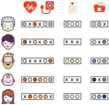
(a)

(b)

Figure 1: (a) Illustration of patients and the corresponding time-series, text, and demographic data. Missing data is indicated with an $\mathtt{x}$. (b) A patient affinity graph constructed with a subset of the patient attributes. The graph structure is leveraged in the EP framework.

The rest of this paper is structured as follows. In Section 2, we describe the data that we use in this work. Section 3 introduces Ep and describes our novel contribution for handling missingness within it. We describe our experimental design and empirical results in Section 4. Section 5 places our contribution in context with related work, while Section 6 concludes the paper.

2 Data

In this work, we use the MIMIC-III (?) (Medical Information Mart for Intensive Care III) benchmark datasets created by (?) which contain information about patient intensive care unit (ICU) visits, or episodes. However, these benchmarks include only time series data. In order to demonstrate the efficacy of our proposed approach in a multimodal context, we augment the benchmarks to include textual data and (categorical) demographic data. This section describes our dataset as well as the specific tasks we consider.

Adding Additional Modalities

The original benchmark dataset includes $17$ time series variables (see Appendix A in the Supplementary Material), sampled at varying frequencies and many of which are missing for some patients (please see (?) for more details). Further, each admission includes a $\mathtt{SUBJECT\_ID}$ and $\mathtt{EPISODE}$ which link it back to the complete MIMIC-III dataset. We use these foreign keys to augment the time series variables with text (from the $\mathtt{NOTEEVENTS}$ table) and demographic (from the $\mathtt{ADMISSIONS}$ and $\mathtt{PATIENTS}$ tables) data. In both cases, we ensure to only use data available at the time of prediction. For example, we never use ”Discharge Summaries” to predict mortality.

Preprocessing

We extracted features from the time series data as previously described (?). Briefly, we create seven sets of observations from each time series (the entire sequence, and the first and last $10\%$, $25\%$ and $50\%$ segments of the sequence). We then calculate nine features for each segment (count, minimum, maximum, mean, standard deviation, skew, kurtosis, median, and max absolute deviation). Thus, in total, for the time series data we have $7\times 9=63$ features. Finally, we standardize all observations such that each feature has a mean of $0$ and a variance of $1$ for the observed values across all patients in the training set.

The notes were first partitioned based on their $\mathtt{CATEGORY}$ (see Appendix B) into $6$ note types: nursing, radiology, respitory, ecg, echo and other. As mentioned above, we never use the discharge summaries in this work. We then convert each note into a bag of words representation; we discard all words which appear in less than $0.1\%$ or more than $90\%$ of the notes. The concatenated notes for each note type are used as the text observations for each patient. That is, each patient has $6$ bag-of-word text features, one for each type.

Further, we extract admission and demographic information about each episode from the respective tables. In particular, we collect the $\mathtt{ADMISSION\_TYPE}$ (“urgent”, “elective”, etc.), $\mathtt{ADMISSION\_LOCATION}$ (“emergency room”, etc.), $\mathtt{DIAGNOSIS}$ (“a preliminary, free text diagnosis …[which is] usually assigned by the admitting clinician and does not use a systematic ontology” about the admission. Each of these three fields contains text. We also collect the patient’s ethnicity, gender, age, insurance, and marital status.

Figure 1 gives an example of the dataset after preprocessing and graph construction (see Section 4 for details about graph construction).

Patient Outcome Labels

In this work, we consider three prediction tasks: in-hospital mortality (mort), length of stay (LoS), and discharge destination (DD). In all cases, we make predictions $48$ hours after admission to the ICU. We adopt the same semantics for the starting time of an episode as (?).

For mort, this is exactly the same problem in the original benchmarks. For LoS, prediction at $48$ has previously been used (?).

Several medical studies have considered the DD task (?; ?; ?); however, these approaches have relied on traditional clinical scores such as the FIM or Berg balance score. To the best of our knowledge, the DD task has not been extensively considered in the machine learning literature before. In contrast to the binary mort classification task, this is a multiclass classification problem. In particular, the set of patients in the MIMIC-III in this study have $6$ discharge destinations (after grouping; see Appendix C). Conceptually, we consider DD as a more fine-grained proxy for the eventual patient outcome compared to mort.

3 EP for Learning Patient Representations

The general learning framework of Ep (?) proceeds in two separate steps. We use the term attribute to refer to a particular node feature. Moreover, an attribute type (or data modality) is either one node attribute or a set of node attributes grouped together.

In a first step, Ep learns a vector representation for every attribute type by passing messages along the edges of the affinity graph. In the context of learning from EHRs, for instance, one attribute type consists of time series data recorded for ICU patients. The attribute types used in this work are: (1) a group of time-series data from ICU measurements; (2) words of free-text notes; and (3) a group of categorical features of demographic data. As described in Section 2, we have several attributes of each type.

In a second step, Ep learns patient representations by combining the previous learned attribute representations. For instance, the method combines the representations learned for the physicians’ notes with the representations learned for the time series data. These combined representations are then used in the downstream prediction tasks.

Attribute Type Representation Learning

Each attribute type $i$ is associated with a domain $\mathcal{D}_{i}$ of possible values. For instance, an attribute type consisting of $N$ numerical attributes has the domain $\mathbb{R}^{N}$, while an attribute type modeling text data has the domain $\mathbb{R}^{|T|}$ where $T$ is the vocabulary. For each attribute type we choose a suitable encoding function $\mathtt{f}$. This encoding function $\mathtt{f}$ is parameterized and maps every $\mathbf{x}\in\mathcal{D}_{i}$ to its vector representation $\mathbf{x}^{\prime}\in\mathbb{R}^{d_{i}}$, that is, $\mathbf{x}^{\prime}=\mathtt{f}_{i}(\mathbf{x})$. These encoding functions have to be differentiable to update their parameters during learning. Concretely, in that work, a single dense layer is used as the encoding function for each label type. For the time series-derived numeric attribute, this amounts to a standard matrix multiplication, where as for the text and categorical attribute types, this amounts to an embedding lookup table.

The functions $\mathtt{l}_{i}:V\rightarrow 2^{\mathcal{D}_{i}}$ map every vertex $v$ in the graph to a (possibly empty) set of vectors $\mathbf{x}\in\mathcal{D}_{i}$. We write $\mathtt{l}(v)=\bigcup_{i}\mathtt{l}_{i}(v)$ for the set of all vectors of attribute type $i$ associated with vertex $v$. Moreover, we write $\mathtt{l}_{i}(\mathbf{N}(v))=\{{\mathtt{l}_{i}(u)}\mid u\in\mathbf{N}(v)\}$ for the multiset of vectors of attribute type $i$ associated with the neighbors of vertex $v$. Ep learns a vector representation for each attribute type of the problem.

• We write $\mathbf{h}_{i}(v)$ to denote the current vector representation of attribute type $i$ for node $v$. It is computed as follows:

  $$\mathbf{h}_{i}(v)=\mathtt{g}_{i}\left(\{\mathtt{f}_{i}\left(\mathbf{x}\right)\mid\mathbf{x}\in\mathtt{l}_{i}(v)\}\right).$$ (1)

• We write $\widetilde{\mathbf{h}}_{i}(v)$ to denote the reconstruction of the representation of attribute type $i$ for node $v$. $\widetilde{\mathbf{h}}_{i}(v)$ is computed from the attribute type representations of v’s neighbors in the graph. It is computed as follows:

  $$\widetilde{\mathbf{h}}_{i}(v)=\widetilde{\mathtt{g}}_{i}\left(\{\mathtt{f}_{i}\left(\mathbf{x}\right)\mid\mathbf{x}\in\mathtt{l}_{i}(\mathbf{N}(v))\}\right),$$ (2)

where $\mathtt{g}_{i}$ and $\widetilde{\mathtt{g}}_{i}$ are aggregation functions that map a multiset of of $d_{i}$-dimensional embeddings to a single $d_{i}$-dimensional embedding. These aggregation functions can be parameterized but are often parameter-free aggregation functions such as the elementwise average or maximum.

The core idea of Ep is to make the attribute type representation and its reconstruction similar for each attribute type and each node in the graph. In other words, Ep learns attribute type representations such that the distance between $\mathbf{h}_{i}(v)$ and $\widetilde{\mathbf{h}}_{i}(v)$ is small. More formally, for all attribute types Ep minimizes the following loss

$$\mathcal{L}_{i}=\sum_{v\in V}\sum_{u\in V\setminus\{v\}}\left[\gamma+\mathtt{d}_{i}\left(\widetilde{\mathbf{h}}_{i}(v),\mathbf{h}_{i}(v)\right)-\mathtt{d}_{i}\left(\widetilde{\mathbf{h}}_{i}(v),\mathbf{h}_{i}(u)\right)\right]_{+}$$ (3)

where $\mathtt{d}_{i}$ is the Euclidean distance, $[x]_{+}$ is the positive part of $x$, and $\gamma>0$ is a margin hyperparameter.

In practice, it is not feasible to evaluate the inner summation; thus, it is approximated by sampling a single random node $u$ which is different than $v$.

The margin-based loss defined in Equation 3 updates the parameters (i.e., embedding functions and functions $\mathtt{g}_{i}$ and $\widetilde{\mathtt{g}}_{i}$ in case they are chosen to be parametric) if the distance between $\mathbf{h}_{i}(v)$ and $\widetilde{\mathbf{h}}_{i}(v)$ plus a margin is not smaller than the distance between $\mathbf{h}_{i}(u)$ and $\widetilde{\mathbf{h}}_{i}(v)$. Intuitively, for each patient node $v$ and attribute type $i$, the vector representation reconstructed from the embeddings of patient nodes neighboring $v$ are learned to be more similar to the embedding of attribute type $i$ for $v$ than to the embedding of attribute type $i$ of a random patient node in the graph.

The generic working of the attribute type representation learning stage is as follows: in each propagation step, for each node $v$ in the graph, randomly sample a node $u$ uniformly from the set of all nodes in the graph; then, for each attribute type $i$, the embeddings $\widetilde{\mathbf{h}}_{i}(v)$, $\mathbf{h}_{i}(v)$ and $\mathbf{h}_{i}(u)$ are computed. Finally, parameters of the model are updated based on the loss defined in Equation (3).

The functions $\mathtt{g}_{i}(\mathcal{H})$ and $\widetilde{\mathtt{g}}_{i}(\mathcal{H})$ are given as

$$\mathtt{g}_{i}(\mathcal{H})=\widetilde{\mathtt{g}}_{i}(\mathcal{H})=\frac{1}{|\mathcal{H}|}\sum_{\mathbf{h}\in\mathcal{H}}\mathbf{h}$$

for attribute types $i$ and sets of embedding vectors $\mathcal{H}$.

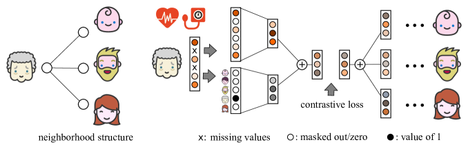
Figure 2: Illustration of the embedding propagation framework for missing data.

Learning Representations for Missing Data

Two characteristics of Ep make it suitable for the problem of learning representations for missing data. First, it supports an arbitrary number of attribute types, and one can learn missing data representations tailored to attribute types. Second, Ep’s learning principle is based on reconstructing each node’s attribute representation from neighboring nodes’ attribute representations, and this makes it highly suitable for settings wherein a number of nodes have missing data. During training, Ep learns how to reconstruct the missing data representation based on a contrastive loss between representations of existing attribute types and, therefore, can learn how to reconstruct a representation when data is missing.

For every attribute type $i$ and for every node $v\in V=\{1,...,|V|\}$ of the graph we have an input feature vector $\mathbf{x}$. Based on this vector, we create two feature vectors. The first feature vector $\mathbf{x}_{1}$ is identical to $\mathbf{x}$ except that all missing values are masked out. The second feature vector $\mathbf{x}_{2}\in\mathbb{R}^{|V|}$ is either (1) all zeros if there are no missing attribute values for attribute type $i$ or (2) all zeros except for the position $v$ which is set to $1$. The vector $\mathbf{x}_{2}$ indicates whether data is missing and and is used to learn a latent representation for nodes with missing data. These two vectors are then fed into two encoding functions $\mathtt{f}^{1}_{i}$ and $\mathtt{f}^{2}_{i}$ whose parameters are learned independently from each other. For each input, the output vectors of the encoding functions are added element-wise, and the resulting vector is used in the margin-based contrastive loss function. Therefore, for every attribute type $i$ we have $\mathbf{x}^{\prime}=\mathtt{f}_{i}(\mathbf{x})=\mathtt{f}^{1}_{i}(\mathbf{x}_{1})+\mathtt{f}^{2}_{i}(\mathbf{x}_{2})=\mathbf{x}_{1}^{T}\mathbf{W}^{1}_{i}+\mathbf{x}_{2}^{T}\mathbf{W}^{2}_{i}$. The $\mathtt{f}^{2}_{i}$ encoding functions amount to embedding lookup tables. We refer to this instance of Ep as EP-md (for “EP-missing data”).

Figure 2 illustrates our approach to learning separate representations for observed and missing attribute labels. Since the contrastive loss compares representations that are computed both based on missing and observed data, the two representations influence each other. If for some node $v$ and attribute type $i$ we have missing data, the representation of that missing data is influenced by the representations of observed and missing data of attribute type $i$ by neighboring nodes. Thus, the missing data representations are also propagated during the message passing.

As mentioned in Section 2, we standardize features to have a mean of $0$; $\mathbf{x}_{2}$ allows EP-md to distinguish between observed $0$s and missing values which have been masked.

Missing data mechanisms

Missing data is often assumed to result from mechanisms such as Missing (Completely) at Random (MAR and MCAR) or Not Missing at Random (NMAR) (?). In contrast to methods like multiple imputation by chained equations (?), EP-md does not estimate (representations of) missing attributes based on other observed attributes; rather, it leverages the affinity graph to learn representations based on the same attribute observed for similar nodes. Thus, EP-md does not assume an explicit missingness mechanism. We leave exploration of the statistical missingness properties of EP-md to future work.

Generating Patient Representations

Once the learning of attribute type representations has finished, Ep computes a vector representation for each patient node $v$ from the vector representations of $v$’s attribute types. In this work, the patient representation is the concatenation of the attribute type representations:

$$\mathbf{v}=\mathtt{concat}\left[\mathbf{h}_{1}(v),...,\mathbf{h}_{k}(v)\right].$$ (4)

Since we have modeled missing data explicitly, the latent representations $\mathbf{h}_{i}(v)$ exist for every node in the graph and every attribute type $i$. We also evaluate a patient representation built from both the raw features and the learned representations:

$$\mathbf{v}=\mathtt{concat}\left[\mathbf{h}_{1}(v),...,\mathbf{h}_{k}(v),\mathbf{x}_{1}(v),...,\mathbf{x}_{k}(v)\right],$$ (5)

where $\mathbf{x}_{i}(v)$ is the raw input for attribute type $i$ and node $v$.

4 Experiments

We first describe our experimental design. We then present and discuss our results on the three patient outcome prediction tasks.

Hyperparameters and computing environment

For EP-md, we use $200$ iterations of training with mini-batches of size $256$. We embed all attributes in a $32$-dimensional space. We set the margin $\gamma=5$, and we solved the EP-md optimization problem using Adam with a learning rate of $1e-3$. EP-md was implemented in Keras using TensorFlow as the backend. All experiments were run on computers with $128$GB RAM, four quad-core $2.8$ GHz CPU, and a TitanX GPU. The computing cluster was in a shared environment, so we do not report running times in this evaluation. In all cases, though, the running times were modest, ranging from a few minutes up to about an hour for learning embeddings for all episodes for a single attribute type.

Baseline and downstream models

Prior work has shown that linear models perform admirably compared to much more sophisticated methods on these and similar benchmark problems (?; ?; ?). Thus, we use (multi-class) logistic regression as a base model for mort and DD and ridge regression as the base model for LoS. Both implementations are from scikit-learn (?).

We leave a more comprehensive comparison to complex models such as long short-term memory networks (LSTMs) as future work. However, we do include comparison to previously-published performance of an LSTM (?) on mort. For a baseline, missing values are replaced with the mean of the respective feature. This completed data is then used to train the base model. We compare the baselines to learning embeddings with EP-md followed by the same supervised learning approach (either logistic or ridge regression). We select all hyperparameters based on cross-validation (please see Appendix D for more details). Ep has been shown to outperform methods like DeepWalk (?) and graph convolutional networks (?); thus, we do not compare to those methods in this work.

Construction of the affinity graph

An integral component of EP-md is the affinity graph; it gives a mechanism to capture domain knowledge about the similarity of the nodes to which traditional machine learning approaches do not have access. In this work, since the goal is always to make a prediction about the outcome of an episode, each node in the graph corresponds to an episode.

As described in Section 2, we extract the admission type, location, and initial diagnosis about each episode. We base the construction of our graph on the text from these fields. In particular, we concatenate the three fields to form a “document” for each episode. Next, we use $\mathtt{fastText}$ to learn custom word embeddings via skipgrams from this corpus. We then use these to calculate a single embedding (a “sentence vector”; please see the software documentation for more details) for each episode. We then define the similarity between two episodes $i$ and $j$ as $s_{i,j}=\exp{\{-d_{i,j}\}}\text{,}$ where $d_{i,j}$ is the Euclidean distance between the respective embeddings. Finally, we connect all pairs of episodes for which $s_{i,j}>0.9$.

Data partitioning

(?) created a standard training and testing set split of episodes. The training set includes $17~{}869$ episodes; the testing set includes $3~{}233$ episodes. While modest in comparison to some datasets considered in the machine learning community, this dataset is huge compared to many datasets presented in the medical literature. Thus, we also consider the ability to generalize to the test set when outcome information is available for only smaller numbers of training episodes. In particular, we draw subsets of varying size (see Figure 3) and only observe the class label for those episodes. As described in Section 3, EP-md can still take advantage of the unlabeled episodes. On the other hand, completely supervised methods can only use the episodes with class labels. We note that our predictions are always made $48$ hours after admission. We ensure that our learning only considers information that would be available in such a realistic scenario.

Evaluation metrics

We use standard metrics for evaluation. We use the area under the receiver operating characteristic curve (AuROC) to evaluate mort, mean absolute error (MAE) to evaluate LoS, and a multi-class generalization of AuROC (mc-AuROC) (?) for DD.

Results

Time series modality only

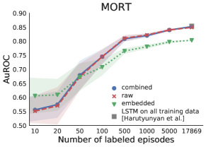
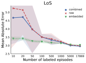
All data modalities

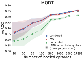
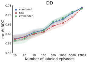
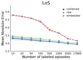
Figure 3: The respective performance of using only the “raw” features, only the “embedded” episode representations, or the “combined” features for training a logistic (for mort and DD) or ridge (for LoS) regression model using either the single time series modality (top) or all four data modalities (bottom) as input. The x-axis gives the number of labeled training episodes (out of a total of $17~{}869$ episodes in the full training set). $20$ random samples of each subset size were evaluated for each representation. The markers give the mean performance on the entire test set, and the shaded regions show one standard deviation above and below the mean. For mort, we also indicate the performance of the best single-task LSTM used in (?) Please note that higher AuROC values are better (for mort and DD), while lower MAE values are better (for LoS).

We first consider the impact of learning embeddings on only the time series data present in the original benchmarks for use in downstream prediction. Figure 3(top) compares the performance of the raw baseline (using just the hand-crafted features) compared to first learning representations of the time series attribute type using EP-md (embedded). We also include a third strategy (combined) in which we combine the original features with the representations learned by EP-md as described in Section 3. (Please see Appendix E for detailed tables of all results.)

As the figure shows, the embeddings are particularly helpful in small-data scenarios for mort and LoS. Prior work in the graph-embedding community has observed similar phenomena, so our findings are in line with that existing work. The embeddings are particularly well-suited for LoS. Indeed, this is the only task in this single data modality setting in which combined meaningfully differs from raw.

We observed that raw exhibits particularly high variance in performance for small subsample sizes for LoS, while the variance for embedded are in line with the other settings. This case particularly highlights the ability of EP-md to reduce noise and improve performance in missing data scenarios, even when only a single modality is available.

These results also show that both combined and raw match state-of-the-art performance by LSTMs reported in prior work (?). Further, the LSTMs were trained in a completely supervised manner; thus, their performance is expected to deteriorate when using smaller training sets (?).

Multi-modal data

We then extend our analysis to the multi-attribute case. As described in Section 3, we use EP-md to learn embeddings for each of the four attribute types (time series features, text notes, demographics, and episode identity within the graph) independently. The final representation for the episode is the concatenation of all attribute type representations. For raw, we used standard text (term-frequency inverse document-frequency) and categorical (one-hot encoding) variable preprocessing. We construct the graph for EP-md using additional information about the episode admission (see Section 2). We also encode these data as categorical variables and include them for raw.

Figure 3(bottom) shows the performance after adding the additional attributes. Relative to their performance in the single-attribute setting, the performance for all three representations improves across nearly all tasks and observed episode subsets. For mort, as in the single-attribute case, embedded is clearly worse than using only the hand-crafted features; however, combining the embeddings with the raw features does no harm, and combined and raw perform virtually identically. Both mildly surpass the state-of-the-art results previously reported (?). The combined representation benefits significantly from the additional data attributes on the LoS task. Indeed, it outperforms both raw and embedded across all subsample sizes. In this task, combined effectively uses information from both raw and embedded, rather than simply learning to use the best, as seems the case in other settings.

Finally, all of the representations show significant improvement in the DD task when the additional modalities are available. Both embedded and combined significantly outperform raw for several of the subset sizes.

Statistical significance

Across all of the sample sizes, embedded is significantly outperformed by raw (paired sample t-test, Benjamini-Hochberg multiple-test corrected $p\text{-value}$ $<0.05$) and combined on the DD task in the single-modality settings. Both are also significantly better than embedded on mort in the multiple modality setting. On the other hand, in the multi-modal setting for LoS, embedded is significantly better than raw, and combined is significantly better than both. combined is also significantly better than raw in the multi-modal case on DD.

Impact of missing data

We hypothesize that embedded outperforms raw for instances with many missing values. Figure 4(left) confirms that, on the LoS task, for patients with few missing values, embedded and raw perform similarly. embedded outperforms raw the most in cases with $5$ to $10$ missing values ($\approx 20-40\%$); embedded continues to result in more accurate predictions for larger numbers of missing values, but the difference is not as stark.

We next consider the effect on prediction quality when specific features are missing. As shown in Figure 4(right), predictions based on embedded for LoS are similar regardless of whether most features are observed or missing; this suggests that EP-md effectively propagates useful information about missing features throughout the graph.

On the other hand, raw features lead to worse predictions when most of the less-frequent features are observed. This helps explain the better performance of embedded compared to raw on LoS; embedded-based predictions effectively use all of the available information, while models trained on raw are actually misled by rare attributes.

For raw, missing temperature led to the worst change in performance, while features related to the Glasgow coma scale had the largest negative effect for embedded. raw results in much better predictions when the capilary refill rate is missing (the bottom left marker in the plot). All of the MAE losses are given in Appendix F.

Feature importance

As previously described, EP-md allows us to identify the original features which most influence predictions. For LoS, we consider the average contribution to the final prediction across all test instances (based on the learned model coefficients and embeddings for each instance) as the importance for each feature. The plots in Appendix G show that temperature and pH are the most influential features for embedded-based predictions; the Glasgow coma scale features are the next most influential. Interestingly, the contributions of temperature and pH are similar regardless of whether they are observed. This again suggests that EP-md effectively propagates useful information about missing features. On the other hand, the Glasgow coma scale features contribute much less when they are not observed.

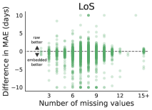
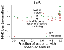
Figure 4: (left) Difference in the mean absolute error on all test instances when using $100$ labeled samples for training. Negative values indicate that embedded produced better predictions that raw. (right) Comparison of the MAE when a feature is observed for a test instance compared to when it is missing. The x-axis gives the percentage of patients for which a specific feature was observed; the y-axis shows the difference between the MAE for instances when the feature is observed and when it is not. Each marker corresponds to one feature. A negative value indicates that predictions are more accurate for patients where the feature is missing.

5 Related Work

We review some of the most related work on missing data and representation learning for clinical datasets.

Missing data in clinical datasets

A large body of recent research has addressed the problem of predicting patient outcomes from multivariate time series. The availabiliy of large, high-quality datasets like MIMIC-III (?) and those made available through the Computing in Cardiology challenges (?) has surely spurred some of this work. This data entails missingness almost by design since different vital signs are typically observed at different frequencies. Methodologically, much of this work  (?; ?; ?; ?; ?; ?; ?) borrows from and extends recent developments in the deep learning community, such as long short-term memory (LSTM) networks (?). Some Bayesian methods (?; ?; ?) have also been developed. While our approach builds upon this work, such as by extending previously-described hand-crafted features (?; ?), the use of multi-modal data is clearly novel in our work compared to this body. Further, our novel message passing scheme for missing data distinguishes our contribution from this work.

Representation learning and clinical data

A second approach to predicting patient outcomes from EHRs has instead focused on learning representations from discrete observations, such as prescribed medications and International Classification of Diseases (ICD) codes assigned during billing. Much of this work (?; ?; ?) builds on the recent successes of deep learning to include domain-specific background knowledge. Some recent work (?) has also considered text modalities, though they use word co-occurrence matrices.

Our use of a graph to explicitly capture similarity relationships among patients distinguishes our work from these prior approaches. Additionally, these methods typically do not consider the impact of missing data. In contrast, we explicitly learn a representation of the missing observations.

6 Discussion

We have presented an approach for learning representations for ICU episodes from multimodal data, which could come from EHRs. Our approach extends an existing representation learning framework, embedding propagation (?), to handle missing data. Empirically, we demonstrate that our approach outperforms a state-of-the-art baseline in predicting hospital visit duration and discharge destination when multiple attribute types are available; when combined with hand-crafted features, our approach is competitive with long short-term memory networks for in-hospital mortality prediction.

Future developments of our approach include extending both the considered tasks and data included in the model. We did not consider the “computational phenotyping” task (?; ?) in this work. This is typically formulated as a multi-label classification problem; the representations learned with EP-md can be combined with standard models for that setting. Currently, our model does not incorporate medications, procedures and treatments that occur during an episode; clearly, these have bearing on the patient outcomes. Since such data is available in MIMIC-III, we plan to integrate appropriate attribute types for these data.

References

- [Azur et al. 2011] Azur, M. J.; Stuart, E. A.; Frangakis, C.; and Leaf, P. J. 2011. Multiple imputation by chained equations: what is it and how does it work? International Journal of Methods in Psychiatric Research 20(1):40–49.
- [Barnes et al. 2016] Barnes, S.; Hamrock, E.; Toerper, M.; Siddiqui, S.; and Levin, S. 2016. Real-time prediction of inpatient length of stay for discharge prioritization. Journal of the American Medical Informatics Association 23(e1):e2–e10.
- [Brauer et al. 2008] Brauer, S. G.; Bew, P. G.; Kuys, S. S.; Lynch, M. R.; and Morrison, G. 2008. Prediction of discharge destination after stroke using the motor assessment scale on admission: A prospective, multisite study. Archives of Physical Medicine and Rehabilitation 89(6):1061–1065.
- [Che et al. 2015] Che, Z.; Kale, D.; Li, W.; Bahadori, M. T.; and Liu, Y. 2015. Deep computational phenotyping. In Proc. KDD.
- [Choi et al. 2016a] Choi, E.; Bahadori, M. T.; Schuetz, A.; Stewart, W. F.; and Sun, J. 2016a. Doctor AI: Predicting clinical events via recurrent neural networks. In Proc. MLHC.
- [Choi et al. 2016b] Choi, E.; Bahadori, M. T.; Sun, J.; Kulas, J.; Schuetz, A.; and Stewart, W. 2016b. RETAIN: An interpretable predictive model for healthcare using reverse time attention mechanism. In Proc. NIPS.
- [Choi et al. 2017] Choi, E.; Schuetz, A.; Stewart, W. F.; and Sun, J. 2017. Using recurrent neural network models for early detection of heart failure onset. Journal of the American Medical Informatics Association 24(2):361–370.
- [Choi, Chiu, and Sontag 2016] Choi, Y.; Chiu, C. Y.-I.; and Sontag, D. 2016. Learning low-dimensional representations of medical concepts. In AMIA Summits on Translational Science Proceedings, 41–50.
- [García-Durán and Niepert 2017] García-Durán, A., and Niepert, M. 2017. Learning graph representations with embedding propagation. In Proc. NIPS.
- [Gilmer et al. 2017] Gilmer, J.; Schoenholz, S. S.; Riley, P. F.; Vinyals, O.; and Dahl, G. E. 2017. Neural message passing for quantum chemistry. In Proc. ICML.
- [Hamilton, Ying, and Leskovec 2017] Hamilton, W. L.; Ying, R.; and Leskovec, J. 2017. Inductive representation learning on large graphs. Proc. NIPS.
- [Hammerla et al. 2015] Hammerla, N. Y.; Fisher, J.; Andras, P.; Rochester, L.; Walker, R.; and Ploetz, T. 2015. PD disease state assessment in naturalistic environments using deep learning. In Proc. AAAI.
- [Hand and Till 2001] Hand, D., and Till, R. 2001. A simple generalisation of the area under the ROC curve for multiple class classification problems. Machine Learning 45(2):171–186.
- [Harutyunyan et al. 2017] Harutyunyan, H.; Khachatrian, H.; Kale, D. C.; and Galstyan, A. 2017. Multitask learning and benchmarking with clinical time series data. arXiv:1703.07771 [stat.ML].
- [Hochreiter and Schmidhuber 1997] Hochreiter, S., and Schmidhuber, J. 1997. Long short-term memory. Neural Computation 9(8):1735–1780.
- [Johnson et al. 2016] Johnson, A. E.; Pollard, T. J.; Shen, L.; wei H. Lehman, L.; Feng, M.; Ghassemi, M.; Moody, B.; Szolovits, P.; Celi, L. A.; and Mark, R. G. 2016. MIMIC-III, a freely accessible critical care database. Scientific Data 3(160035).
- [Kipf and Welling 2017] Kipf, T. N., and Welling, M. 2017. Semi-supervised classification with graph convolutional networks. In Proc. ICLR.
- [Lasko, Denny, and Levy 2013] Lasko, T. A.; Denny, J. C.; and Levy, M. A. 2013. Computational phenotype discovery using unsupervised feature learning over noisy, sparse, and irregular clinical data. PLoS ONE 8(6):e66341.
- [Lehman et al. 2008] Lehman, L. H.; Saeed, M.; Moody, G.; and Mark, R. 2008. Similarity-based searching in multi-parameter time series databases. Computers in Cardiology 35:653–656.
- [Lipton et al. 2016] Lipton, Z. C.; Kale, D. C.; Elkan, C.; and Wetzel, R. 2016. Learning to diagnose with LSTM recurrent neural networks. In Proc. ICLR.
- [Lipton, Kale, and Wetzel 2016] Lipton, Z. C.; Kale, D. C.; and Wetzel, R. 2016. Modeling missing data in clinical time series with RNNs. In Proc. MLHC.
- [Marlin et al. 2012] Marlin, B. M.; Kale, D. C.; Khemani, R. G.; and Wetzel, R. C. 2012. Unsupervised pattern discovery in electronic health care data using probabilistic clustering models. In Proceedings of the ACM SIGHIT International Health Informatics Symposium.
- [Mauthe et al. 1996] Mauthe, R. W.; Haaf, D. C.; Hayn, P.; and Krall, J. M. 1996. Predictors for patient discharge destination after elective anterior cervical discectomy and fusion. Archives of Physical Medicine and Rehabilitation 77(1):10–13.
- [Pedregosa et al. 2011] Pedregosa, F.; Varoquaux, G.; Gramfort, A.; Michel, V.; Thirion, B.; Grisel, O.; Blondel, M.; Prettenhofer, P.; Weiss, R.; Dubourg, V.; Vanderplas, J.; Passos, A.; Cournapeau, D.; Brucher, M.; Perrot, M.; and Duchesnay, E. 2011. Scikit-learn: Machine learning in Python. Journal of Machine Learning Research 12:2825–2830.
- [Perozzi, Al-Rfou, and Skiena 2014] Perozzi, B.; Al-Rfou, R.; and Skiena, S. 2014. DeepWalk: Online learning of social representations. In Proc. KDD.
- [Rajkomar et al. 2018] Rajkomar, A.; Oren, E.; Chen, K.; Dai, A. M.; Hajaj, N.; Liu, P. J.; Liu, X.; Sun, M.; Sundberg, P.; Yee, H.; Zhang, K.; Duggan, G. E.; Flores, G.; Hardt, M.; Irvine, J.; Le, Q.; Litsch, K.; Marcus, J.; Mossin, A.; Tansuwan, J.; Wang, D.; Wexler, J.; Wilson, J.; Ludwig, D.; Volchenboum, S. L.; Chou, K.; Pearson, M.; Madabushi, S.; Shah, N. H.; Butte, A. J.; Howell, M.; Cui, C.; Corrado, G.; and Dean, J. 2018. Scalable and accurate deep learning for electronic health records. npj Digital Medicine 1(18).
- [Ramachandran, Liu, and Le 2017] Ramachandran, P.; Liu, P. J.; and Le, Q. V. 2017. Unsupervised pretraining for sequence to sequence learning. In Proc. EMNLP.
- [Rubin 1976] Rubin, D. B. 1976. Inference and missing data. Biometrika 63(3):581–592.
- [Silva et al. 2012] Silva, I.; Moody, G.; Scott, D. J.; Celi, L. A.; and Mark, R. G. 2012. Predicting in-hospital mortality of patients in ICU: The PhysioNet/computing in cardiology challenge 2012. Computing in Cardiology 39:245–248.
- [Suresh, Szolovits, and Ghassemi 2016] Suresh, H.; Szolovits, P.; and Ghassemi, M. 2016. The use of autoencoders for discovering patient phenotypes. In NIPS Workshop on Machine Learning for Health.
- [Wee, Bagg, and Palepu 1999] Wee, J. Y.; Bagg, S. D.; and Palepu, A. 1999. The Berg balance scale as a predictor of length of stay and discharge destination in an acute stroke rehabilitation setting. Archives of Physical Medicine and Rehabilitation 80:448–452.