Mutual Information of Wireless Channels
and Block-Jacobi Ergodic Operators

Abstract

Shannon’s mutual information of a random multiple antenna and multipath time varying channel is studied in the general case where the process constructed from the channel coefficients is an ergodic and stationary process which is assumed to be available at the receiver. From this viewpoint, the channel can also be represented by an ergodic self-adjoint block-Jacobi operator, which is close in many aspects to a block version of a random Schrödinger operator. The mutual information is then related to the so-called density of states of this operator. In this paper, it is shown that under the weakest assumptions on the channel, the mutual information can be expressed in terms of a matrix-valued stochastic process coupled with the channel process. This allows numerical approximations of the mutual information in this general setting. Moreover, assuming further that the channel coefficient process is a Markov process, a representation for the mutual information offset in the large Signal to Noise Ratio regime is obtained in terms of another related Markov process. This generalizes previous results from Levy et.al. [18, 19]. It is also illustrated how the mutual information expressions that are closely related to those predicted by the random matrix theory can be recovered in the large dimensional regime.

Keywords : Ergodic Jacobi operators, Ergodic wireless channels, Large random matrix theory, Markovian channels, Shannon’s mutual information.

1 Introduction

In order to introduce the problem that we shall tackle in this paper, we consider the example of a wireless communication model on a time and frequency selective channel that is described by the equation

$$y_{n}=\sum_{\ell=0}^{L}c_{n,\ell}s_{n-\ell}+v_{n},$$ (1)

where $L$ is the channel degree, where the complex numbers $s_{n}$, $y_{n}$ and $v_{n}$ represent respectively the transmitted signal, the received signal, and the additive noise at the moment $n$, and where the vector $C_{n}=[c_{n,0},\ldots,c_{n,L}]^{\mathsf{T}}\in\mathbb{C}^{L+1}$ contains the channel’s coefficients at the moment $n$. In a mobile environment, the sequence $(C_{n})$ is often modeled as a random ergodic process such as ${{\mathbb{E}}}\|C_{0}\|^{2}<\infty$ (here we take $\|\cdot\|$ as the Euclidean norm). Assuming that this process is available at the receiver site, our purpose is to study Shannon’s mutual information of this channel under the generic ergodicity assumption. By stacking $n-m+1$ elements of the received signal, where $m,n\in\mathbb{Z}$ and $m\leq n$, we get the vector model $\begin{bmatrix}y_{m},\ldots,y_{n}\end{bmatrix}^{\mathsf{T}}={\mathsf{B}}_{m,n}\begin{bmatrix}s_{m-L},\ldots,s_{n}\end{bmatrix}^{\mathsf{T}}+\begin{bmatrix}v_{m},\ldots,v_{n}\end{bmatrix}^{\mathsf{T}}$ with

$${\mathsf{B}}_{m,n}=\begin{bmatrix}c_{m,L}&\cdots&c_{m,0}\\ &\ddots&&\ddots\\ &&c_{n,L}&\cdots&c_{n,0}\end{bmatrix}.$$

Let $\rho>0$ be a parameter that represents the Signal to Noise Ratio (SNR). Considering the matrix/vector model above, and putting some standard assumptions on the statistics of the processes $(s_{n})$ and $(v_{n})$ (see below), this mutual information is written as

$${\mathcal{I}}_{\rho}=\operatorname*{aslim}_{n-m\to\infty}\frac{\log\det(\rho{\mathsf{B}}_{m,n}{\mathsf{B}}_{m,n}^{*}+I_{n-m+1})}{n-m+1}=\lim_{n-m\to\infty}\frac{{{\mathbb{E}}}\log\det(\rho{\mathsf{B}}_{m,n}{\mathsf{B}}_{m,n}^{*}+I_{n-m+1})}{n-m+1},$$ (2)

where ${\mathsf{B}}_{m,n}^{*}$ is the matrix adjoint of ${\mathsf{B}}_{m,n}$, and where the existence and the equality of both the limits above (“$\operatorname*{aslim}$” stands for the almost sure limit) are essentially due to the ergodicity of $(C_{n})$.

The natural mathematical framework for studying this limit is provided by the ergodic operator theory in the Hilbert space $\ell^{2}(\mathbb{Z})$, for whom a very rich literature has been devoted in the field of statistical physics [25]. In our situation, ${\mathsf{B}}_{m,n}$ is a finite rank truncation of the operator ${\mathsf{B}}$ represented by the doubly infinite matrix

$${\mathsf{B}}=\begin{bmatrix}\ddots&&\ddots\\ &c_{n,L}&\cdots&c_{n,0}\\ &&\ddots&&\ddots\end{bmatrix}.$$

Thanks to the ergodicity of $(C_{n})$, it is known that the spectral measure (or eigenvalue distribution) of the matrix ${\mathsf{B}}_{m,n}{\mathsf{B}}_{m,n}^{*}$ converges narrowly in the almost sure sense to a deterministic probability measure called the density of states of the self-adjoint operator ${\mathsf{B}}{\mathsf{B}}^{*}$, where ${\mathsf{B}}^{*}$ is the adjoint of ${\mathsf{B}}$. This convergence leads to the convergences in (2).

In statistical physics, the study of the density of states has focused most frequently on the Jacobi (or tridiagonal) ergodic operators which are associated to the so-called discrete Schrödinger equation in a random environment. In this framework, the Herbert-Jones-Thouless formula [7, 25] provides a means of characterizing the density of states of an ergodic Jacobi operator, in connection with the so-called Lyapounov exponent associated with a certain sequence of matrices.

In the context of the wireless communications that is of interest here, it turns out that the use of the Thouless formula is possible when one considers ${\mathsf{B}}{\mathsf{B}}^{*}$ as a block-Jacobi operator. This idea was developed by Levy et al. in [19]. The expression of the mutual information that was obtained in [19] was also used to perform a large SNR asymptotic analysis so as to obtain bounds on the mutual information in this regime.

In this paper, we take another route to calculate the mutual information. The expression we obtain for $\mathcal{I}_{\rho}$ in Theorem 1 below involves an ergodic process which is coupled with the channel process, and appears to be more tractable than the expression based on the top Lyapounov exponent provided in [19]. We moreover exploit the obtained expression for $\mathcal{I}_{\rho}$ to study two asymptotic regimes: we first consider the large SNR regime in a Markovian setting, and obtain an exact representation for the constant term in the expansion of ${\mathcal{I}}_{\rho}$ for large $\rho$. We also consider a regime where the dimensions of the blocks of our block-Jacobi operator converge to infinity; the expression of the mutual information that we recover is then closely related to what is obtained from random matrix theory [17, 12]. In the context of the example described by Equation (1), this asymptotic regime amounts to $L$ converging to infinity. Beyond this example, the large dimensional analysis can also be used to analyze the behavior of the mutual information of time and frequency selective channels in the framework of the massive Multiple Input Multiple Output (MIMO) systems ([22]), which are destined to play a dominant role in the future wireless cellular techniques/standards.

Organisation of the paper.

In Section 2, after stating precisely our communication model and our standing assumption, we provide our main result (Theorem 1). We then consider the large SNR regime in a Markovian setting (Theorem 2) along with some cases where the assumptions for this theorem to hold true are satisfied. In Section 3 we illustrate Theorems 1 and 2 with numerical experiments. There we also state our result on the large dimensional regime, which is related with one of the channel models considered in this section. The next sections are devoted to the proofs.

2 Problem description and statement of the results

2.1 The model

The model herein is well-suited for the block-Jacobi formalism that we use in the remainder. Given two positive integers $N$ and $K$, we consider the wireless transmission model

$$Y_{n}={\mathsf{F}}_{n}S_{n-1}+{\mathsf{G}}_{n}S_{n}+V_{n}$$ (3)

with $n\in\mathbb{Z}$ and where:

• $(Y_{n})_{n\in\mathbb{Z}}$ represents the $\mathbb{C}^{N}$-valued sequence of received signals.

• $(S_{n})_{n\in\mathbb{Z}}$ is the $\mathbb{C}^{K}$-valued sequence of transmitted information symbols.

• $({\mathsf{F}}_{n},{\mathsf{G}}_{n})_{n\in\mathbb{Z}}$ with ${\mathsf{F}}_{n},{\mathsf{G}}_{n}\in\mathbb{C}^{N\times K}$ is a matrix representation of a random wireless channel.

• $(V_{n})_{n\in\mathbb{Z}}$ is the additive noise.

Let us first give a few examples which fit with this transmission model.

The multipath single antenna fading channel.

The channel described by Equation (1) is a particular case of this model. When $L>0$, we put

$$Y_{n}:=\begin{bmatrix}y_{nL}\\ \vdots\\ y_{nL+L-1}\end{bmatrix},\quad S_{n}:=\begin{bmatrix}s_{nL}\\ \vdots\\ s_{nL+L-1}\end{bmatrix},\quad V_{n}:=\begin{bmatrix}v_{nL}\\ \vdots\\ v_{nL+L-1}\end{bmatrix},\quad N:=K:=L,$$ (4)

and ${\mathsf{F}}_{n},{\mathsf{G}}_{n}\in\mathbb{C}^{L\times L}$ are the upper triangular and lower triangular matrices defined as

$$\left[\begin{array}[]{c|c}{\mathsf{F}}_{n}&{\mathsf{G}}_{n}\end{array}\right]:=\left[\begin{array}[]{ccc|ccc}c_{nL,L}&\cdots&c_{nL,1}&c_{nL,0}&&\\ &\ddots&\vdots&\vdots&\ddots&\\ &&c_{nL+L-1,L}&c_{nL+L-1,L-1}&\cdots&c_{nL+L-1,0}\end{array}\right].$$ (5)

When $L=0$, we set instead $N:=K:=1$, $Y_{n}:=y_{n}$, $S_{n}:=s_{n}$, $V_{n}:=v_{n}$, ${\mathsf{F}}_{n}:=0$, and ${\mathsf{G}}_{n}:=c_{n,0}$.

In the multiple antenna variant of this model, the channel coefficients $c_{n,\ell}$ are $R\times T$ matrices, where $R$, resp. $T$, is the number of antennas at the receiver, resp. transmitter. In this case, the $N\times K$ matrices ${\mathsf{F}}_{n}$ and ${\mathsf{G}}_{n}$ given by Eq. (5) when $L>0$ are block triangular matrices with $N:=RL$ and $K:=TL$.

The Wyner multi-cell model.

Another instance of the transmission model introduced above is a generalization of the so-called Wyner multi-cell model considered in [14, 30], where the index $n$ now represents the space instead of representing the time. Assume that the Base Stations (BS) of a wireless cellular network are arranged on a line, and that each BS receives in a given frequency slot the signals of the $L+1$ users which are not too far from this BS. Alternatively, each user is also seen by $L+1$ BS. In this setting, the signal $y_{n}$ received by the BS $n$ is described by Eq. (1) (where the time parameter is now omitted), where $s_{n}$ is the signal emitted by User $n$, and where $c_{n,\ell}$ is the uplink channel carrying the signal of User $n-\ell$ to BS $n$.

Other domains than the time or the space domain, such as the frequency domain, can also be covered, see e.g. [29], which deals with a time and frequency selective model. Moreover, this could even address different connected domains as the Doppler-Delay (connected via the so-called Zak transform), as in [4, 3], which lead to modulation schemes that are considered as interesting candidates for the fifth generation (5G) wireless systems, as reflected in the references [13, 6].

2.2 General assumptions

The purpose of this work is to study Shannon’s mutual information between $(S_{n})$ and $(Y_{n})$ when the channel is known at the receiver. To this end, we consider the usual setting where:

• The information sequence $(S_{n})_{n\in\mathbb{Z}}$ is random i.i.d. with law $\mathcal{CN}(0,I_{K})$.

• The noise $(V_{n})_{n\in\mathbb{Z}}$ is i.i.d. with law $\mathcal{CN}(0,\rho^{-1}I_{N})$ for some $\rho>0$ that scales with the SNR.

• The random sequences $(S_{n})_{n\in\mathbb{Z}}$, $({\mathsf{F}}_{n},{\mathsf{G}}_{n})_{n\in\mathbb{Z}}$, and $(V_{n})_{n\in\mathbb{Z}}$ are independent.

Here and in the following, i.i.d. means “independent and identically distributed”, and $\mathcal{CN}(0,\Sigma)$ stands for the law of a centered complex Gaussian circularly symmetric vector with covariance matrix $\Sigma$. We also make the following assumptions on the process $({\mathsf{F}}_{n},{\mathsf{G}}_{n})_{n\in\mathbb{Z}}$ representing the channel:

Assumption 1.

The process $({\mathsf{F}}_{n},{\mathsf{G}}_{n})_{n\in\mathbb{Z}}$ is a stationary and ergodic process. Moreover,

$${{\mathbb{E}}}\|{\mathsf{F}}_{0}\|^{2}<\infty\quad\text{ and }\quad{{\mathbb{E}}}\|{\mathsf{G}}_{0}\|^{2}<\infty.$$ (6)

Note that the moment assumption (6) does not depend on the specific choice of the norm on the space of $N\times K$ complex matrices. In the remainder, we choose $\|\cdot\|$ to be the spectral norm.

Let us make precise the assumptions of stationarity and ergodicity. In the following we set for convenience

$$E:=\mathbb{C}^{N\times K}\times\mathbb{C}^{N\times K}$$ (7)

and consider the measure space $\Omega:=E^{\mathbb{Z}}$ equipped with its Borel $\sigma$–field ${\mathscr{F}}:={\mathscr{B}}(E)^{\otimes\mathbb{Z}}$. An element of $\Omega$ reads $\omega=\left(\ldots,(F_{-1},G_{-1}),(F_{0},G_{0}),(F_{1},G_{1}),\ldots\right)$ where $(F_{n},G_{n})$ is the $n^{\text{th}}$ coordinate of $\omega$, with $(F_{n},G_{n})\in E$. The shift ${\mathsf{T}}:\Omega\to\Omega$ acts as ${\mathsf{T}}\omega:=\left(\ldots,(F_{0},G_{0}),(F_{1},G_{1}),(F_{2},G_{2}),\ldots\right).$ The assumption that $({\mathsf{F}}_{n},{\mathsf{G}}_{n})_{n\in\mathbb{Z}}$ is an ergodic stationary process, seen as a measurable map from $(\Omega,{\mathscr{F}})$ to itself, means that the shift ${\mathsf{T}}$ is a measure preserving and ergodic transformation with respect to the probability distribution of the process $({\mathsf{F}}_{n},{\mathsf{G}}_{n})_{n\in\mathbb{Z}}$.

A fairly general stationary and ergodic model is provided by the following example.

Example 1.

In the single antenna and single path ($L=0$) fading channel case, the autoregressive (AR) statistical model has been considered as a realistic model for representing the Doppler effect induced by the mobility of the communicating devices. This model reads

$$c_{n,0}=\sum_{\ell=1}^{M}a_{\ell}c_{n-\ell,0}+u_{n},$$ (8)

where $M>0$ is the order of the AR channel process, $(u_{n})_{n\in\mathbb{Z}}$ is an i.i.d. driving process, and $(a_{1},\ldots,a_{M})$ are the constant AR filter coefficients, which can be tuned to meet a required Doppler spectral density (see, e.g., [2]).

In the multipath case, this model can be generalized to account for the presence of a power delay profile and the presence of correlations between the channel taps in addition to the Doppler effect. In this case, the channel coefficients vector $C_{n}=[c_{n,0},\ldots,c_{n,L}]^{\mathsf{T}}$ is written as

$$C_{n}=\sum_{\ell=1}^{M}A_{\ell}C_{n-\ell}+U_{n},$$ (9)

where $\{A_{1},\ldots,A_{M}\}$ is a collection of deterministic $(L+1)\times(L+1)$ matrices, and where $(U_{n})_{n\in\mathbb{Z}}$ is a $\mathbb{C}^{L+1}$–valued i.i.d. driving process. If the polynomial $\det(I-\sum_{\ell=1}^{M}z^{\ell}A_{\ell})$ does not vanish in the closed unit disc, it is well known that there exists a stationary and ergodic process whose law is characterized by (9), see e.g. [15, 23], leading to a stationary and ergodic process $({\mathsf{F}}_{n},{\mathsf{G}}_{n})_{n\in\mathbb{Z}}$ by recalling the construction of $\begin{bmatrix}{\mathsf{F}}_{n}\,|\,{\mathsf{G}}_{n}\end{bmatrix}$ given by Equation (5).

2.3 Mutual information and statement of the main result

In order to define the mutual information of the channel described by (3), define for any $m,n\in\mathbb{Z}$, $m\leq n$, the random matrix of size $(n-m+1)N\times(n-m+2)K$,

$${\mathsf{H}}_{m,n}:=\begin{bmatrix}{\mathsf{F}}_{m}&{\mathsf{G}}_{m}\\ &{\mathsf{F}}_{m+1}&{\mathsf{G}}_{m+1}\\ &&\ddots&\ddots\\ &&&{\mathsf{F}}_{n}&{\mathsf{G}}_{n}\end{bmatrix}.$$ (10)

For any fixed $\rho>0$, let ${\mathcal{I}}_{\rho}$ be given by

$$\mathcal{I}_{\rho} :=\operatorname*{aslim}_{n-m\to\infty}\frac{1}{(n-m+1)N}\log\det\left(I+\rho\,{\mathsf{H}}_{m,n}{\mathsf{H}}_{m,n}^{*}\right)$$

$$=\lim_{n-m\to\infty}\frac{1}{(n-m+1)N}{{\mathbb{E}}}\log\det\left(I+\rho\,{\mathsf{H}}_{m,n}{\mathsf{H}}_{m,n}^{*}\right).$$ (11)

As we shall briefly explain below, these two limits exist, are finite and equal, and do not depend on the way $n-m\to\infty$ due to the Assumption 1. As is well known, $\mathcal{I}_{\rho}$ is known to represent the required mutual information per component of our wireless channel, provided the input $S_{n}$ is as in Section 2.2, see [10]. The purpose of this paper is to study this quantity.

Remark 1.

In the Wyner multicell model introduced above, where the BS collaborate while the users do not, ${\mathcal{I}}_{\rho}$ represents the sum mutual information per component.

Denoting by ${\mathcal{H}}_{K}^{++}$, resp. ${\mathcal{H}}_{K}^{+}$, the cone of the Hermitian positive definite, resp. semidefinite, $K\times K$ matrices, we show that one can construct a stationary ${\mathcal{H}}_{K}^{++}$-valued process $({\mathsf{W}}_{n})_{n\in\mathbb{Z}}$ defined recursively and coupled with $({\mathsf{F}}_{n},{\mathsf{G}}_{n})_{n\in\mathbb{Z}}$ which allows a rather simple formula for the mutual information per component $\mathcal{I}_{\rho}$.

Theorem 1 (Mutual information of an ergodic channel).

If Assumption 1 holds true, then:

• There exists a unique stationary ${\mathcal{H}}_{K}^{++}$-valued process $({\mathsf{W}}_{n})_{n\in\mathbb{Z}}$ satisfying

  $${\mathsf{W}}_{n}=\left(I+\rho\,{\mathsf{G}}_{n}^{*}\left(I+\rho\,{\mathsf{F}}_{n}{\mathsf{W}}_{n-1}{\mathsf{F}}_{n}^{*}\right)^{-1}{\mathsf{G}}_{n}\right)^{-1}.$$ (12)

  In particular, the process $({\mathsf{W}}_{n})$ is ergodic.

• We have the representation for the mutual information per component:

  $$\mathcal{I}_{\rho}=\frac{1}{N}\Big{(}{{\mathbb{E}}}\log\det\left(I+\rho\,{\mathsf{F}}_{0}{\mathsf{W}}_{-1}{\mathsf{F}}_{0}^{*}\right)-{{\mathbb{E}}}\log\det{\mathsf{W}}_{0}\Big{)}.$$ (13)

• Given any matrix ${\mathsf{X}}_{-1}\in{\mathcal{H}}_{K}^{+}$, if one defines a process $({\mathsf{X}}_{n})_{n\in{{\mathbb{N}}}}$ by setting

  $${\mathsf{X}}_{n}:=\left(I+\rho\,{\mathsf{G}}_{n}^{*}\left(I+\rho\,{\mathsf{F}}_{n}{\mathsf{X}}_{n-1}{\mathsf{F}}_{n}^{*}\right)^{-1}{\mathsf{G}}_{n}\right)^{-1}$$ (14)

  for all $n\geq 0$, then we have

  $$\mathcal{I}_{\rho}=\lim_{n\to\infty}\frac{1}{nN}\sum_{\ell=0}^{n-1}\log\det\left(I+\rho\,{\mathsf{F}}_{\ell}{\mathsf{X}}_{\ell-1}{\mathsf{F}}_{\ell}^{*}\right)-\log\det{\mathsf{X}}_{\ell}\quad\text{a.s.}$$ (15)

The proof of Theorem 1 is provided in Section 4.

Remark 2.

As we will illustrate in Section 3, Theorem 1(c) yields an estimator for $\mathcal{I}_{\rho}$ that is less costly numerically than the naive one, due to the dimension of the involved matrices.

Remark 3.

The proof of Theorem 1 reveals that the moment assumption (6) can be weakened to

$${{\mathbb{E}}}\log(1+\|{\mathsf{F}}_{0}\|^{2})<\infty\qquad\text{ and }\qquad{{\mathbb{E}}}\log(1+\|{\mathsf{G}}_{0}\|^{2})<\infty.$$ (16)

The second moment assumption (6) is here to ensure that the received signal power is finite.

Remark 4.

An expression for ${\mathcal{I}}_{\rho}$ similar to the one given by Theorem 1 is obtained by Levy et.al. in [18] in the particular case where $N=1$ and where the process $({\mathsf{F}}_{n},{\mathsf{G}}_{n})$ is i.i.d.

2.4 Connection to block-Jacobi operators and previous results

Recall Eq. (10). Due to Assumption 1, it is well known, see [25], that there exists a deterministic probability measure $\mu$ that can defined by the fact that for each bounded and continuous function $f$ on $[0,\infty)$,

$$\frac{1}{(n-m+1)N}\operatorname{tr}f({\mathsf{H}}_{m,n}{\mathsf{H}}_{m,n}^{*})\xrightarrow[n-m\to\infty]{}\int f(\lambda)\,\mu(d\lambda)\quad\text{a.s.}$$ (17)

(here, $f$ is of course extended by functional calculus to the semi-definite positive matrices). The measure $\mu$ is intimately connected with the so-called ergodic self-adjoint block-Jacobi (or block-tridiagonal) operator ${\mathsf{H}}{\mathsf{H}}^{*}$, where ${\mathsf{H}}$ is the random linear operator acting on the Hilbert space $\ell^{2}(\mathbb{Z})$, and defined by its doubly-infinite matrix representation in the canonical basis $(e_{k})_{k\in\mathbb{Z}}$ of this space as

$${\mathsf{H}}=\begin{bmatrix}\ \ddots&\ddots\\ &{\mathsf{F}}_{-1}&{\mathsf{G}}_{-1}\\ &&{\mathsf{F}}_{0}&{\mathsf{G}}_{0}\\ &&&{\mathsf{F}}_{1}&{\mathsf{G}}_{1}\\ &&&&\ddots&\ddots\ \end{bmatrix}.$$ (18)

The random positive self-adjoint operator ${\mathsf{H}}{\mathsf{H}}^{*}$ is an ergodic operator in the sense of [25, Page 33] (see also [12]), and the measure $\mu$ is called its density of states. Recalling (11), it holds that

$$\mathcal{I}_{\rho}=\int\log(1+\rho\lambda)\,\mu(d\lambda),$$ (19)

where this limit is finite, due to the moment assumption (6) and a standard uniform integrability argument.

As said in the introduction, the Herbert-Jones-Thouless formula [7, 25] provides a means of characterizing the density of states of an ergodic Jacobi operator. In [19], Levy et al. develop a version of this formula that is well suited to the block-Jacobi setting of ${\mathsf{H}}{\mathsf{H}}^{*}$.

In this paper, we rather identify $\mathcal{I}_{\rho}$ by considering the resolvents of certain random operators built from the process $({\mathsf{F}}_{n},{\mathsf{G}}_{n})_{n\in\mathbb{Z}}$ instead of using the Herbert-Jones-Thouless formula. The expression we obtain for $\mathcal{I}_{\rho}$ involves the ergodic process $({\mathsf{W}}_{n})$ which is coupled with the process $({\mathsf{F}}_{n},{\mathsf{G}}_{n})_{n\in\mathbb{Z}}$ by Eq. (12). This approach is developed in Section 4.

2.5 The Markovian case and large SNR regime

First, assuming extra assumptions on the process $({\mathsf{F}}_{n},{\mathsf{G}}_{n})$, we obtain a description for the constant term (or mutual information offset) in the large SNR regime. Indeed, it often happens that there exists a real number $\kappa_{\infty}$ such that the mutual information per component admits the expansion as $\rho\to\infty$,

$$\mathcal{I}_{\rho}=\min(K/N,1)\log\rho+\kappa_{\infty}+o(1),$$ (20)

see e.g. [20]. Our next task is to prove this expansion indeed holds true and to derive an expression for the offset $\kappa_{\infty}$ when the process $({\mathsf{F}}_{n},{\mathsf{G}}_{n})_{n\in\mathbb{Z}}$ is further assumed to be a Markov process satisfying some regularity and moment assumptions. Namely, consider for any $n\in\mathbb{Z}$ the $\sigma$-field $\mathscr{F}_{n}:=\sigma(({\mathsf{F}}_{k},{\mathsf{G}}_{k})\;:k\leq n)$ and assume there exists a transition kernel $P:E\times{\mathscr{B}}(E)\to[0,1]$ such that, for any Borel function $f:E\to[0,\infty)$,

$${{\mathbb{E}}}\big{[}f({\mathsf{F}}_{n+1},{\mathsf{G}}_{n+1})|\mathscr{F}_{n}\big{]}=Pf(({\mathsf{F}}_{n},{\mathsf{G}}_{n})):=\int f(F,G)\,P\big{(}({\mathsf{F}}_{n},{\mathsf{G}}_{n}),dF\times dG\big{)}.$$ (21)

Besides $Pf(({\mathsf{F}},{\mathsf{G}}))$, we use the common notations from the Markov chains literature and also write $P(({\mathsf{F}},{\mathsf{G}}),A):=P\boldsymbol{1}_{A}(({\mathsf{F}},{\mathsf{G}}))$ for any Borel set $A\in{\mathscr{B}}(E)$; the iterated kernel $P^{n}$ stands for the Markov kernel defined inductively by $P^{n}f:=P(P^{n-1}f)$ with the convention that $P^{0}f:=f$; given any probability measure $\eta$ on $E$, we let $\eta P$ be the probability measure on $E$ defined as

$$\eta P(A):=\int P((F,G),A)\,\eta(dF\times dG),\qquad A\in{\mathscr{B}}(E).$$ (22)

The following assumption is formulated in the context where $N>K$. We denote as ${\mathcal{M}}(E)$ the space of Borel probability measures on the space $E$. Given a matrix $A$, the notations $\Pi_{A}$ and $\Pi_{A}^{\perp}$ refer respectively to the orthogonal projector on the column space $\operatorname{span}(A)$ of $A$, and to the orthogonal projector on $\operatorname{span}(A)^{\perp}$.

Assumption 2.

The process $({\mathsf{F}}_{n},{\mathsf{G}}_{n})_{n\in\mathbb{Z}}$ is a Markov process with transition kernel $P$ associated with a unique invariant probability measure $\theta\in{\mathcal{M}}(E)$, namely satisfying $\theta P=\theta$. Moreover,

• $P$ is Feller, namely, if $f:E\to{{\mathbb{R}}}$ is continuous and bounded, then so is $Pf$.

• ${{\mathbb{E}}}\|{\mathsf{F}}_{0}\|^{2}+{{\mathbb{E}}}\|{\mathsf{G}}_{0}\|^{2}<\infty$.

• ${{\mathbb{E}}}|\log\det({\mathsf{F}}_{0}^{*}{\mathsf{F}}_{0})|<\infty$.

• For every non-zero $v\in\mathbb{C}^{K}$, we have for $\theta$-a.e. $(F,G)\in E$ that

  $$\det(G^{*}F)\neq 0\qquad\text{and}\qquad\Pi_{G}^{\perp}Fv\neq 0\,.$$ (23)

Remark 5.

Since a Markov chain $({\mathsf{F}}_{n},{\mathsf{G}}_{n})_{n\in\mathbb{Z}}$ associated with a unique invariant probability measure is automatically ergodic, we see that Assumption 2 is stronger than Assumption 1 and thus Theorem 1 applies in this setting.

Remark 6.

If one assumes $({\mathsf{F}}_{n},{\mathsf{G}}_{n})_{n\in\mathbb{Z}}$ is a sequence of i.i.d random variables with law $\theta$ having a density on $E$, then it satisfies Assumption 2 (and hence Assumption 1) provided that the moment conditions Assumption 2(b)-(c) are satisfied. We also provide more sophisticated examples were Assumption 2 holds in Section 2.5.

Remark 7.

Since $\theta=\theta P$, Assumption 2(d) equivalently says that, for $\theta$-a.e. $({\mathsf{F}},{\mathsf{G}})$, (23) holds true for $P(({\mathsf{F}},{\mathsf{G}}),\cdot)$-a.e. $(F,G)\in E$. We will use this observation at several instances in the following.

Theorem 2 (The Markov case).

Let $N>K$. Then, under Assumption 2, the following hold true:

• There exists a unique stationary process $({\mathsf{Z}}_{n})_{n\in\mathbb{Z}}$ on ${\mathcal{H}}_{K}^{++}$ satisfying

  $${\mathsf{Z}}_{n}={\mathsf{G}}_{n}^{*}(I+{\mathsf{F}}_{n}{\mathsf{Z}}_{n-1}^{-1}{\mathsf{F}}_{n}^{*})^{-1}{\mathsf{G}}_{n}.$$ (24)

• We have, as $\rho\to\infty$,

  $$\mathcal{I}_{\rho}=\frac{K}{N}\log\rho+\kappa_{\infty}+o(1),$$ (25)

  where $\log\det({\mathsf{Z}}_{0}+{\mathsf{F}}_{1}^{*}{\mathsf{F}}_{1})$ is integrable, and

  $$\kappa_{\infty}:=\frac{1}{N}{{\mathbb{E}}}\log\det({\mathsf{Z}}_{0}+{\mathsf{F}}_{1}^{*}{\mathsf{F}}_{1}).$$ (26)

• Given any ${\mathsf{X}}_{-1}\in{\mathcal{H}}_{K}^{++}$, if we consider the process $({\mathsf{X}}_{n})_{n\in{{\mathbb{N}}}}$ defined recursively by

  $${\mathsf{X}}_{n}={\mathsf{G}}_{n}^{*}(I+{\mathsf{F}}_{n}{\mathsf{X}}_{n-1}^{-1}{\mathsf{F}}_{n}^{*})^{-1}{\mathsf{G}}_{n}\,,$$ (27)

  then we have, in probability,

  $$\kappa_{\infty}=\lim_{n\to\infty}\frac{1}{nN}\sum_{\ell=0}^{n-1}\log\det({\mathsf{X}}_{\ell}+{\mathsf{F}}_{\ell+1}^{*}{\mathsf{F}}_{\ell+1}).$$ (28)

The proof of Theorem 2 is provided in Section 5.

Remark 8 (The case $N\leq K$).

In the statement of Theorem 2, it is assumed that $N>K$. Let us say a few words about the case where $N<K$. In this case, assuming that $({\mathsf{F}}_{n},{\mathsf{G}}_{n-1})$ is a Markov chain, there is an analogue $(\widetilde{\mathsf{Z}}_{n})$ of the process $({\mathsf{Z}}_{n})$ satisfying the recursion

$$\widetilde{\mathsf{Z}}_{n}={\mathsf{F}}_{n}(I_{K}+{\mathsf{G}}_{n-1}^{*}\widetilde{\mathsf{Z}}_{n-1}^{-1}{\mathsf{G}}_{n-1})^{-1}{\mathsf{F}}_{n}^{*},$$ (29)

and adapting Assumption 2 to this new setting, we can show that ${\mathcal{I}}_{\rho}=\log\rho+\tilde{\kappa}_{\infty}+o(1)$, where

$$\tilde{\kappa}_{\infty}:=\frac{1}{N}{{\mathbb{E}}}\log\det(\widetilde{\mathsf{Z}}_{0}+{\mathsf{G}}_{0}{\mathsf{G}}_{0}^{*}).$$ (30)

This result can be obtained by adapting the proof of Theorem 2 in a straightforward manner.
The case $K=N$ is somehow singular and requires a specific treatment that will not be undertaken in this paper; see also the end of Section 5.1.2 for further explanations.

Remark 9.

In the case where $K=1$, $N>1$, and the process $({\mathsf{F}}_{n},{\mathsf{G}}_{n})_{n\in\mathbb{Z}}$ is i.i.d., we recover [18, Th. 2], where this result is obtained with the help of the theory of Harris Markov chains.

Examples where Assumption 2 is verified

In Proposition 3 below, the Markov property of the process $({\mathsf{F}}_{n},{\mathsf{G}}_{n})_{n\in\mathbb{Z}}$ is obvious, while in Proposition 4, it can be easily checked from Equation (5). Moreover, in both propositions, it is well known that the Markov process $({\mathsf{F}}_{n},{\mathsf{G}}_{n})_{n\in\mathbb{Z}}$ is an ergodic process satisfying Assumptions 2-(a) and 2-(b) [23]. We shall focus on Assumptions 2-(c) and 2-(d).

Proposition 3 (AR-model).

For $N>K$, assume $({\mathsf{F}}_{n},{\mathsf{G}}_{n})$ is the multidimensional ergodic AR process defined by the recursion

$$\begin{bmatrix}{\mathsf{F}}_{n}\\ {\mathsf{G}}_{n}\end{bmatrix}=A\begin{bmatrix}{\mathsf{F}}_{n-1}\\ {\mathsf{G}}_{n-1}\end{bmatrix}+\begin{bmatrix}U_{n}\\ V_{n}\end{bmatrix},$$ (31)

where $A\in\mathbb{C}^{2N\times 2N}$ is a deterministic matrix whose eigenvalue spectrum belongs to the open unit disk, and where $(U_{n},V_{n})_{n\in\mathbb{Z}}$ is an i.i.d. process on $E$ such that ${{\mathbb{E}}}\|U_{0}\|^{2}+{{\mathbb{E}}}\|V_{0}\|^{2}<\infty$. If the entries of the matrix $\begin{bmatrix}U_{n}\ V_{n}\end{bmatrix}$ are independent with their distributions being absolutely continuous with respect to the Lebesgue measure on $\mathbb{C}$, then Assumption 2-(d) is verified. If, furthermore, the densities of the elements of $U_{n}$ and $V_{n}$ are bounded, then, Assumption 2-(c) is verified.

Our second example is a particular multi-antenna version of the AR channel model of Example 1. This model is general enough to capture the Doppler effect, the correlations within each matrix coefficient of the channel, as well as the power profile of these taps.

Proposition 4 (MIMO multipath fading channel).

Given three positive integers $L,R$, and $T$ such that $R>T$, let $(C_{n})_{n\in\mathbb{Z}}$ be the $\mathbb{C}^{(L+1)R\times T}$-valued random process described by the iterative model

$$C_{n}=\begin{bmatrix}H_{0}\\ &\ddots\\ &&H_{L}\end{bmatrix}C_{n-1}+U_{n},$$ (32)

where the $\{H_{\ell}\}_{\ell=0}^{L}$ are deterministic $R\times R$ matrices whose spectra lie in the open unit disk, and where $(U_{n})_{n\in\mathbb{Z}}$ is an i.i.d. matrix process such that ${{\mathbb{E}}}\|U_{0}\|^{2}<\infty$. Let ${\mathsf{F}}_{n}$ and ${\mathsf{G}}_{n}$ be the $LR\times LT$ matrices defined as in (5) with $C_{n}=\begin{bmatrix}c_{n,0}^{\mathsf{T}}\ \cdots\ c_{n,L}^{\mathsf{T}}\end{bmatrix}^{\mathsf{T}}$, the $c_{n,\ell}$’s being $R\times T$ matrices. If the entries of $U_{n}$ are independent with their distributions being absolutely continuous with respect to the Lebesgue measure on $\mathbb{C}$, then Assumption 2-(d) is verified on the Markov process $({\mathsf{F}}_{n},{\mathsf{G}}_{n})_{n\in\mathbb{Z}}$. If, furthermore, the densities of the elements of $U_{n}$ are bounded, then, Assumption 2-(c) is verified.

Propositions 3 and 4 are proven in Section 5.4.

3 Numerical illustrations

We consider here a multiple antenna version of the multipath channel desribed in the introduction, see Equations (4)–(5). We assume the channel coefficient matrices $c_{n,\ell}$ satisfy the AR model $c_{n,\ell}=\alpha c_{n-1,\ell}+\sqrt{1-\alpha^{2}}a_{\ell}u_{n,\ell}$. Here the AR coefficient $\alpha$ takes the form $\alpha=\exp(-f_{\text{d}})$. The parameter $f_{\text{d}}$ represents the Doppler frequency, since it is proportional to the inverse of the effective support of the autocorrelation function of a channel tap (channel coherence time). For $n\in\mathbb{Z}$ and $\ell\in\{0,\ldots L\}$, the $u_{n,\ell}$’s are i.i.d. $R\times T$ random matrices with i.i.d $\mathcal{CN}(0,T^{-1})$ entries; the real vector $a=[a_{0},\ldots,a_{L}]$ is a multipath amplitude profile vector such that $\|a\|=1$; as is well known, the vector $[a_{0}^{2},\ldots,a_{L}^{2}]$ represents the so called power delay profile.

Illustration of Theorem 1.

We choose an exponential profile of the form $a_{\ell}\propto\exp(-0.4\ell)$. We start by comparing the mutual information estimates $\hat{\mathcal{I}}_{m,n}$ of $\mathcal{I}_{\rho}$ that naturally come with (11), namely by taking empirical averages of

$$\frac{1}{(n-m+1)N}\,\log\det\left(I+\rho\,{\mathsf{H}}_{m,n}{\mathsf{H}}_{m,n}^{*}\right)$$ (33)

for several realizations of ${\mathsf{H}}_{m,n}$, with those coming with Theorem 1(c), namely

$$\hat{\mathcal{I}}_{n}^{\mathrm{\,Th1}}:=\frac{1}{nN}\sum_{\ell=0}^{n-1}\log\det\left(I+\rho\,{\mathsf{F}}_{\ell}{\mathsf{X}}_{\ell-1}{\mathsf{F}}_{\ell}^{*}\right)-\log\det{\mathsf{X}}_{\ell}$$ (34)

where, for any $n\in{{\mathbb{N}}}$,

$${\mathsf{X}}_{n}:=\left(I+\rho\,{\mathsf{G}}_{n}^{*}\left(I+\rho\,{\mathsf{F}}_{n}{\mathsf{X}}_{n-1}{\mathsf{F}}_{n}^{*}\right)^{-1}{\mathsf{G}}_{n}\right)^{-1},\qquad{\mathsf{X}}_{-1}:=I.$$ (35)

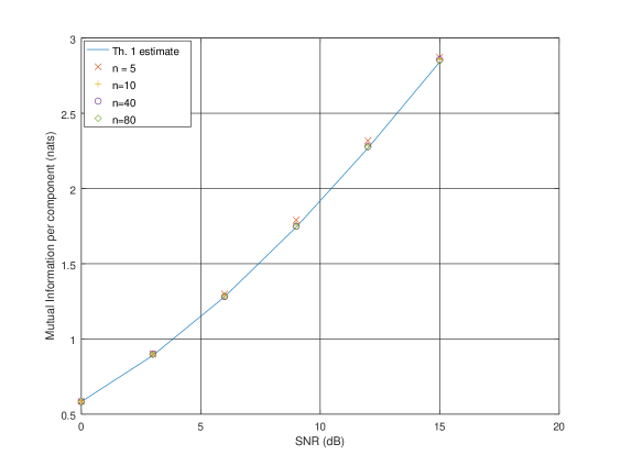
Figure 1: Plots of $\hat{\mathcal{I}}_{1,n}$ and $\hat{\mathcal{I}}_{4000}^{\mathrm{\,Th1}}$ w.r.t. the SNR and $n$. Setting: $R=T=2$, $L=3$, $f_{\text{d}}=0.05$. Each empirical average $\hat{\mathcal{I}}_{1,n}$ comes from $150$ channel realizations.

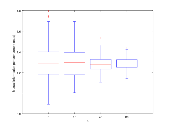
Figure 2: Boxplots of $\hat{\mathcal{I}}_{1,n}$ w.r.t. $n$. Same setting as for Fig. 1 with $\rho=6$ dB. The continuous horizontal line represents $\hat{\mathcal{I}}_{4000}^{\mathrm{\,Th1}}$.

Figure 1 shows that the estimates of $\mathcal{I}_{\rho}$ obtained by doing empirical averages ${\mathcal{I}}_{1,n}$ are not affected by important biases. However, Figure 2 shows that the dispersion parameters associated with these estimates are still important for $n$ as large as $80$. We note that in the setting of this figure, the matrix $H_{1,n}H_{1,n}^{*}\in\mathbb{C}^{nRL\times nRL}$ is a $480\times 480$ matrix when $n=80$. On the other hand, the mutual information estimates $\hat{\mathcal{I}}_{n}^{\mathrm{\,Th1}}$ provided by Theorem 1 require much less numerical computations since they involve the inversions of $RL\times RL=6\times 6$ matrices.

The large random matrix regime.

Next, we consider the asymptotic regime where both $N$ and $K$ converge to infinity at the same pace. For a large class of processes $({\mathsf{F}}_{n},{\mathsf{G}}_{n})$, it happens that in this regime, the Density of States of the operator ${\mathsf{H}}{\mathsf{H}}^{*}$ (which should now be indexed by $K,N$) converges to a probability measure encountered in the field of large random matrix theory; see [17] for “Wigner analogues” of our model, and [12] for models closer to those of this paper. One important feature of this probability measure is that it depends on the probability law of the channel process only through its first and second order statistics.

We illustrate herein this phenomenon on an instance of the MIMO frequency and time selective channel described at the beginning of this section. We observe that in this applicative setting, the regime of convergence of $N,K\to\infty$ at the same rate embeds the case where $R$ and $T$ are fixed while $L\to\infty$, the case where $L$ is fixed while $R,T\to\infty$ at the same pace, as well as the intermediate cases. For the simplicity of the presentation, we assume that the numbers of antennas $R$ and $T$ are equal (note that $N=K=RL$ in this case), and moreover, set the AR coefficient $\alpha=0$. If we let $N\to\infty$, we get the following result:

Proposition 5 (large dimensional regime).

Within the specific model described above, assume the vector $a$, which depends on $L$, satisfies $\|a\|=1$ for every $L$, and that

$$\sup_{L}\max_{\ell\in\{0,\ldots,L\}}\sqrt{L}|a_{\ell}|<\infty,$$ (36)

(which is trivially satisfied if $L$ is fixed). Then,

$$\lim_{N\to\infty}{\mathcal{I}}_{\rho}=2\log\frac{\sqrt{4\rho+1}+1}{2}-\frac{2\rho+1-\sqrt{4\rho+1}}{2\rho}\,.$$ (37)

To prove this proposition, we shall show that $\mathcal{I}_{\rho}$ converges as $N\to\infty$ to $\int\log(1+\rho\lambda)\,\mu_{\text{MP}}(d\lambda)$, where $\mu_{\text{MP}}(d\lambda)=(2\pi)^{-1}\sqrt{4/\lambda-1}\mathbbm{1}_{[0,4]}(\lambda)\,d\lambda$. This is the element of the family of the celebrated Marchenko-Pastur distributions which is the limiting spectral measure of $XX^{*}$ when $X$ is a square random matrix with iid elements. We provide a proof in Section 6 which is based on Theorem 1. More sophisticated channel models can be considered, including non centered models or models with correlations along the time index $n$, and for which one can prove similar asymptotics, see [12]. Note also that in the context of the large random matrix theory, a similar model where $L$ is fixed and $R,T\to\infty$ at the same rate has been considered in [24].

We illustrate this result on an example, represented in Figure 3. As an instance of the statistical channel model used in the statement of Proposition 5, we assume a generalized Wyner model as described in the introduction of this paper. We fix $R$ and $T$ to equal values, and we consider the regime where the network of Base Stations becomes denser and denser, making $L$ converge to infinity. By densifying the network, the number of users occupying a frequency slot will grow linearly with the number of BS. The number of interferers will grow as well. Yet, provided the BS are connected through a high rate backbone to a central processing unit which is able to perform a joint processing, the overall network capacity will grow linearly with $L$. To be more specific, we assume that the channel power gain when the mobile is at the distance $d$ to the BS is

$$\frac{1}{10+(10d/D)^{3}}\mathbbm{1}_{[-D/2,D/2]}(d),$$ (38)

where $D>0$ is a parameter that has the dimension of a distance. If the BS are regularly spaced, and if there are $L$ Base Stations per $D$ units of distance, then one channel model approaching this power decay behavior is the setting where the $a_{\ell}$’s are given by

$$a_{\ell}^{2}\propto\frac{1}{10+\left|10(\ell-L/2)/L\right|^{3}},\quad\ell\in\{0,\ldots,L\}.$$ (39)

The quantity $R\times\lim_{L\to\infty}\mathcal{I}_{\rho}$, where the limit is given by Proposition 5, thus represents the ergodic mutual information per user. Figure 3 shows that the predictions of Proposition 5 fit with the values provided by Theorem 1 for $L$ as small as one.

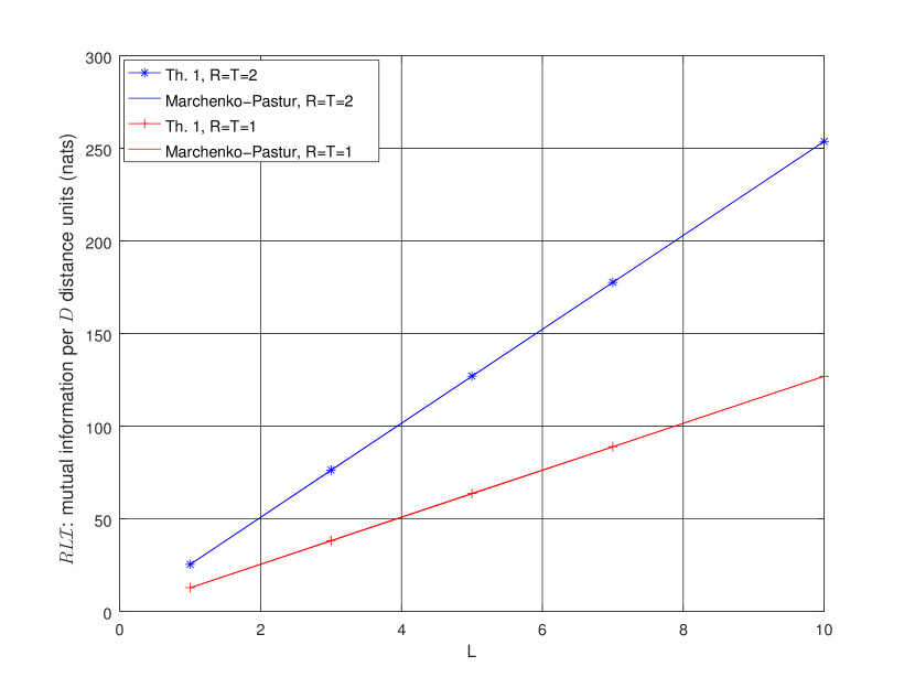
Figure 3: Aggregated mutual information vs density of the BS. Setting: $\rho=6\text{dB}$.

Illustration of Theorem 2.

Finally, we illustrate the asymptotic behavior of $\mathcal{I}_{\rho}$ in the high SNR regime as predicted by Theorem 2. In this experiment, we consider a more general model than the one described above where we replace the centered channel coefficient matrix $c_{n,\ell}$ of the model by

$$\sqrt{\frac{K_{\text{R}}}{K_{\text{R}}+1}}d_{n,\ell}+\sqrt{\frac{1}{K_{\text{R}}+1}}c_{n,\ell},$$ (40)

where $d_{n,\ell}:=[d_{n,\ell}(r,t)]_{r,t=0}^{R-1,T-1}$ is a determistic matrix with entries

$$d_{n,\ell}(r,t)=a_{\ell}\exp(2\imath\pi(r-t)\sin(\pi\ell/L)),$$ (41)

and where the nonnegative number $K_{\text{R}}$ plays the role of the so-called Rice factor. We take again $a_{\ell}\propto\exp(-0.4\ell)$ and $\alpha=\exp(-f_{\text{d}})$ as in the first paragraph of the section. The high SNR behavior of $\mathcal{I}_{\rho}$ is illustrated by Figure 4.

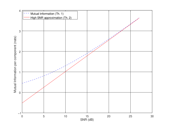
Figure 4: High SNR behavior of $\mathcal{I}_{\rho}$. Setting: $R=3$, $T=2$, $L=3$, $f_{\text{d}}=0.05$, $K_{\text{R}}=10$.

Keeping the same channel model, the behavior of $\kappa_{\infty}$ in terms of the Doppler frequency $f_{\text{d}}$ and the Rice factor is illustrated by Figure 5. This figure shows that the impact of $f_{\text{d}}$ is marginal. Regarding $K_{\text{R}}$, the channel randomness has a beneficial effect on the mutual information for our model, assuming of course that the channel is perfectly known at the receiver.

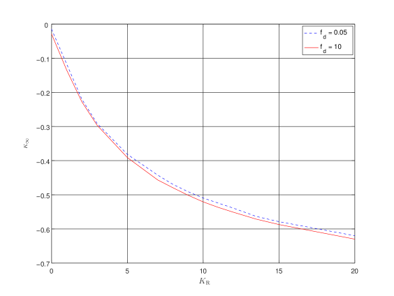
Figure 5: Behavior of $\kappa_{\infty}$ w.r.t. $f_{\text{d}}$ and $K_{\text{R}}$. Setting: $R=3$, $T=2$, $L=3$.

4 Proofs of Theorem 1

In this section, we let Assumption 1 hold true.

4.1 Preparation

The idea behind the proof of Theorem 1 is to show that $\mathcal{I}_{\rho}$ can be given an expression that involves the resolvents of infinite block-Jacobi matrices and to manipulate these resolvents to obtain the recursion formula for ${\mathsf{W}}_{n}$. We denote for any $m,n\in\mathbb{Z}\cup\{\pm\infty\}$ by ${\mathsf{H}}_{m,n}$ the operator on $\ell^{2}:=\ell^{2}(\mathbb{Z})$ defined as the truncation of ${\mathsf{H}}$, defined in (18), having the bi-infinite matrix representation

$${\mathsf{H}}_{m,n}=\begin{bmatrix}{\mathsf{F}}_{m}&{\mathsf{G}}_{m}\\ &{\mathsf{F}}_{m+1}&{\mathsf{G}}_{m+1}\\ &&\ddots&\ddots\\ &&&{\mathsf{F}}_{n}&{\mathsf{G}}_{n}\end{bmatrix}$$ (42)

where the remaining entries are set to zero. Recalling the definition of the random matrix ${\mathsf{H}}_{m,n}$ already provided in (10) for finite $m,n\in\mathbb{Z}$, we thus identify this matrix with the associated finite rank operator acting on $\ell^{2}$ for which we use the same notation.

Let us now introduce a convenient notation: If one considers an operator on $\ell^{2}$ with block-matrix form $\mathsf{A}=\big{[}\mathsf{A}_{ij}\big{]}_{i,j\in\mathbb{Z}},$ where the $\mathsf{A}_{ij}$’s are $Q\times Q$ matrices, then $[\mathsf{A}]_{\Box_{Q}}$ stands for the $Q\times Q$ block $\mathsf{A}_{ii}$ with largest index $i\in\mathbb{Z}$ such that $\mathsf{A}_{ii}\neq 0$. For the operators of interest in this work, $[\mathsf{A}]_{\Box_{Q}}$ will always be the bottom rightmost non-vanishing $Q\times Q$ block. Of importance in the proof will be the operators of the type ${\mathsf{H}}_{-\infty,n}$. This operator is closed and densely defined, thus, defining as ${\mathsf{H}}_{-\infty,n}^{*}$ is adjoint, the operator ${\mathsf{H}}_{-\infty,n}^{*}{\mathsf{H}}_{-\infty,n}$ is a positive self-adjoint operator [12, Sec. 4],[1, Sec. 46]. Thus, the resolvent $(I+\rho\,{\mathsf{H}}_{-\infty,n}^{*}{\mathsf{H}}_{-\infty,n})^{-1}$ is defined for each $\rho>0$, and we can set

$${\mathsf{W}}_{n}:=[(I+\rho\,{\mathsf{H}}_{-\infty,n}^{*}{\mathsf{H}}_{-\infty,n})^{-1}]_{\Box_{K}}.$$ (43)

We shall prove that the sequence $({\mathsf{W}}_{n})$ indeed satisfies the statements of Theorem 1. To do so, we will use in a key fashion the following Schur complement identities:

$$\det\begin{bmatrix}A&B\\ C&D\end{bmatrix} =\det D\times\det(A-BD^{-1}C)\,,$$ (44)

$$\begin{bmatrix}A&B\\ C&D\end{bmatrix}^{-1} =\begin{bmatrix}(A-BD^{-1}C)^{-1}&\times\\ \times&(D-CA^{-1}B)^{-1}\end{bmatrix}\,,$$ (45)

where the $\times$’s can be made explicit in terms of $A,B,C,D$ but are not of interest for our purpose.

4.2 Proof of Theorem 1(a)

We first show that ${\mathsf{W}}_{n}$ defined in (43) indeed satisfies the recursive equations (12), that is we prove the existence part of Theorem 1(a).

4.2.1 Existence

Proof of Theorem 1(a); existence.

Introduce the truncation of ${\mathsf{H}}_{-\infty,n}$ defined by deleting the rightmost non-zero column,

$$\widetilde{\mathsf{H}}_{-\infty,n}:=\begin{bmatrix}\ddots&\ddots\\ &{\mathsf{F}}_{n-1}&{\mathsf{G}}_{n-1}\\ &&{\mathsf{F}}_{n}\end{bmatrix}\,,$$ (46)

so that

$${\mathsf{H}}_{-\infty,n}=\left[\begin{array}[]{c|c}\widetilde{\mathsf{H}}_{-\infty,n}&\begin{array}[]{c}0\\ {\mathsf{G}}_{n}\end{array}\end{array}\right]=:\left[\begin{array}[]{c|c}\widetilde{\mathsf{H}}_{-\infty,n}&Q\end{array}\right].$$ (47)

Recalling ${\mathsf{W}}_{n}$’s definition (43), the Schur’s complement formula (45) then provides

$${\mathsf{W}}_{n} =\left(\begin{bmatrix}I+\rho\,\widetilde{\mathsf{H}}_{-\infty,n}^{*}\widetilde{\mathsf{H}}_{-\infty,n}&\rho\,\widetilde{\mathsf{H}}_{-\infty,n}^{*}Q\\ \rho\,Q^{*}\widetilde{\mathsf{H}}_{-\infty,n}&I+\rho\,{\mathsf{G}}_{n}^{*}{\mathsf{G}}_{n}\end{bmatrix}^{-1}\right)_{\Box_{K}}$$

$$\stackrel{{\scriptstyle(a)}}{{=}}\left(I+\rho\,{\mathsf{G}}_{n}^{*}{\mathsf{G}}_{n}-\rho^{2}\,Q^{*}\widetilde{\mathsf{H}}_{-\infty,n}(I+\rho\,\widetilde{\mathsf{H}}_{-\infty,n}^{*}\widetilde{\mathsf{H}}_{-\infty,n})^{-1}\widetilde{\mathsf{H}}_{-\infty,n}^{*}Q\right)^{-1}$$

$$\stackrel{{\scriptstyle(b)}}{{=}}\left(I+\rho\,{\mathsf{G}}_{n}^{*}\widetilde{\mathsf{W}}_{n}{\mathsf{G}}_{n}\right)^{-1}$$ (48)

where we introduced

$$\widetilde{\mathsf{W}}_{n}:=[(I+\rho\,\widetilde{\mathsf{H}}_{-\infty,n}^{*}\widetilde{\mathsf{H}}_{-\infty,n})^{-1}]_{\Box_{N}}.$$ (49)

Here the identity $\stackrel{{\scriptstyle(a)}}{{=}}$ can be easily checked similarly to its finite dimensional counterpart, and $\stackrel{{\scriptstyle(b)}}{{=}}$ is shown in, e.g., [12, Lemma 7.2].

By similarly expressing $\widetilde{\mathsf{H}}_{-\infty,n}$ in terms of ${\mathsf{H}}_{-\infty,n-1}$ and ${\mathsf{F}}_{n}$, the same computation further yields

$$\widetilde{\mathsf{W}}_{n}=\left(I+\rho\,{\mathsf{F}}_{n}{\mathsf{W}}_{n-1}{\mathsf{F}}_{n}^{*}\right)^{-1}$$ (50)

and thus we obtain with (48) the identity

$${\mathsf{W}}_{n}=\left(I+\rho\,{\mathsf{G}}_{n}^{*}\left(I+\rho\,{\mathsf{F}}_{n}{\mathsf{W}}_{n-1}{\mathsf{F}}_{n}^{*}\right)^{-1}{\mathsf{G}}_{n}\right)^{-1}.$$ (51)

∎

4.2.2 Uniqueness

Next, we establish the uniqueness of the process $({\mathsf{W}}_{n})_{n\in\mathbb{Z}}$ satisfying the recursive relations (12) within the class of stationary processes, to complete the proof of Theorem 1(a).

The proof relies on a contraction argument with the distance on ${\mathcal{H}}_{m}^{++}$ for $m$ being a positive integer:

$$\mathrm{dist}:{\mathcal{H}}_{m}^{++}\times{\mathcal{H}}_{m}^{++}\to[0,\infty),\quad(X,Y)\mapsto\left[\mathrm{Tr}\log^{2}(XY^{-1})\right]^{1/2}\,,$$ (52)

which is the geodesic distance associated with the Riemannian metric $g_{X}(A,B):=\mathrm{Tr}(X^{-1}AX^{-1}B)$ on the convex cone ${\mathcal{H}}_{m}^{++}$; we refer e.g. to [5, §1.2] or [21, §3] for further information. Convergence in $\mathrm{dist}$ is equivalent to convergence in the Euclidean norm. It has the following invariance properties: for any $X,Y\in{\mathcal{H}}_{m}^{++}$ and any $m\times m$ complex invertible matrix $A$,

$$\mathrm{dist}(X,Y)=\mathrm{dist}(AXA^{*},AYA^{*}),\qquad\mathrm{dist}(X,Y)=\mathrm{dist}(X^{-1},Y^{-1})\,.$$ (53)

Moreover, for any $S\in{\mathcal{H}}_{m}^{+}$, we have according to [5, Prop. 1.6],

$$\mathrm{dist}(X+S,Y+S)\leq\frac{\max(\|X\|,\|Y\|)}{\max(\|X\|,\|Y\|)+{\lambda_{\text{min}}}(S)}\,\mathrm{dist}(X,Y)\,,$$ (54)

where ${\lambda_{\text{min}}}(S)$ is the smallest eigenvalue of $S$. We also have the following result, which will be the key to prove the uniqueness of the process:

Lemma 6.

Given two positive integers $k$ and $n$ such that $n\geq k$, let $X,Y\in{\mathcal{H}}_{k}^{++}$, $S\in{\mathcal{H}}_{n}^{++}$, and $A\in\mathbb{C}^{n\times k}$. Then,

$$\mathrm{dist}(AXA^{*}+S,AYA^{*}+S)\leq\frac{\max(\|AXA^{*}\|,\|AYA^{*}\|)}{\max(\|AXA^{*}\|,\|AYA^{*}\|)+{\lambda_{\text{min}}}(S)}\,\mathrm{dist}(X,Y)\,.$$ (55)

Proof.

Define in ${\mathcal{H}}_{n}^{++}$ the two matrices

$$X^{\prime}=\begin{bmatrix}X\\ &I_{n-k}\end{bmatrix}\quad\text{and}\quad Y^{\prime}=\begin{bmatrix}Y\\ &I_{n-k}\end{bmatrix}.$$ (56)

Let $(B_{\ell})$ be a sequence of matrices in $\mathbb{C}^{n\times n}$ such that $B_{\ell}$ is invertible for each $\ell\in{{\mathbb{N}}}$, and such that $B_{\ell}\to\begin{bmatrix}A&0\end{bmatrix}$ as $\ell\to\infty$ (such a sequence is guaranteed to exist by the density of the set of invertible matrices in $\mathbb{C}^{n\times n}$). Using the first identity in (53) and Inequality (54), and observing that $\mathrm{dist}(X,Y)=\mathrm{dist}(X^{\prime},Y^{\prime})$, we get that

$$\mathrm{dist}(B_{\ell}X^{\prime}B_{\ell}^{*}+S,B_{\ell}Y^{\prime}B_{\ell}^{*}+S)\leq\frac{\max(\|B_{\ell}X^{\prime}B_{\ell}^{*}\|,\|B_{\ell}Y^{\prime}B_{\ell}^{*}\|)}{\max(\|B_{\ell}X^{\prime}B_{\ell}^{*}\|,\|B_{\ell}Y^{\prime}B_{\ell}^{*}\|)+{\lambda_{\text{min}}}(S)}\mathrm{dist}(X,Y).$$ (57)

Making $\ell\to\infty$, and recalling that the geodesic and the Euclidean topologies are equivalent, we obtain the result. ∎

Proof of Theorem 1(a); uniqueness.

To prove the uniqueness, we assume that $N\geq K$ for simplicity, since the case $N<K$ can be treated in a similar manner. If one introduces, for any $F,G\in\mathbb{C}^{N\times K}$, the mapping $\psi_{F,G}:{\mathcal{H}}_{K}^{++}\to{\mathcal{H}}_{K}^{++}$ defined by

$$\psi_{F,G}(W):=\left(I+\rho\,G^{*}\left(I+\rho\,FWF^{*}\right)^{-1}G\right)^{-1},$$ (58)

then (12) reads ${\mathsf{W}}_{n}=\psi_{{\mathsf{F}}_{n},{\mathsf{G}}_{n}}({\mathsf{W}}_{n-1})$. This mapping can be written as

$$\psi_{F,G}(W)=\iota\circ\tau_{\sqrt{\rho}G^{*};I}\circ\iota\circ\tau_{\sqrt{\rho}F;I}(W),$$ (59)

where we set

$$\tau_{A;S}(X):=AXA^{*}+S\quad\text{and}\quad\iota(X):=X^{-1}\,$$ (60)

with a small notational abuse related to the fact that, e.g., the two functions $\iota$ used in (59) are not the same in general. Using Lemma 6 together with the invariance of $\mathrm{dist}$ with respect to the inversion, we obtain for any $W,W^{\prime}\in{\mathcal{H}}_{K}^{++}$,

$$\mathrm{dist}\big{(}\psi_{F,G}(W),\psi_{F,G}(W^{\prime})\big{)}$$

$$\leq\frac{\rho\|G\|^{2}}{\rho\|G\|^{2}+1}\frac{\max(\|\rho FWF^{*}\|,\|\rho FW^{\prime}F^{*}\|)}{\max(\|\rho FWF^{*}\|,\|\rho FW^{\prime}F^{*}\|)+1}\,\mathrm{dist}(W,W^{\prime})$$

$$\leq\frac{\rho\|G\|^{2}}{\rho\|G\|^{2}+1}\,\mathrm{dist}(W,W^{\prime}),$$ (61)

where for the first inequality we used that $\|G^{*}(I+\rho FWF^{*})^{-1}G\|\leq\|G\|^{2}$ for any $W\in{\mathcal{H}}_{K}^{+}$, and that the function $x\mapsto x/(x+1)$ is increasing.

Now, let $({\mathsf{W}}_{n}^{\prime})_{n\in\mathbb{Z}}$ be any stationary process on ${\mathcal{H}}_{K}^{++}$ satisfying ${\mathsf{W}}_{n}^{\prime}=\psi_{{\mathsf{F}}_{n},{\mathsf{G}}_{n}}({\mathsf{W}}_{n-1}^{\prime})$ a.s. for every $n\in\mathbb{Z}$. If we let $n\geq 0$, then we have from (4.2.2) a.s. that

$$\mathrm{dist}({\mathsf{W}}_{n},{\mathsf{W}}^{\prime}_{n})\leq\frac{\rho\|{\mathsf{G}}_{n}\|^{2}}{\rho\|{\mathsf{G}}_{n}\|^{2}+1}\mathrm{dist}({\mathsf{W}}_{n-1},{\mathsf{W}}^{\prime}_{n-1})$$ (62)

and, iterating, we obtain

$$\mathrm{dist}({\mathsf{W}}_{n},{\mathsf{W}}^{\prime}_{n})\leq\Bigl{(}\prod_{i=1}^{n}\xi_{i}\Bigr{)}\,\mathrm{dist}({\mathsf{W}}_{0},{\mathsf{W}}^{\prime}_{0}),\qquad\xi_{i}:=\frac{\rho\|{\mathsf{G}}_{i}\|^{2}}{\rho\|{\mathsf{G}}_{i}\|^{2}+1}.$$ (63)

By the ergodicity of $({\mathsf{G}}_{n})_{n\in\mathbb{Z}}$, we have

$$\frac{1}{n}\sum_{i=1}^{n}\log\xi_{i}\xrightarrow[n\to\infty]{\text{a.s.}}{{\mathbb{E}}}\log\xi_{0}<0$$ (64)

and thus we have proven that $\mathrm{dist}({\mathsf{W}}_{n},{\mathsf{W}}^{\prime}_{n})\to 0$ a.s. as $n\to\infty$. Finally, since

$$({\mathsf{W}}_{n+m_{1}},\ldots,{\mathsf{W}}_{n+m_{M}})\stackrel{{\scriptstyle\text{law}}}{{=}}({\mathsf{W}}_{m_{1}},\ldots,{\mathsf{W}}_{m_{M}})$$ (65)

for any $M-$tuple of integers $(m_{1},\ldots,m_{M})$ and similarly for ${\mathsf{W}}_{n}^{\prime}$, by letting $n\to\infty$ this yields that the finite-dimensional distributions of the two stationary processes $({\mathsf{W}}_{n})_{n\in\mathbb{Z}}$ and $({\mathsf{W}}^{\prime}_{n})_{n\in\mathbb{Z}}$ are the same, and consequently these two processes have the same distribution. ∎

4.3 Proof of Theorem 1(b)

We start with the following lemma.

Lemma 7.

For any fixed $n\in\mathbb{Z}$ and $\rho>0$, we have

$$[(I+\rho\,{\mathsf{H}}_{m,n}^{*}{\mathsf{H}}_{m,n})^{-1}]_{\Box_{K}}\xrightarrow[m\to-\infty]{}{\mathsf{W}}_{n}.$$ (66)

Proof.

Denote by ${\mathcal{K}}\subset\ell^{2}$ the subspace of sequences with finite support. Clearly, for any fixed $n\in\mathbb{Z}$ and fixed event $\omega\in\Omega$, we have for all $x\in{\mathcal{K}}$,

$${\mathsf{H}}_{m,n}^{*}{\mathsf{H}}_{m,n}x\xrightarrow[m\to-\infty]{}{\mathsf{H}}_{-\infty,n}^{*}{\mathsf{H}}_{-\infty,n}x\,,$$ (67)

where $\to$ denotes the strong convergence in $\ell^{2}$. Now ${\mathcal{K}}$ is a common core for the set of operators $\{{\mathsf{H}}_{m,n}^{*}{\mathsf{H}}_{m,n}:m\in\{n,n-1,n-2,\ldots\}\}$ and ${\mathsf{H}}_{-\infty,n}^{*}{\mathsf{H}}_{-\infty,n}$, see e.g. [16, §III.5.3] or [27, Chap. VIII] for this notion. As a consequence, the convergence also holds in the strong resolvent sense, see [27, §VIII], and thus for every $x\in\ell^{2}$ and $\rho>0$,

$$(I+\rho\,{\mathsf{H}}_{m,n}^{*}{\mathsf{H}}_{m,n})^{-1}x\xrightarrow[n\to\infty]{}(I+\rho\,{\mathsf{H}}_{-\infty,n}^{*}{\mathsf{H}}_{-\infty,n})^{-1}x\quad\text{ a.s.}$$ (68)

from which (66) follows by definition (43) of ${\mathsf{W}}_{n}$. ∎

Proof of Theorem 1(b).

We start by writing

$${\mathsf{H}}_{m,n}=\left[\begin{array}[]{c}\begin{array}[]{c|c}{\mathsf{H}}_{m,n-1}&0\\ \hline\cr\begin{matrix}0&\cdots&0&{\mathsf{F}}_{n}\end{matrix}&{\mathsf{G}}_{n}\end{array}\end{array}\right]=\left[\begin{array}[]{c}\begin{array}[]{c|c}{\mathsf{H}}_{m,n-1}&0\\ \hline\cr P&{\mathsf{G}}_{n}\end{array}\end{array}\right]$$ (69)

with $P:=[\ 0\ \cdots\ 0\ {\mathsf{F}}_{n}]$, and use Schur’s complement formula (44) to obtain,

$$\log\det(I+\rho\,{\mathsf{H}}_{m,n}{\mathsf{H}}_{m,n}^{*})$$

$$=\log\det\begin{bmatrix}I+\rho\,{\mathsf{H}}_{m,n-1}{\mathsf{H}}_{m,n-1}^{*}&\rho\,{\mathsf{H}}_{n,m-1}^{*}P^{*}\\ \rho\,P{\mathsf{H}}_{m,n-1}^{*}&I+\rho\,{\mathsf{F}}_{n}{\mathsf{F}}_{n}^{*}+\rho\,{\mathsf{G}}_{n}{\mathsf{G}}_{n}^{*}\end{bmatrix}$$

$$=\log\det(I+\rho\,{\mathsf{H}}_{m,n-1}{\mathsf{H}}_{m,n-1}^{*})$$

$$\phantom{=}+\log\det\left(I+\rho\,{\mathsf{F}}_{n}{\mathsf{F}}_{n}^{*}+\rho\,{\mathsf{G}}_{n}{\mathsf{G}}_{n}^{*}-\rho^{2}\,P{\mathsf{H}}_{m,n-1}^{*}(I+\rho\,{\mathsf{H}}_{m,n-1}{\mathsf{H}}_{m,n-1}^{*})^{-1}{\mathsf{H}}_{n,m-1}P^{*}\right)$$

$$=\log\det(I+\rho\,{\mathsf{H}}_{m,n-1}{\mathsf{H}}_{m,n-1}^{*})$$

$$\phantom{=}+\log\det\left(I+\rho\,{\mathsf{F}}_{n}{\mathsf{F}}_{n}^{*}+\rho\,{\mathsf{G}}_{n}{\mathsf{G}}_{n}^{*}+\rho\,P[(I+\rho\,{\mathsf{H}}_{m,n-1}^{*}{\mathsf{H}}_{m,n-1})^{-1}-I]P^{*}\right)$$

$$=\log\det(I+\rho\,{\mathsf{H}}_{m,n-1}{\mathsf{H}}_{m,n-1}^{*})$$

$$\phantom{=}+\log\det\left(I+\rho\,{\mathsf{F}}_{n}{\mathsf{F}}_{n}^{*}+\rho\,{\mathsf{G}}_{n}{\mathsf{G}}_{n}^{*}+\rho\,{\mathsf{F}}_{n}[(I+\rho\,{\mathsf{H}}_{m,n-1}^{*}{\mathsf{H}}_{m,n-1})^{-1}-I]_{\Box K}{\mathsf{F}}_{n}^{*}\right)$$

$$=\log\det(I+\rho\,{\mathsf{H}}_{m,n-1}{\mathsf{H}}_{m,n-1}^{*})$$

$$\phantom{=}+\log\det\left(I+\rho\,{\mathsf{G}}_{n}{\mathsf{G}}_{n}^{*}+\rho\,{\mathsf{F}}_{n}[(I+\rho\,{\mathsf{H}}_{m,n-1}^{*}{\mathsf{H}}_{m,n-1})^{-1}]_{\Box_{K}}{\mathsf{F}}_{n}^{*}\right).$$ (70)

By iterating this manipulation after replacing ${\mathsf{H}}_{m,n-i}$ by ${\mathsf{H}}_{m,n-i-1}$ at the $i^{\text{th}}$ step, if we set

$$\xi_{m,i}:=\log\det\left(I+\rho\,{\mathsf{G}}_{i}{\mathsf{G}}_{i}^{*}+\rho\,{\mathsf{F}}_{i}[(I+\rho\,{\mathsf{H}}_{m,i-1}^{*}{\mathsf{H}}_{m,i-1})^{-1}]_{\Box_{K}}{\mathsf{F}}_{i}^{*}\right)$$ (71)

for any $m\leq i\leq n$ with the convention that ${\mathsf{H}}_{m,m-1}:=0$, we have

$$\log\det\left(I+\rho\,{\mathsf{H}}_{m,n}{\mathsf{H}}_{m,n}^{*}\right)=\sum_{i=m}^{n}\xi_{m,i}\,.$$ (72)

Next, Lemma 7 yields

$$\xi_{m,i}\xrightarrow[m\to-\infty]{}\log\det\left(I+\rho\,{\mathsf{G}}_{i}{\mathsf{G}}_{i}^{*}+\rho\,{\mathsf{F}}_{i}{\mathsf{W}}_{i-1}{\mathsf{F}}_{i}^{*}\right).$$ (73)

Since $\|[(I+\rho\,{\mathsf{H}}_{m,i-1}^{*}{\mathsf{H}}_{m,i-1})^{-1}]_{\Box_{K}}\|\leq 1$, we have $\xi_{m,i}\leq N\log(1+\rho\|{\mathsf{F}}_{i}\|^{2}+\rho\|{\mathsf{G}}_{i}\|^{2})$. Thus, by the moment assumption (6), we obtain from (73) and dominated convergence that

$${{\mathbb{E}}}\xi_{m,i}\xrightarrow[m\to-\infty]{} \,{{\mathbb{E}}}\log\det\left(I+\rho\,{\mathsf{G}}_{i}{\mathsf{G}}_{i}^{*}+\rho\,{\mathsf{F}}_{i}{\mathsf{W}}_{i-1}{\mathsf{F}}_{i}^{*}\right)$$

$$={{\mathbb{E}}}\log\det\left(I+\rho\,{\mathsf{G}}_{0}{\mathsf{G}}_{0}^{*}+\rho\,{\mathsf{F}}_{0}{\mathsf{W}}_{-1}{\mathsf{F}}_{0}^{*}\right),$$ (74)

where the equality follows from the stationarity of the process $({\mathsf{F}}_{n},{\mathsf{G}}_{n})_{n\in\mathbb{Z}}$. The stationarity further provides that ${{\mathbb{E}}}\xi_{m,i}$ only depends on $i-m$ and thus, for any fixed $n$, we obtain by Cesàro summation (see [26, Page 16]) that

$$N\mathcal{I}_{\rho}=\lim_{m\to-\infty}\frac{1}{(n-m+1)}\sum_{i=m}^{n}{{\mathbb{E}}}\xi_{m,i}={{\mathbb{E}}}\log\det\left(I+\rho\,{\mathsf{G}}_{0}{\mathsf{G}}_{0}^{*}+\rho\,{\mathsf{F}}_{0}{\mathsf{W}}_{-1}{\mathsf{F}}_{0}^{*}\right).$$ (75)

By taking $n=0$ in the recursive relation (12), we moreover see that

$$N\mathcal{I}_{\rho} ={{\mathbb{E}}}\log\det\left(I+\rho\,{\mathsf{G}}_{0}{\mathsf{G}}_{0}^{*}+\rho\,{\mathsf{F}}_{0}{\mathsf{W}}_{-1}{\mathsf{F}}_{0}^{*}\right)$$

$$={{\mathbb{E}}}\log\det\left(I+\rho\,{\mathsf{F}}_{0}{\mathsf{W}}_{-1}{\mathsf{F}}_{0}^{*}\right)+{{\mathbb{E}}}\log\det\left(I+\rho\,{\mathsf{G}}_{0}{\mathsf{G}}_{0}^{*}(I+\rho\,{\mathsf{F}}_{0}{\mathsf{W}}_{-1}{\mathsf{F}}_{0}^{*})^{-1}\right)$$

$$={{\mathbb{E}}}\log\det\left(I+\rho\,{\mathsf{F}}_{0}{\mathsf{W}}_{-1}{\mathsf{F}}_{0}^{*}\right)+{{\mathbb{E}}}\log\det\left(I+\rho\,{\mathsf{G}}_{0}^{*}(I+\rho\,{\mathsf{F}}_{0}{\mathsf{W}}_{-1}{\mathsf{F}}_{0}^{*})^{-1}{\mathsf{G}}_{0}\right)$$

$$={{\mathbb{E}}}\log\det\left(I+\rho\,{\mathsf{F}}_{0}{\mathsf{W}}_{-1}{\mathsf{F}}_{0}^{*}\right)-{{\mathbb{E}}}\log\det{\mathsf{W}}_{0},$$ (76)

which proves (13). ∎

4.4 Proof of Theorem 1(c)

Proof of Theorem 1(c).

Since the process $({\mathsf{F}}_{n},{\mathsf{G}}_{n})_{n\in\mathbb{Z}}$ is assumed to be ergodic, and so does $({\mathsf{W}}_{n})_{n\in\mathbb{Z}}$ by construction, we have a.s.

$$\lim_{n\to\infty}\frac{1}{n}\sum_{\ell=0}^{n-1}\log\det\left(I+\rho\,{\mathsf{F}}_{\ell}{\mathsf{W}}_{\ell-1}{\mathsf{F}}_{\ell}^{*}\right)-{{\mathbb{E}}}\log\det{\mathsf{W}}_{\ell}\\ ={{\mathbb{E}}}\log\det\left(I+\rho\,{\mathsf{F}}_{0}{\mathsf{W}}_{-1}{\mathsf{F}}_{0}^{*}\right)-{{\mathbb{E}}}\log\det{\mathsf{W}}_{0}=\mathcal{I}_{\rho}.$$ (77)

Next, for the same reason as and with the same notations as in the proof of the uniqueness of ${\mathsf{W}}_{n}$ provided in Section 4.2.2, we have $\mathrm{dist}({\mathsf{X}}_{n},{\mathsf{W}}_{n})\to 0$ a.s. as $n\to\infty$. Thus,

$$\frac{1}{n}\sum_{\ell=0}^{n-1}\log\det{\mathsf{X}}_{\ell}-\log\det{\mathsf{W}}_{\ell}\xrightarrow[n\to\infty]{\text{a.s.}}0$$ (78)

as a Cesàro average. Since Lemma 6 also yields

$$\mathrm{dist}(I+\rho\,{\mathsf{F}}_{n}{\mathsf{X}}_{n-1}{\mathsf{F}}_{n}\,,\,I+\rho\,{\mathsf{F}}_{n}{\mathsf{W}}_{n-1}{\mathsf{F}}_{n})\leq\mathrm{dist}({\mathsf{X}}_{n-1},{\mathsf{W}}_{n-1})\xrightarrow[n\to\infty]{\text{a.s.}}0,$$ (79)

we similarly have

$$\frac{1}{n}\sum_{\ell=0}^{n-1}\log\det(I+\rho\,{\mathsf{F}}_{\ell}{\mathsf{X}}_{\ell-1}{\mathsf{F}}_{\ell}^{*})-\log\det(I+\rho\,{\mathsf{F}}_{\ell}{\mathsf{W}}_{\ell-1}{\mathsf{F}}_{\ell}^{*})\xrightarrow[n\to\infty]{\text{a.s.}}0.$$ (80)

and the result follows from this convergence along with (77). ∎

This completes the proof of Theorem 1.

5 Proof of Theorem 2

Assume from now that $N>K$ and that Assumption 2 holds true.

5.1 Preparation

To obtain an expansion of the type $\mathcal{I}_{\rho}=(K/N)\log\rho+\kappa_{\infty}+o(1)$ as $\rho\to\infty$, it is more convenient to work with the new variables:

$$\gamma:=\frac{1}{\rho}\in(0,\infty)\,,\qquad{\mathsf{Z}}_{\gamma,n}:=\gamma\,{\mathsf{W}}_{n}^{-1}\,.$$ (81)

Indeed, it follows the identity (13) of Theorem 1 and the stationarity of $({\mathsf{W}}_{n})_{n\in\mathbb{Z}}$ that

$$N\mathcal{I}_{\rho} =-{{\mathbb{E}}}\log\det{\mathsf{W}}_{0}+{{\mathbb{E}}}\log\det(I+\rho\,{\mathsf{F}}_{1}{\mathsf{W}}_{n}{\mathsf{F}}_{1}^{*})$$

$$=K\log\rho+{{\mathbb{E}}}\log\det{\mathsf{Z}}_{\gamma,0}+{{\mathbb{E}}}\log\det(I+{\mathsf{F}}_{1}{\mathsf{Z}}_{\gamma,0}^{-1}{\mathsf{F}}_{1}^{*})$$

$$=K\log\rho+{{\mathbb{E}}}\log\det{\mathsf{Z}}_{\gamma,0}+{{\mathbb{E}}}\log\det(I+{\mathsf{Z}}_{\gamma,0}^{-1}{\mathsf{F}}_{1}^{*}{\mathsf{F}}_{1})$$

$$=K\log\rho+{{\mathbb{E}}}\log\det({\mathsf{Z}}_{\gamma,0}+{\mathsf{F}}_{1}^{*}{\mathsf{F}}_{1}),$$ (82)

which is the starting point of the asymptotic analysis $\gamma\to 0$. With this expression at hand, we would like to take the limit $\gamma\to 0$ and identify the limit

$$\kappa_{\infty}:=\frac{1}{N}\lim_{\gamma\to 0}{{\mathbb{E}}}\log\det({\mathsf{Z}}_{\gamma,0}+{\mathsf{F}}_{1}^{*}{\mathsf{F}}_{1}).$$ (83)

To study this limiting case, we start from the recursive equation (12), which reads for these new variables

$${\mathsf{Z}}_{\gamma,n}=\gamma I+{\mathsf{G}}_{n}^{*}(I+{\mathsf{F}}_{n}{\mathsf{Z}}_{\gamma,n-1}^{-1}{\mathsf{F}}_{n}^{*})^{-1}{\mathsf{G}}_{n}=h_{\gamma,{\mathsf{F}}_{n},{\mathsf{G}}_{n}}({\mathsf{Z}}_{\gamma,n-1}),$$ (84)

where, for any $\gamma\geq 0$ and $F,G\in\mathbb{C}^{N\times K}$, we define $h_{\gamma,F,G}:{\mathcal{H}}_{K}^{++}\to{\mathcal{H}}_{K}^{+}$ by

$$h_{\gamma,F,G}(Z):=\gamma I+G^{*}(I+FZ^{-1}F^{*})^{-1}G\,.$$ (85)

Note that if $\gamma>0$ then $h_{\gamma,F,G}(Z)\in{\mathcal{H}}_{K}^{++}$. The same holds true when $\gamma=0$, which is now allowed, as soon as $G$ has full rank. We now observe that one can extend this mapping to the whole of ${\mathcal{H}}_{K}^{+}$.

5.1.1 Extension of the mapping $h_{\gamma,F,G}$ to ${\mathcal{H}}_{K}^{+}$

Assume that $F\in\mathbb{C}^{N\times K}$ has full rank, namely $\operatorname{rank}(F)=K$. By setting $T:=(F^{*}F)^{1/2}$ and $U:=F(F^{*}F)^{-1/2}$, we have the polar decomposition $F=UT$ where $U\in\mathbb{C}^{N\times K}$ is an isometry matrix and $T\in{\mathcal{H}}_{K}^{++}$. By completing $U$ so as to obtain a $N\times N$ unitary matrix $\begin{bmatrix}U\ \ U^{\perp}\end{bmatrix}$ and setting $\Pi_{F}^{\perp}:=U^{\perp}(U^{\perp})^{*}=I-F(F^{*}F)^{-1}F^{*}$, which the orthogonal projection onto the orthogonal space to the linear span of the columns of $F$, we can write

$$h_{\gamma,F,G}(Z)$$

$$=\gamma I+G^{*}(I+FZ^{-1}F^{*})^{-1}G$$

$$=\gamma I+G^{*}U(I+TZ^{-1}T)^{-1}U^{*}G+G^{*}\Pi_{F}^{\perp}G$$ (86)

$$=\gamma I+G^{*}UT^{-1}Z^{1/2}(I+Z^{1/2}T^{-2}Z^{1/2})^{-1}Z^{1/2}T^{-1}U^{*}G+G^{*}\Pi_{F}^{\perp}G$$

$$=\gamma I+G^{*}F(F^{*}F)^{-1}Z^{1/2}(I+Z^{1/2}(F^{*}F)^{-1}Z^{1/2})^{-1}Z^{1/2}(F^{*}F)^{-1}F^{*}G+G^{*}\Pi_{F}^{\perp}G$$ (87)

where for the second equality we used the matrix identity $(I+AB)^{-1}=B^{-1}(I+A^{-1}B^{-1})^{-1}A^{-1}$ with $A:=TZ^{-1/2}$ and $B:=Z^{-1/2}T$ for any $Z^{1/2}\in{\mathcal{H}}_{K}^{+}$ satisfying $(Z^{1/2})^{2}=Z$. Note that the alternative expression (87) for $h_{\gamma,F,G}(Z)$ does now make sense when $Z\in{\mathcal{H}}_{K}^{+}$ is not invertible, provided that $F$ has full rank. Moreover, since two Hermitian square roots of $Z\in{\mathcal{H}}_{K}^{+}$ are identical up to the multiplication by a unitary matrix, the right hand side of (87) does not depend on the choice for $Z^{1/2}$. In the following, we chose $Z\mapsto Z^{1/2}$ so that it is continuous (for the operator norm). Thus, by taking the right hand side of (87) as the definition of $h_{\gamma,F,G}(Z)$ in this case, we properly extended $h_{\gamma,F,G}$ to a mapping ${\mathcal{H}}_{K}^{+}\to{\mathcal{H}}_{K}^{+}$ which is continuous, and that we continue to denote by $h_{\gamma,F,G}$. An important property of $h_{0,F,G}$ we use in what follows is:

Lemma 8.

If $F$ has full rank, then $h_{0,F,G}:{\mathcal{H}}_{K}^{+}\to{\mathcal{H}}_{K}^{+}$ is non-decreasing.

Proof.

It is clear from (85) this mapping is non-decreasing on ${\mathcal{H}}_{K}^{++}$ and this property extends to ${\mathcal{H}}_{K}^{+}$ since one can write $h_{0,F,G}(Z)=\lim_{\varepsilon\to 0}h_{0,F,G}(Z+\varepsilon I)$ by continuity of $h_{0,F,G}$. ∎

5.1.2 The Markov kernel $Q_{\gamma}$

Equipped with the extended definition of $h_{\gamma,F,G}$ to ${\mathcal{H}}_{K}^{+}$, let us consider for any $\gamma\geq 0$ the Markov transition kernel $Q_{\gamma}:(E\times{\mathcal{H}}_{K}^{+})\times{\mathscr{B}}(E\times{\mathcal{H}}_{K}^{+})\to[0,1]$ defined by

$$Q_{\gamma}f({\mathsf{F}},{\mathsf{G}},{\mathsf{Z}}):=\int f\big{(}F,G,h_{\gamma,F,G}({\mathsf{Z}})\big{)}P\big{(}({\mathsf{F}},{\mathsf{G}}),dF\times dG\big{)}$$ (88)

for any $({\mathsf{F}},{\mathsf{G}})\in E$, any ${\mathsf{Z}}\in{\mathcal{H}}_{K}^{+}$ and any Borel test function $f:E\times{\mathcal{H}}_{K}^{+}\to[0,\infty)$.

Remark 10.

In the following, we will use at several instances the following fact: Since $\theta=\theta P$, Assumption 2(d) yields that $G^{*}F$ is non-singular, and thus that both $F$ and $G$ have full rank, $P(({\mathsf{F}},{\mathsf{G}}),\cdot)$-a.s. for $\theta$-a.e. $({\mathsf{F}},{\mathsf{G}})$. In particular, $Q_{0}f({\mathsf{F}},{\mathsf{G}},{\mathsf{Z}})$ is properly defined for $\theta$-a.e. $({\mathsf{F}},{\mathsf{G}})$, which will be enough for our purpose.

When $\gamma>0$, if $({\mathsf{F}}_{n},{\mathsf{G}}_{n},{\mathsf{Z}}_{\gamma,n})_{n\in\mathbb{Z}}$ denotes the Markov process defined by ${\mathsf{Z}}_{\gamma,n}=h_{\gamma,{\mathsf{F}}_{n},{\mathsf{G}}_{n}}({\mathsf{Z}}_{\gamma,n-1})$ with $({\mathsf{F}}_{n},{\mathsf{G}}_{n})_{n\in\mathbb{Z}}$ the Markov process with transition kernel $P$, then by the definition of ${\mathsf{Z}}_{\gamma,n}$ in (81) and by Theorem 1, it follows that $Q_{\gamma}$ has a unique invariant measure, that we denote by $\pi_{\gamma}$. The strategy of the proof of Theorem 2 is to show that $Q_{0}$ has also a unique invariant measure $\pi_{0}$, which will yield the existence of the process ${\mathsf{Z}}_{n}:={\mathsf{Z}}_{0,n}$, and we also show that $\pi_{\gamma}\to\pi_{0}$ narrowly as $\gamma\to 0$ and that one can legally take the limit $\gamma\to 0$ in (83), so as to obtain $N\mathcal{I}_{\rho}+K\log\gamma\to{{\mathbb{E}}}\det({\mathsf{Z}}_{0}+{\mathsf{F}}_{1}^{*}{\mathsf{F}}_{1})$. It turns out when $N=K$ one can possibly lose the uniqueness of the invariant measure for $Q_{0}$, which makes this setting out of reach for our current approach.

5.2 Existence and uniqueness of the invariant measure of $Q_{0}$

The key to prove the existence of an invariant measure for $Q_{0}$ is the following result.

Lemma 9.

The family of probability measures on ${\mathcal{H}}_{K}^{+}$,

$$\mathscr{C}:=\big{\{}\zeta Q_{0}^{n}(E\times\cdot)\,:\;\zeta\in{\mathcal{M}}(E\times{\mathcal{H}}_{K}^{+}),\;\zeta(\cdot\times{\mathcal{H}}_{K}^{+})=\theta(\cdot),\ n\geq K\big{\}}.$$ (89)

is a tight subset of ${\mathcal{M}}({\mathcal{H}}_{K}^{++}).$

Proof.

Let us fix $\varepsilon>0$. We first prove there exists $\eta>0$ such that, for any $\xi\in\mathscr{C}$,

$$\xi(\lambda_{\rm{min}}(Z)\geq\eta)\geq 1-\varepsilon,$$ (90)

where we recall that ${\lambda_{\text{min}}}(Z)$ is the smallest eigenvalue of $Z\in{\mathcal{H}}_{K}^{+}$. To do so, observe from (85) that if $Z\in{\mathcal{H}}_{K}^{++}$ then so does $h_{0,F,G}(Z)$ as soon as $G$ has full rank, which is true $\theta$-a.s. due to Assumption 2(d). We claim that this assumption further yields that, that for all $({\mathsf{F}},{\mathsf{G}},{\mathsf{Z}})$ satisfying $\operatorname{rank}({\mathsf{Z}})<K$, we have $Q_{0}(({\mathsf{F}},{\mathsf{G}},{\mathsf{Z}}),\;\operatorname{rank}(Z)>\operatorname{rank}({\mathsf{Z}}))=1$, namely at each step of the process the rank of the random matrix $Z$ increases $Q_{0}(({\mathsf{F}},{\mathsf{G}},{\mathsf{Z}}),\cdot)$-a.s. To prove this, we start from

$$Q_{0}(({\mathsf{F}},{\mathsf{G}},{\mathsf{Z}}),\operatorname{rank}(Z)\leq\operatorname{rank}({\mathsf{Z}}))=P(({\mathsf{F}},{\mathsf{G}}),\;\operatorname{rank}(h_{0,F,G}({\mathsf{Z}}))\leq\operatorname{rank}({\mathsf{Z}})).$$ (91)

Recalling (87), we have $\operatorname{rank}(h_{0,F,G}({\mathsf{Z}})-G^{*}\Pi_{F}^{\perp}G)=\operatorname{rank}({\mathsf{Z}})$ as soon as $F^{*}G$ is invertible. Using Assumption 2(d) in conjunction with the general fact that $\operatorname{rank}(A+B)\leq\operatorname{rank}(A)$ implies that the column spans of these matrices satisfy $\operatorname{span}(B)\subset\operatorname{span}(A)$ for any $A,B\in{\mathcal{H}}_{K}^{+}$, this yields

$$Q_{0}(({\mathsf{F}},{\mathsf{G}},{\mathsf{Z}}),\operatorname{rank}(Z)\leq\operatorname{rank}({\mathsf{Z}}))=P\big{(}({\mathsf{F}},{\mathsf{G}}),\;\operatorname{span}(G^{*}\Pi_{F}^{\perp}G)\subset\operatorname{span}(h_{0,F,G}({\mathsf{Z}})-G^{*}\Pi_{F}^{\perp}G)\big{)}$$ (92)

for $\theta$-a.e. $({\mathsf{F}},{\mathsf{G}})$. Next, we will use repeatedly that, for two matrices $A$ and $B$ we have $\operatorname{span}(A)\subset\operatorname{span}(B)$ if and only if $\operatorname{span}(CAD)\subset\operatorname{span}(CBD)$ for all invertible matrices $C$ and $D$. If we let ${\mathsf{Z}}^{\perp}\in\mathbb{C}^{K\times K}$ be any matrix such that $\operatorname{span}({\mathsf{Z}}^{\perp})=\operatorname{span}({\mathsf{Z}})^{\perp}$, we have:

$$\operatorname{span}(G^{*}\Pi_{F}^{\perp}G)\subset\operatorname{span}(h_{0,F,G}({\mathsf{Z}})-G^{*}\Pi_{F}^{\perp}G)$$

$$\Leftrightarrow \operatorname{span}(G^{*}\Pi_{F}^{\perp}G)\subset\operatorname{span}(G^{*}F(F^{*}F)^{-1}{\mathsf{Z}}^{1/2}(I+{\mathsf{Z}}^{1/2}(F^{*}F)^{-1}{\mathsf{Z}}^{1/2})^{-1}{\mathsf{Z}}^{1/2}(F^{*}F)^{-1}F^{*}G)$$

$$\Leftrightarrow \operatorname{span}(G^{*}G-G^{*}F(F^{*}F)^{-1}F^{*}G)$$

$$\qquad\qquad\qquad\;\,\subset\operatorname{span}(G^{*}F(F^{*}F)^{-1}{\mathsf{Z}}^{1/2}(I+{\mathsf{Z}}^{1/2}(F^{*}F)^{-1}{\mathsf{Z}}^{1/2})^{-1}{\mathsf{Z}}^{1/2}(F^{*}F)^{-1}F^{*}G)$$

$$\Leftrightarrow \operatorname{span}(F^{*}F(G^{*}F)^{-1}G^{*}G(F^{*}G)^{-1}F^{*}F-F^{*}F)\subset\operatorname{span}({\mathsf{Z}})$$

$$\Leftrightarrow \operatorname{span}(F^{*}F(F^{*}\Pi_{G}F)^{-1}F^{*}F-F^{*}F)\subset\operatorname{span}({\mathsf{Z}})$$

$$\Leftrightarrow F^{*}F(F^{*}\Pi_{G}F)^{-1}F^{*}F{\mathsf{Z}}^{\perp}-F^{*}F{\mathsf{Z}}^{\perp}=0$$

$$\Leftrightarrow F^{*}F{\mathsf{Z}}^{\perp}=F^{*}\Pi_{G}F{\mathsf{Z}}^{\perp}$$

$$\Leftrightarrow F^{*}\Pi_{G}^{\perp}F{\mathsf{Z}}^{\perp}=0,\,$$ (93)

provided that $F$ and $G$ have full rank. Therefore, together with Assumption 2(d), we obtain

$$Q_{0}(({\mathsf{F}},{\mathsf{G}},{\mathsf{Z}}),\operatorname{rank}(Z)\leq\operatorname{rank}({\mathsf{Z}}))=P(({\mathsf{F}},{\mathsf{G}}),\;F^{*}\Pi_{G}^{\perp}F{\mathsf{Z}}^{\perp}=0)=0,$$ (94)

for $\theta$-a.e. $({\mathsf{F}},{\mathsf{G}})$, and our claim follows. As a consequence, $Z$ has full rank $(\theta\otimes\delta_{0})Q_{0}^{K}(({\mathsf{F}},{\mathsf{G}}),\cdot)$-a.s. and thus there exists $\eta>0$ such that

$$(\theta\otimes\delta_{0})Q_{0}^{K}(({\mathsf{F}},{\mathsf{G}}),\;{\lambda_{\text{min}}}(Z)\geq\eta)\geq 1-\varepsilon.$$ (95)

Next, we use that $Z\mapsto h_{0,F,G}(Z)$ and $Z\mapsto{\lambda_{\text{min}}}(Z)$ are non-decreasing on ${\mathcal{H}}_{K}^{+}$, see Lemma 8, so that for any $\zeta\in{\mathcal{M}}(E\times{\mathcal{H}}_{K}^{+})$ satisfying $\zeta(\cdot\times{\mathcal{H}}_{K}^{+})=\theta(\cdot)$ and any $n\geq K$, we have

$$\zeta Q_{0}^{n}({\lambda_{\text{min}}}(Z)\geq\eta) \geq(\theta\otimes\delta_{0})Q_{0}^{n}({\lambda_{\text{min}}}(Z)\geq\eta)$$

$$=\big{(}(\theta\otimes\delta_{0})Q_{0}^{n-K}(E\times\cdot)\big{)}Q_{0}^{K}({\lambda_{\text{min}}}(Z)\geq\eta)$$

$$\geq Q_{0}^{K}({\lambda_{\text{min}}}(Z)\geq\eta)\geq 1-\varepsilon,$$ (96)

which finally proves (90).

Finally, let $C>0$ be such that $\theta(\|G\|^{2}>C)<\varepsilon$ and consider the compact subset $\mathcal{K}$ of ${\mathcal{H}}_{K}^{++}$ given by

$$\mathcal{K}:=\big{\{}Z\in{\mathcal{H}}_{K}^{++}:\;{\lambda_{\text{min}}}(Z)\geq\eta,\quad\|Z\|\leq C\big{\}}.$$ (97)

It follows from (87) that $\|h_{0,F,G}(Z)\|\leq\|G\|^{2}$ for any $(F,G)\in E$ such that $F$ has full rank and any $Z\in{\mathcal{H}}_{K}^{+}$. This provides, for any $\zeta\in{\mathcal{M}}(E\times{\mathcal{H}}_{K}^{+})$ satisfying $\zeta(\cdot\times{\mathcal{H}}_{K}^{+})=\theta(\cdot)$ and any $n\geq K,$

$$\zeta Q_{0}^{n}(\|Z\|>C) \leq\zeta Q_{0}^{n}(\|G\|^{2}>C)$$

$$=\theta P^{n}(\|G\|^{2}>C)$$

$$=\theta(\|G\|^{2}>C)<\varepsilon\,$$ (98)

and thus $\xi(\mathcal{K})\geq 1-2\varepsilon$ for any $\xi\in\mathscr{C}$. The proof of the lemma is therefore complete. ∎

In the remainder, $C_{\text{b}}(S)$ denotes the set of continuous and bounded functions on the metric space $S$.

Lemma 10.

For any $\gamma\geq 0$ the kernel $Q_{\gamma}$ maps $C_{\text{b}}(E\times{\mathcal{H}}_{K}^{++})$ to itself.

Proof.

Let $f:E\times{\mathcal{H}}_{K}^{++}\to{{\mathbb{R}}}$ be a bounded and continuous function, and note from the definition of $Q_{\gamma}$ that $Q_{\gamma}f$ is clearly bounded. To show it is continuous, let $({\mathsf{F}}_{k},{\mathsf{G}}_{k},{\mathsf{Z}}_{k})_{k\geq 1}$ be a sequence converging to $({\mathsf{F}}_{0},{\mathsf{G}}_{0},{\mathsf{Z}}_{0})$ in $E\times{\mathcal{H}}_{K}^{++}$ as $k\to\infty$. If we set $g_{k}(F,G):=f(F,G,h_{\gamma,F,G}({\mathsf{Z}}_{k}))$ and $\mu_{k}(\cdot):=P(({\mathsf{F}}_{k},{\mathsf{G}}_{k}),\cdot)$, then this amounts to show that $\int g_{k}\,d\mu_{k}\to\int g_{0}\,d\mu_{0}$ as $k\to\infty$. Since $P$ is Feller by Assumption 2(a), we have the narrow convergence $\mu_{k}\to\mu_{0}$ . Since $(F,G)\mapsto h_{\gamma,F,G}(Z)$ is continuous on $E$ for any $Z\in{\mathcal{H}}_{K}^{++}$ we have $g_{0}\in C_{\text{b}}({\mathcal{H}}_{K}^{++})$ and that $g_{k}\to g_{0}$ locally uniformly on $E$. Together with the tightness of $(\mu_{k})$ and that $\sup_{k\in{{\mathbb{N}}}}\|g_{k}\|_{\infty}<\infty$, we obtain $\int g_{k}\,d\mu_{k}\to\int g_{0}\,d\mu_{0}$ and the proof of the lemma is complete. ∎

Corollary 11.

$Q_{0}$ has an invariant measure in ${\mathcal{M}}(E\times{\mathcal{H}}_{K}^{++})$.

Proof.

Let $\zeta:=\theta\otimes\delta_{0}$ so that by Lemma 9 we have $\zeta Q_{0}^{n}\in{\mathcal{M}}(E\times{\mathcal{H}}_{K}^{++})$ for every $n\geq K$ and $\zeta Q_{0}^{n}\to\pi$ narrowly as $n\to\infty$ for some $\pi\in{\mathcal{M}}(E\times{\mathcal{H}}_{K}^{++})$, possibly up to the extraction of a subsequence. If we set, for any $n>K$,

$$\zeta\bar{Q}_{0,n}:=\frac{1}{n-K}\sum_{\ell=K}^{n-1}\zeta Q_{0}^{\ell}\,\in{\mathcal{M}}(E\times{\mathcal{H}}_{K}^{++}),$$ (99)

then we also have the narrow convergence $\zeta\bar{Q}_{0,n}\to\pi$. Next, given any $f\in C_{\text{b}}(E\times{\mathcal{H}}_{K}^{++})$, we write

$$\zeta\bar{Q}_{0,n}f=\frac{\zeta Q_{0}^{K}f}{n-K}+\zeta\bar{Q}_{0,n}(Q_{0}f)-\frac{\zeta Q_{0}^{n}f}{n-K}.$$ (100)

Since $Q_{0}f\in C_{\text{b}}(E\times{\mathcal{H}}_{K}^{++})$ according to Lemma 10, by taking the limit $n\to\infty$ we obtain $\pi f=\pi Q_{0}f$ and thus $\pi$ is an invariant measure for $Q_{0}$. ∎

Lemma 12.

If $Q_{0}$ has an invariant distribution, then it is unique.

Proof.

If $\pi\in{\mathcal{M}}(E\times{\mathcal{H}}_{K}^{+})$ satisfies $\pi=\pi Q_{0}$ then $\pi=\pi Q_{0}^{K}$ and Lemma 9 yields that necessarily $\pi\in{\mathcal{M}}(E\times{\mathcal{H}}_{K}^{++})$. Let $\pi^{1},\pi^{2}\in{\mathcal{M}}(E\times{\mathcal{H}}_{K}^{++})$ be two invariant distributions for $Q_{0}$. Since $\theta$ is the unique invariant distribution for $P$ by assumption, necessarily $\pi^{i}(\cdot\times{\mathcal{H}}_{K}^{++})=\theta(\cdot)$. Let ${\mathsf{X}}_{0}^{\pi^{1}}:=({\mathsf{F}}_{0},{\mathsf{G}}_{0},{\mathsf{Z}}_{0}^{\pi^{1}})$ and ${\mathsf{X}}_{0}^{\pi^{2}}:=({\mathsf{F}}_{0},{\mathsf{G}}_{0},{\mathsf{Z}}_{0}^{\pi^{2}})$ be two $E\times{\mathcal{H}}_{K}^{++}$–valued random variables such that ${\mathsf{X}}_{0}^{\pi^{i}}\sim\pi^{i}$. Starting from ${\mathsf{X}}_{0}^{\pi^{1}}$ and ${\mathsf{X}}_{0}^{\pi^{2}}$, construct two Markov processes $({\mathsf{X}}_{n}^{\pi^{i}}=({\mathsf{F}}_{n},{\mathsf{G}}_{n},{\mathsf{Z}}_{n}^{\pi^{i}}))_{n\in{{\mathbb{N}}}}$ with the transition kernel $Q_{0}$ for $i=1,2$ respectively. To show that $\pi^{1}=\pi^{2}$, it will be enough to show that $\|{\mathsf{X}}_{n}^{\pi^{1}}-{\mathsf{X}}_{n}^{\pi^{1}}\|\to 0$ in probability as $n\to\infty$, or equivalently, that $\mathrm{dist}({\mathsf{Z}}_{n}^{\pi^{1}},{\mathsf{Z}}_{n}^{\pi^{2}})\to 0$ in probability. We use similar arguments and the same notations as in Section 4.2.2.

Recalling (86) for $\gamma=0$, and keeping in mind that Assumption 2(d) yields that ${\mathsf{Z}}_{n}\in{\mathcal{H}}_{K}^{++}$ a.s. and that ${\mathsf{F}}_{n}$ has full rank a.s. for every $n\in{{\mathbb{N}}}$, we have

$${\mathsf{Z}}_{n}^{\pi^{i}}=h_{0,{\mathsf{F}}_{n},{\mathsf{G}}_{n}}({\mathsf{Z}}_{n-1}^{\pi^{i}})=\tau_{{\mathsf{G}}_{n}^{*}{\mathsf{F}}_{n}({\mathsf{F}}_{n}^{*}{\mathsf{F}}_{n})^{-1/2},\,{\mathsf{G}}_{n}^{*}\Pi_{{\mathsf{F}}_{n}}^{\perp}{\mathsf{G}}_{n}}\circ\iota\circ\tau_{({\mathsf{F}}_{n}^{*}{\mathsf{F}}_{n})^{1/2},I}\circ\iota({\mathsf{Z}}_{n-1}^{\pi^{i}}).$$ (101)

Dealing with the terms $\tau_{({\mathsf{F}}_{n}^{*}{\mathsf{F}}_{n})^{1/2},I}$ and $\tau_{{\mathsf{G}}_{n}^{*}{\mathsf{F}}_{n}({\mathsf{F}}_{n}^{*}{\mathsf{F}}_{n})^{-1/2},\,{\mathsf{G}}_{n}^{*}\Pi_{{\mathsf{F}}_{n}}^{\perp}{\mathsf{G}}_{n}}$ by Lemma 6 and Inequality (54) respectively, we get

$$\mathrm{dist}({\mathsf{Z}}_{n}^{\pi^{1}},{\mathsf{Z}}_{n}^{\pi^{2}})\leq\frac{\|{\mathsf{F}}_{n}\|^{2}\max(\|({\mathsf{Z}}_{n-1}^{\pi^{1}})^{-1}\|,\|({\mathsf{Z}}_{n-1}^{\pi^{2}})^{-1}\|)}{\|{\mathsf{F}}_{n}\|^{2}\max(\|({\mathsf{Z}}_{n-1}^{\pi^{1}})^{-1}\|,\|({\mathsf{Z}}_{n-1}^{\pi^{2}})^{-1}\|)+1}\mathrm{dist}({\mathsf{Z}}_{n-1}^{\pi^{1}},{\mathsf{Z}}_{n-1}^{\pi^{2}}),$$ (102)

which implies that, for any $n\geq 1$,

$$\mathrm{dist}({\mathsf{Z}}_{n}^{\pi^{1}},{\mathsf{Z}}_{n}^{\pi^{2}})\leq\Bigl{(}\prod_{i={0}}^{n-1}\xi_{i}\Bigr{)}\mathrm{dist}({\mathsf{Z}}_{0}^{\pi^{1}},{\mathsf{Z}}_{0}^{\pi^{2}}),\quad\xi_{i}:=\frac{\|{\mathsf{F}}_{i+1}\|^{2}\max(\|({\mathsf{Z}}_{i}^{\pi^{1}})^{-1}\|,\|({\mathsf{Z}}_{i}^{\pi^{2}})^{-1}\|)}{\|{\mathsf{F}}_{i+1}\|^{2}\max(\|({\mathsf{Z}}_{i}^{\pi^{1}})^{-1}\|,\|({\mathsf{Z}}_{i}^{\pi^{2}})^{-1}\|)+1}.$$ (103)

By Hölder’s inequality, we have

$${{\mathbb{E}}}\prod_{i=0}^{n-1}\xi_{i}\leq\prod_{i=0}^{n-1}({{\mathbb{E}}}\xi_{i}^{n})^{1/n}={{\mathbb{E}}}\left[\left(\frac{\|{\mathsf{F}}_{1}\|^{2}\max(\|({\mathsf{Z}}_{0}^{\pi^{1}})^{-1}\|,\|({\mathsf{Z}}_{0}^{\pi^{2}})^{-1}\|)}{\|{\mathsf{F}}_{1}\|^{2}\max(\|({\mathsf{Z}}_{0}^{\pi^{1}})^{-1}\|,\|({\mathsf{Z}}_{0}^{\pi^{2}})^{-1}\|)+1}\right)^{n}\right].$$ (104)

By dominated convergence, the rightmost term of these inequalities converges to zero as $n\to\infty$, and thus $\prod_{i=0}^{n-1}\xi_{i}\to 0$ in probability. It thus follows from (103) that $\mathrm{dist}({\mathsf{Z}}_{n}^{\pi^{1}},{\mathsf{Z}}_{n}^{\pi^{2}})\to 0$ in probability, which concludes the proof. ∎

5.3 The last step for the proof of Theorem 2

Proof of Theorem 2.

First, Corollary 11 and Lemma 12 show that $Q_{0}$ has a unique invariant measure, that we denote by $\pi_{0}$, and moreover that $\pi_{0}\in{\mathcal{M}}(E\times{\mathcal{H}}_{K}^{++})$. Kolomorogov’s existence theorem then yields there exists a unique stationary Markov process $({\mathsf{F}}_{n},{\mathsf{G}}_{n},{\mathsf{Z}}_{n})_{n\in\mathbb{Z}}$ on $E\times{\mathcal{H}}_{K}^{++}$ with transition kernel $Q_{0}$, which is in particular ergodic. Moreover, $({\mathsf{Z}}_{n})_{n\in\mathbb{Z}}$ satisfies the equation (24) by definition of $Q_{0}$, which proves part (a) of the theorem.

To prove (b), we claim that the family $\{\pi_{\gamma}\}_{\gamma\in[0,1]}$ is tight in ${\mathcal{M}}(E\times{\mathcal{H}}_{K}^{+})$. Indeed, if $(F,G,Z)\sim\pi_{\gamma}$, then $Z=h_{\gamma,F,G}(Z)$ in law and, since $\|h_{\gamma,F,G}(Z)\|\leq\|G\|^{2}+\gamma$ and $\pi_{\gamma}(\cdot\times{\mathcal{H}}_{K}^{++})=\theta(\cdot)$ is independent on $\gamma$, the claim follows. As a consequence, $\pi_{\gamma}\to\zeta$ narrowly for some $\zeta\in{\mathcal{M}}(E\times{\mathcal{H}}_{K}^{+})$ as $\gamma\to 0$ along a subsequence. By definition of $\pi_{\gamma}$, for any $f\in C_{\text{b}}(E\times{\mathcal{H}}_{K}^{++})$ we have

$$\pi_{\gamma}f=\pi_{\gamma}Q_{\gamma}f.$$ (105)

The left hand side converges to $\zeta f$ as $\gamma\to 0$ by definition of $\zeta$, and the exact same lines of arguments as in the proof of Lemma 10 yield that the right hand side converges to $\zeta Q_{0}f$, showing that $\zeta=\zeta Q_{0}$. Since the invariant measure $\pi_{0}$ of $Q_{0}$ is unique, we thus have shown that $\pi_{\gamma}\to\pi_{0}$ narrowly as $\gamma\to 0$.

We finally go back to the identity (82), which can be rewritten as

$$N{\mathcal{I}_{\rho}}+K\log\gamma ={{\mathbb{E}}}\log\det({\mathsf{Z}}_{\gamma,0}+{\mathsf{F}}_{1}^{*}{\mathsf{F}}_{1})$$

$$=\int\log\det({\mathsf{Z}}+F^{*}F)P(({\mathsf{F}},{\mathsf{G}}),dF\times dG)\pi_{\gamma}(d{\mathsf{F}}\times d{\mathsf{G}}\times d{\mathsf{Z}})$$

$$=\int\log\det({\mathsf{Z}}+F^{*}F)Q_{\gamma}(({\mathsf{F}},{\mathsf{G}},{\mathsf{Z}}),dF\times dG\times dZ)\pi_{\gamma}(d{\mathsf{F}}\times d{\mathsf{G}}\times d{\mathsf{Z}})$$

$$=\int\log\det({\mathsf{Z}}+{\mathsf{F}}^{*}{\mathsf{F}})\pi_{\gamma}({\mathsf{F}},{\mathsf{G}},{\mathsf{Z}})$$

$$={{\mathbb{E}}}\log\det({\mathsf{Z}}_{\gamma,1}+{\mathsf{F}}_{1}^{*}{\mathsf{F}}_{1}).$$ (106)

Using Skorokhod’s representation theorem, we can introduce a probability space $(\Omega^{\prime},{\mathscr{F}}^{\prime},{{\mathbb{P}}}^{\prime})$ and a family of $E\times{\mathcal{H}}_{K}^{++}$-valued random variables $\{{\mathsf{U}}_{\gamma,i}=({\mathsf{F}}_{i}^{\prime},{\mathsf{G}}_{i}^{\prime},{\mathsf{Z}}^{\prime}_{\gamma,i})\,:\,\gamma\in[0,1],\;i\in\{0,1\}\}$ such that ${\mathsf{U}}_{\gamma,i}\sim\pi_{\gamma}$, ${\mathsf{Z}}^{\prime}_{\gamma,1}=h_{{\mathsf{F}}_{1}^{\prime},{\mathsf{G}}_{1}^{\prime},\gamma}({\mathsf{Z}}^{\prime}_{\gamma,0})$ for every $\gamma\in[0,1]$ and ${\mathsf{U}}_{\gamma,i}\to{\mathsf{U}}_{0,i}$ as $\gamma\to 0$ ${{\mathbb{P}}}^{\prime}$-a.s. This yields that, as $\gamma\to 0$,

$$\log\det({\mathsf{Z}}^{\prime}_{\gamma,1}+({\mathsf{F}}^{\prime}_{1})^{*}{\mathsf{F}}^{\prime}_{1})\to\log\det({\mathsf{Z}}^{\prime}_{1,0}+({\mathsf{F}}^{\prime}_{1})^{*}{\mathsf{F}}^{\prime}_{1}),\qquad{{\mathbb{P}}}^{\prime}\text{-a.s.}$$ (107)

Moreover, using that $\|{\mathsf{Z}}_{\gamma,1}^{\prime}\|=\|h_{{\mathsf{F}}_{1}^{\prime},{\mathsf{G}}_{1}^{\prime},\gamma}({\mathsf{Z}}_{\gamma,0}^{\prime})\|\leq\gamma+\|{\mathsf{G}}^{\prime}_{1}\|^{2}\leq 1+\|{\mathsf{G}}^{\prime}_{1}\|^{2}$ and that $\log(1+a+b)\leq\log(1+a)+\log(1+b)$ for any $a,b\geq 0$, we also have

$$\log\det(({\mathsf{F}}^{\prime}_{1})^{*}{\mathsf{F}}^{\prime}_{1})\leq\log\det({\mathsf{Z}}^{\prime}_{\gamma,1}+({\mathsf{F}}^{\prime}_{1})^{*}{\mathsf{F}}^{\prime}_{1})\leq N\log(1+\|{\mathsf{G}}^{\prime}_{1}\|^{2}+\|{\mathsf{F}}^{\prime}_{1}\|^{2})$$ (108)

and thus

$$|\log\det({\mathsf{Z}}^{\prime}_{\gamma,1}+({\mathsf{F}}^{\prime}_{1})^{*}{\mathsf{F}}^{\prime}_{1})|\leq H({\mathsf{F}}^{\prime}_{1},{\mathsf{G}}^{\prime}_{1}):=|\log\det(({\mathsf{F}}^{\prime}_{1})^{*}{\mathsf{F}}^{\prime}_{1})|+N\log(1+\|{\mathsf{G}}^{\prime}_{1}\|^{2})+N\log(1+\|{\mathsf{F}}^{\prime}_{1}\|^{2}).$$ (109)

Since $({\mathsf{F}}_{1}^{\prime},{\mathsf{G}}_{1}^{\prime})$ has law $\theta$ by construction, Assumption 2(b)-(c) yields that ${{\mathbb{E}}}H({\mathsf{F}}^{\prime}_{1},{\mathsf{G}}^{\prime}_{1})<\infty$ and thus, by dominated convergence, we obtain from (5.3),

$$\lim_{\gamma\to 0}N{\mathcal{I}_{\rho}}+K\log\gamma =\lim_{\gamma\to 0}{{\mathbb{E}}}\log\det({\mathsf{Z}}_{\gamma,1}+{\mathsf{F}}_{1}^{*}{\mathsf{F}}_{1})$$

$$=\lim_{\gamma\to 0}{{\mathbb{E}}}\log\det({\mathsf{Z}}^{\prime}_{\gamma,1}+({\mathsf{F}}^{\prime}_{1})^{*}{\mathsf{F}}^{\prime}_{1})$$

$$={{\mathbb{E}}}\log\det({\mathsf{Z}}^{\prime}_{0,1}+({\mathsf{F}}^{\prime}_{1})^{*}{\mathsf{F}}^{\prime}_{1})$$

$$={{\mathbb{E}}}\log\det({\mathsf{Z}}^{\prime}_{0,0}+({\mathsf{F}}^{\prime}_{1})^{*}{\mathsf{F}}^{\prime}_{1})$$

$$={{\mathbb{E}}}\log\det({\mathsf{Z}}_{0}+{\mathsf{F}}_{1}^{*}{\mathsf{F}}_{1}),$$ (110)

where we used a similar computation as in (5.3) for the fourth equality, and Theorem 2-(b) is proven.

To establish Theorem 2-(c), we follow the same strategy as in the proof of Theorem 1-(c): Since the Markov chain $({\mathsf{F}}_{n},{\mathsf{G}}_{n},{\mathsf{Z}}_{n})_{n\in\mathbb{Z}}$ is ergodic, we have

$$\kappa_{\infty}=\frac{1}{N}{{\mathbb{E}}}\log\det({\mathsf{Z}}_{0}+{\mathsf{F}}_{1}^{*}{\mathsf{F}}_{1})=\lim_{n\to\infty}\frac{1}{Nn}\sum_{\ell=0}^{n-1}\log\det({\mathsf{Z}}_{\ell}+{\mathsf{F}}_{\ell+1}^{*}{\mathsf{F}}_{\ell+1})\quad\text{a.s.}$$ (111)

By using the same line of argument as in the proof of Lemma 12, we obtain with a bound similar to (103) and the arguments below that $\mathrm{dist}({\mathsf{X}}_{n},{\mathsf{Z}}_{n})\to 0$ in probability. This implies in turn that $\mathrm{dist}({\mathsf{X}}_{n}+{\mathsf{F}}_{n+1}^{*}{\mathsf{F}}_{n+1},{\mathsf{Z}}_{n}+{\mathsf{F}}_{n+1}^{*}{\mathsf{F}}_{n+1})\leq\mathrm{dist}({\mathsf{X}}_{n},{\mathsf{Z}}_{n})\to 0$, and thus, that $\log\det({\mathsf{X}}_{n}+{\mathsf{F}}_{n+1}^{*}{\mathsf{F}}_{n+1})-\log\det({\mathsf{Z}}_{n}+{\mathsf{F}}_{n+1}^{*}{\mathsf{F}}_{n+1})\to 0$ in probability. As a consequence, part (c) is obtained by taking a Cesàro average and (111). ∎

5.4 Proofs for Section 2.5

We shall need the following result, which follows from the fact that the zero set of a non-zero polynomial of $d$ variables has zero measure for the Lebesgue measure of ${{\mathbb{R}}}^{d}$.

Lemma 13.

Let $X$ be a random complex $n\times n$ matrix whose distribution is absolutely continuous with respect to the Lebesgue measure on $\mathbb{C}^{n\times n}\simeq{{\mathbb{R}}}^{2n^{2}}.$ Then, ${{\mathbb{P}}}(\operatorname{rank}(X)=n)=1$.

We also need in this paragraph the following notations: Given a positive integer $n$, we set $[n]:=\{0,\ldots,n-1\}$. Given a matrix $X\in\mathbb{C}^{m\times n}$ and two sets of indices $J_{1}\subset[m]$ and $J_{2}\in[n]$, we denote by $X^{J_{1},J_{2}}$ the $|J_{1}|\times|J_{2}|$ submatrix of $X$ obtained by keeping the rows of $X$ whose indices belong to $J_{1}$ and the columns of $X$ whose indices belong to $J_{2}$. We also write for convenience $X^{J_{1},\cdot}:=X^{J_{1},[n]}$ and $X^{\cdot,J_{2}}:=X^{[m],J_{2}}$. Finally, we write $\log^{-}(x)=\min(\log x,0)$ and $\log^{+}(x)=\max(\log x,0)$.

Proof of Proposition 3.

We start with Assumption 2-(d). Using that $(U_{n},V_{n})$ and $({\mathsf{F}}_{k},{\mathsf{G}}_{k})_{k\leq n-1}$ are independent, it is enough to show that for any $B,D\in\mathbb{C}^{N\times K}$,

$${{\mathbb{P}}}\left[\det((V_{n}+D)^{*}(U_{n}+B))=0\right]=0,$$ (112)

$$\forall v\in\mathbb{C}^{K}\setminus\{0\},\qquad{{\mathbb{P}}}\left[\Pi_{V_{n}+D}^{\perp}(U_{n}+B)v=0\right]=0.$$ (113)

Letting $J:=[K]$ and $J^{c}:=[N]\setminus[K]$, we have

$${{\mathbb{P}}}\left[\det((V_{n}+D)^{*}(U_{n}+B))=0\right]$$

$$={{\mathbb{P}}}\Bigl{[}\det((V_{n}^{J,\cdot}+D^{J,\cdot})^{*}(U_{n}^{J,\cdot}+B^{J,\cdot})+(V_{n}^{J^{c},\cdot}+D^{J^{c},\cdot})^{*}(U_{n}^{J^{c},\cdot}+B^{J^{c},\cdot}))=0\Bigr{]}.$$ (114)

Since $U_{n}$ has a density (for Lebesgue), then for any invertible matrix $S\in\mathbb{C}^{K\times K}$, we see that $S(U_{n}^{J,\cdot}+B^{J,\cdot})$ has a density. Since Lemma 13 yields that the random matrix $(V_{n}^{J,\cdot}+D^{J,\cdot})$ is invertible a.s (it has a density), the square matrix $(V_{n}^{J,\cdot}+D^{J,\cdot})^{*}(U_{n}^{J,\cdot}+B^{J,\cdot})$ has a density. Recall that the convolution between an absolutely continuous probability and any probability measure is absolutely continuous. Thus, since $(U_{n}^{J,\cdot},V_{n}^{J,\cdot})$ and $(U_{n}^{J^{c},\cdot},V_{n}^{J^{c},\cdot})$ are independent, the matrix within the determinant at the right hand side of (114) has a density. Using Lemma 13 again, we obtain (112).

For any $v\in\mathbb{C}^{K}\setminus\{0\}$, the vector $w:=(U_{n}+B)v$ is a random vector whose elements are independent and have probability densities. It results that for any matrix $C\in\mathbb{C}^{N\times K}$, we have $\Pi_{C}^{\perp}w\neq 0$ a.s. Thus, ${{\mathbb{P}}}\left[\Pi_{V_{n}+D}^{\perp}(U_{n}+B)v=0\right]=0$ by the Fubini-Tonelli theorem, and (113) is obtained.

We now establish the truth of Assumption 2-(c). Write ${\mathsf{F}}_{n}=\begin{bmatrix}{\mathsf{f}}^{0}_{n}\ \cdots\ {\mathsf{f}}^{K-1}_{n}\end{bmatrix}$, where ${\mathsf{f}}^{k}_{n}$ is the $k^{\text{th}}$ column of the matrix ${\mathsf{F}}_{n}$. For $k\in[K-1]$, let $J_{k}=\{k+1,\ldots,K-1\leavevmode\nobreak\ \}$. Applying, e.g., a Gram-Schmidt process to the successive columns ${\mathsf{f}}^{0}_{n},\ldots,{\mathsf{f}}^{K-1}_{n}$, setting ${\mathsf{F}}^{\cdot,\emptyset}_{n}=0\in\mathbb{C}^{N}$, and using the obvious inequality $\log^{+}x\leq x$ for $x>0$, we get that

$${{\mathbb{E}}}\left|\log\det{\mathsf{F}}_{n}^{*}{\mathsf{F}}_{n}\right| ={{\mathbb{E}}}\left|\sum_{k=0}^{K-1}\log({\mathsf{f}}_{n}^{k})^{*}\Pi_{{\mathsf{F}}^{\cdot,J_{k}}_{n}}^{\perp}{\mathsf{f}}_{n}^{k}\right|\leq{{\mathbb{E}}}\sum_{k=0}^{K-1}\left|\log({\mathsf{f}}_{n}^{k})^{*}\Pi_{{\mathsf{F}}^{\cdot,J_{k}}_{n}}^{\perp}{\mathsf{f}}_{n}^{k}\right|$$

$$\leq\sum_{k=0}^{K-1}{{\mathbb{E}}}\left|\log^{-}(({\mathsf{f}}_{n}^{k})^{*}\Pi_{{\mathsf{F}}^{\cdot,J_{k}}_{n}}^{\perp}{\mathsf{f}}_{n}^{k})\right|+\sum_{k=0}^{K-1}{{\mathbb{E}}}\|{\mathsf{f}}_{n}^{k}\|^{2}$$

$$\leq\sum_{k=0}^{K-1}{{\mathbb{E}}}\left|\log^{-}(({\mathsf{f}}_{n}^{k})^{*}\Pi_{{\mathsf{F}}^{\cdot,J_{k}}_{n}}^{\perp}{\mathsf{f}}_{n}^{k})\right|+C,$$ (115)

where $C<\infty$ since Assumption 2-(b) is satisfied. Fix $k\in[K]$. In the remainder of the proof, “conditional” refers to a conditionning on $({\mathsf{F}}_{n-1},{\mathsf{G}}_{n-1},u^{k+1}_{n},\ldots,u^{K-1}_{n})$. All the bounds are constants that only depend on the bound on the densities of the elements of $U_{n}$.

The vector ${\mathsf{f}}_{n}^{k}$ can be written as ${\mathsf{f}}^{k}_{n}={\mathsf{d}}^{k}_{n-1}+u^{k}_{n}$, where ${\mathsf{d}}^{k}_{n-1}$ is $({\mathsf{F}}_{n-1},{\mathsf{G}}_{n-1})$-measurable, and where $u^{k}_{n}$ is the $k^{\text{th}}$ column of $U_{n}$. By the assumptions on $(U_{n})$, the elements of ${\mathsf{f}}^{k}_{n}$ are conditionally independent and have bounded densities. If $k<K-1$, make a $({\mathsf{F}}_{n-1},{\mathsf{G}}_{n-1},u^{k+1}_{n},\ldots,u^{K-1}_{n})$-measurable choice of a unit-norm vector ${\mathsf{p}}^{k}$ which is orthogonal to the subspace $\operatorname{span}{\mathsf{F}}^{\cdot,J_{k}}_{n}$, otherwise, take ${\mathsf{p}}^{k}$ as an arbitrary constant unit-norm vector. Since $|\log^{-}(\cdot)|$ is a nonincreasing function, $|\log^{-}(({\mathsf{f}}_{n}^{k})^{*}\Pi_{{\mathsf{F}}^{\cdot,J_{k}}_{n}}^{\perp}{\mathsf{f}}_{n}^{k})|\leq\left|\log^{-}(|\langle{\mathsf{p}}^{k},{\mathsf{f}}_{n}^{k}\rangle|^{2})\right|$. Since ${\mathsf{p}}^{k}=\begin{bmatrix}{\mathsf{p}}^{k}_{0},\ldots,{\mathsf{p}}^{k}_{N-1}\end{bmatrix}^{\mathsf{T}}$ has unit-norm, it has at least one element, say ${\mathsf{p}}^{k}_{0}$, such that $|{\mathsf{p}}^{k}_{0}|\geq 1/\sqrt{N}$. Writing ${\mathsf{f}}^{k}_{n}=\begin{bmatrix}{\mathsf{f}}^{k}_{n,0},\ldots,{\mathsf{f}}^{k}_{n,N-1}\end{bmatrix}^{\mathsf{T}}$, we get that the conditional density of ${\mathsf{p}}^{k}_{0}{\mathsf{f}}^{k}_{n,0}$ is bounded, and by doing a simple calculation involving density convolutions, we finally obtain that $\langle{\mathsf{p}}^{k},{\mathsf{f}}_{n}^{k}\rangle$ has a bounded conditional density. Now, it is easy to see that if $X$ is a complex random variable with a density bounded by a constant $C$ then ${{\mathbb{E}}}|\log^{-}(|X|^{2})|\leq C\pi$. This shows that ${{\mathbb{E}}}\left|\log^{-}(({\mathsf{f}}_{n}^{k})^{*}\Pi_{{\mathsf{F}}^{\cdot,J_{k}}_{n}}^{\perp}{\mathsf{f}}_{n}^{k})\right|<\infty$ for each $k\in[K]$, which completes the proof. ∎

To prove Proposition 4, we first need the following lemma.

Lemma 14.

Given any positive integers $m,n,r$ satisfying $r\leq n\leq m$, let $X$ be a ${m\times n}$ matrix with rank $n$, write $X=\begin{bmatrix}Y^{\mathsf{T}}\ \widetilde{Y}^{\mathsf{T}}\end{bmatrix}^{\mathsf{T}}$ where $Y$ is a $r\times n$ matrix, and assume that $\operatorname{rank}(Y)=r$. Then $\Pi_{X}^{[r],[r]}=I$ iff $\operatorname{span}(\widetilde{Y})=\operatorname{span}(\widetilde{Y}A)$ for some matrix $A$ satisfying $\operatorname{span}(A)=\ker Y$.

Proof.

The formula $\Pi_{X}=X(X^{*}X)^{-1}X^{*}$ yields $\Pi_{X}^{[r],[r]}=Y(Y^{*}Y+\widetilde{Y}^{*}\widetilde{Y})^{-1}Y^{*}$. Performing a singular value decomposition,

$$Y=U\begin{bmatrix}\Lambda&0\end{bmatrix}\begin{bmatrix}V_{1}^{*}\\ V_{2}^{*}\end{bmatrix},$$ (116)

with $\Lambda$ the diagonal $r\times r$ matrix of singular values and $V_{2}$ satisfying $\operatorname{span}(V_{2})=\ker Y$, and using Schur’s complement formula (45), we obtain

$$\Pi_{X}^{[r],[r]} =U\begin{bmatrix}\Lambda&0\end{bmatrix}\left(\begin{bmatrix}\Lambda^{2}\\ &0\end{bmatrix}+\begin{bmatrix}V_{1}^{*}\\ V_{2}^{*}\end{bmatrix}\widetilde{Y}^{*}\widetilde{Y}\begin{bmatrix}V_{1}&V_{2}\end{bmatrix}\right)^{-1}\begin{bmatrix}\Lambda\\ 0\end{bmatrix}U^{*}$$

$$=U\Lambda\left(\Lambda^{2}+V_{1}^{*}\widetilde{Y}^{*}(I-\widetilde{Y}V_{2}(V_{2}^{*}\widetilde{Y}^{*}\widetilde{Y}V_{2})^{-1}V_{2}^{*}\widetilde{Y}^{*})\widetilde{Y}V_{1}\right)^{-1}\Lambda U^{*}$$

$$=U\Lambda\left(\Lambda^{2}+V_{1}^{*}\widetilde{Y}^{*}\Pi_{\widetilde{Y}V_{2}}^{\perp}\widetilde{Y}V_{1}\right)^{-1}\Lambda U^{*}.$$ (117)

This expression shows that $\Pi_{X}^{[r],[r]}=I$ iff $V_{1}^{*}\widetilde{Y}^{*}\Pi_{\widetilde{Y}V_{2}}^{\perp}\widetilde{Y}V_{1}=0$. We then have

$$V_{1}^{*}\widetilde{Y}^{*}\Pi_{\widetilde{Y}V_{2}}^{\perp}\widetilde{Y}V_{1}=0 \Leftrightarrow\operatorname{span}(\widetilde{Y}V_{1}V_{1}^{*}\widetilde{Y}^{*})\subset\operatorname{span}(\widetilde{Y}V_{2}V_{2}^{*}\widetilde{Y}^{*})$$

$$\Leftrightarrow\operatorname{span}(\widetilde{Y}\widetilde{Y}^{*})\subset\operatorname{span}(\widetilde{Y}V_{2}V_{2}^{*}\widetilde{Y}^{*})$$

$$\Leftrightarrow\operatorname{span}(\widetilde{Y})=\operatorname{span}(\widetilde{Y}V_{2}),$$ (118)

which is the required result. ∎

Proof of Proposition 4.

Let us prove that Assumption 2-(d) holds. The recursive equation (32) satisfied by $(C_{n})_{n\in\mathbb{Z}}$ yields, for any $\ell\in[L-1]$ and $k\in[L]$,

$$c_{nL+\ell,k} =H_{k}c_{nL+\ell-1,k}+u_{nL+\ell,k}$$

$$=H_{k}^{2}c_{nL+\ell-2,k}+H_{k}u_{nL+\ell-1,k}+u_{nL+\ell,k}$$

$$=\cdots$$

$$=H_{k}^{\ell+1}c_{nL-1,k}+\sum_{i=0}^{\ell}H_{k}^{i}u_{nL+\ell-i,k}$$ (119)

where $U_{n}=:\begin{bmatrix}u_{n,0}^{\mathsf{T}}\ \cdots\ u_{n,L}^{\mathsf{T}}\end{bmatrix}^{\mathsf{T}}$, the $u_{n,\ell}$’s being $R\times T$ matrices. Notice that the $c_{nL-1,k}$ and the $u_{nL+\ell-i,k}$ terms in the rightmost term above are respectively $({\mathsf{F}}_{n-1},{\mathsf{G}}_{n-1})$-measurable and independent from $({\mathsf{F}}_{n-1},{\mathsf{G}}_{n-1})$. Plugging these equations in the expressions for ${\mathsf{F}}_{n}$ and ${\mathsf{G}}_{n}$, we obtain

$${\mathsf{F}}_{n} =\begin{bmatrix}u_{nL,L}&\cdots&\cdots&u_{nL,1}\\ &u_{nL+1,L}+H_{L}u_{nL,L}&&\vdots\\ &&\ddots&\vdots\\ &&&u_{nL+L-1,L}+\sum_{i=1}^{L-1}H_{L}^{i}u_{nL+L-1-i,L}\end{bmatrix}+B_{n-1}$$

$$=:Q_{n}+B_{n-1},$$ (120)

and

$${\mathsf{G}}_{n} =\begin{bmatrix}u_{nL,0}\\ \vdots&u_{nL+1,0}+H_{0}u_{nL,0}\\ &&\ddots\\ &\cdots&\cdots&u_{nL+L-1,0}+\sum_{i=1}^{L-1}H_{0}^{i}u_{nL+L-1-i,0}\end{bmatrix}+D_{n-1}$$

$$=:S_{n}+D_{n-1},$$ (121)

where the matrices $B_{n-1}$ and $D_{n-1}$ are $({\mathsf{F}}_{n-1},{\mathsf{G}}_{n-1})$-measurable random matrices which are block-upper triangular and block-lower triangular respectively, with $R\times T$ blocks (the exact expressions of these matrices are irrelevant). Furthermore, the matrices $Q_{n}$ and $S_{n}$ are independent of $({\mathsf{F}}_{n-1},{\mathsf{G}}_{n-1})$. Thus, the proposition will be proven if we show that for all constant block-upper triangular matrices $B\in\mathbb{C}^{LR\times LT}$ and all constant block-lower triangular matrices $D\in\mathbb{C}^{LR\times LT}$ with $R\times T$ blocks,

$${{\mathbb{P}}}\left[\det((S_{n}+D)^{*}(Q_{n}+B))=0\right]=0,$$ (122)

$$\forall v\in\mathbb{C}^{LT}\setminus\{0\},\qquad{{\mathbb{P}}}\left[\Pi_{S_{n}+D}^{\perp}(Q_{n}+B)v=0\right]=0.$$ (123)

The matrix $(S_{n}+D)^{*}(Q_{n}+B)$ is a square $LT\times LT$ block-upper triangular matrix with $T\times T$ blocks. Using Lemma 13 as in the proof of Proposition 3, one can check that all the diagonal blocks of this matrix are a.s. invertible, and (122) is proven.

To establish (123), we set $J_{\ell}:=\{\ell R,\ldots,\ell R+R-1\}$ and prove that

$$\forall\ell\in[L],\qquad(\Pi_{S_{n}+D}^{\perp})^{\cdot,J_{\ell}}\neq 0\quad\text{a.s.}$$ (124)

Indeed, given $v=[v_{0}^{\mathsf{T}},\ldots,v_{L-1}^{\mathsf{T}}]^{\mathsf{T}}\in\mathbb{C}^{LT}\setminus\{0\}$ with $v_{i}\in\mathbb{C}^{T}$, let $k:=\max\{i\in[L]\,:\,v_{i}\neq 0\}$. An inspection of (120) reveals that

$$(Q_{n}+B)v=\begin{bmatrix}\vdots\\ 0\\ u_{nL+k,L}v_{k}\\ 0\\ \vdots\end{bmatrix}+a,$$ (125)

for a random vector $a$ which is independent from $u_{nL+k,L}$. With this at hand, we see that

$$\Pi_{S_{n}+D}^{\perp}(Q_{n}+B)v=(\Pi_{S_{n}+D}^{\perp})^{\cdot,J_{k}}u_{nL+k,L}v_{k}+\Pi_{S_{n}+D}^{\perp}a\,.$$ (126)

Since $\Pi_{S_{n}+D}^{\perp}$ and $u_{nL+k,L}$ are independent and $u_{nL+k,L}v_{k}$ has a density, (123) follows from (124).

To complete the proof of that Assumption 2-(d) holds true, we now turn to the proof of (124). We use the equivalence $(\Pi_{S_{n}+D}^{\perp})^{\cdot,J_{\ell}}=0\Leftrightarrow(\Pi_{S_{n}+D})^{J_{\ell},J_{\ell}}=I$. Let us write

$$S_{n}+D=\begin{bmatrix}\ \widetilde{Y}_{1}\ \\ \ Y\ \\ \ \widetilde{Y}_{2}\ \end{bmatrix},$$ (127)

where $Y=(S_{n}+D)^{J_{\ell},\cdot}\in\mathbb{C}^{R\times LT}$, and set

$$\widetilde{Y}:=\begin{bmatrix}\ \widetilde{Y}_{1}\ \\ \ \widetilde{Y}_{2}\ \end{bmatrix}\in\mathbb{C}^{(L-1)R\times LT}.$$ (128)

Since $\operatorname{rank}((\Pi_{S_{n}+D})^{J_{\ell},J_{\ell}})\leq\operatorname{rank}(Y)$, then if $\operatorname{rank}(Y)<R$ we have $(\Pi_{S_{n}+D})^{J_{\ell},J_{\ell}}\neq I$. Assume $\operatorname{rank}(Y)=R$. Then $\dim\ker(Y)=LT-R$. By Lemma 14, $(\Pi_{S_{n}+D})^{J_{\ell},J_{\ell}}=I$ implies $\operatorname{rank}\widetilde{Y}=\dim(\widetilde{Y}(\ker Y))$. Observe that $\dim(\widetilde{Y}(\ker Y))\leq LT-R$. For $m\in[L]$, let $J^{\prime}_{m}:=\{mR,\ldots,mR+T-1\}$ and $\widetilde{J}_{\ell}:=\cup_{m\in[L]\setminus\{\ell\}}J^{\prime}_{m}$. Then, $(S_{n}+D)^{\widetilde{J}_{\ell},\cdot}$ is a submatrix of $\widetilde{Y}$. But thanks to the block-triangular stucture of $S_{n}+D$, one can check that $(S_{n}+D)^{\widetilde{J}_{\ell},\cdot}$ has a block-echelon form, and its diagonal blocks $\{(S_{n}+D)^{J^{\prime}_{m},J^{\prime}_{m}}\}_{m\neq\ell}$ are all a.s. invertible. Thus, $\operatorname{rank}(S_{n}+D)^{\widetilde{J}_{\ell},\cdot}=(L-1)T$ a.s. Consequently, $\operatorname{rank}(\widetilde{Y})\geq(L-1)T>LT-R\geq\dim(\widetilde{Y}(\ker Y))$ a.s. which shows that (124) holds true, and therefore, that Assumption 2-(d) is verified.

We now turn to Assumption 2-(c). Getting back to Equation (120), write

$$B_{n-1}=\begin{bmatrix}B_{n-1,0}&\times&\times\\ &\ddots&\times\\ 0&&B_{n-1,L-1}\end{bmatrix},$$ (129)

where the $B_{n-1,\ell}$ are the $R\times T$ diagonal blocks of $B_{n-1}$. Defining $J:=\{0,\ldots,T-1\}\cup\{R,\ldots,R+T-1\}\cup\cdots\cup\{(L-1)R,\ldots,(L-1)R+T-1\}$, we observe from Equation (120) that

$${\mathsf{F}}_{n}^{J,\cdot}=\begin{bmatrix}u_{nL,L}^{[T],\cdot}+B_{n-1,0}^{[T],\cdot}&\times&\times\\ &\ddots&\times\\ 0&&u_{nL+L-1,L}^{[T],\cdot}+(B_{n-1,L-1}+\sum_{i=1}^{L-1}H_{L}^{i}u_{nL+L-1-i,L})^{[T],\cdot}\end{bmatrix}$$ (130)

is a square upper block-triangular matrix with $T\times T$ blocks. Moreover, the $\ell^{\text{th}}$ diagonal block of this matrix is the sum of $u_{nL+\ell,L}^{[T],\cdot}$ and a $({\mathsf{F}}_{n-1},{\mathsf{G}}_{n-1},u_{nL},\ldots,u_{nL+\ell-1})$-measurable term that we denote by ${\mathsf{d}}_{n,\ell}$. Now, since

$$(1+\|{\mathsf{F}}_{n}\|^{2})I>{\mathsf{F}}_{n}^{*}{\mathsf{F}}_{n}\geq({\mathsf{F}}_{n}^{J,\cdot})^{*}{\mathsf{F}}_{n}^{J,\cdot}$$ (131)

in the Hermitian semidefinite ordering, it holds that

$$LT\log(1+\|{\mathsf{F}}_{n}\|^{2})>\log\det({\mathsf{F}}_{n}^{*}{\mathsf{F}}_{n})\geq\log\det(({\mathsf{F}}_{n}^{J,\cdot})^{*}{\mathsf{F}}_{n}^{J,\cdot}),$$ (132)

thus,

$${{\mathbb{E}}}|\log\det({\mathsf{F}}_{n}^{*}{\mathsf{F}}_{n})|<{{\mathbb{E}}}|\log\det(({\mathsf{F}}_{n}^{J,\cdot})^{*}{\mathsf{F}}_{n}^{J,\cdot})|+LT\,{{\mathbb{E}}}\|{\mathsf{F}}_{n}\|^{2}\leq{{\mathbb{E}}}|\log\det(({\mathsf{F}}_{n}^{J,\cdot})^{*}{\mathsf{F}}_{n}^{J,\cdot})|+C,$$ (133)

where $C<\infty$ since Assumption 2-(b) is verified. Moreover,

$${{\mathbb{E}}}|\log\det(({\mathsf{F}}_{n}^{J,\cdot})^{*}{\mathsf{F}}_{n}^{J,\cdot})| ={{\mathbb{E}}}\Bigl{|}\sum_{\ell=0}^{L-1}\log\det(u_{nL+\ell,L}^{[T],\cdot}+{\mathsf{d}}_{n,\ell})(u_{nL+\ell,L}^{[T],\cdot}+{\mathsf{d}}_{n,\ell})^{*}\Bigr{|}$$

$$\leq\sum_{\ell=0}^{L-1}{{\mathbb{E}}}\Bigl{|}\log\det(u_{nL+\ell,L}^{[T],\cdot}+{\mathsf{d}}_{n,\ell})(u_{nL+\ell,L}^{[T],\cdot}+{\mathsf{d}}_{n,\ell})^{*}\Bigr{|},$$ (134)

and the summands in this last expression can be dealt with as in the last part of the proof of Proposition 3. The main distinctive feature of the proof here is that when we deal with the $\ell^{\text{th}}$ summand and when it comes to manipulate the conditional densities, we need to condition on $({\mathsf{F}}_{n-1},{\mathsf{G}}_{n-1},u_{nL},\ldots,u_{nL+\ell-1})$. This concludes the proof of Proposition 4. ∎

6 Proof of Proposition 5

The expression of Shannon’s mutual information per component given by Theorem 1 provides a means of recovering the large random matrix regime when $K,N\to\infty$ with $K/N\to\gamma\in(0,\infty)$ in a general setting. We present a general result, then we particularize it to the setting of Proposition 5:

Lemma 15.

Under Assumption 1, if we introduce for any $m\leq n$,

$$\mathring{{\mathsf{H}}}_{m,n}:=\begin{bmatrix}{\mathsf{G}}_{m}&&&{\mathsf{F}}_{m}\\ {\mathsf{F}}_{m+1}&{\mathsf{G}}_{m+1}\\ &\ddots&\ddots\\ &&{\mathsf{F}}_{n}&{\mathsf{G}}_{n}\end{bmatrix},$$ (135)

then we have as $M\to\infty$,

$$\mathcal{I}_{\rho}=\frac{1}{(M+1)N}\,{{\mathbb{E}}}\log\det(I+\rho\,\mathring{{\mathsf{H}}}_{0,M}\mathring{{\mathsf{H}}}_{0,M}^{*})+\mathcal{O}(1/M)$$ (136)

where $\mathcal{O}(1/M)$ is uniform in $K,N$.

As an illustration, we now prove Proposition 5 as an easy consequence of this lemma and well known results from random matrix theory.

Proof of Proposition 5.

Observe from (5) and the assumptions made on the process $(C_{n})_{n\in\mathbb{Z}}$ that, for any $M\geq 1$, the $(M+1)N\times(M+1)N$ matrix $\mathring{H}_{0,M}$ is a square matrix having independent entries with a doubly stochastic variance profile, and that the maximum of these variances for a given $N$ is of order ${\mathcal{O}}(1/N)$. It is well known in random matrix theory that when $N\to\infty$, the empirical spectral measure of $\mathring{H}_{0,M}\mathring{H}_{0,M}^{*}$ converges narrowly to the Marchenko-Pastur distribution $\mu_{\text{MP}}(d\lambda)=(2\pi)^{-1}\sqrt{4/\lambda-1}\mathbbm{1}_{[0,4]}(\lambda)\,d\lambda$ a.s, see [9, 28, 11]. Making a standard moment control, we therefore obtain, for every fixed $M\geq 1$,

$$\frac{1}{(M+1)N}\,{{\mathbb{E}}}\log\det(I+\rho\,\mathring{{\mathsf{H}}}_{0,M}\mathring{{\mathsf{H}}}_{0,M}^{*})\xrightarrow[N\to\infty]{}\int\log(1+\rho\lambda)\,\mu_{\text{MP}}(d\lambda).$$ (137)

One can compute, see e.g. [28, Th. 2.53] or [11, Th. 4.1], that this limiting integral coincides with the right hand side of (37). Letting $M\to\infty$, the proposition follows from Lemma 15.

∎

We finally turn to the proof of the lemma.

Proof of Lemma 15.

Using the notations of Theorem 1, we set

$$\xi_{n}:=\log\det\left(I+\rho\,{\mathsf{F}}_{n}{\mathsf{W}}_{n-1}{\mathsf{F}}_{n}^{*}\right)-\log\det{\mathsf{W}}_{n}$$ (138)

and check, similarly as in (4.3), that

$$\xi_{n}=\log\det\left(I+\rho\,{\mathsf{G}}_{n}\,{\mathsf{G}}_{n}^{*}+\rho\,{\mathsf{F}}_{n}{\mathsf{W}}_{n-1}{\mathsf{F}}_{n}^{*}\right).$$ (139)

If we set for convenience

$$\begin{split}{\mathsf{V}}_{n}&:=\rho\,{\mathsf{G}}_{n}^{*}(I+\widetilde{\mathsf{V}}_{n})^{-1}{\mathsf{G}}_{n}\\ \widetilde{\mathsf{V}}_{n}&:=\rho\,{\mathsf{F}}_{n}{\mathsf{W}}_{n-1}{\mathsf{F}}_{n}^{*}\end{split}$$ (140)

then we have the relation $\widetilde{\mathsf{V}}_{n}=\rho\,{\mathsf{F}}_{n}(I+{\mathsf{V}}_{n-1})^{-1}{\mathsf{F}}_{n}^{*}$ and we moreover see that $\xi_{n}$ equals to

$$\log\det(I+\widetilde{\mathsf{V}}_{n}+\rho\,{\mathsf{G}}_{n}{\mathsf{G}}_{n}^{*})$$

$$= \log\det(I+\rho\,{\mathsf{F}}_{n}(I+{\mathsf{V}}_{n-1})^{-1}{\mathsf{F}}_{n}^{*}+\rho\,{\mathsf{G}}_{n}{\mathsf{G}}_{n}^{*})$$

$$= \log\det\left(I+\rho\begin{bmatrix}{\mathsf{F}}_{n}&{\mathsf{G}}_{n}\end{bmatrix}\begin{bmatrix}(I+{\mathsf{V}}_{n-1})^{-1}\\ &I\end{bmatrix}\begin{bmatrix}{\mathsf{F}}_{n}^{*}\\ {\mathsf{G}}_{n}^{*}\end{bmatrix}\right)$$

$$= \log\det\left(I+\rho\begin{bmatrix}{\mathsf{F}}_{n}^{*}\\ {\mathsf{G}}_{n}^{*}\end{bmatrix}\begin{bmatrix}{\mathsf{F}}_{n}&{\mathsf{G}}_{n}\end{bmatrix}\begin{bmatrix}(I+{\mathsf{V}}_{n-1})^{-1}\\ &I\end{bmatrix}\right)$$

$$= \log\det\left(I+\begin{bmatrix}{\mathsf{V}}_{n-1}\\ &0\end{bmatrix}+\rho\begin{bmatrix}{\mathsf{F}}_{n}^{*}\\ {\mathsf{G}}_{n}^{*}\end{bmatrix}\begin{bmatrix}{\mathsf{F}}_{n}&{\mathsf{G}}_{n}\end{bmatrix}\right)-\log\det(I+{\mathsf{V}}_{n-1})$$

$$= \log\det\left(I+\rho\begin{bmatrix}{\mathsf{G}}_{n-1}^{*}(I+\widetilde{\mathsf{V}}_{n-1})^{-1/2}\\ 0\end{bmatrix}\begin{bmatrix}(I+\widetilde{\mathsf{V}}_{n-1})^{-1/2}{\mathsf{G}}_{n-1}&0\end{bmatrix}+\rho\begin{bmatrix}{\mathsf{F}}_{n}^{*}\\ {\mathsf{G}}_{n}^{*}\end{bmatrix}\begin{bmatrix}{\mathsf{F}}_{n}&{\mathsf{G}}_{n}\end{bmatrix}\right)-\log\det(I+{\mathsf{V}}_{n-1})$$

$$= \log\det\left(I+\rho\begin{bmatrix}(I+\widetilde{\mathsf{V}}_{n-1})^{-1/2}{\mathsf{G}}_{n-1}&0\\ {\mathsf{F}}_{n}&{\mathsf{G}}_{n}\end{bmatrix}\begin{bmatrix}{\mathsf{G}}_{n-1}^{*}(I+\widetilde{\mathsf{V}}_{n-1})^{-1/2}&{\mathsf{F}}_{n}^{*}\\ 0&{\mathsf{G}}_{n}^{*}\end{bmatrix}\right)-\log\det(I+{\mathsf{V}}_{n-1})$$

$$= \log\det\left(I+\begin{bmatrix}\widetilde{\mathsf{V}}_{n-1}\\ &0\end{bmatrix}+\rho\begin{bmatrix}{\mathsf{G}}_{n-1}&0\\ {\mathsf{F}}_{n}&{\mathsf{G}}_{n}\end{bmatrix}\begin{bmatrix}{\mathsf{G}}_{n-1}^{*}&{\mathsf{F}}_{n}^{*}\\ 0&{\mathsf{G}}_{n}^{*}\end{bmatrix}\right)-\log\det(I+\widetilde{\mathsf{V}}_{n-1})-\log\det(I+{\mathsf{V}}_{n-1}).$$ (141)

Using further the relation $I+{\mathsf{V}}_{n}={\mathsf{W}}_{n}^{-1}$, we thus obtain that

$$\xi_{n}+\xi_{n-1}=\log\det\left(I+\begin{bmatrix}\widetilde{\mathsf{V}}_{n-1}\\ &0\end{bmatrix}+\rho\begin{bmatrix}{\mathsf{G}}_{n-1}&0\\ {\mathsf{F}}_{n}&{\mathsf{G}}_{n}\end{bmatrix}\begin{bmatrix}{\mathsf{G}}_{n-1}^{*}&{\mathsf{F}}_{n}^{*}\\ 0&{\mathsf{G}}_{n}^{*}\end{bmatrix}\right).$$ (142)

By iterating similar manipulations $M$ times, where $M$ will be made large in a moment, we have

$$\sum_{i=0}^{M}\xi_{n-i}=\log\det\left(I+{\mathsf{U}}_{n-M}+\rho\,\hat{\mathsf{H}}_{n-M,n}\hat{\mathsf{H}}_{n-M,n}^{*}\right)\,,$$ (143)

where we introduced

$${\mathsf{U}}_{m}:=\begin{bmatrix}\widetilde{\mathsf{V}}_{m}\\ &0\end{bmatrix}\quad\text{and}\quad\hat{\mathsf{H}}_{m,n}:=\begin{bmatrix}{\mathsf{G}}_{m}&\\ {\mathsf{F}}_{m+1}&{\mathsf{G}}_{m+1}\\ &\ddots&\ddots\\ &&{\mathsf{F}}_{n}&{\mathsf{G}}_{n}\end{bmatrix}.$$ (144)

By definition of $\xi_{n}$ and together with Theorem 1(b), this yields the identity

$$\mathcal{I}_{\rho}=\frac{1}{(M+1)N}\,{{\mathbb{E}}}\log\det\left(I+{\mathsf{U}}_{0}+\rho\,\hat{\mathsf{H}}_{0,M}\hat{\mathsf{H}}_{0,M}^{*}\right)$$ (145)

for all positive integers $M$.

Next, we control the cost of eliminating ${\mathsf{U}}_{0}$ from this expression. To do so, we use that $|\log\det(I+A)|\leq\operatorname{tr}(A)$ and $\operatorname{tr}(AB)\leq\|B\|\operatorname{tr}(A)$ for any positive semi-definite Hermitian matrices $A,B$ and obtain

$$|\log\det\left(I+{\mathsf{U}}_{0}+\rho\,\hat{\mathsf{H}}_{0,M}\hat{\mathsf{H}}_{0,M}^{*}\right)-\log\det\left(I+\rho\,\hat{\mathsf{H}}_{0,M}\hat{\mathsf{H}}_{0,M}^{*}\right)| \leq\operatorname{tr}((I+\rho\,\hat{\mathsf{H}}_{0,M}\hat{\mathsf{H}}_{0,M}^{*})^{-1}{\mathsf{U}}_{0})$$

$$\leq\operatorname{tr}({\mathsf{U}}_{0})$$

$$=\operatorname{tr}(\widetilde{V}_{0})$$

$$\leq\rho\,\operatorname{tr}({\mathsf{F}}_{0}^{*}{\mathsf{F}}_{0})$$

$$\leq\rho\min(K,N)\|F_{0}\|^{2}.$$ (146)

Using the moment assumption (6), this yields

$$\mathcal{I}_{\rho}=\frac{1}{(M+1)N}\,{{\mathbb{E}}}\log\det(I+\rho\,\hat{\mathsf{H}}_{0,M}\hat{\mathsf{H}}_{0,M}^{*})+\mathcal{O}(1/M)$$ (147)

where $\mathcal{O}(1/M)$ is uniform in $K,N$. The same time of estimates yield that one can replace $\hat{\mathsf{H}}_{0,M}$ by $\mathring{{\mathsf{H}}}_{0,M}$ up to a $\mathcal{O}(1/M)$ correction, namely

$$\frac{1}{(M+1)N}\,{{\mathbb{E}}}\log\det(I+\rho\,\hat{\mathsf{H}}_{0,M}\hat{\mathsf{H}}_{0,M}^{*})=\frac{1}{(M+1)N}\,{{\mathbb{E}}}\log\det(I+\rho\,\mathring{{\mathsf{H}}}_{0,M}\mathring{{\mathsf{H}}}_{0,M}^{*})+\mathcal{O}(1/M)$$ (148)

with $\mathcal{O}(1/M)$ uniform in $K,N$, and the lemma is proven. ∎

7 Conclusion

Shannon’s mutual information of an ergodic wireless channel has been studied in this paper under the weakest assumptions on the channel. The general capacity result has been used to perform high SNR and the high dimensional analyses.

Future research directions along the lines of this paper include the high SNR analysis when the number of components at the receiver and at the transmitter are equal. This analysis requires different tools than the ones used in Section 5 of this paper, which rely heavily on Assumption 2–(d). Another research direction is to thoroughly quantify the impact of the parameters of a given statistical channel model on the mutual information obtained by Theorems 1 and 2. In this respect, an attention can be devoted to the Doppler shift as in the recent paper [8] and in the references therein. Finally, transmission schemes with a partial channel knowledge at the receiver, or scenarios with different delay constraints deserve a particular attention.

Acknowledgements.

The work of W. Hachem was partially supported by the French Agence Nationale de la Recherche (ANR) grant HIDITSA (ANR-17-CE40-0003). The work of A. Hardy was partially supported by the Labex CEMPI (ANR-11-LABX-0007-01) and the ANR grant BoB (ANR-16-CE23-0003). S. Shamai has been supported by the European Union’s Horizon 2020 Research And Innovation Programme, grant agreement no. 694630.

References

- [1] N. I. Akhiezer and I. M. Glazman. Theory of linear operators in Hilbert space. Dover Publications, Inc., New York, 1993. Translated from the Russian and with a preface by Merlynd Nestell, Reprint of the 1961 and 1963 translations, Two volumes bound as one.
- [2] K. E. Baddour and N. C. Beaulieu. Autoregressive modeling for fading channel simulation. IEEE Transactions on Wireless Communications, 4(4):1650–1662, July 2005.
- [3] H. Bölcskei, P. Duhamel, and R. Hleiss. Orthogonalization of OFDM/OQAM pulse shaping filters using the discrete Zak transform. Signal Processing, 83(7):1379 – 1391, 2003.
- [4] H. Bölcskei and F. Hlawatsch. Discrete Zak transforms, polyphase transforms, and applications. IEEE Trans. Signal Processing, 45(4):851–866, April 1997.
- [5] Ph. Bougerol. Kalman filtering with random coefficients and contractions. SIAM J. Control Optim., 31(4):942–959, 1993.
- [6] Y. Cai, Z. Qin, F. Cui, G. Y. Li, and J. A. McCann. Modulation and multiple access for 5G networks. IEEE Com. Surveys & Tutorials, 20(1):629–646, Firstquarter 2018.
- [7] R. Carmona and J. Lacroix. Spectral theory of random Schrödinger operators. Probability and its Applications. Birkhäuser Boston, Inc., Boston, MA, 1990.
- [8] L. Gaudio, M. Kobayashi, B. Bissinger, and G. Caire. Performance analysis of joint radar and communication using OFDM and OTFS. CoRR, abs/1902.01184, 2019.
- [9] V. L. Girko. Theory of random determinants, volume 45 of Mathematics and its Applications (Soviet Series). Kluwer Academic Publishers Group, Dordrecht, 1990. Translated from the Russian.
- [10] R. M. Gray. Entropy and information theory. Springer, New York, second edition, 2011.
- [11] W. Hachem, Ph. Loubaton, and J. Najim. Deterministic equivalents for certain functionals of large random matrices. Ann. Appl. Probab., 17(3):875–930, 2007.
- [12] W. Hachem, A. M. Moustakas, and L. Pastur. The Shannon’s mutual information of a multiple antenna time and frequency dependent channel: An ergodic operator approach. J. Math. Phys., 56(11):113501, 29, 2015.
- [13] R. Hadani, S. Rakib, M. Tsatsanis, A. Monk, A. J. Goldsmith, A. F. Molisch, and R. Calderbank. Orthogonal time frequency space modulation. In 2017 IEEE WCNC, pages 1–6, March 2017.
- [14] S. V. Hanly and P. Whiting. Information-theoretic capacity of multi-receiver networks. Telecommunication Systems, 1(1):1–42, Dec 1993.
- [15] T. Kailath. Linear systems. Prentice-Hall, Inc., Englewood Cliffs, N.J., 1980. Prentice-Hall Information and System Sciences Series.
- [16] T. Kato. Perturbation theory for linear operators. Springer-Verlag, Berlin, second edition, 1976. Grundlehren der Mathematischen Wissenschaften, Band 132.
- [17] A. M. Khorunzhy and L. A. Pastur. Limits of infinite interaction radius, dimensionality and the number of components for random operators with off-diagonal randomness. Comm. Math. Phys., 153(3):605–646, 1993.
- [18] N. Levy, O. Somekh, S. Shamai, and O. Zeitouni. On certain large random Hermitian Jacobi matrices with applications to wireless communications. IEEE Trans. Inform. Theory, 55(4):1534–1554, 2009.
- [19] N. Levy, O. Zeitouni, and S. Shamai. On information rates of the fading Wyner cellular model via the Thouless formula for the strip. IEEE Trans. Inform. Theory, 56(11):5495–5514, 2010.
- [20] A. Lozano, A. M. Tulino, and S. Verdú. High-SNR power offset in multiantenna communication. IEEE Trans. Inform. Theory, 51(12):4134–4151, 2005.
- [21] H. Maass. Siegel’s modular forms and Dirichlet series. Lecture Notes in Mathematics, Vol. 216. Springer-Verlag, Berlin-New York, 1971.
- [22] T. L. Marzetta, E. G. Larsson, H. Yang, and H. Q. Ngo. Fundamentals of massive MIMO. Cambridge University Press, 2016.
- [23] S. Meyn and R.L. Tweedie. Markov Chains and Stochastic Stability. Cambridge Mathematical Library. Cambridge University Press, 2009.
- [24] R. R. Müller. A random matrix model of communication via antenna arrays. IEEE Trans. Inform. Theory, 48(9):2495–2506, 2002.
- [25] L. Pastur and A. Figotin. Spectra of random and almost-periodic operators, volume 297 of Grundlehren der Mathematischen Wissenschaften [Fundamental Principles of Mathematical Sciences]. Springer-Verlag, Berlin, 1992.
- [26] G. Pólya and G. Szegö. Problems and theorems in analysis. I. Classics in Mathematics. Springer-Verlag, Berlin, 1998. Series, integral calculus, theory of functions, Translated from the German by Dorothee Aeppli, Reprint of the 1978 English translation.
- [27] M. Reed and B. Simon. Methods of modern mathematical physics. I. Academic Press Inc., New York, second edition, 1980. Functional analysis.
- [28] A. Tulino and S. Verdú. Random matrix theory and wireless communications. In Foundations and Trends in Communications and Information Theory, volume 1, pages 1–182. Now Publishers, June 2004.
- [29] A. M. Tulino, G. Caire, S. Shamai, and S. Verdú. Capacity of channels with frequency-selective and time-selective fading. IEEE Trans. Inform. Theory, 56(3):1187–1215, 2010.
- [30] A. D. Wyner. Shannon-theoretic approach to a Gaussian cellular multiple-access channel. IEEE Trans. Inform. Theory, 40(6):1713–1727, Nov 1994.