$\bar{b}\bar{b}ud$ tetraquark resonances in the Born-Oppenheimer approximation using lattice QCD potentials

Abstract:

We study tetraquark resonances using lattice QCD potentials for a pair of static antiquarks $\bar{b}\bar{b}$ in the presence of two light quarks $ud$. The system is treated in the Born-Oppenheimer approximation and we use the emergent wave method. We focus on the isospin $I=0$ channel, but consider different orbital angular momenta $l$ of the heavy antiquarks $\bar{b}\bar{b}$. We extract the phase shifts and search for S and T matrix poles on the second Riemann sheet. For orbital angular momentum $l=1$ we find a tetraquark resonance with quantum numbers $I(J^{P})=0(1^{-})$, resonance mass $m=10576^{+4}_{-4}\,\textrm{MeV}$ and decay width $\Gamma=112^{+90}_{-103}\textrm{MeV}$, which can decay into two $B$ mesons.

1 Introduction

A challenging and modern problem in particle physics and QCD is to improve our understanding of exotic hadrons. A possible approach to study heavy-heavy-light-light four-quark systems and the existence of tetraquarks is to compute potentials of two static antiquarks $\bar{Q}\bar{Q}$ in the presence of two light quarks $qq$ and to use these potentials in the Schrödinger equation to search for bound states (cf. e.g. [1, 2, 3, 4, 5, 6, 7, 8, 9]). In this way a stable $\bar{b}\bar{b}ud$ tetraquark with quantum numbers $I(J^{P})=0(1^{+})$ has been predicted [5, 6]. Recently it has been confirmed by lattice computations using $\bar{b}$ quarks of finite mass treated with Non Relativistic QCD [10, 11]. In this work, we extend our investigation of the $\bar{b}\bar{b}ud$ four-quark system by exploring the existence of tetraquark resonances. To this end we use the emergent wave method from scattering theory [12].

For a more detailed discussion of this work cf. [13].

2 Lattice QCD potentials of two static antiquarks $\bar{Q}\bar{Q}$ in the presence of two light quarks $qq$

In previous studies we have computed potentials $V(r)$ of two static antiquarks $\bar{Q}\bar{Q}$ in the presence of two light quarks $qq$ with lattice QCD. Computations have been performed for different light quark flavor combinations $qq$ with $q\in\{u,d,s,c\}$. Moreover, different parity and total angular momentum sectors have been studied (cf. e.g. [7, 8]). There are both attractive as well as repulsive potentials. Of particular interest with respect to the existence of tetraquarks are two of the attractive potentials with $q\in\{u,d\}$. The corresponding quantum numbers are $(I=0,j=0)$ and $(I=1,j=1)$, where $I$ denotes isospin and $j$ the total angular momentum of the light quarks and gluons around the $\bar{b}\bar{b}$ separation axis. The two potentials are shown in Figure 1 for lattice spacing $a\approx 0.079\,\textrm{fm}$ and $u$ and $d$ quark masses corresponding to a pion mass $m_{\pi}\approx 340\,\textrm{MeV}$.

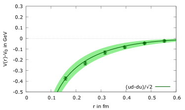
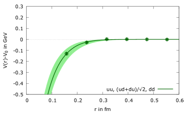
Figure 1: (left) $(I=0,j=0)$ potential. (right) $(I=1,j=1)$ potential.

The existence or non-existence of a stable tetraquark and its binding energy depends on the light quark mass $q$ [7]. Thus, we have performed computations of $\bar{Q}\bar{Q}$ potentials for three different light $u$ and $d$ quark masses corresponding to $m_{\pi}\in\{340\,\textrm{MeV},480\,\textrm{MeV},650\,\textrm{MeV}\}$. The results, which can be parameterized by a screened Coulomb potential

$$V(r)=-\frac{\alpha}{r}e^{-r^{2}/d^{2}},$$ (1)

have been extrapolated to $m_{\pi}=140\,\textrm{MeV}$ [8]. The parameterization (1) is motivated by one-gluon exchange for small $\bar{Q}\bar{Q}$ separations $r$ and the formation of two $B$ mesons at larger $r$ as a consequence of color screening as sketched in Figure 2. Even though this approach is phenomenologically motivated, it is fully consistent with our lattice QCD results, i.e. the corresponding fits yield small $\chi^{2}/\textrm{dof}$. The numerical values of the parameters $\alpha$ and $d$ are collected for both potentials in Table 1. Clearly, the $(I=0,j=0)$ potential is more attractive than the $(I=1,j=1)$ potential.

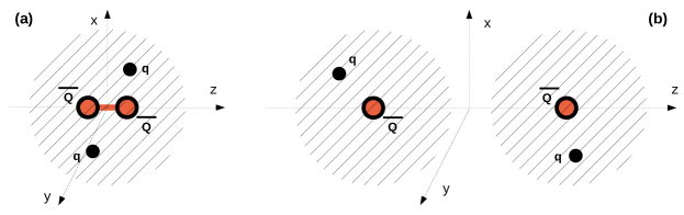
Figure 2: (a) At small separations the static antiquarks $\bar{Q}\bar{Q}$ interact by perturbative one-gluon exchange. (b) At large separations the light quarks $qq$ screen the interaction and the four quarks form two rather weakly interacting $B$ mesons.

$I$	$j$	$\alpha$	$d$ in fm
$\ 0\$	$\ 0\$	$\ 0.34^{+0.03}_{-0.03}\$	$\ 0.45^{+0.12}_{-0.10}\$
$1$	$1$	$0.29^{+0.05}_{-0.06}$	$0.16^{+0.05}_{-0.02}$

Table 1: Parameters $\alpha$ and $d$ of the parameterization (1) of the two attactive $\bar{Q}\bar{Q}$ potentials with $(I=0,j=0)$ and $(I=1,j=1)$.

The potential parameterization (1) with $\alpha$ and $d$ from Table 1 can be inserted into the Schrödinger equation, i.e. they can be used to explore the existence of stable tetraquarks or tetraquark resonances in the Born-Oppenheimer approximation. A stable $\bar{b}\bar{b}ud$ tetraquark with quantum numbers $I(J^{P})=0(1^{+})$ around $60\,\textrm{MeV}$ below the $BB^{\ast}$ threshold has been predicted in [5, 7, 8, 9]. The search for $\bar{b}\bar{b}ud$ tetraquark resonances is discussed in [13] and the following sections.

3 The emergent wave method

In this section we discuss the emergent wave method, which allows to extract phase shifts and resonance parameters. More details can be found e.g. in [12].

We start by considering the Schrödinger equation

$$\Big{(}H_{0}+V(r)\Big{)}\Psi=E\Psi$$ (2)

and by splitting the wave function into two parts,

$$\Psi=\Psi_{0}+X.$$ (3)

$\Psi_{0}$ is the incident wave, which is a solution of the free Schrödinger equation, i.e. $H_{0}\Psi_{0}=E\Psi_{0}$, and $X$ denotes the emergent wave. Inserting eq. (3) into eq. (2) and using the free Schrödinger equation we obtain

$$\Big{(}H_{0}+V(r)-E\Big{)}X=-V(r)\Psi_{0}.$$ (4)

Solving this equation for given energy $E$ provides the emergent wave $X$. The asymptotic behavior of $X$ determines the phase shifts. We find the poles of the S matrix and the T matrix in the complex energy plane and identify them with resonances, when located in the second Riemann sheet at $\mathcal{E}-i\Gamma/2$, where $\mathcal{E}$ is the energy and $\Gamma$ is the decay width of the resonance.

3.1 Partial wave decomposition

The Hamiltonian describing the two heavy antiquarks $\bar{b}\bar{b}$ is

$$H=H_{0}+V(r)=-\frac{\hbar^{2}}{2\mu}\triangle+V(r),$$ (5)

where $\mu=M/2$ is the reduced mass and $M=5\,280\,\textrm{MeV}$ is the mass of the $B$ meson from the PDG [14]. One can express the incident plane wave $\Psi_{0}=e^{i\mathbf{k}\cdot\mathbf{r}}$ as a sum over spherical waves,

$$\Psi_{0}=e^{i\mathbf{k}\cdot\mathbf{r}}=\sum_{l}(2l+1)i^{l}j_{l}(kr)P_{l}(\hat{\mathbf{k}}\cdot\hat{\mathbf{r}}),$$ (6)

where $j_{l}$ are spherical Bessel functions, $P_{l}$ are Legendre polynomials and the relation between energy and momentum is $\hbar k=\sqrt{2\mu E}$. Since the potential $V(r)$ is spherically symmetric, we can also expand the emergent wave $X$ in terms of Legendre polynomials $P_{l}$,

$$X=\sum_{l}(2l+1)i^{l}\frac{\chi_{l}(r)}{kr}P_{l}(\hat{\mathbf{k}}\cdot\hat{\mathbf{r}}).$$ (7)

Inserting eq. (6) and eq. (7) into eq. (4) leads to a set of ordinary differential equations for $\chi_{l}$,

$$\bigg{(}-\frac{\hbar^{2}}{2\mu}\frac{d^{2}}{dr^{2}}+\frac{l(l+1)}{2\mu r^{2}}+V(r)-E\bigg{)}\chi_{l}(r)=-V(r)krj_{l}(kr).$$ (8)

3.2 Solving the differential equations for the emergent wave

$V(r)$, eq. (1), is exponentially screened, i.e. $V(r)\approx 0$ for $r\geq R$, where $R\gg d$. Consequently, the emergent wave is a superposition of outgoing spherical waves for large separations $r\geq R$ and can be expressed by spherical Hankel functions of the first kind $h_{l}^{(1)}$,

$$\frac{\chi_{l}(r)}{kr}=it_{l}h_{l}^{(1)}(kr).$$ (9)

To compute the complex prefactors $t_{l}$, which will lead to the phase shifts, we solve the ordinary differential equation (8) using the following boundary conditions:

• At $r=0$: $\chi_{l}(r)\propto r^{l+1}$.

• For $r\geq R$: eq. (9).

We emphasize that the boundary condition for $r\geq R$ depends on $t_{l}$. Solving the differential equation for a given value of the energy $E$, this boundary condition is only fulfilled for a specific value of $t_{l}$. In other words the boundary condition for $r\geq R$ fixes $t_{l}$ as a function of $E$.

To solve eq. (8) numerically, we have implemented two different approaches:

• A fine uniform discretization of the interval $[0,R]$ reducing the differential equation to a large set of linear equations, which can be solved rather efficiently, since the corresponding matrix is tridiagonal.

• A standard 4-th order Runge-Kutta shooting method.

3.3 Phase shifts, S and T matrix poles

$t_{l}$ is an eigenvalue of the T matrix (see standard textbooks on quantum mechanics and scattering, e.g. [15]). From $t_{l}$ we can determine the phase shift $\delta_{l}$ and also the corresponding S matrix eigenvalue

$$s_{l}\equiv 1+2it_{l}=e^{2i\delta_{l}}$$ (10)

(at large distances $r\geq R$ the radial wave function is $kr(j_{l}(kr)+it_{l}h_{l}^{(1)}(kr))=(kr/2)(h_{l}^{(2)}(kr)+e^{2i\delta_{l}}h_{l}^{(1)}(kr))$). Note that both the S matrix and the T matrix are analytical in the complex plane and are also defined for complex energies $E$. Thus, we solve the differential equation (8) for complex $E$ and find the S and T matrix poles by scanning the complex energy plane $(\textrm{Re}(E),\textrm{Im}(E))$ and by applying Newton’s method to find the roots of $1/t_{l}(E)$. These poles correspond to complex resonance energies $E=\mathcal{E}-i\Gamma/2$ and must be located in the second Riemann sheet with a negative imaginary part of $E$.

4 Results for phase shifts, S and T matrix poles and prediction of resonances

4.1 Phase shifts $\delta_{l}$

We consider the more attractive $\bar{b}\bar{b}$ potential with $(I=0,j=0)$ (cf. section 2), compute $t_{l}$ for real energies $E$ and apply eq. (10) to determine phase shifts $\delta_{l}$ for orbital angular momenta $l=0,1,2,3,4$. A clear indication for a resonance would be a strongly increasing $\delta_{\textit{{l}}}$ from $0$ to almost $\pi$. Such a behavior is, however, not observed (cf. Figure 3 (left)). Thus, we have to check more thoroughly, whether there are resonances or not.

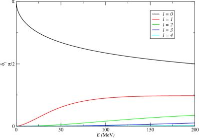
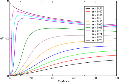
Figure 3: (left) Phase shift $\delta_{l}$ as a function of the energy $E$ for orbital angular momenta $l=0,1,2,3,4$ for the $(I=0,j=0)$ potential ($\alpha=0.34$, $d=0.45\,\textrm{fm}$). (right) Phase shift $\delta_{1}$ as a function of the energy $E$ for different $\alpha$ and fixed $d=0.45\,\textrm{fm}$.

It is also interesting to consider the $l=1$ channel for even more attractive potentials by increasing the parameter $\alpha$, while $d$ is fixed. We show the resulting phase shifts $\delta_{1}$ in Figure 3 (right). For $\alpha\gtrsim 0.65$ resonances are clearly indicated. For $\alpha\gtrsim 0.72$ there are even bounds states, i.e. the phase shifts start at $\pi$ and decrease monotonically. However, this observation does not allow to make a clear statement, whether there is a resonance for $\alpha=0.34$.

4.2 Resonances as poles of the S and T matrices for complex energies $E$

Now we search for poles of the T matrix eigenvalue $t_{l}$ in the complex energy plane, which indicate resonances. For orbital angular momentum $l=1$ and the $(I=0,j=0)$ potential we find a pole, which is shown in Figure 4 (left), where $t_{1}$ is plotted as a function of the complex energy $E$. For a better understanding of the resonance and its dependence on the potential we determine the pole of $t_{1}$ for various parameters $\alpha$. In Figure 4 (right) we show the location of the pole for several values of $\alpha$ in the $(\textrm{Re}(E),\textrm{Im}(E))$ plane. Indeed, starting at $\alpha=0.21$ we find poles. Consequently, we can predict a resonance at $\alpha=0.34$. For orbital angular momenta $l>1$ as well as for the less attractive potential $(I=1,j=1)$ no poles have been found.

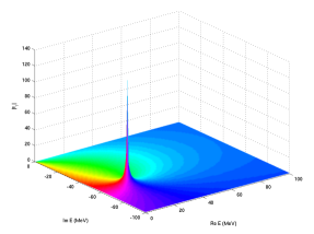
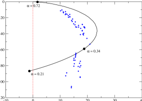
Figure 4: (left): T matrix eigenvalue $t_{1}$ as a function of the complex energy $E$ for the $(I=0,j=0)$ potential ($\alpha=0.34$, $d=0.45\,\textrm{fm}$). Along the vertical axis we show the norm $|t_{1}|$, while the phase $\textrm{arg}(t_{1})$ is visualized by different colors. (right) Trajectory of the pole of the T matrix eigenvalue $t_{1}$ in the complex energy plane $(\textrm{Re}(E),\textrm{Im}(E))$ corresponding to a variation of the parameter $\alpha$. The cloud of blue points represents the systematic error of our prediction.

4.3 Analysis of statistical and systematic errors

We perform a detailed statistical and systematic error analysis for the pole of $t_{1}$ in the complex energy plane $(\textrm{Re}(E),\textrm{Im}(E))$ using the same method as for our study of bound states [7]. We parametrize the lattice QCD data for the potential $V^{\textrm{lat}}(r)$ with an uncorrelated $\chi^{2}$ minimizing fit using the ansatz (1), i.e. we minimize the expression

$$\chi^{2}=\sum_{r_{\textrm{min}}\leq r\leq r_{\textrm{max}}}\bigg{(}\frac{V(r)-V^{\textrm{lat}}(r)}{\Delta V^{\textrm{lat}}(r)}\bigg{)}^{2}$$ (11)

with respect to $\alpha$ and $d$, where $\Delta V^{\textrm{lat}}(r)$ denotes the corresponding statistical errors. To estimate the systematic error, we perform fits for various fit ranges $r_{\textrm{min}}\leq r\leq r_{\textrm{max}}$. Additionally, we vary the range of the temporal separation $t_{\textrm{min}}\leq t\leq t_{\textrm{max}}$, where $V^{\textrm{lat}}(r)$ is read off. For each fit we determine the pole of $t_{1}$, i.e. the resonance energy $\mathcal{E}$ and the decay width $\Gamma$. As systematic error we take the spread of these results, while the statistical error is determined via the jackknife method. Applying this combined systematic and statistical error analysis, we find a resonance energy $\mathcal{E}=\textrm{Re}(E)=17^{+4}_{-4}\,\textrm{MeV}$ above the $BB$ threshold and a decay width $\Gamma=-2\textrm{Im}(E)=112^{+90}_{-103}\,\textrm{MeV}$. Studying the symmetries of the quarks with respect to color, flavor, spin and their spatial wave function and considering the Pauli principle we determine the quantum numbers as $I(J^{P})=0(1^{-})$. The mass of this $\bar{b}\bar{b}ud$ tetraquark resonance is given by $m=2M+\textrm{Re}(E)=10\,576^{+4}_{-4}\,\textrm{MeV}$.

5 Conclusion

We have explored the existence of $\bar{b}\bar{b}ud$ tetraquark resonances applying lattice QCD potentials for two static antiquarks in the presence of two light quarks, the Born-Oppenheimer approximation and the emergent wave method. We predict a new resonance with quantum numbers $I(J^{P})=0(1^{-})$, a resonance mass $\textrm{Re}(E)=17^{+4}_{-4}\,\textrm{MeV}$ and a decay width $\Gamma=112^{+90}_{-103}\,\textrm{MeV}$.

References

- [1] W. Detmold, K. Orginos and M. J. Savage, “ Potentials in Quenched Lattice QCD,” Phys. Rev. D 76, 114503 (2007) [hep-lat/0703009 [hep-lat]].
- [2] M. Wagner [ETM Collaboration], “Forces between static-light mesons,” PoS LATTICE 2010, 162 (2010) [arXiv:1008.1538 [hep-lat]].
- [3] G. Bali et al. [QCDSF Collaboration], “Static-light meson-meson potentials,” PoS LATTICE 2010, 142 (2010) [arXiv:1011.0571 [hep-lat]].
- [4] M. Wagner [ETM Collaboration], “Static-static-light-light tetraquarks in lattice QCD,” Acta Phys. Polon. Supp. 4, 747 (2011) [arXiv:1103.5147 [hep-lat]].
- [5] P. Bicudo et al. [European Twisted Mass Collaboration], “Lattice QCD signal for a bottom-bottom tetraquark,” Phys. Rev. D 87, 114511 (2013) [arXiv:1209.6274 [hep-ph]].
- [6] Z. S. Brown and K. Orginos, “Tetraquark bound states in the heavy-light heavy-light system,” Phys. Rev. D 86, 114506 (2012) [arXiv:1210.1953 [hep-lat]].
- [7] P. Bicudo, K. Cichy, A. Peters, B. Wagenbach and M. Wagner, “Evidence for the existence of and the non-existence of and tetraquarks from lattice QCD,” Phys. Rev. D 92, 014507 (2015) [arXiv:1505.00613 [hep-lat]].
- [8] P. Bicudo, K. Cichy, A. Peters and M. Wagner, “ interactions with static bottom quarks from Lattice QCD,” Phys. Rev. D 93, 034501 (2016) [arXiv:1510.03441 [hep-lat]].
- [9] P. Bicudo, J. Scheunert and M. Wagner, “Including heavy spin effects in the prediction of a tetraquark with lattice QCD potentials,” Phys. Rev. D 95, 034502 (2017) [arXiv:1612.02758 [hep-lat]].
- [10] A. Francis, R. J. Hudspith, R. Lewis and K. Maltman, “Lattice prediction for deeply bound doubly heavy tetraquarks,” Phys. Rev. Lett. 118, 142001 (2017) [arXiv:1607.05214 [hep-lat]].
- [11] P. Junnarkar, N. Mathur and M. Padmanath, “Study of doubly heavy tetraquarks in Lattice QCD,” arXiv:1810.12285 [hep-lat].
- [12] P. Bicudo and M. Cardoso, “Tetraquark bound states and resonances in the unitary and microscopic triple string flip-flop quark model, the light-light-antiheavy-antiheavy case study,” Phys. Rev. D 94, 094032 (2016) [arXiv:1509.04943 [hep-ph]].
- [13] P. Bicudo, M. Cardoso, A. Peters, M. Pflaumer and M. Wagner, “ tetraquark resonances with lattice QCD potentials and the Born-Oppenheimer approximation,” Phys. Rev. D 96, 054510 (2017) [arXiv:1704.02383 [hep-lat]].
- [14] M. Tanabashi et al. [Particle Data Group], “Review of particle physics,” Phys. Rev. D 98, 030001 (2018).
- [15] E. Merzbacher, “Quantum mechanics (3rd edition),” Wiley (1998).