Competing chemical and hydrodynamic interactions in autophoretic colloidal suspensions

Abstract

At the surfaces of autophoretic colloids, slip velocities arise from local chemical gradients that are many-body functions of particle configuration and activity. For rapid chemical diffusion, coupled with slip-induced hydrodynamic interactions, we deduce the chemohydrodynamic forces and torques between colloids. For bottom-heavy particles above a no-slip wall, the forces can be expressed as gradients of a non-equilibrium potential which, by tuning the type of activity, can be varied from repulsive to attractive. When this potential has a barrier, we find arrested phase separation with a mean cluster size set by competing chemical and hydrodynamic interactions. These are controlled, in turn, by the monopolar and dipolar contributions to the active chemical surface fluxes.

I Introduction

Non-equilibrium processes, of biological Brennen and Winet (1977) or chemical Anderson (1989); Ebbens and Howse (2010) origin, when confined to a thin layer around a colloidal particle, create interfacial slip flows. These drive exterior fluid flows, which mediate long-ranged hydrodynamic interactions between particles Singh et al. (2015); Singh and Adhikari (2016, 2018); Thutupalli et al. (2018). In instances where the slip is of biological origin, as for example in suspensions of Volvox Goldstein (2015); Pedley (2016), the slip on any one particle is typically independent of the configuration and slip of other particles. Motion under the active hydrodynamic forces and torques thereby computed Singh et al. (2015); Singh and Adhikari (2016, 2018) is in excellent agreement with experiment Petroff et al. (2015); Thutupalli et al. (2018). However, when slip is induced by gradients of chemical species, as for example in autophoretic colloids Palacci et al. (2013); Ebbens and Howse (2010), the gradient at the location of one particle is determined by the chemical fields of all other particles, causing the slip to be a many-body function of the colloidal configurations and activities. Interactions in autophoretic suspensions thus have both chemical and hydrodynamic many-body contributions. A quantitative theory of these is necessary to understand the dynamics and non-equilibrium steady-states of such suspensions.

Experiments on active suspensions are often performed in the vicinity of a plane boundary, for example a no-slip wall Theurkauff et al. (2012); Buttinoni et al. (2013); Palacci et al. (2013). Here, aggregation of colloids to a self-limiting cluster size that is proportional to the self-propulsion speed has been reported. This cannot be explained by current theories Pohl and Stark (2014); Saha et al. (2014); Liebchen et al. (2017); Yan and Brady (2016), which typically only account for chemical (not hydrodynamic) many-body effects. (Many-body chemohydrodynamics have recently been addressed, but not near a wall Liebchen and Löwen (2018); Popescu et al. (2018).) While it has been shown that translational and rotational diffusiophoretic motion in overlapping chemical fields can induce aggregation Pohl and Stark (2014), this predicts instead a decrease in the size of aggregates with self-propulsion speed Theurkauff et al. (2012); Buttinoni et al. (2013). In other work, aggregation has been attributed to the tendency of particles to propel away from the chemical they produce Liebchen et al. (2015, 2017) leading to formation of patterns. So far, all of the above theories ignore the local conservation of momentum and/or the role played by plane boundaries as barriers to chemical flux and sinks of fluid momentum. A theory which consistently accounts for these effects remains lacking.

Here we present a microscopic theory for autophoretic colloids in the proximity of boundaries, restricting attention, for simplicity, to cases governed by a single chemical diffusant species. We construct the slip on one particle as a many-body function of the position and activity of all others. The slip is obtained from the solution of the diffusion equation, in the limit of zero Péclet number, and then used in the momentum equation, in the limit of zero Reynolds number, to compute chemohydrodynamic forces and torques between the colloids.

These forces and torques generically do not admit potentials and explicitly violate the action-reaction principle Soto and Golestanian (2014). However, for bottom-heavy particles located above and oriented normal to a plane boundary where the chemical flux and fluid flow vanish, the bulk flow is predominantly irrotational and, strikingly, the interactions can after all be written as gradients of a non-equilibrium pair potential. To leading order, this potential depends on the ratio, $\alpha$, of the magnitudes of monopolar and dipolar chemical activity of the colloids (see below) and can be varied, by tuning this ratio, from purely repulsive to purely attractive. This leads to colloidal steady-states that are, respectively, liquid-like and crystalline. When instead the potential has a barrier, phase separation can arrest to a self-limiting cluster size that is set by $\alpha$.

In what follows, we explain how these results are derived, starting in Section II with our solution of the chemohydrodynamic traction in the presence of fast diffusant. Section III applies our formalism to the case of bottom-heavy particles near an infinite plane horizontal no-flux, no-slip wall and we conclude with a brief discussion in Section IV.

II Many-body Chemohydrodynamics

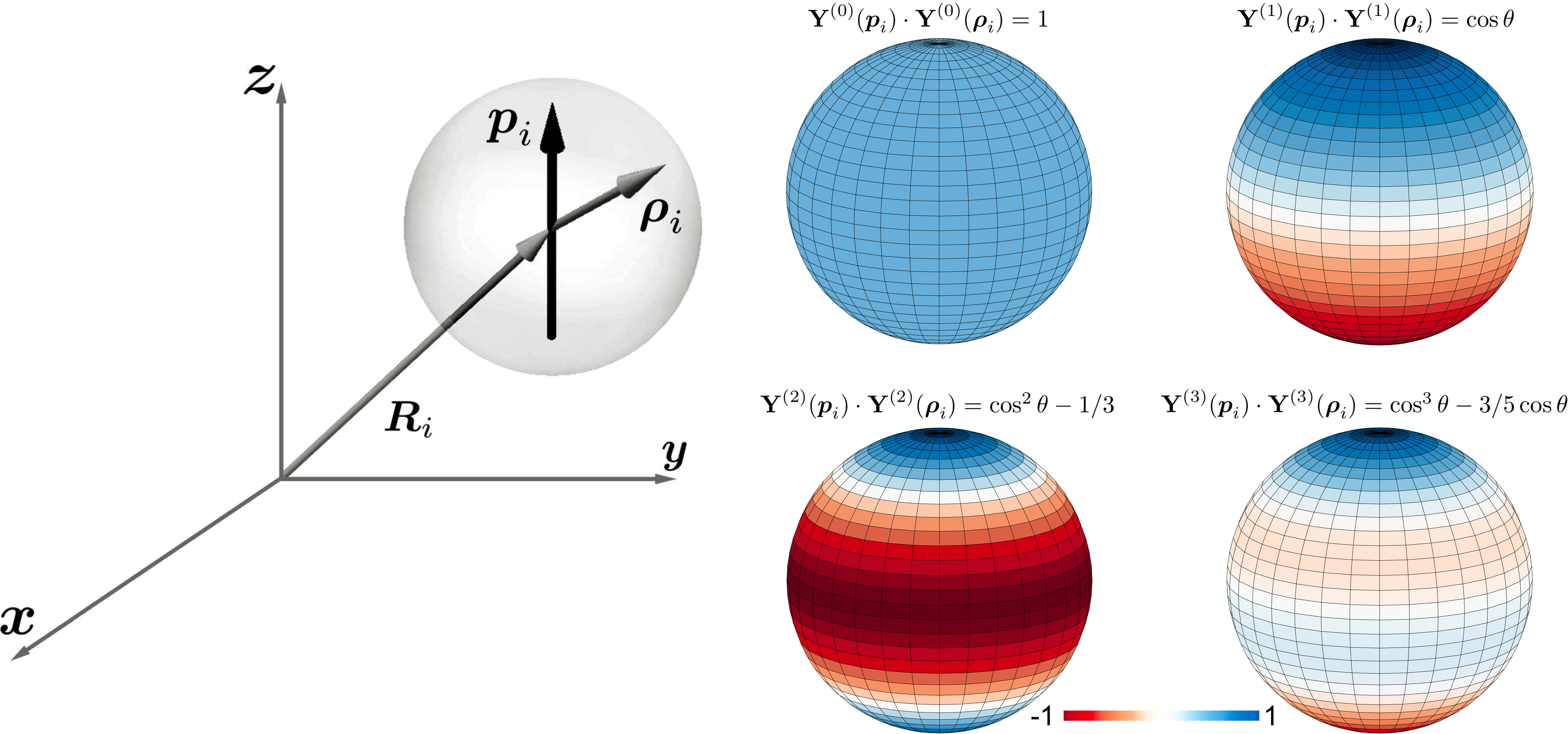
Figure 1: The left panel shows the system of coordinates used to describe the kinematics of active colloids. The $i$-th colloid is centered at $\boldsymbol{R}_{i}$, oriented along the unit vector $\boldsymbol{p}_{i}$, and has radius vector $\boldsymbol{\rho}_{i}$. The right panel shows the tensorial modes, $\mathbf{Y}_{i}^{(m)}(\bm{p}_{i})\cdot\mathbf{Y}^{(m)}(\bm{\hat{\rho}}_{i})$, of an uniaxial surface scalar field with the direction of axial symmetry along the $z$-axis, for $m=0,\ldots 3$.

We consider a suspension of $N$ chemically active spherical colloids of radius $b$ in an incompressible fluid of viscosity $\eta$. The $i$-th sphere is centered at $\boldsymbol{R}_{i}$, has radius vector $\boldsymbol{\rho}_{i}$, and is oriented along $\boldsymbol{p}_{i}$ with the points $\boldsymbol{r}_{i}=\boldsymbol{R}_{i}+\boldsymbol{\rho}_{i}$ defining its surface $S_{i}$. The system of coordinates is shown in Fig.(1). Here we restrict ourselves to the limit of rapid Fickian diffusion of chemical and rapid viscous transport of momentum. Then, the chemical field $c$ obeys the steady-state diffusion equation $\boldsymbol{\nabla}\cdot\boldsymbol{j}=0$ in the bulk where $\boldsymbol{j}=-D\boldsymbol{\nabla}c$ is the diffusive flux with diffusivity $D$. The chemical reaction determines the normal component of the flux at the boundaries,

$$\boldsymbol{j}(\boldsymbol{r})\cdot\hat{\boldsymbol{\rho}_{i}}=j^{\mathcal{A}}(\boldsymbol{\rho}_{i})\qquad(\boldsymbol{r}\in S_{i}).$$ (1)

Here and below, fields that are restricted to the surfaces $S_{i}$ carry arguments $\boldsymbol{\rho}_{i}$. The slip flow produced by chemical gradients is

$$\boldsymbol{v}^{\mathcal{A}}(\boldsymbol{\rho}_{i}) =\mu_{c}(\boldsymbol{\rho}_{i})\boldsymbol{\nabla}_{s}\,c(\boldsymbol{\rho}_{i}),$$ (2)

where $\boldsymbol{\nabla}_{s}$ is the surface gradient and $\mu_{c}(\boldsymbol{\rho}_{i})$ is the phoretic mobility Anderson (1989). The flow field $\boldsymbol{v}$ obeys the momentum balance equation $\boldsymbol{\nabla}\cdot\boldsymbol{\sigma}=0$ where $\boldsymbol{\sigma}=-p\boldsymbol{I}+\eta(\bm{\nabla}\boldsymbol{v}+(\bm{\nabla}\boldsymbol{v})^{T})$ is the Cauchy stress in an incompressible Newtonian fluid and $\boldsymbol{I}$ is the identity tensor. The slip flow modifies the usual no-slip boundary condition on a colloid translating with velocity $\mathbf{V}_{i}$ and rotating with angular velocity $\mathbf{\Omega}_{i}$ to

$$\boldsymbol{v}(\boldsymbol{r}) =\mathbf{V}_{i}+\mathbf{\Omega}_{i}\times\boldsymbol{\rho}_{i}+\boldsymbol{v}^{\mathcal{A}}(\boldsymbol{\rho}_{i})\qquad(\boldsymbol{r}\in S_{i}).$$ (3)

The chemohydrodynamic problem is to determine the Cauchy stress in the bulk and the traction at the boundaries in terms of the prescribed active flux $j^{\mathcal{A}}$. The linearity of the diffusion and Stokes equations and their respective boundary conditions, together with the linearity of slip flow equation that couples them, makes it possible to obtain a formally exact solution to the chemohydrodynamic problem. We show this below.

First, we take advantage of the spherical symmetry of the colloids to parametrize the fields on their surfaces in terms of the $l$-th rank irreducible tensorial harmonics $\mathbf{Y}^{(l)}(\bm{\hat{\rho}})=(-1)^{l}\rho^{l+1}\boldsymbol{\nabla}^{l}\rho^{-1}$. The expansion of the surface concentration and surface flux are

$$c(\boldsymbol{\rho}_{i}) =\sum_{m=0}^{\infty}w_{m}\mathbf{C}_{i}^{(m)}\cdot\mathbf{Y}^{(m)}(\bm{\hat{\rho}}_{i}),$$ (4a)

$$j^{\mathcal{A}}(\boldsymbol{\rho}_{i}) =\sum_{m=0}^{\infty}\tilde{w}_{m}\mathbf{J}_{i}^{(m)}\cdot\mathbf{Y}^{(m)}(\bm{\hat{\rho}}_{i}),\quad(\text{specified})$$ (4b)

where $\mathbf{C}_{i}^{(l)}$ and $\mathbf{J}_{i}^{(l)}$ are $l$-th rank symmetric irreducible tensorial coefficients with $(2l+1)$ independent components Hess (2015). Here and below, a maximal contraction of two tensors is denoted by a dot product. The coefficients $\mathbf{J}_{i}^{(m)}$ are specified as part of the problem and, for uniaxially symmetric activity, can be be parametrized as $\mathbf{J}_{i}^{(m)}=J^{(m)}\mathbf{Y}^{(m)}(\bm{p}_{i})$, reducing the number of free parameters considerably. The first four uniaxial tensorial surface modes are shown in Fig.(1). The corresponding expansions for the active slip and the traction are

$$\boldsymbol{v}^{\mathcal{A}}(\boldsymbol{\rho}_{i}) =\sum_{l=1}^{\infty}w_{l-1}\mathbf{V}_{i}^{(l)}\cdot\mathbf{Y}^{(l-1)}(\bm{\hat{\rho}}_{i}),\quad$$ (5a)

$$\boldsymbol{f}^{\mathcal{A}}(\boldsymbol{\rho}_{i}) =\sum_{l=1}^{\infty}\tilde{w}_{l-1}\mathbf{F}_{i}^{(l)}\cdot\mathbf{Y}^{(l-1)}(\bm{\hat{\rho}}_{i}),\quad(\text{sought})$$ (5b)

where $\mathbf{V}_{i}^{(l)}$ and $\mathbf{F}_{i}^{(l)}$ are $l$-th rank tensorial coefficients, symmetric and irreducible in their last $l-1$ indices, with the dimensions of force and velocity respectively. The $l$-dependent expansion weights are

$$w_{l}=\frac{1}{l!(2l-1)!!},\qquad\tilde{w}_{l}=\frac{2l+1}{4\pi b^{2}},$$ (6)

and unless otherwise specified, sums over repeated indices $m,m^{\prime}$ start from $0$ while sums over repeated indices $l,l^{\prime}$ start from $1$.

Second, linearity of the diffusion equation and the boundary conditions implies that the tensorial coefficients of the surface concentration and surface flux are linearly related,

$$\mathbf{C}_{i}^{(m)}=-\boldsymbol{\varepsilon}{}_{ik}^{(m,m^{\prime})}\cdot\mathbf{J}_{k}^{(m^{\prime})}.$$ (7)

In the above, repeated harmonic ($m,m^{\prime}$) and particle ($i,k$) indices are summed over. The coefficients of proportionality, $\boldsymbol{\varepsilon}{}_{ik}^{(m,m^{\prime})}$, are tensors of rank $(m+m^{\prime})$ and many-body functions of the particle positions. Maxwell, in his study of the capacitance of a system of spherical conductors, called the coefficients $\boldsymbol{\varepsilon}{}_{ik}^{(0,0)}$ elastances Maxwell (1873). We call the complete set of coefficients generalized elastance tensors.

Third, linearity of the slip equation implies that the tensorial coefficients of the slip and surface concentration are linearly related,

$$\mathbf{V}_{i}^{(l)}=- \boldsymbol{\chi}^{(l,m)}\cdot\mathbf{C}_{i}^{(m)},$$ (8)

where $\boldsymbol{\chi}^{(l,m)}$ is a coupling tensor of rank $(l+m)$ that depends on the phoretic mobility $\mu_{c}.$ We assume the latter to not vary between particles, making the coupling tensors independent of the particle indices.

Fourth, linearity of the Stokes equation and the boundary conditions implies that the tensorial coefficients of the slip and traction are linearly related,

$$\mathbf{F}_{i}^{(l)} = -\boldsymbol{\gamma}_{ik}^{(l,l^{\prime})}\cdot\mathbf{V}_{k}^{(l^{\prime})},$$ (9)

where the coefficients of proportionality, $\boldsymbol{\gamma}_{ik}^{(l,l^{\prime})}$, are tensors of rank $(l+l^{\prime})$ and many-body functions of the particle positions. We call the complete set of coefficients the generalized friction tensors Singh and Adhikari (2018).

Finally, eliminating the coefficients of the concentration and slip between the preceding three equations, we obtain a direct relation between the prescribed coefficients of the active flux and the sought coefficients of the traction,

$$\mathbf{F}_{i}^{(l)}=-\underbracket{\boldsymbol{\gamma}_{ij}^{(l,l^{\prime})}}_{\text{Stokes}}\cdot\boldsymbol{\chi}^{(l^{\prime},m^{\prime})}\cdot\underbracket{\boldsymbol{\varepsilon}{}_{jk}^{(m^{\prime},m)}}_{\text{Laplace}}\cdot\mathbf{J}{}_{k}^{(m)}.$$ (10)

This shows that the force per unit area on autophoretic colloids has both many-body chemical and hydrodynamic contributions encoded, respectively, in the generalized elastance and friction tensors and determined, respectively, by solutions of the Laplace and Stokes equations. Ignoring chemical (hydrodynamic) interactions between particles amounts to setting the components of the elastance (friction) tensors off-diagonal in the particle indices to zero. The coefficients $\mathbf{F}_{i}^{(1)}$ and $b\boldsymbol{\,\epsilon}\cdot\mathbf{F}_{i}^{(2)}$, where $\boldsymbol{\epsilon}$ is the Levi-Civita tensor, are the active force and torque on the $i$-th colloid that determine its rigid body motion. The remaining coefficients are required to determine suspension-scale quantities such as the rheological response and the power dissipation Singh and Adhikari (2018). The formal solution above is completed by providing expressions for the elastance, coupling and friction tensors.

The coupling tensors are obtained straightforwardly from the slip flow equation Eq.(8) with a prescribed mobility,

$$\boldsymbol{\chi}^{(l,m)}=-\int\tilde{w}_{l-1}\mathbf{Y}^{(l-1)}(\hat{\bm{\rho}}_{i})\mu_{c}(\boldsymbol{\rho}_{i})w_{m}\boldsymbol{\nabla}_{s}\mathbf{Y}^{(m)}(\hat{\bm{\rho}}_{i})\,dS_{i}.$$ (11)

The elastance tensors are most conveniently obtained from the solution of the boundary integral representation of the Laplace equation. To leading order in distance, they assume a pairwise form given in terms of gradients of the Green’s function $H$ of the Laplace equation,

$$-\boldsymbol{\varepsilon}_{ik}^{(m,m^{\prime})}\approx b^{m+m^{\prime}}\bm{\nabla}_{{\scriptscriptstyle\boldsymbol{R}_{i}}}^{m}\bm{\nabla}_{{\scriptscriptstyle\boldsymbol{R}_{k}}}^{m^{\prime}}H(\boldsymbol{R}_{i},\boldsymbol{R}_{k}).$$

A method for calculating their many-body forms, to any desired order of accuracy, is provided in the Appendix A. The generalized friction tensors are similarly obtained from the boundary integral representation of the Stokes equation Singh and Adhikari (2018). To leading order in distance, they assume a pairwise form given in terms of gradients of the Green’s function $\mathbf{G}$ of the Stokes equation

$$-\boldsymbol{\gamma}_{ik}^{(l,\,l^{\prime})}\approx b^{l+l^{\prime}-2}\bm{\nabla}_{{\scriptscriptstyle\boldsymbol{R}_{i}}}^{l-1}\bm{\nabla}_{{\scriptscriptstyle\boldsymbol{R}_{k}}}^{l^{\prime}-1}\mathbf{G}(\boldsymbol{R}_{i},\boldsymbol{R}_{k}).$$

A method for calculating them, to any desired order of accuracy, has been presented earlier Singh and Adhikari (2018). Combining the three preceding equations with Eq.(10) gives explicit expressions for the active traction in terms of the particle positions, orientations and activities. The Cauchy stress in the fluid is then determined by the integral representation that relates it to the traction Ghose and Adhikari (2014); Singh and Adhikari (2018).

We now derive the dynamical equations for autophoretic motion of the colloids from the balance of forces and torques. The active force $\mathbf{F}_{i}^{\mathcal{A}}$ and torque $\mathbf{T}_{i}^{\mathcal{A}}$ on the $i$-th colloid follows from the first two modes of the active traction in (10):

$$\mathbf{F}_{i}^{\mathcal{A}} =-\boldsymbol{\gamma}_{ij}^{(T,l)}\cdot\boldsymbol{\chi}^{(l,m^{\prime})}\cdot\boldsymbol{\varepsilon}{}_{jk}^{(m^{\prime},m)}\cdot\mathbf{J}{}_{k}^{(m)},$$ (12a)

$$\mathbf{T}_{i}^{\mathcal{A}} =-\boldsymbol{\gamma}_{ij}^{(R,l)}\cdot\boldsymbol{\chi}^{(l,m^{\prime})}\cdot\boldsymbol{\varepsilon}{}_{jk}^{(m^{\prime},m)}\cdot\mathbf{J}{}_{k}^{(m)}.$$ (12b)

where $\boldsymbol{\gamma}_{ij}^{(T,l)}=\boldsymbol{\gamma}_{ij}^{(1,l)}$ and $\boldsymbol{\gamma}_{ij}^{(R,l)}=\boldsymbol{\epsilon}\cdot\boldsymbol{\gamma}_{ij}^{(2,l)}$. The drag forces and torques are given by the standard expressions Mazur and Saarloos (1982); Ladd (1988)

$$\mathbf{F}_{i}^{\mathcal{D}} =-\boldsymbol{\gamma}_{ik}^{TT}\cdot\mathbf{V}_{k}-\boldsymbol{\gamma}_{ik}^{TR}\cdot\boldsymbol{\Omega}_{k},$$ (13a)

$$\mathbf{T}_{i}^{\mathcal{D}} =-\boldsymbol{\gamma}_{ik}^{RT}\cdot\mathbf{V}_{k}-\boldsymbol{\gamma}_{ik}^{RR}\cdot\boldsymbol{\Omega}_{k}.$$ (13b)

Conservative body forces and torques, $\mathbf{F}_{i}^{\mathcal{P}}$ and $\mathbf{T}_{i}^{\mathcal{P}}$, may, in addition, act on the particles. Then, Newton’s equations for the $i$-th colloid are

$$M\dot{\mathbf{V}}_{i}=\mathbf{F}_{i}^{\mathcal{A}}+\mathbf{F}_{i}^{\mathcal{D}} +\mathbf{F}_{i}^{\mathcal{P}},$$ (14a)

$$I\dot{\mathbf{\Omega}}_{i}=\mathbf{T}_{i}^{\mathcal{A}}+\mathbf{T}_{i}^{\mathcal{D}} +\mathbf{T}_{i}^{\mathcal{P}}.$$ (14b)

where $M$ is the mass and $I$ the moment of inertia. At the colloidal scale, inertia can be ignored and Newton equations reduced to implicit algebraic equations for the velocities and angular velocities. Explicit solutions can be obtained in terms of the active forces and torques (see Appendix B) and used to evolve the position and orientation according to the kinematic equations

$$\dot{\boldsymbol{R}}_{i}=\mathbf{V}_{i},\qquad\dot{\boldsymbol{p}}_{i}=\mathbf{\Omega}_{i}\times\boldsymbol{p}_{i}.$$ (15)

Autophoretic colloidal motion is thus fully determined by the solution of the chemohydrodynamic problem.

III Autophoresis of bottom-heavy colloids near a plane wall

We now apply the above general solution to a specific, experimentally relevant, situation: autophoretic motion of particles near a planar no-flux, no-slip wall. Motivated by a minimal representation of autophoretic Janus colloids, we assume that the active surface flux $j^{\mathcal{A}}$ has monopolar and dipolar modes and that the phoretic mobility is constant,

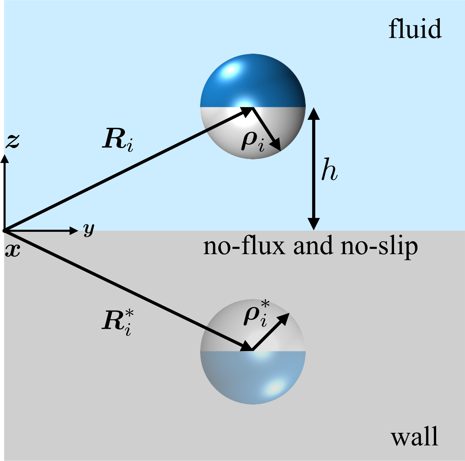
Figure 2: The system of coordinates used to describe active colloids above a planar wall. The height, $h$, of the colloid from the wall is explicitly indicated, and the system of coordinates of its image centered at $\boldsymbol{R}_{i}^{*}$ below the wall is also shown (see text). Note that in our method the fluid extends to infinity in the horizontal and upwards directions; we have no need for periodic or other boundary conditions at the edges of the simulation box. Indeed, there is no simulation box, just a set of particle coordinates which can in principle be anywhere in the upper half space.

$$4\pi b^{2}\,j^{\mathcal{A}}(\boldsymbol{\rho}_{i})=J^{(0)}+3\,J^{(1)}\boldsymbol{p}_{i}\cdot\boldsymbol{\hat{\rho}}_{i},\qquad 4\pi b^{2}\,\mu_{c}(\boldsymbol{\rho}_{i})=M^{(0)}.$$ (16)

This model has three independent parameters. The assumption of constant mobility leads to a coupling tensor with exactly one non-zero component,

$$\boldsymbol{\chi}^{(l,m)}=-\delta_{l1}\delta_{m1}\frac{M^{(0)}}{4\pi b^{3}}\boldsymbol{I},$$ (17)

corresponding to $l=m=1$. This restricts the sums in Eq.(12) for the active forces and torques to terms where the second harmonic index of the friction tensor and the first harmonic index of the elastance tensor are both equal to one. With this simplification, the active force on a colloid located at $\boldsymbol{R}_{1}$ and oriented along $\boldsymbol{p}_{1}$ contains exactly two terms:

$$\mathbf{F}_{1}^{\mathcal{\text{\text{self}}}}=-\underbrace{J^{(0)}\boldsymbol{\gamma}_{11}^{(T,1)}\cdot\boldsymbol{\varepsilon}{}_{11}^{(1,0)}}_{\text{wall-induced propulsion}} -\underbrace{J^{(1)}\boldsymbol{\gamma}_{11}^{(T,1)}\cdot\boldsymbol{\varepsilon}{}_{11}^{(1,1)}\cdot\boldsymbol{p}_{1}}_{\text{polar self-propulsion}},$$ (18)

The first term is the force arising from the broken spherical symmetry of the chemical monopole field in the vicinity of the wall and the second term is the self-propulsion force of the chemical dipole. Thus, an apolar active colloid ($J^{(0)}\neq 0,J^{(1)}=0)$ which, by symmetry, can have no motion in an unbounded medium, will acquire motion near a wall due the breaking of spherical symmetry. The scaling of the force by $-M^{(0)}/4\pi b^{3}$ in the above equation and the three equations below are for ease of display. With the introduction of a second colloid, located at $\boldsymbol{R}_{2}$ with orientation $\boldsymbol{p}_{2}$, the active force on particle $1$ will contain six additional interaction terms involving particle $2$,

$$\mathbf{F}_{1}^{\text{CI}}= -J^{(0)}\boldsymbol{\gamma}_{11}^{(T,1)}\cdot\boldsymbol{\varepsilon}{}_{12}^{(1,0)}-J^{(1)}\boldsymbol{\gamma}_{11}^{(T,1)}\cdot\boldsymbol{\varepsilon}{}_{12}^{(1,1)}\cdot\boldsymbol{p}_{2},$$ (19a)

$$\mathbf{F}_{1}^{\text{HI}}= -J^{(0)}\boldsymbol{\gamma}_{12}^{(T,1)}\cdot\boldsymbol{\varepsilon}{}_{22}^{(1,0)}-J^{(1)}\boldsymbol{\gamma}_{12}^{(T,1)}\cdot\boldsymbol{\varepsilon}{}_{22}^{(1,1)}\cdot\boldsymbol{p}_{2},$$ (19b)

$$\mathbf{F}_{1}^{\text{CHI}}= -\negmedspace\negmedspace\underbrace{J^{(0)}\boldsymbol{\gamma}_{12}^{(T,1)}\cdot\boldsymbol{\varepsilon}{}_{21}^{(1,0)}}_{\text{orientation-independent}}\negmedspace-\underbrace{J^{(1)}\boldsymbol{\gamma}_{12}^{(T,1)}\cdot\boldsymbol{\varepsilon}{}_{21}^{(1,1)}\cdot\boldsymbol{p}_{1}}_{\text{orientation-dependent}},$$ (19c)

giving a total of eight terms. Every such term is the product of an elastance tensor and a friction tensor, each of which can be diagonal or off-diagonal in the particle indices, giving four distinct kinds of interactions. Terms in which both the elastance and friction are diagonal represent self-propulsion and self-interaction forces; terms in which the elastance is off-diagonal and the friction diagonal represent chemical interactions (CI); terms in which the elastance is diagonal and the friction off-diagonal represent hydrodynamic interactions (HI); and terms in which both elastance and friction are off-diagonal represent chemohydrodynamic interactions (CHI). The CI are due to chemical gradients induced on particle $1$ due to activity of particle $2$, the HI are due to the flow incident on particle $1$ due to the slip on particle $2$ and the CHI are due to the flow incident on particle $1$ from the additional slip on particle $2$ from the chemical gradient induced on it by the activity of particle $1$. The monopolar and dipolar modes of activity yield forces that are, respectively, orientation-independent and orientation-dependent. The force on particle $2$ is obtained by interchanging indices. Structurally similar expressions are obtained for the active torques.

Explicit expressions for these forces and torques are obtained from the solutions of the linear systems defining the elastance and friction tensors, as explained in A. The coefficients of these linear systems are determined by the Green’s functions of the Laplace and Stokes equations, corresponding to the boundary conditions imposed, respectively, on the chemical and flow fields at the boundaries. Here we use solutions obtained at the second step of a Jacobi iteration, which corresponds to evaluating elastance and friction tensors to next-to-leading order in distance. We emphasize that this iteration can be continued to as many steps as needed for a prescribed accuracy. The linear system may also be solved by direct methods but we do not pursue this here. The no-flux Green’s function of the Laplace equation is

$$H^{\text{w}}(\boldsymbol{R}_{i},\boldsymbol{R}_{k})=H^{0}(\boldsymbol{r})+H^{0}(\boldsymbol{r}^{*}).$$ (20)

Here $8\pi DH^{0}(\boldsymbol{r})=\nabla^{2}r$ is the Green’s function in an unbounded domain, $\boldsymbol{r}=\boldsymbol{R}_{i}-\boldsymbol{R}_{k}$, $\boldsymbol{r}^{*}=\boldsymbol{R}_{i}-\boldsymbol{R}_{k}^{*}$, $\boldsymbol{R}_{k}^{*}=\boldsymbol{\mathcal{M}\cdot}\boldsymbol{R}_{k}$, and $\boldsymbol{\mathcal{M}}=\boldsymbol{I}-2\mathbf{\hat{z}}\mathbf{\hat{z}}$ is the mirror operator with respect to the wall at $z=0$. See Fig.(2) for the system of coordinates. From Appendix (A), the leading forms of elastance tensors relevant to our minimal model are,

$$\boldsymbol{\varepsilon}{}_{11}^{(1,0)}=\frac{b\hat{\boldsymbol{z}}}{16\pi Dh^{2}},\quad\boldsymbol{\varepsilon}{}_{11}^{(1,1)}=\frac{1}{4\pi bD}+\frac{b^{2}}{4\pi D}\frac{\boldsymbol{I}-3\boldsymbol{\hat{z}}\boldsymbol{\hat{z}}}{8h^{3}},$$ (21)

$$\boldsymbol{\varepsilon}{}_{12}^{(1,0)}=\frac{b}{4\pi D}\left(\frac{\hat{\boldsymbol{r}}}{r^{2}}+\frac{\hat{\boldsymbol{r}}^{*}}{r^{*2}}\right),\quad\boldsymbol{\varepsilon}{}_{12}^{(1,1)}=\frac{b^{2}}{4\pi D}\left(\frac{\boldsymbol{I}-3\boldsymbol{\hat{r}}\boldsymbol{\hat{r}}}{r^{3}}+\frac{\boldsymbol{I}-3\boldsymbol{\hat{r}^{*}}\boldsymbol{\hat{r}^{*}}}{r^{*3}}\right).$$ (22)

The no-slip Green’s function of Stokes equation is the Lorentz-Blake tensor Lorentz (1896); Blake (1971)

$$G_{\alpha\beta}^{\text{w}}(\boldsymbol{R}_{i},\boldsymbol{R}_{k})=G_{\alpha\beta}^{0}(\boldsymbol{r})+G_{\alpha\beta}^{*}(\boldsymbol{r}^{*}),$$ (23a)

$$G_{\alpha\beta}^{*}(\boldsymbol{r}^{*})=G_{\alpha\beta}^{0}(\boldsymbol{r}^{*})-\big{[}2h\nabla_{{\scriptscriptstyle\mathbf{r}^{*}}}G_{\alpha 3}^{0}(\mathbf{r}^{*})-h^{2}\nabla_{{\scriptscriptstyle\mathbf{r}^{*}}}^{2}G_{\alpha\gamma}^{0}(\mathbf{r}^{*})\big{]}\mathcal{M}_{\beta\gamma},$$ (23b)

where $8\pi\eta G_{\alpha\beta}^{0}(\boldsymbol{r})=\left(\nabla^{2}\delta_{\alpha\beta}-\nabla_{\alpha}\nabla_{\beta}\right)r$, the Oseen tensor, is the Green’s function in an unbounded domain and $G_{\alpha\beta}^{*}(\boldsymbol{r}^{*})$ is the correction required to satisfy the boundary condition on the plane wall. From Singh and Adhikari (2018), the leading form of the relevant friction tensors are

$$\boldsymbol{\gamma}_{11}^{(T,1)}=\left(\begin{array}[]{ccc}\gamma_{{\scriptscriptstyle\parallel}}&0&0\\ 0&\gamma_{{\scriptscriptstyle\parallel}}&0\\ 0&0&\gamma_{\perp}\end{array}\right),\qquad\boldsymbol{\gamma}_{12}^{(T,1)}=-\left(\begin{array}[]{ccc}\gamma_{{\scriptscriptstyle\parallel}}\gamma_{{\scriptscriptstyle\parallel}}G_{xx}^{\text{w}}&\gamma_{{\scriptscriptstyle\parallel}}\gamma_{{\scriptscriptstyle\parallel}}G_{xy}^{\text{w}}&\gamma_{{\scriptscriptstyle\parallel}}\gamma_{\perp}G_{xz}^{\text{w}}\\ \gamma_{{\scriptscriptstyle\parallel}}\gamma_{{\scriptscriptstyle\parallel}}G_{yx}^{\text{w}}&\gamma_{{\scriptscriptstyle\parallel}}\gamma_{{\scriptscriptstyle\parallel}}G_{yy}^{\text{w}}&\gamma_{{\scriptscriptstyle\parallel}}\gamma_{\perp}G_{yz}^{\text{w}}\\ \gamma_{\perp}\gamma_{{\scriptscriptstyle\parallel}}G_{zx}^{\text{w}}&\gamma_{\perp}\gamma_{{\scriptscriptstyle\parallel}}G_{zy}^{\text{w}}&\gamma_{\perp}\gamma_{\perp}G_{zy}^{\text{w}}\end{array}\right).$$ (24)

Here $\gamma_{{\scriptscriptstyle\parallel}}=6\pi\eta b(1-6\pi\eta bG_{xx}^{\text{*}})$ and $\gamma_{\perp}=6\pi\eta b(1-6\pi\eta bG_{zz}^{*})$ are the friction coefficients of a colloid at a height $h$ in the directions parallel ($\parallel$) and perpendicular ($\perp$) to the wall Kim and Karrila (1991).

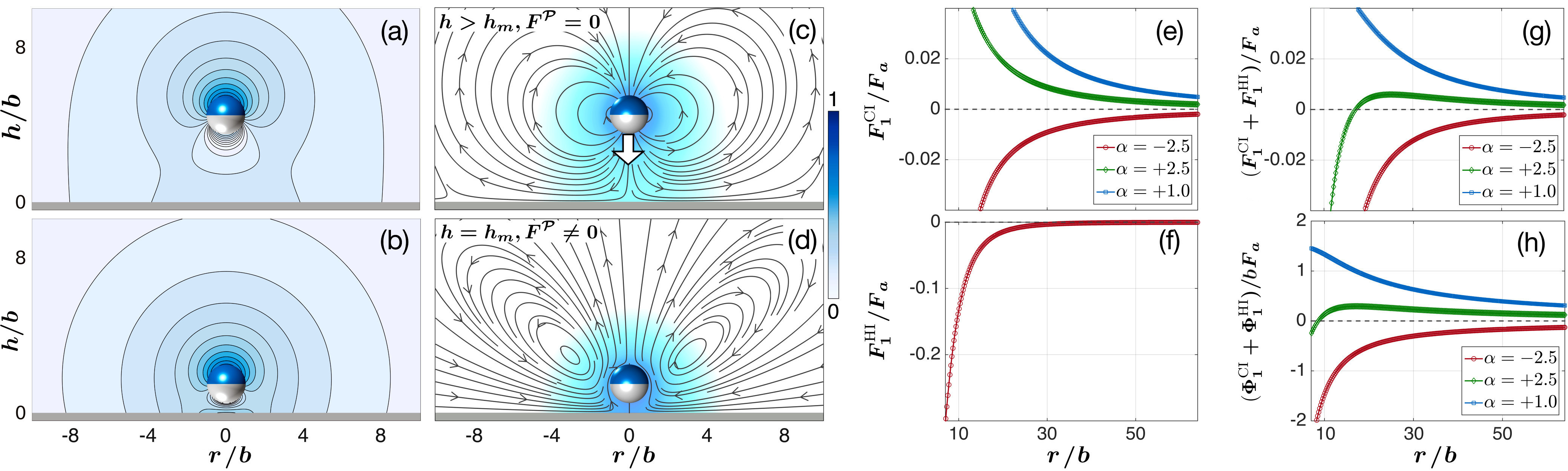
Figure 3: One and two-body dynamics of autophoretic colloids near a plane wall. Panel (a-b) are contour-maps of the chemical field around a colloid at two heights from the wall, while (c-d) are the corresponding flow streamlines overlaid on the normalized logarithm of the flow speed. Panel (e) shows the quantitative variation of planar chemical forces, while panel (f) contains the attractive hydrodynamic force and panel (g) is the sum of the forces. The corresponding autophoretic non-equilibrium potential is plotted in panel (h) for three values of dimensionless number $\alpha$. Panel (a-d) are for $\alpha=2.5$. Here $F_{a}=6\pi\eta b\,v_{s}$.

Using the above in Eq.(18) and retaining leading terms in distance gives the self-contribution to the active force to be

$$\mathbf{F}_{1}^{\mathcal{\text{self}}}=\, \gamma_{{\scriptscriptstyle\perp}}v_{s}\left(\boldsymbol{p}_{1}+\frac{b^{2}}{2\alpha h^{2}}\hat{\boldsymbol{z}}\right).$$ (25)

where

$$v_{s}=\frac{M^{(0)}J^{(\text{1})}}{16\pi^{2}b^{4}D},\qquad\alpha=\frac{J^{(1)}}{J^{(0)}},$$

are, respectively, the intrinsic self-propulsion velocity and ratio of dipolar to monopolar activity. The propulsive force is directed along or opposite to the orientation accordingly as the product $M^{(0)}J^{(1)}$ is positive or negative. For a given sign of $v_{s}$ the interaction with the wall depends only on the activity ratio. For a particle with $v_{s},\alpha>0$, forces are balanced at a height $h^{2}=b^{2}/2\alpha$, and a self-levitating state results. For other sign combinations, the particle is either repelled from or attracted to the wall. In the latter case, when the particle is brought to rest by steric interactions at a height $h_{m}$, the Stokeslet (force monopole on the colloid) on it points normal to and away from the wall. The chemical and flow fields produced by a particle at heights $h>h_{m}$ and $h=h_{m}$ are shown in Fig.( 3).

The CI force to leading order is

$$\mathbf{F}_{1}^{\text{CI}}(\boldsymbol{r},\boldsymbol{p}_{2}) =2\gamma_{{\scriptscriptstyle\parallel}}v_{s}\left(\frac{b^{2}\hat{\boldsymbol{r}}}{\alpha r^{2}}+\frac{b^{3}}{r^{3}}\left[\boldsymbol{p}_{2}-3(\boldsymbol{p}_{2}\cdot\hat{\boldsymbol{r}})\hat{\boldsymbol{r}}\right]+\frac{b^{2}\hat{\boldsymbol{r}}^{*}}{\alpha r^{*2}}+\frac{b^{3}}{r^{*3}}\left[\boldsymbol{p}_{2}-3(\boldsymbol{p}_{2}\cdot\hat{\boldsymbol{r}}^{*})\hat{\boldsymbol{r}}^{*}\right]\right),$$ (26)

with orientation-independent inverse-square and orientation-dependent inverse-cube contributions. From the expression for the force on particle $2$, obtained by interchanging indices, it is clear that the forces are non-reciprocal and violate the action-reaction principle. At a fixed height, the CI force can be expressed as the gradient, with respect to in-plane coordinates, of a non-equilibrium potential,

$$\Phi_{\text{1}}^{\text{CI}}(\boldsymbol{r},\boldsymbol{p}_{2})=2\gamma_{{\scriptscriptstyle\parallel}}bv_{s}\left(\frac{b}{\alpha r}+\frac{b}{\alpha r^{*}}-\frac{b^{2}}{r^{2}}\left[\boldsymbol{p}_{2}\cdot\hat{\boldsymbol{r}}\right]-\frac{b^{2}}{r^{*2}}\left[\boldsymbol{p}_{2}\cdot\hat{\boldsymbol{r}}^{*}\right]\right).\quad(\text{fixed height)}$$ (27)

In general, CI terms at any order can be so expressed if the friction tensors are independent of configuration. Notably, the autophoretic non-equilibrium potential is orientation-dependent, unlike the orientation-independent non-equilibrium potentials that appear in phoretic phenomena in externally imposed gradients Squires (2001); Di Leonardo et al. (2009).

The HI force has a more complicated functional form that simplifies when particle $2$ is oriented normal to the wall:

$$\mathbf{F}_{1}^{\text{HI}}(\boldsymbol{r}) =-\frac{\gamma_{{\scriptscriptstyle\parallel}}\gamma_{\perp}v_{s}}{2\pi\eta}\left(1+\frac{b^{2}}{2\alpha h^{2}}\right)\frac{3h^{3}}{(r^{2}+4h^{2})^{5/2}}\boldsymbol{r}.$$ (28)

It has an explicit dependence on the height of the particle pair from the wall. With the orientation normal to the wall, the HI force can also be expressed as the gradient, with respect to in-plane coordinates, of a non-equilibrium potential,

$$\Phi_{1}^{\text{HI}}(\boldsymbol{r})=-\frac{\gamma_{{\scriptscriptstyle\parallel}}\gamma_{\perp}v_{s}}{2\pi\eta}\left(1+\frac{b^{2}}{2\alpha h^{2}}\right)\frac{h^{3}}{(r^{2}+4h^{2})^{3/2}},\quad(\boldsymbol{p}_{2}\perp\text{wall}).$$ (29)

This follows from the irrotational character the flow assumes when particle $2$ is oriented normal to the wall. In contrast, flow in a Hele-Shaw geometry (parallel walls separated by a gap small compared to their size) is irrotational for any orientation Liron and Mochon (1976); Thutupalli et al. (2018); Kanso and Michelin (2019) and non-equilibrium hydrodynamic potentials then exist for arbitrary orientations. In general, such potentials will fail to express the HI when the flow contains significant amounts of vorticity. The CHI contains product of gradients of the Laplace and Stokes Green’s functions and, therefore, is never the gradient of a potential. However, as it has a weaker distance-dependence than both CI and HI, the potentials, when they exist, capture the leading contributions to the forces.

We plot our results for forces and potential in panels (e-h) of Fig.(3), as a function lateral pair separation $r$, at different values of $\alpha$. It should be noted that the planar chemical force, obtained from Eq.(26), contains contributions up to $O(1/r^{4})$ when it is evaluated for orientation vectors along $\hat{z}$ direction. In this setting, the next term of the chemical force contributes only at $O(1/r^{6})$, and is thus, not included for this analysis. In panel (e), we show that the chemical force $\mathbf{F}_{1}^{\text{CI}}$ depends on the sign of $\alpha$, which is controlled by the sign of $J^{(0)}$, while the hydrodynamic component $\mathbf{F}_{1}^{\text{HI}}$ is always attractive Singh and Adhikari (2016). Thus, the effective potential has a barrier if the chemical interaction is repulsive, as shown in panel (h); the effective interaction is then repulsive for $r>r_{c}$, and attractive for $r<r_{c}$ where

$$r_{c} \sim h\sqrt{\frac{3\alpha h\gamma_{\perp}}{4\pi b^{2}\eta}}.$$ (30)

is an interaction scale that depends on the height from the wall. The emergence of a length scale in slow viscous flow near a wall has also been noted in another context Driscoll et al. (2017).

We emphasize conditions in which non-equilibrium potentials exist. The CI always admits a potential when the friction tensors are constant; the HI always admits a potential when the flow is irrotational; the CHI, in general, does not admit a potential. However, as CHI is sub-dominant in comparison to CI and HI, it is not surprising that the approximation of forces by potentials leads to good agreement with simulations below, where no such approximation is made. We do not present a similarly detailed characterization of the active torque but turn, instead, to simulations of many-body effects where such torques are included.

In panel (a-l) of Fig.(4), we show the dynamics of $2^{11}$ autophoretic colloids for three different values of the activity number $\alpha$. In all cases, we start from an initially random hard-sphere configuration Skoge et al. (2006). Panels (a-d) of Fig.(4) correspond to $\alpha<1$; here the chemical repulsion dominates the hydrodynamic attraction. The result is a liquid-like steady-state as the effective interaction between the colloids is fully repulsive. For a larger value of $\alpha=2.5$, there is a barrier at $r=r_{c}$ as explained above (see Eq.(26)). This leads to arrested phase separation with clusters of particles, as shown in panels (e-h). The dynamic clusters are similar to those reported in experiments of autophoretic colloids Palacci et al. (2013); Theurkauff et al. (2012). When $\alpha$ is negative, both chemical and hydrodynamic interactions are attractive, and full phase separation is achieved. Thus, we have identified three distinct phases in the space of chemical parameters; see Fig.(4) (m). We restrict $J^{(1)}$ to positive values as it corresponds to self-propulsion into the wall, which is necessary in our model to induce the Stokeslet away from the wall, which leads to the attractive hydrodynamic forces between the colloids. The chemical monopole $J^{(0)}$, on the other hand, can take both positive and negative values. Thus, although the dynamics is determined in terms of a single ratio $\alpha$, it is useful to show the two-dimensional phase diagram of Fig.(4) (m).

The average number of particles $N_{c}$ in the arrested clusters can be tuned by varying the activity parameter $\alpha$. In panel (n) of Fig.(4), we show that $N_{c}$ is linearly proportional to $\alpha$. The scaling can be understood from the fact that the number of particles in a two-dimensional cluster is proportional to $r_{c}^{2}$, and from Eq.(30) $r_{c}$ is proportional to $\sqrt{\alpha}$. It is interesting to compare the resulting linear scaling with the experiments of Theurkauff et al. (2012); Buttinoni et al. (2013). There, the cluster size grows linearly with the self-propulsion speed $v_{s}$ of isolated colloids, when this speed is varied by adjusting the fuel concentration or light intensity. Within our theory, $v_{s}$ is indeed proportional to $\alpha$, but only if the monopole current $J^{(0)}$ is held fixed as the dipolar activity $J^{(1)}$ is varied. At present we can see no reason to expect constant $J^{(0)}$ on varying the overall fuel level, in which case the explanation of the experimental linear scaling lies beyond the present theory. However, this finding may offer valuable mechanistic information. Specifically, we assumed autophoresis to stem from the active surface chemical flux $j^{\mathcal{A}}$ of a single diffusant field $c$, whereas the mechanism of self-propulsion arising in experimental systems may instead require a description involving multiple (possibly charged) diffusant species Brown and Poon (2014); Brown et al. (2017).

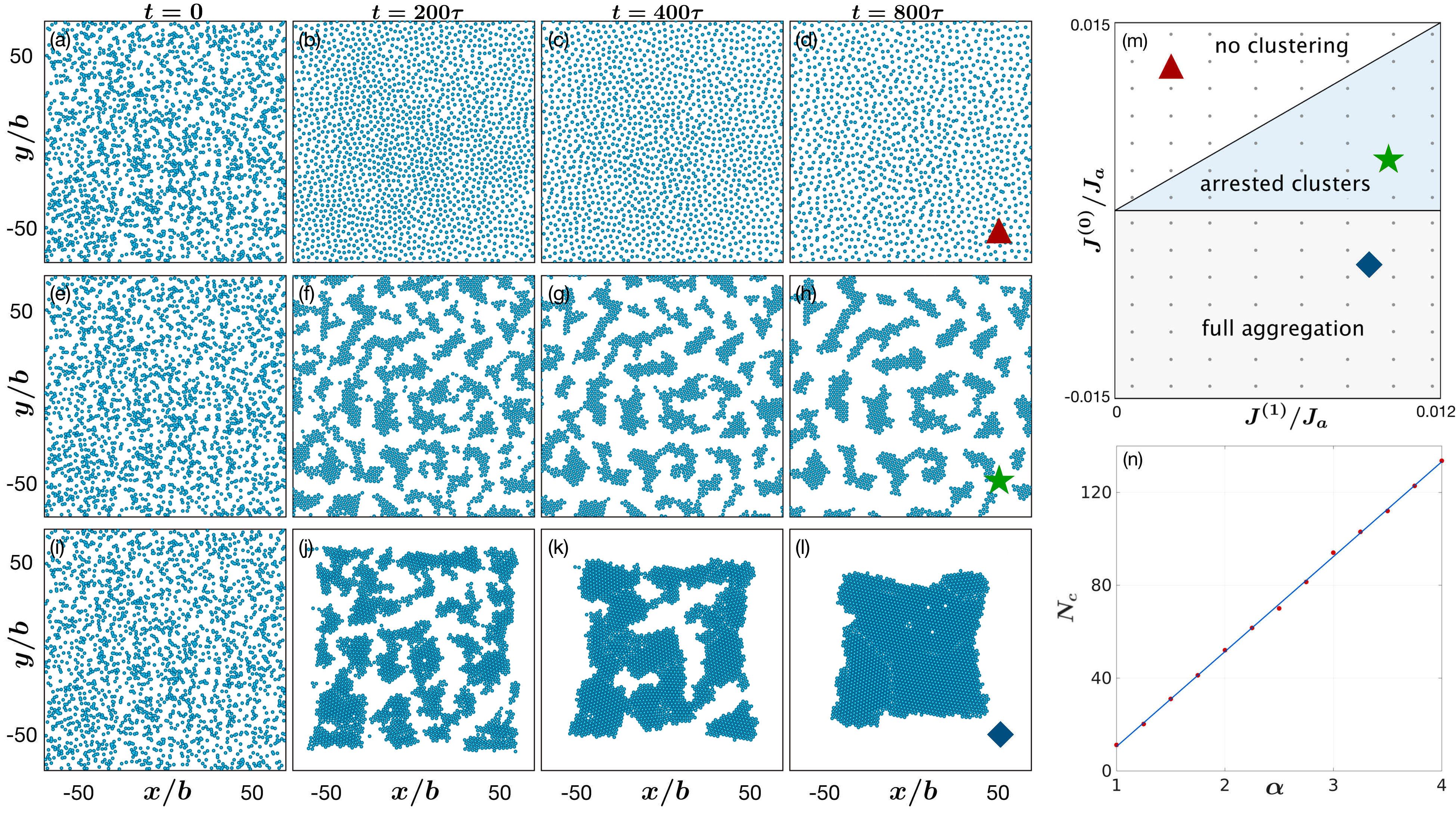
Figure 4: Self-assembly of $2^{11}$ autophoretic colloids. Panels (a-l) corresponds to three distinct states as indicated in the state diagram of panel (m), in the plane of strengths of the chemical dipole $J^{(1)}$ and monopole $J^{(0)}$ (see (16) for the model used). The gray dots denote simulation points, and $J_{a}=Db^{-2}$. Panel (n) is average number of particles in a cluster ($N_{c}$) as function of the ratio $\alpha$. Here $\tau=b/v_{s}$. We emphasize that no periodic boundary condition is used and the system is only confined by a plane infinite wall. The panels (a-l) have been cropped in the same extent of space to clearly show the difference in the three regimes.

IV Discussion

We have shown that chemical and hydrodynamic many-body effects in a suspension of autophoretic particles can be fully determined in terms of elastance, coupling and friction tensors. These tensors can be calculated from the phoretic mobility and the Green’s functions of the Laplace and Stokes equations that incorporate the appropriate boundary conditions on the chemical and the flow.

For particles at fixed heights from, and oriented normal to, a planar no-flux, no-slip wall, chemical and hydrodynamic forces can be expressed as in-plane gradients of a non-equilibrium potential. This remarkably simple pairwise description is fully underpinned by our general treatment of the many-body coupling between a rapid chemical diffusant, slip and hydrodynamic interactions, whose numerical investigation in other geometries we leave to future work. The potential can be purely attractive or repulsive, or have a barrier. Our barrier heights scale like $F_{a}b\sim 6\pi\eta b^{2}\,v_{s}$, which for a typical experiment Palacci et al. (2013), with radius $b=2$ $\mathrm{\mu m}$ and self-propulsion speed $v_{s}=10$ $\mathrm{\mu ms^{-1}}$, is roughly $10^{-19}$ J, two orders of magnitude higher than the thermal energy $k_{B}T$. This changes for smaller particles so that chemical, hydrodynamic and thermal forces are then all relevant. Our many-body formalism is generalizable to this case, and also, once they are fully identified, to some of more complex multi-species mechanisms of autophoresis that may be important experimentally.

Although we have only considered the chemical field, our formalism is applicable to any harmonic scalar field (for example, a temperature field Würger (2010)) produced locally by the colloids or due to an external gradient. In this work, we do not resolve the near-field hydrodynamic interactions between the colloids. This can be done in our theory by using lubrication-corrected friction, mobility, and propulsion tensors Singh and Adhikari (2018). While our simulations allow for orientational fluctuations, albeit of a small magnitude, the analytical form of the potential is obtained in the limit of zero orientational fluctuation. The excellent agreement between the theory and the simulation confirms that small orientational fluctuations do not significantly change the form of the potential. We leave the investigation of non-equilibrium potential, if one exists, for large orientational fluctuations to future work. In particular, when the propulsion direction of particles is not constrained to lie normal to the wall, the tangential component creates the conditions under which motility-induced phase separation Cates and Tailleur (2015) can be expected to arise. This is a separate mechanism from the one studied here which can instead be classified as flow-induced phase separation (FIPS) Singh and Adhikari (2016). The full problem presumably combines both of these types of active phase separation in a complex way. This is one reason why we have focused here on the pure FIPS limit of strongly aligned particles as the exemplary problem for combining hydrodynamic and chemical interactions in active colloidal systems.

Appendix A Boundary integrals solution for elastance tensors

The boundary integral equation of the Laplace equation gives the concentration field on the surface of the $i$-th colloid in terms of and integral over boundaries of all the colloids

$$\tfrac{1}{2}c\,(\boldsymbol{r}_{i})=\int H(\boldsymbol{R}_{i}+\mathbf{\boldsymbol{\rho}}_{i},\,\boldsymbol{R}_{k}+\mathbf{\boldsymbol{\rho}}_{k})\,j^{\mathcal{A}}(\boldsymbol{\rho}_{k})\,\text{d}S_{k}+\int L(\boldsymbol{R}_{i}+\mathbf{\boldsymbol{\rho}}_{i},\,\boldsymbol{R}_{k}+\mathbf{\boldsymbol{\rho}}_{k})\,c(\boldsymbol{\rho}_{k})\,\text{d}S_{k}.$$ (31)

Here $L=D\boldsymbol{\hat{\rho}}\cdot\mathbf{\boldsymbol{\nabla}}H$ and the integrand vanishes at any other boundary in the bulk fluid and at the infinity. We use the Galerkin method of solution by expanding the boundary fields in terms of tensorial spherical harmonics, as given in Eq.(4). The principle advantage of the Galerkin method is that the matrix elements of the linear system, which are double integrals over the particle boundaries, can be calculated exactly in terms of the Green’s functions, and thus, provides the greatest accuracy for the least number of discrete degrees of freedom Muldowney and Higdon (1995); Youngren and Acrivos (1975). Such calculations would be prohibitively expensive in the boundary element method, which instead collocates the integral equation at specific points on the boundary. Multiplying both sides of Eq.(31) by the $m$-th basis function and integrating on the surface of the i-th colloid gives a linear system for the unknown $\mathbf{C}_{i}^{(m)}$

$$\tfrac{1}{2}\mathbf{C}_{i}^{(m)}=\boldsymbol{H}_{ik}^{(m,\,m^{\prime})}(\boldsymbol{R}_{i},\boldsymbol{R}_{k})\cdot\mathbf{J}_{k}^{(m^{\prime})}+\boldsymbol{L}_{ik}^{(m,m^{\prime})}(\boldsymbol{R}_{i},\boldsymbol{R}_{k})\cdot\mathbf{C}_{k}^{(m^{\prime})}$$

Comparing with Eq.(7), the elastance tensors are given as

$$\boldsymbol{\varepsilon}{}_{ik}^{(m,m^{\prime})}=-\Big{[}\big{(}\tfrac{1}{2}\boldsymbol{I}-\boldsymbol{L}\big{)}^{-1}\boldsymbol{H}\Big{]}_{ik}^{(m,m^{\prime})}.$$ (32)

Here $\boldsymbol{H}$ and $\boldsymbol{L}$ are matrices, whose $(m,\,m^{\prime})$ element in the $ik$ block are $\boldsymbol{H}_{ik}^{(m,\,m^{\prime})}(\boldsymbol{R}_{i},\boldsymbol{R}_{k})$ and $\boldsymbol{L}_{ik}^{(m,\,m^{\prime})}(\boldsymbol{R}_{i},\boldsymbol{R}_{k})$ respectively. The matrix elements of the linear system are

$$\boldsymbol{H}_{ik}^{(m,m^{\prime})}(\boldsymbol{R}_{i},\boldsymbol{R}_{k})=\tilde{w}_{m}\tilde{w}_{m^{\prime}} \int\mathbf{Y}^{(m)}(\hat{\bm{\rho}}_{i})H(\boldsymbol{R}_{i}+\bm{\rho}_{i},\boldsymbol{R}_{k}+\bm{\rho}_{k})\mathbf{Y}^{(m^{\prime})}(\hat{\bm{\rho}}_{k})\,d\text{S}_{i}d\text{S}_{k},$$

$$\boldsymbol{L}_{ik}^{(m,m^{\prime})}(\boldsymbol{R}_{i},\boldsymbol{R}_{k})=\tilde{w}_{m}w_{m^{\prime}} \int\mathbf{Y}^{(m)}(\hat{\bm{\rho}}_{i})L(\boldsymbol{R}_{i}+\bm{\rho}_{i},\boldsymbol{R}_{k}+\bm{\rho}_{k})\mathbf{Y}^{(m^{\prime})}(\hat{\bm{\rho}}_{k})d\text{S}_{i}d\text{S}_{k}.$$

The above integrals are completed by Taylor expansion of the Green’s function and using the orthogonality of the basis functions ($w_{m}\tilde{w}_{m^{\prime}}\int\mathbf{Y}^{(m)}(\hat{\bm{\rho}}_{i})\mathbf{Y}^{(m^{\prime})}(\hat{\bm{\rho}}_{i})\,d\text{S}_{i}=\delta_{mm^{\prime}}\boldsymbol{\Delta}$) and standard Bessel integrals to obtain Singh et al. (2015)

$$\boldsymbol{H}_{ik}^{(m,m^{\prime})}(\boldsymbol{R}_{i},\boldsymbol{R}_{k}) =\begin{cases}\frac{\delta_{ik}\delta_{mm^{\prime}}}{4\pi bDw_{m}}\mathbf{\Delta}^{(m)}&{\displaystyle k=i,}\\ {\displaystyle b^{m+m^{\prime}}\bm{\nabla}_{{\scriptscriptstyle\boldsymbol{R}_{i}}}^{m}\bm{\nabla}_{{\scriptscriptstyle\boldsymbol{R}_{k}}}^{m^{\prime}}H(\boldsymbol{R}_{i},\boldsymbol{R}_{k})}&{\displaystyle k\neq i,}\end{cases}$$

$$\boldsymbol{L}_{ik}^{(m,m^{\prime})}(\boldsymbol{R}_{i},\boldsymbol{R}_{k}) =\begin{cases}-\frac{1}{2}\mathbf{\Delta}^{(m)}\qquad&{\displaystyle k=i,}\\ e_{m}\bm{\nabla}_{{\scriptscriptstyle\boldsymbol{R}_{i}}}^{m}\bm{\nabla}_{{\scriptscriptstyle\boldsymbol{R}_{k}}}^{m^{\prime}}H(\boldsymbol{R}_{i},\boldsymbol{R}_{k})\quad\,\,&{\displaystyle k\neq i.}\end{cases}$$

Here $e_{m}=w_{m-1}Db^{(m+m^{\prime}-5)}/(4\pi\tilde{w}_{m}\tilde{w}_{m-1})$ and $\mathbf{\Delta}^{(m)}$ is a tensor of rank $2m$, which reduces a tensor of rank $m$ to its symmetric irreducible form.

With the matrix elements so determined, the linear system can be solved by a variety of methods. Here, we use the venerable “method of reflections” due to Smoluchowski, which is the Jacobi iteration in disguise. The solution after the $n$-th iteration is Saad (2003)

$$\Big{(}\boldsymbol{\varepsilon}_{ik}^{(m,m^{\prime})}\Big{)}^{[n]} =-\frac{1}{\mathit{A}_{ii}^{(m,m)}}\bigg{[}\boldsymbol{H}_{ik}^{(m,m^{\prime})}-\boldsymbol{\sum^{\prime}}\boldsymbol{A}_{ij}^{(m,m^{\prime\prime})}\cdot\Big{(}\boldsymbol{\boldsymbol{\varepsilon}}_{jk}^{(m^{\prime\prime},m^{\prime})}\Big{)}^{[n-1]}\bigg{]}.$$ (34)

Here $\boldsymbol{A}_{ik}^{(m,m^{\prime})}=\tfrac{1}{2}\boldsymbol{I}_{ik}^{(m,m^{\prime})}-\boldsymbol{L}_{ik}^{(m,m^{\prime})}$, and the primed summation in Eq.(34) indicates that the diagonal term ($i=j=k$ and $m=m^{\prime}=m^{\prime\prime}$) is excluded Saad (2003). To start the iteration, we use the one-body solution of the linear system,

$$\Big{(}\boldsymbol{\varepsilon}{}_{ik}^{(m,m^{\prime})}\Big{)}^{[0]}=\delta_{ik}\delta_{mm^{\prime}}\varepsilon_{ii}^{(l)}=\frac{\delta_{ik}\delta_{mm^{\prime}}}{4\pi bDw_{m}}\mathbf{\Delta}^{(m)}.$$

Chemical interactions, given by the off-diagonal ($i\neq j$) elastance tensors, appear at the second iteration,

$$\Big{(}\boldsymbol{\varepsilon}_{ik}^{(m,m^{\prime})}\Big{)}^{[1]} =-b^{m+m^{\prime}}\bm{\nabla}_{{\scriptscriptstyle\boldsymbol{R}_{i}}}^{m}\bm{\nabla}_{{\scriptscriptstyle\boldsymbol{R}_{k}}}^{m^{\prime}}H(\boldsymbol{R}_{i},\boldsymbol{R}_{k}).$$

The solution of the elastance tensors at the third iteration is

$$\Big{(}\boldsymbol{\varepsilon}_{ik}^{(m,m^{\prime})}\Big{)}^{[2]} =\Big{(}\boldsymbol{\varepsilon}_{ik}^{(m,m^{\prime})}\Big{)}^{[1]}+\boldsymbol{\sum^{\prime}}\Big{[}-\tfrac{4\pi Db^{2m+2m^{\prime}-1}}{(m^{\prime}-1)!(2m^{\prime}+1)!!}\bm{\nabla}_{{\scriptscriptstyle\boldsymbol{R}_{i}}}^{m}\bm{\nabla}_{{\scriptscriptstyle\boldsymbol{R}_{j}}}^{m^{\prime}}H(\boldsymbol{R}_{i},\boldsymbol{R}_{j})\Big{]}\bm{\nabla}_{{\scriptscriptstyle\boldsymbol{R}_{j}}}^{m}\bm{\nabla}_{{\scriptscriptstyle\boldsymbol{R}_{k}}}^{m^{\prime}}H(\boldsymbol{R}_{j},\boldsymbol{R}_{k}).$$

The above recipe can then used to be used to systematically obtain the elastance tensors at all orders. The higher order Jacobi solutions are obtained in terms of higher gradients of the Green’s function, and are thus, subleading to the lower order solutions. In this work, we have used the solution of the elastance tensor at the second iteration. The coupling tensors of Eq.(11) satisfy

$$\mathbb{\boldsymbol{\chi}}^{(l,m)}=-\frac{\tilde{w}_{l-1}w_{m}}{bw_{l+m-2}}\mathbf{M}_{i}^{(l+m-2)}\boldsymbol{I}+\frac{\tilde{w}_{l-1}w_{m}}{bw_{l+m}}\mathbf{M}_{i}^{(l+m)},$$

where the first term is non-vanishing for $l+m-2\geq 0$, and $\mathbf{M}_{i}^{(m)}=w_{l}\int\mu_{c}(\boldsymbol{R}_{i}+\boldsymbol{\rho}_{i})\mathbf{Y}^{(m)}(\boldsymbol{\rho}_{i})\,dS_{i}$ are tensorial spherical harmonic coefficients of phoretic mobility.

Appendix B Simulation Details

With vanishing inertia, Newton’s equations Eq.(14) can be inverted to obtain the rigid body motion of active colloids in terms of known quantities:

$$\mathbf{V}_{i} =\boldsymbol{\mu}_{ik}^{TT}\cdot\mathbf{F}_{k}^{\mathcal{P}}+\boldsymbol{\mu}_{ik}^{TR}\cdot\mathbf{T}_{k}^{\mathcal{P}}+\boldsymbol{\pi}_{ij}^{(T,l)}\cdot\negmedspace\boldsymbol{\chi}^{(l,m^{\prime})}\negmedspace\cdot\boldsymbol{\varepsilon}{}_{jk}^{(m^{\prime},m)}\cdot\mathbf{J}{}_{k}^{(m)},$$ (35a)

$$\boldsymbol{\Omega}_{i} =\boldsymbol{\mu}_{ik}^{RT}\cdot\mathbf{F}_{k}^{\mathcal{P}}+\boldsymbol{\mu}_{ik}^{RR}\cdot\mathbf{T}_{k}^{\mathcal{P}}+\boldsymbol{\pi}_{ij}^{(T,l)}\cdot\negmedspace\boldsymbol{\chi}^{(l,m^{\prime})}\negmedspace\cdot\boldsymbol{\varepsilon}{}_{jk}^{(m^{\prime},m)}\cdot\mathbf{J}{}_{k}^{(m)}.$$ (35b)

Here the propulsion tensors $\boldsymbol{\pi}^{(\alpha,l^{\prime}\sigma^{\prime})}$ give active contributions due to the slip Singh et al. (2015) and the mobility matrices $\boldsymbol{\mu}^{\alpha\beta}$, with $(\alpha,\beta)=(T,R)$ give passive hydrodynamic interactions Mazur and Saarloos (1982); Ladd (1988). The above dynamical system, in simulations, is truncated at $l=3$ and integrated numerically using the open-source PyStokes library Singh et al. (2014) with an initial condition of random packing of hard-spheres Skoge et al. (2006). We then study the system near a plane wall by computing the mobility, propulsion and elastance tensors using the Green’s function of sec III. Our system is only confined by a plane wall and there is no periodic boundary condition. Thus, it is a distinctive feature of the present approach to colloid hydrodynamics that a finite number of colloids in an infinite expanse of fluid can be simulated, without having to either truncate the size of the system or impose periodic boundary condition.

The orientations of the colloids are stabilized along the wall normal by external torques $\mathbf{T}^{\mathcal{P}}=T_{0}(\mathbf{\hat{z}}\times\boldsymbol{p}_{i})$. The number of colloids $N$, for respective plots, are: Fig.3(a-d): $N=1$; Fig.3(e-f): $N=2$; Fig.4: $N=2^{11}$. Other parameters used in the simulations are: radius of colloids ($b=1$), strength of the chemical monopole ($J_{0}^{(0)}=4$), strength of the chemical dipole ($J^{(1)}=10$), the strength of the bottom-heaviness ($T_{0}=0.2$), diffusion constant ($D=1000$), and dynamic viscosity ($\eta=1$). We vary the ratio $\alpha=J^{(1)}/J_{0}^{(0)}$ in Fig.4(n) to map the state diagram. The conservative inter-particle force $\mathbf{F}_{i}^{\mathcal{P}}=-\boldsymbol{\nabla}_{{\scriptscriptstyle\mathbf{R}_{i}}}U$ is due to a short-ranged repulsive potential $U(r)=\epsilon\left(\frac{r_{min}}{r}\right)^{12}-2\epsilon\left(\frac{r_{min}}{r}\right)^{6}+\epsilon,$ for $r<r_{min}$ and zero otherwise Weeks et al. (1971), where $\epsilon$ is the potential strength. The WCA parameters for particle-particle repulsion are: $r_{min}=4.4,\,\epsilon=0.04$, while for the particle-wall repulsion we choose $r_{min}=3,\,\epsilon=0.08$.

References

- Brennen and Winet (1977) C. Brennen and H. Winet, “Fluid mechanics of propulsion by cilia and flagella,” Annu. Rev. Fluid Mech. 9, 339–398 (1977).
- Anderson (1989) J. L. Anderson, “Colloid transport by interfacial forces,” Annu. Rev. Fluid Mech. 21, 61–99 (1989).
- Ebbens and Howse (2010) S. J. Ebbens and J. R. Howse, “In pursuit of propulsion at the nanoscale,” Soft Matter 6, 726–738 (2010).
- Singh et al. (2015) R. Singh, S. Ghose, and R. Adhikari, “Many-body microhydrodynamics of colloidal particles with active boundary layers,” J. Stat. Mech 2015, P06017 (2015).
- Singh and Adhikari (2016) R. Singh and R. Adhikari, “Universal hydrodynamic mechanisms for crystallization in active colloidal suspensions,” Phys. Rev. Lett. 117, 228002 (2016).
- Singh and Adhikari (2018) R. Singh and R. Adhikari, “Generalized Stokes laws for active colloids and their applications,” J. Phys. Commun. 2, 025025 (2018).
- Thutupalli et al. (2018) S. Thutupalli, D. Geyer, R. Singh, R. Adhikari, and H. A. Stone, “Flow-induced phase separation of active particles is controlled by boundary conditions,” Proc. Natl. Acad. Sci. 115, 5403–5408 (2018).
- Goldstein (2015) R. E. Goldstein, “Green algae as model organisms for biological fluid dynamics,” Ann. Rev. Fluid Mech. 47, 343–375 (2015).
- Pedley (2016) T. J. Pedley, “Spherical squirmers: models for swimming micro-organisms,” IMA J. Appl. Math. 81, 488–521 (2016).
- Petroff et al. (2015) A. P. Petroff, X.-L. Wu, and A. Libchaber, “Fast-moving bacteria self-organize into active two-dimensional crystals of rotating cells,” Phys. Rev. Lett. 114, 158102 (2015).
- Palacci et al. (2013) J. Palacci, S. Sacanna, A. P. Steinberg, D. J. Pine, and P. M. Chaikin, “Living crystals of light-activated colloidal surfers,” Science 339, 936–940 (2013).
- Theurkauff et al. (2012) I. Theurkauff, C. Cottin-Bizonne, J. Palacci, C. Ybert, and L. Bocquet, “Dynamic clustering in active colloidal suspensions with chemical signaling,” Phys. Rev. Lett. 108, 268303 (2012).
- Buttinoni et al. (2013) I. Buttinoni, J. Bialké, F. Kümmel, H. Löwen, C. Bechinger, and T. Speck, “Dynamical clustering and phase separation in suspensions of self-propelled colloidal particles,” Phys. Rev. Lett. 110, 238301 (2013).
- Pohl and Stark (2014) O. Pohl and H. Stark, “Dynamic clustering and chemotactic collapse of self-phoretic active particles,” Phys. Rev. Lett. 112, 238303 (2014).
- Saha et al. (2014) S. Saha, R. Golestanian, and S. Ramaswamy, “Clusters, asters, and collective oscillations in chemotactic colloids,” Phys. Rev. E 89, 062316 (2014).
- Liebchen et al. (2017) B. Liebchen, D. Marenduzzo, and M. E. Cates, “Phoretic interactions generically induce dynamic clusters and wave patterns in active colloids,” Phys. Rev. Lett. 118, 268001 (2017).
- Yan and Brady (2016) W. Yan and J. F. Brady, “The behavior of active diffusiophoretic suspensions: An accelerated laplacian dynamics study,” J. Chem. Phys. 145, 134902 (2016).
- Liebchen and Löwen (2018) B. Liebchen and H. Löwen, “Which interactions dominate in active colloids?” arXiv preprint arXiv:1808.07389 (2018).
- Popescu et al. (2018) M. N. Popescu, W. E. Uspal, Z. Eskandari, M. Tasinkevych, and S. Dietrich, “Effective squirmer models for self-phoretic chemically active spherical colloids,” Eur. Phys. J. E 41, 145 (2018).
- Liebchen et al. (2015) B. Liebchen, D. Marenduzzo, I. Pagonabarraga, and M. E. Cates, “Clustering and pattern formation in chemorepulsive active colloids,” Phys. Rev. Lett. 115, 258301 (2015).
- Soto and Golestanian (2014) R. Soto and R. Golestanian, “Self-assembly of catalytically active colloidal molecules: tailoring activity through surface chemistry,” Phys. Rev. Lett. 112, 068301 (2014).
- Hess (2015) S. Hess, Tensors for physics (Springer, 2015).
- Maxwell (1873) J. C. Maxwell, A treatise on electricity and magnetism, Vol. 1 (Clarendon press, Oxford, 1873) p. 89.
- Ghose and Adhikari (2014) S. Ghose and R. Adhikari, “Irreducible representations of oscillatory and swirling flows in active soft matter,” Phys. Rev. Lett. 112, 118102 (2014).
- Mazur and Saarloos (1982) P. Mazur and W. van Saarloos, “Many-sphere hydrodynamic interactions and mobilities in a suspension,” Physica A: Stat. Mech. Appl. 115, 21–57 (1982).
- Ladd (1988) A. J. C. Ladd, “Hydrodynamic interactions in a suspension of spherical particles,” J. Chem. Phys. 88, 5051–5063 (1988).
- Lorentz (1896) H. A. Lorentz, “A general theorem concerning the motion of a viscous fluid and a few consequences derived from it,” Versl. Konigl. Akad. Wetensch. Amst 5, 168–175 (1896).
- Blake (1971) J. R. Blake, “A note on the image system for a Stokeslet in a no-slip boundary,” Proc. Camb. Phil. Soc. 70, 303–310 (1971).
- Kim and Karrila (1991) S. Kim and S. J. Karrila, Microhydrodynamics: Principles and Selected Applications (Butterworth-Heinemann, Boston, 1991).
- Squires (2001) T. M. Squires, “Effective pseudo-potentials of hydrodynamic origin,” J. Fluid Mech. 443, 403–412 (2001).
- Di Leonardo et al. (2009) R Di Leonardo, F Ianni, and G Ruocco, “Colloidal attraction induced by a temperature gradient,” Langmuir 25, 4247–4250 (2009).
- Liron and Mochon (1976) N. Liron and S. Mochon, “Stokes flow for a Stokeslet between two parallel flat plates,” J. Eng. Math. 10, 287–303 (1976).
- Kanso and Michelin (2019) E. Kanso and S. Michelin, “Phoretic and hydrodynamic interactions of weakly confined autophoretic particles,” J. Chem. Phys. 150, 044902 (2019).
- Driscoll et al. (2017) M. Driscoll, B. Delmotte, M. Youssef, S. Sacanna, A. Donev, and P. Chaikin, “Unstable fronts and motile structures formed by microrollers,” Nat. Phys. 13, 375 (2017).
- Skoge et al. (2006) M. Skoge, A. Donev, F. H. Stillinger, and S. Torquato, “Packing hyperspheres in high-dimensional Euclidean spaces,” Phys. Rev. E 74, 041127 (2006).
- Brown and Poon (2014) A. Brown and W. Poon, “Ionic effects in self-propelled pt-coated janus swimmers,” Soft matter 10, 4016–4027 (2014).
- Brown et al. (2017) A. T. Brown, W. C. K. Poon, C. Holm, and J. de Graaf, “Ionic screening and dissociation are crucial for understanding chemical self-propulsion in polar solvents,” Soft Matter 13, 1200–1222 (2017).
- Würger (2010) A. Würger, “Thermal non-equilibrium transport in colloids,” Rep. Prog. Phys. 73, 126601 (2010).
- Cates and Tailleur (2015) M. E. Cates and J. Tailleur, “Motility-induced phase separation,” Annu. Rev. Condens. Mat. Phys. 6, 219–244 (2015).
- Muldowney and Higdon (1995) G. P. Muldowney and J. J. L. Higdon, “A spectral boundary element approach to three-dimensional Stokes flow,” J. Fluid Mech. 298, 167–192 (1995).
- Youngren and Acrivos (1975) G. Youngren and A. Acrivos, “Stokes flow past a particle of arbitrary shape: a numerical method of solution,” J. Fluid Mech. 69, 377–403 (1975).
- Saad (2003) Y. Saad, Iterative methods for sparse linear systems (SIAM, 2003).
- Singh et al. (2014) R. Singh, A. Laskar, R. Singh, and R. Adhikari, “PyStokes: Hampi,” https://github.com/rajeshrinet/pystokes/ (2014).
- Weeks et al. (1971) J. D. Weeks, D. Chandler, and H. C. Andersen, “Role of repulsive forces in determining the equilibrium structure of simple liquids,” J. Chem. Phys. 54, 5237–5247 (1971).