Reciprocal and Positive Real Balanced Truncations for Model Order Reduction of Descriptor Systems

Abstract

Model order reduction algorithms for large-scale descriptor systems are proposed using balanced truncation, in which symmetry or block skew symmetry (reciprocity) and the positive realness of the original transfer matrix are preserved. Two approaches based on standard and generalized algebraic Riccati equations are proposed. To accelerate the algorithms, a fast Riccati solver, RADI (alternating directions implicit [ADI]-type iteration for Riccati equations), is also introduced. As a result, the proposed methods are general and efficient as a model order reduction algorithm for descriptor systems associated with electrical circuit networks.

1 Introduction

Consider the following linear time invariant system:

$$E_{0}\frac{dx(t)}{dt} = A_{0}x(t)+B_{0}u(t),\quad z(t)=C_{0}x(t),$$ (1)

where $E_{0}\in\mathbb{R}^{n,n},A_{0}\in\mathbb{R}^{n,n},B_{0}\in\mathbb{R}^{n,m},C_{0}\in\mathbb{R}^{m,n}$, $x(t)\in\mathbb{R}^{n}$ is the state, $u(t)\in\mathbb{R}^{m}$ is the input, and $z(t)\in\mathbb{R}^{m}$ is the output. This is referred to as a descriptor system in the control community. The form of (1) is typical for linear passive electrical circuits in which coefficient matrices $E_{0}$ and $A_{0}$ are symmetric and transfer matrix $H(s)=C_{0}\left(sE_{0}-A_{0}\right)^{-1}B_{0}$ is symmetric or block skew symmetric. The symmetric or block skew symmetric property of the transfer matrix is referred to as reciprocity in circuit theory. The transfer matrix $H(s)$ is assumed to be positive real, whose property is referred to as passivity. Furthermore, matrix $E_{0}$ is assumed to be singular, which is also typical for linear electrical networks.

Interconnect networks in integrated circuits, packages, and printed circuit boards are mathematically described by a descriptor system. Then, the system becomes extremely large scale, which effectively prohibits simulation of the interconnect networks combined with other circuit blocks, which is necessary for design of the electronics system including the integrated circuits, packages, and printed circuit boards. Therefore, the descriptor system should be of a small size without losing behavior from zero to a specified frequency. Model order reduction (MOR) methods fulfill these requirements, and Krylov subspace methods [1], [8], [9], [10] are powerful MOR methods that can provide an accurate reduced-order model for a problem; however, these methods cannot guarantee stability when connected to other linear networks. Several methods [4], [21] are also based on the Krylov subspace, in which coefficient matrices $E_{0}$ and $A_{0}$ of (1) are written in block skew symmetric form to guarantee passivity; however, reciprocity is not guaranteed. If the coefficient matrices are written in symmetric form, reciprocity is guaranteed but passivity is not. Therefore, passivity and reciprocity are not simultaneously satisfied with Krylov subspace methods.

Positive real balanced truncation (PRBT) [22], [26] is more accurate than Krylov subspace methods, especially at high frequencies. PRBT is an extension of balanced truncation [20] in which algebraic Riccati equations (AREs) are solved. Passivity-preserving balanced truncation for electrical circuits (PABTEC) [24] provides a passive and reciprocal reduced-order model in which generalized AREs (GAREs) are solved by the Newton method with Cholesky factorized alternating direction implicit iteration to solve Lyapunov equations [6]. Note that PABTEC is applicable to index-1 and index-2 descriptor systems. Although reciprocity is guaranteed by preserving the block skew symmetry of the transfer matrix, symmetric cases are not considered in PABTEC.

Thus, in this paper, we present reciprocal and positive real balanced truncations (RPRBTs), in which reciprocity is guaranteed for symmetric and block skew symmetric cases for index-1 and index-2 systems. Moreover, a fast Riccati solver, i.e., RADI [5], is introduced. RADI solves the following ARE:

$$A^{T}X+XA+XBB^{T}X+C^{T}C=0,$$ (2)

where $A\in\mathbb{R}^{p,p},B\in\mathbb{R}^{p,m}$, and $C\in\mathbb{R}^{m,p}$. RADI provides an ARE solution that is equivalent to solutions obtained by three seemingly different methods [2], [18], [26]. In addition, RADI is the fastest among these methods. Furthermore, RADI can be applied to solving the following GARE:

$$A^{T}XE+E^{T}XA+E^{T}XBB^{T}XE+C^{T}C=0,$$ (3)

where $E\in\mathbb{R}^{n,n},A\in\mathbb{R}^{n,n},B\in\mathbb{R}^{n,m}$, and $C\in\mathbb{R}^{m,n}$. Thus, we present two methods based on an ARE or GARE that are applicable to both index-1 and index-2 systems.

RADI provides an accurate ARE solution in which Ritz values are used as the shift parameters [7]. However, it has been suggested [25] that Ritz values are insufficient for low-frequency accurate PRBT with quadratic ADI (QADI) [26], which is one of the three methods equivalent to RADI. To improve accuracy at low frequencies, which is important for electrical circuit simulations, a small negative constant value is used together with complex Ritz values as a shift in QADI. Furthermore, we extend the discussion to provide useful shift selections to generate low-frequency accurate reduced-order models using RADI.

The remainder of this paper is organized as follows. In Section 2, we provide definitions of reciprocity for index-1 and index-2 descriptor systems. In Section 3, RPRBT for an index-1 system is provided based on the ARE. In Section 4, RPRBT for index-1 and index-2 systems is provided based on the GARE, and RPRBT for the index-2 system is also provided based on the ARE. In Section 5, the shift selections of RADI are obtained to solve the ARE and GARE. We give numerical examples in Section 6 to demonstrate the effectiveness of the proposed method. Finally, conclusions are presented in Section 7.

The following notations are used in this paper. $A^{-1}$, $A^{T}$, and $A^{*}$ represent the inverse, transpose, and conjugate transpose of matrix $A$, respectively.

2 Reciprocity

Reciprocity is a fundamental principle of linear passive networks. In passive reduced-order interconnect macromodeling algorithm (PRIMA) [21], the coefficient matrices $E_{0}$ and $A_{0}$ are written in block skew symmetric form to guarantee the positive realness of the transfer function. As positive realness is guaranteed by solving the Lur’e equation or an ARE in PRBT, we do not need to write the descriptor system in block skew symmetric form. Therefore, matrices $E_{0}$ and $A_{0}$ are written in symmetric form. The coefficient matrices of (1) are expressed as follows for the impedance matrix:

$$\begin{aligned} E_{0}&=\left[\begin{array}[]{cc}A_{\mathcal{C}}{\mathcal{C}}A_{\mathcal{C}}^{T}&0\\ 0&-{\mathcal{L}}\\ \end{array}\right],\quad A_{0}=\left[\begin{array}[]{cc}-A_{\mathcal{G}}{\mathcal{G}}A_{\mathcal{G}}^{T}&-A_{\mathcal{L}}\\ -A_{\mathcal{L}}^{T}&0\end{array}\right],\\ B_{0}&=\left[\begin{array}[]{c}-A_{\mathcal{I}}\\ 0\end{array}\right],\quad C_{0}=B_{0}^{T},\end{aligned}$$ (4)

as follows for the admittance matrix:

$$\begin{aligned} E_{0}&=\left[\begin{array}[]{ccc}A_{\mathcal{C}}{\mathcal{C}}A_{\mathcal{C}}^{T}&0&0\\ 0&-{\mathcal{L}}&0\\ 0&0&0\\ \end{array}\right],\quad A_{0}=\left[\begin{array}[]{ccc}-A_{\mathcal{G}}{\mathcal{G}}A_{\mathcal{G}}^{T}&-A_{\mathcal{L}}&-A_{\mathcal{V}}\\ -A_{\mathcal{L}}^{T}&0&0\\ -A_{\mathcal{V}}^{T}&0&0\\ \end{array}\right],\\ B_{0}&=\left[\begin{array}[]{c}0\\ 0\\ I_{m}\\ \end{array}\right],\quad C_{0}=\left[\begin{array}[]{ccc}0&0&-I_{m}\\ \end{array}\right],\end{aligned}$$ (5)

and as follows for the hybrid matrix:

$$\begin{aligned} E_{0}&=\left[\begin{array}[]{ccc}A_{\mathcal{C}}{\mathcal{C}}A_{\mathcal{C}}^{T}&0&0\\ 0&-{\mathcal{L}}&0\\ 0&0&0\\ \end{array}\right],\quad A_{0}=\left[\begin{array}[]{ccc}-A_{\mathcal{G}}{\mathcal{G}}A_{\mathcal{G}}^{T}&-A_{\mathcal{L}}&-A_{\mathcal{V}}\\ -A_{\mathcal{L}}^{T}&0&0\\ -A_{\mathcal{V}}^{T}&0&0\\ \end{array}\right],\\ B_{0}&=\left[\begin{array}[]{cc}-A_{\mathcal{I}}&0\\ 0&0\\ 0&I_{m/2}\\ \end{array}\right],\quad C_{0}=\left[\begin{array}[]{ccc}-A_{\mathcal{I}}&0&0\\ 0&0&-I_{m/2}\\ \end{array}\right].\end{aligned}$$ (6)

In (4)-(6), ${\mathcal{G}}$, ${\mathcal{L}}$, and ${\mathcal{C}}$ are the conductance, inductance, and capacitance matrices, respectively. In addition, $A_{\mathcal{G}}$, $A_{\mathcal{C}}$, $A_{\mathcal{L}}$, $A_{\mathcal{I}}$, and $A_{\mathcal{V}}$ are the incidence matrices to conductors, capacitors, inductors, and independent current and voltage sources, respectively. Here, $I_{m}$ is an $m\times m$ identity matrix. Then, linear passive RLC networks satisfy the following theorem.

Theorem 1.

The linear passive networks expressed by (1) are reciprocal.

Proof. It is trivial that the transfer matrix associated with impedance and admittance are symmetric. Thus, the hybrid matrix is proved to be block skew symmetric. The hybrid matrix $H(s)$ is given as follows:

$$\begin{aligned} H(s)&=I^{\circ}_{m}B_{0}^{T}\left(sE_{0}-A_{0}\right)^{-1}B_{0}=\left[\begin{array}[]{cc}H_{11}&H_{12}\\ H_{21}&H_{22}\end{array}\right],\end{aligned}$$ (7)

where

$$I^{\circ}_{m} = \left[\begin{array}[]{cc}I_{m/2}&0\\ 0&-I_{m/2}\end{array}\right].$$

As $B_{0}^{T}\left(sE_{0}-A_{0}\right)^{-1}B_{0}$ is symmetric, $H_{11}=H_{11}^{T}$, $H_{22}=H_{22}^{T}$, and $H_{12}=-H_{21}^{T}$.
                                                                                                            

The goal of this paper is to provide reduced-order models that preserve the positive realness and symmetry or block skew symmetry of the transfer matrix. To apply RPRBT, the descriptor system of (1) must be converted to a state equation. As the first step to obtain the state equation, consider the following Weierstrass canonical form:

$$\begin{aligned} E_{0}&=T_{l}\left[\begin{array}[]{cc}I_{q}&0\\ 0&N\end{array}\right]T_{r},\quad A_{0}=T_{l}\left[\begin{array}[]{cc}J&0\\ 0&I_{n-q}\end{array}\right]T_{r},\\ \end{aligned}$$ (9)

where $J$ is the Jordan form whose eigenvalues correspond to the finite eigenvalues of the generalized eigenvalue problem $\left(E,A\right)$, whereas $N$ is a nilpotent whose eigenvalues are zero. When $N^{\mu}=0$, $N^{\mu^{\prime}}\neq 0$, and $\mu^{\prime}=\mu+1$, $\mu$ is referred to as the index. For RLC networks, the index is at most two [22].

With the Weierstrass canonical form (9), the relationships $C_{0}T_{r}^{-1}=[C_{p}~{}C_{\infty}]$ and $T_{l}^{-1}B_{0}=[B_{p}^{T}~{}B_{\infty}^{T}]^{T}$ are defined. Then, transfer matrix $G(s)$ is obtained as follows:

$$\begin{aligned} G(s)&=C_{0}\left(sE_{0}-A_{0}\right)^{-1}B_{0}\\ &=\left[\begin{array}[]{cc}C_{p}&C_{\infty}\end{array}\right]\left[\begin{array}[]{cc}\left(sI_{q}-J\right)^{-1}&\\ &\left(sN-I_{n-q}\right)^{-1}\end{array}\right]\left[\begin{array}[]{c}B_{p}\\ B_{\infty}\end{array}\right]\\ &=C_{p}\left(sI_{q}-J\right)^{-1}B_{p}+M_{0}+sM_{1},\end{aligned}$$ (10)

where $M_{0}=-C_{\infty}B_{\infty}$ and $M_{1}=-C_{\infty}NB_{\infty}$ are positive semidefinite [22]. The terms $C_{p}\left(sI_{q}-J\right)^{-1}B_{p}+M_{0}$ in (10) are the proper part of transfer matrix $G(s)$. Note that $M_{1}$ becomes a zero matrix for an index-1 system.

3 RPRBT for Index-1 Systems

The descriptor system (1) is expressed in a singular-value decomposition (SVD) canonical form for conversion to a state equation. Although SVD is necessary, it is computationally expensive for a large system. Thus, rather than SVD, we use LDL factorization, which is Cholesky-like factorization for semidefinite case: $P^{T}\alpha P=LDL^{T}$, where $\alpha$ is symmetric, $P$ is a permutation, $L$ is a lower triangular matrix, and $D$ is a diagonal matrix of rank less than full rank. By applying LDL factorization to $A_{\mathcal{C}}\mathcal{C}A_{\mathcal{C}}$ and ${\mathcal{L}}$ in (4)-(6), matrix $E_{0}$ can be expressed as follows:

$$\begin{aligned} E_{0}&=V\left[\begin{array}[]{ccc}I_{r_{1}}&0&0\\ 0&-I_{r_{2}}&0\\ 0&0&0\end{array}\right]V^{T}=V\left[\begin{array}[]{cc}I^{\prime}_{r}&0\\ 0&0\end{array}\right]V^{T},\end{aligned}$$ (11)

where the ranks of $A_{\mathcal{C}}\mathcal{C}A_{\mathcal{C}}$ and $\mathcal{L}$ are assumed to be $r_{1}$ and $r_{2}$, respectively, and $r=r_{1}+r_{2}$.

Then, equation (1) is converted into the following:

$$\begin{aligned} \left[\begin{array}[]{cc}I^{\prime}_{r}&0\\ 0&0\end{array}\right]\dfrac{d}{dt}\left[\begin{array}[]{c}x_{1}(t)\\ x_{2}(t)\end{array}\right]&=\left[\begin{array}[]{cc}A_{11}&A_{12}\\ A_{21}&A_{22}\end{array}\right]\left[\begin{array}[]{c}x_{1}(t)\\ x_{2}(t)\end{array}\right]+\left[\begin{array}[]{c}B_{1}\\ B_{2}\end{array}\right]u(t),\\ z(t)&=\left[\begin{array}[]{cc}C_{1}&C_{2}\end{array}\right]\left[\begin{array}[]{c}x_{1}(t)\\ x_{2}(t)\end{array}\right],\end{aligned}$$ (12)

which is considered an SVD canonical form of (1), where $V^{T}x(t)=[x_{1}(t)^{T}~{}x_{2}(t)^{T}]^{T}$.

By assuming that $A_{22}$ is nonsingular, from (12), we obtain the state equation as follows:

$$\begin{aligned} \frac{dx_{1}(t)}{dt}&=\hat{A}_{0}x_{1}(t)+\hat{B}_{0}u(t),\quad z(t)=\hat{C}_{0}x_{1}(t)+\hat{D}_{0}u(t),\end{aligned}$$ (13)

where

$$\begin{aligned} \hat{A}_{0}&=I^{\prime}_{r}\left(A_{11}-A_{12}A_{22}^{-1}A_{21}\right)=I^{\prime}_{r}A_{s},\quad\hat{B}_{0}=I^{\prime}_{r}\left(B_{1}-A_{12}A_{22}^{-1}B_{2}\right),\\ \hat{C}_{0}&=C_{1}-C_{2}A_{22}^{-1}A_{21},\quad\hat{D}_{0}=-C_{2}A_{22}^{-1}B_{2},\end{aligned}$$ (14)

where $A_{s}$ is a symmetric matrix. Here, the index is one if and only if $A_{22}$ is nonsingular [17] and the descriptor system is always converted to a state equation.

The following two AREs are solved for PRBT:

$$A^{T}X+XA+XBB^{T}X+C^{T}C=0,$$ (15)

$$AY+YA^{T}+YC^{T}CY+BB^{T}=0,$$ (16)

where $DD^{T}=(\hat{D}_{0}+\hat{D}_{0}^{T})^{-1}$, $B=\hat{B}_{0}D$, $C=D^{T}\hat{C}_{0}$, and $A=\hat{A}_{0}-BC$.

Prior to applying PRBT, we prove that the solution of ARE (16) can be expressed by that of (15).

Theorem 2.

The solution of ARE (16) is expressed as $Y=I^{\prime}_{r}XI^{\prime}_{r}$, with that of (15).

Proof. See Appendix A.
                                                                                                            

Here, consider the similarity transformations as $\tilde{A}_{0}=T^{-1}\hat{A}_{0}T$, $\tilde{B}_{0}=T^{-1}\hat{B}_{0}$, and $\tilde{C}_{0}=\hat{C}_{0}T$. The solutions of the transformed AREs are both diagonalized as follows:

$$T^{T}XT=\Sigma=T^{-1}YT^{-T}.$$ (17)

The diagonal elements of $\Sigma$ are called Hankel singular values. Note that small values exhibit weak effects on the input–output behavior [22]; therefore, components corresponding to small Hankel singular values can be removed.

From theorem 2, $Y=I^{\prime}_{r}QQ^{T}I^{\prime}_{r}$ is obtained using Cholesky factorization $X=QQ^{T}$. Moreover, using eigenvalue decomposition, we obtain $Q^{T}I^{\prime}_{r}Q=U\Sigma U^{T}=U\left|\Sigma\right|SU^{T}$, where $S$ is a diagonal matrix whose diagonal elements are the signs of $\Sigma$. Then, the transformation matrices are obtained by $T=I_{r}^{\prime}QUS\left|\Sigma\right|^{-1/2}$ and $T^{-1}=\left|\Sigma\right|^{-1/2}U^{T}Q^{T}$. Assuming the absolute values of the diagonal elements of $\Sigma$ are arranged in descending order, matrices $\Sigma$, $S$, and $U$ are partitioned as follows:

$$\begin{aligned} \Sigma&=\left[\begin{array}[]{cc}\Sigma_{1}&0\\ 0&\Sigma_{2}\end{array}\right],\quad S=\left[\begin{array}[]{cc}S_{1}&0\\ 0&S_{2}\end{array}\right],\quad U&=\left[\begin{array}[]{cc}U_{1}&U_{2}\end{array}\right].\end{aligned}$$ (18)

With the Hankel singular values included in only $\Sigma_{1}$, the balanced realization is obtained by

$$\begin{aligned} \tilde{A}_{11}&=\left|\Sigma_{1}\right|^{-1/2}U_{1}^{T}Q^{T}I^{\prime}_{r}A_{s}I^{\prime}_{r}QU_{1}\left|\Sigma_{1}\right|^{-1/2}S_{1}=\tilde{A}_{s}S_{1},\\ \tilde{B}_{1}&=\left|\Sigma_{1}\right|^{-1/2}U_{1}^{T}Q^{T}\hat{B}_{0},\quad\tilde{C}_{1}=\hat{C}_{0}I^{\prime}_{r}QU_{1}S_{1}\left|\Sigma_{1}\right|^{-1/2},\end{aligned}$$ (19)

where $\tilde{A}_{s}$ is a symmetric matrix.

Then, the transfer matrix of the reduced-order model is represented as:

$$\tilde{G}(s) = \tilde{C}_{1}S_{1}\left(sS_{1}-\tilde{A}_{s}\right)^{-1}\tilde{B}_{1}+\hat{D}_{0}.$$ (20)

Thus, we obtain the following theorem.

Theorem 3.

The reciprocity of the descriptor system (1) is preserved after applying PRBT.

Proof. The reduced-order impedance, admittance, and hybrid matrices are expressed as follows:

$$\begin{aligned} Z(s)&=\tilde{B}_{1}^{T}\left(sS_{1}-\tilde{A}_{s}\right)^{-1}\tilde{B}_{1}-B_{2}^{T}A_{22}^{-1}B_{2},\\ Y(s)&=-\tilde{B}_{1}^{T}\left(sS_{1}-\tilde{A}_{s}\right)^{-1}\tilde{B}_{1}+B_{2}^{T}A_{22}^{-1}B_{2},\\ H(s)&=I^{\circ}_{m}\tilde{B}_{1}^{T}\left(sS_{1}-\tilde{A}_{s}\right)^{-1}\tilde{B}_{1}-I^{\circ}_{m}B_{2}A_{22}^{-1}B_{2},\end{aligned}$$ (21)

where $Z(s)$, $Y(s)$, and $H(s)$ are the impedance, admittance, and hybrid matrices, respectively. As matrix $(sS_{1}-\tilde{A}_{s})^{-1}$ is symmetric, $Z(s)$ and $Y(s)$ are symmetric and $H(s)$ is block skew symmetric.
                                                                                                            

In this paper, the reciprocity-preserving PRBT algorithm for an index-1 system is called RPRBT-1.

Algorithm 1  RPRBT-1

1. Solve (15) for $X$.

2. Compute the Cholesky factor as $X=QQ^{T}$.

3. Compute the eigenvalue decomposition as $U\left|\Sigma\right|SU^{T}=Q^{T}I^{\prime}_{r}Q$.

4. Compute the transformation matrices as $T=I_{r}^{\prime}QUS\left|\Sigma\right|^{-1/2}$ and $T^{-1}=\left|\Sigma\right|^{-1/2}U^{T}Q^{T}$.

5. Compute the reduced-order matrices as $\tilde{A}_{0}=T^{-1}\hat{A}_{0}T$, $\tilde{B}_{0}=T^{-1}\hat{B}_{0}$, and $\tilde{C}_{0}=\hat{C}_{0}T$.

6. Partition $\tilde{A}_{0}$, $\tilde{B}_{0}$, and $\tilde{C}_{0}$ as

   $$\tilde{A}_{0} = \left[\begin{array}[]{cc}\tilde{A}_{11}&\tilde{A}_{12}\\ \tilde{A}_{21}&\tilde{A}_{22}\end{array}\right],\quad\tilde{B}_{0}=\left[\begin{array}[]{c}\tilde{B}_{1}\\ \tilde{B}_{2}\end{array}\right],\quad\tilde{C}_{0}=\left[\begin{array}[]{cc}\tilde{C}_{1}&\tilde{C}_{2}\end{array}\right].$$

7. Truncate $\tilde{A}_{0}$, $\tilde{B}_{0}$, and $\tilde{C}_{0}$ to form the reduced realization $(\tilde{A}_{11},\tilde{B}_{1},\tilde{C}_{1},\hat{D}_{0})$; the reduced-order transfer matrix is then obtained by (20).

Note that Cholesky factorization of step 2 is not necessary because the Cholesky factor is obtained directly by ARE solvers (e.g., [5], [19]).

In the SVD canonical form, we cannot guarantee that matrix $\hat{A}_{0}$ in (14) is nonsingular; thus, there does not exist a value of transfer matrix $\hat{C}_{0}(sI_{r}-\hat{A}_{0})^{-1}\hat{B}_{0}+\hat{D}_{0}$ at $s=0$, even if the original $C_{0}\left(sE_{0}-A_{0}\right)^{-1}B_{0}+D_{0}$ has a value at $s=0$. This occurs due to the introduction of the SVD canonical form. Therefore, we must eliminate this artifact. With a permutation matrix $P$, the strict proper part of the transfer matrix is rewritten as follows:

$$\begin{aligned} G_{p}(s)&=\hat{C}_{0}\left(sI_{r}-I^{\prime}_{r}A_{s}\right)^{-1}\hat{B}_{0}\\ &=\hat{C}_{0}P^{T}\left(sI^{\prime\prime}_{r}-\left[\begin{array}[]{cc}\bar{A}_{s,1}&0\\ 0&0\end{array}\right]\right)^{-1}PI^{\prime}_{r}\hat{B}_{0}\\ &=\left[\begin{array}[]{cc}\hat{C}_{1}&\hat{C}_{2}\end{array}\right]\left[\begin{array}[]{cc}sI^{\prime\prime}_{1}-\hat{A}_{s,1}&0\\ 0&sI^{\prime\prime}_{2}\end{array}\right]^{-1}\left[\begin{array}[]{c}\hat{B}_{1}\\ \hat{B}_{2}\end{array}\right]\\ &=\hat{C}_{1}\left(sI^{\prime\prime}_{1}-\hat{A}_{s,1}\right)^{-1}\hat{B}_{1}+\hat{C}_{2}\left(sI^{\prime\prime}_{2}\right)^{-1}\hat{B}_{2}.\end{aligned}$$ (23)

If there exists a value of the original system at $s=0$, the second term of (23) must be eliminated; thus, RPRBT is applied to the realization $(I^{\prime\prime}_{1}\hat{A}_{s,1},I^{\prime\prime}_{1}\hat{B}_{1},\hat{C}_{1},\hat{D}_{0})$.

4 RPRBT for Index-2 Systems

4.1 GARE

When matrix $A_{22}$ in (12) is singular, the index becomes two for passive RLC networks. Therefore, all terms of (10) must be calculated. Then, we introduce the right and left spectral projectors associated with the deflated invariant subspace of matrix pencil $\lambda E_{0}-A_{0}$. To obtain the spectral projectors, LDL decomposition is applied to $A_{22}$ and the following relationship is obtained:

$$A_{22} = F\left[\begin{array}[]{cc}S_{\bar{r}}&0\\ 0&0\end{array}\right]F^{T},$$ (26)

where matrix $S_{\bar{r}}$ is nonsingular. By expressing $F^{T}x_{2}(t)=y(t)=[y_{1}(t)^{T}~{}y_{2}(t)^{T}]^{T}$, we rewrite (12) as follows:

$$\begin{aligned} I^{\prime}_{r}\frac{dx_{1}(t)}{dt}&=A_{11}x_{1}(t)+A_{12,1}y_{1}(t)+A_{12,2}y_{2}(t)+B_{1}u(t),\\ 0&=\left[\begin{array}[]{c}A_{21,1}\\ A_{21,2}\end{array}\right]+\left[\begin{array}[]{c}S_{\bar{r}}y_{1}(t)\\ 0\end{array}\right]+\left[\begin{array}[]{c}B_{2,1}\\ B_{2,2}\end{array}\right]u(t),\\ z(t)&=C_{1}x_{1}(t)+C_{2,1}y_{1}(t)+C_{2,2}y_{2}(t).\end{aligned}$$ (27)

By eliminating $y_{1}(t)$ in (27), the following relationship is obtained:

$$\begin{aligned} \left[\begin{array}[]{cc}I^{\prime}_{r}&0\\ 0&0\end{array}\right]\frac{d}{dt}\left[\begin{array}[]{c}x_{1}(t)\\ y_{2}(t)\end{array}\right]&=\left[\begin{array}[]{cc}\bar{A}_{11}&\bar{A}_{12}\\ \bar{A}_{21}&0\end{array}\right]\left[\begin{array}[]{c}x_{1}(t)\\ y_{2}(t)\end{array}\right]+\left[\begin{array}[]{c}\bar{B}_{1}\\ \bar{B}_{2}\end{array}\right]u(t),\\ z(t)&=\bar{C}_{1}x_{1}(t)+\bar{C}_{2}y_{2}(t)+\bar{D}_{0}u(t),\end{aligned}$$ (28)

where $\bar{A}_{11}=A_{11}-A_{12,1}S_{\bar{r}}^{-1}A_{21,1}$, $\bar{A}_{12}=A_{12,2}$, $\bar{A}_{21}=A_{21,2}$, $\bar{B}_{1}=B_{1}-A_{12,1}S_{\bar{r}}^{-1}B_{2,1}$, $\bar{B}_{2}=B_{2,2}$, $\bar{C}_{1}=C_{1}-C_{2,1}S_{\bar{r}}^{-1}A_{21,1}$, $\bar{C}_{2}=C_{2,2}$, and $\bar{D}_{0}=-C_{2,1}S_{\bar{r}}^{-1}B_{2,1}$. Equation (28) is referred to as a Stokes-type index-2 system whose left and right spectral projectors $P_{l}$ and $P_{r}$ are explicitly written as follows:

$$\begin{aligned} P_{l}&=\left[\begin{array}[]{cc}\Pi_{l}&-\Pi_{l}\bar{A}_{11}I^{\prime}_{r}\bar{A}_{12}\left(\bar{A}_{21}I^{\prime}_{r}\bar{A}_{12}\right)^{-1}\\ 0&0\end{array}\right],\\ P_{r}&=\left[\begin{array}[]{cc}\Pi_{r}&0\\ -\left(\bar{A}_{21}I^{\prime}_{r}\bar{A}_{12}\right)^{-1}\bar{A}_{21}I^{\prime}_{r}\bar{A}_{11}\Pi_{r}&0\end{array}\right],\end{aligned}$$ (29)

where $\Pi_{l}=I_{r}-\bar{A}_{12}\left(\bar{A}_{21}I^{\prime}_{r}\bar{A}_{12}\right)^{-1}\bar{A}_{21}I^{\prime}_{r}$ and $\Pi_{r}=I_{r}-I^{\prime}_{r}\bar{A}_{12}\left(\bar{A}_{21}I^{\prime}_{r}\bar{A}_{12}\right)^{-1}\bar{A}_{21}$. $\Pi_{l}$ is a projector onto the kernel of $\bar{A}_{21}I^{\prime}_{r}$ along the image of $\bar{A}_{12}$.

To apply PRBT, the descriptor system (28) is rewritten as:

$$\begin{aligned} \bar{E}_{0}\dfrac{d\bar{x}(t)}{dt}&=\bar{A}_{0}\bar{x}(t)+\bar{B}_{0}u(t),\quad z(t)=\bar{C}_{0}\bar{x}(t)+\bar{D}_{0}u(t).\end{aligned}$$ (30)

The right and left projectors satisfy the following relationships:

$$P_{r}=T_{r}^{-1}\left[\begin{array}[]{cc}I_{r}&0\\ 0&0\end{array}\right]T_{r},\quad P_{l}=T_{l}\left[\begin{array}[]{cc}I_{r}&0\\ 0&0\end{array}\right]T_{l}^{-1}.$$ (35)

Thus, we can express $M_{0}$ and $M_{1}$ of (10) as follows:

$$\begin{aligned} M_{0}&=-\bar{C}_{0}\left(I_{n-\bar{r}}-P_{r}\right)\bar{A}_{0}^{-1}\left(I_{n-\bar{r}}-P_{l}\right)\bar{B}_{0}+\bar{D}_{0},\\ M_{1}&=-\bar{C}_{0}\bar{A}_{0}^{-1}\left(I_{n-\bar{r}}-P_{l}\right)\bar{E}_{0}\left(I_{n-\bar{r}}-P_{r}\right)\bar{A}_{0}^{-1}\bar{B}_{0},\end{aligned}$$ (36)

which are proven in Appendix B. If $\bar{E}_{0}$ and $\bar{A}_{0}$ are symmetric, $P_{l}=P_{r}^{T}$ [27]. As the two transforms (11) and (26) do not break the symmetry of the original descriptor system, $P_{l}=P_{r}^{T}$ holds for (29). Therefore, $M_{0}$ and $M_{1}$ in (36) are symmetric to the impedance and admittance matrices, and are block skew symmetric to the hybrid matrix.

In PRBT, the following dual GAREs are solved [23].

$$A_{1}^{T}XE+E^{T}XA_{1}+E^{T}XBB^{T}XE+P_{r}^{T}C^{T}CP_{r}=0,$$ (37)

$$A_{2}YE^{T}+EYA_{2}^{T}+EYC^{T}CYE^{T}+P_{l}BB^{T}P_{l}^{T}=0,$$ (38)

where $E=\bar{E}_{0}$, $DD^{T}=\left(M_{0}+M_{0}^{T}\right)^{-1}$, $A_{1}=\bar{A}_{0}-\bar{B}_{0}DD^{T}\bar{C}_{0}P_{r}$, $A_{2}=\bar{A}_{0}-P_{l}\bar{B}_{0}DD^{T}\bar{C}_{0}$, $C=D^{T}\bar{C}_{0}$, and $B=\bar{B}_{0}D$. Then, the following theorem holds for GAREs (37) and (38).

Theorem 4.

The solutions of the dual GAREs (37) and (38) are equal, i.e., $Y=X$.

Proof: See Appendix C.
                                                                                                            

From theorem 4, $X=QQ^{T}$ is obtained using the Cholesky factorization $Y=QQ^{T}$. In addition, using eigenvalue decomposition, we obtain $Q^{T}\bar{E}_{0}Q=U\left|\Sigma\right|SU^{T}$, where $S$ is a diagonal matrix, the diagonal elements of which are the signs of $\Sigma$. Then, the transformation matrices are obtained by $\bar{T}=QUS\left|\Sigma\right|^{-1/2}$ and $\bar{W}=\left|\Sigma\right|^{-1/2}U^{T}Q^{T}$. Assuming the absolute values of the diagonal elements of $\Sigma$ are arranged in descending order, matrices $\Sigma$, $S$, and $U$ are partitioned as follows:

$$\begin{aligned} \Sigma&=\left[\begin{array}[]{cc}\Sigma_{1}&0\\ 0&\Sigma_{2}\end{array}\right],\quad S=\left[\begin{array}[]{cc}S_{1}&0\\ 0&S_{2}\end{array}\right],\quad U&=\left[\begin{array}[]{cc}U_{1}&U_{2}\end{array}\right].\end{aligned}$$ (39)

With the Hankel singular values included in only $\Sigma_{1}$, the balanced realization is obtained by

$$\begin{aligned} \tilde{E}_{11}&=\left|\Sigma_{1}\right|^{-1/2}U_{1}^{T}Q^{T}\bar{E}_{0}QU_{1}S_{1}\left|\Sigma_{1}\right|^{-1/2}=\tilde{E}_{s}S_{1},\\ \tilde{A}_{11}&=\left|\Sigma_{1}\right|^{-1/2}U_{1}^{T}Q^{T}\bar{A}_{0}QU_{1}S_{1}\left|\Sigma_{1}\right|^{-1/2}=\tilde{A}_{s}S_{1},\\ \tilde{B}_{1}&=\left|\Sigma_{1}\right|^{-1/2}U_{1}^{T}Q^{T}\bar{B}_{0},\quad\tilde{C}_{1}=\bar{C}_{0}QU_{1}S_{1}\left|\Sigma_{1}\right|^{-1/2},\end{aligned}$$ (40)

where $\tilde{E}_{s}$ and $\tilde{A}_{s}$ are symmetric. The transfer matrix of the reduced-order model is expressed as follows:

$$\tilde{G}(s) = \tilde{C}_{1}S_{1}\left(s\tilde{E}_{s}-\tilde{A}_{s}\right)^{-1}\tilde{B}_{1}+M_{0}+sM_{1}.$$ (41)

The reciprocity-preserving PRBT algorithm for an index-2 system is called RPRBT-2.

Algorithm 2  RPRBT-2

1. Solve (37) for $X$.

2. Compute the Cholesky factor as $X=QQ^{T}$.

3. Apply eigenvalue decomposition as $U\left|\Sigma\right|SU^{T}=Q^{T}E_{0}Q$.

4. Compute the transformation matrices as $\bar{T}=QUS\left|\Sigma\right|^{-1/2}$ and $\bar{W}=\left|\Sigma\right|^{-1/2}U^{T}Q^{T}$.

5. Compute the reduced-order matrices as $\tilde{E}_{0}=\bar{W}\bar{E}_{0}\bar{T}$, $\tilde{A}_{0}=\bar{W}\bar{A}_{0}\bar{T}$, $\tilde{B}_{0}=\bar{W}\bar{B}_{0}$, and $\tilde{C}_{0}=\bar{C}_{0}\bar{T}$.

6. Partition $\tilde{E}_{0}$, $\tilde{A}_{0}$, $\tilde{B}_{0}$, and $\tilde{C}_{0}$ as

   $$\tilde{E}_{0} = \left[\begin{array}[]{cc}\tilde{E}_{11}&\tilde{E}_{12}\\ \tilde{E}_{21}&\tilde{E}_{22}\end{array}\right],\quad\tilde{A}_{0}=\left[\begin{array}[]{cc}\tilde{A}_{11}&\tilde{A}_{12}\\ \tilde{A}_{21}&\tilde{A}_{22}\end{array}\right],\quad\tilde{B}_{0}=\left[\begin{array}[]{c}\tilde{B}_{1}\\ \tilde{B}_{2}\end{array}\right],$$

   $$\tilde{C}_{0} = \left[\begin{array}[]{cc}\tilde{C}_{1}&\tilde{C}_{2}\end{array}\right].$$

7. Truncate $\tilde{E}_{0}$, $\tilde{A}_{0}$, $\tilde{B}_{0}$, and $\tilde{C}_{0}$ to form the reduced realization $(\tilde{E}_{11},\tilde{A}_{11},\tilde{B}_{1},\tilde{C}_{1},M_{0},M_{1})$; the reduced-order transfer function is obtained by (41).

Note that Cholesky factorization of step 2 is not required for RPRBT-1 because it is obtained by a GARE solver.

Then, we obtain the following theorem.

Theorem 5.

The reciprocity of the descriptor system with (1) is preserved after applying RPRBT-2, even if the systems are index-2.

Proof. From the symmetry of $(s\tilde{E}_{s}-\tilde{A}_{s})^{-1}$, $Z(s)$ and $Y(s)$ are symmetric, and $H(s)$ is block skew symmetric.
                                                                                                            

For an index-1 system, such as $S_{r}\in R^{n-r,n-r}$ in (26), equation (28) is expressed as follows:

$$\begin{aligned} I^{\prime}_{r}\frac{dx_{1}(t)}{dt}&=\bar{A}_{11}x_{1}(t)+\bar{B}_{1}u(t),\\ z(t)&=\bar{C}_{1}x_{1}(t)+\bar{D}_{0}u(t).\end{aligned}$$ (44)

By inputting $\bar{E}_{0}=I^{\prime}_{r}$, $\bar{A}_{0}=\bar{A}_{11}$, $\bar{B}_{0}=\bar{B}_{1}$, $\bar{C}_{0}=\bar{C}_{1}$, $P_{r}=P_{l}=I_{r}$, and $M_{0}=\bar{D}_{0}$ in (30), SPRBT-2 can be applied to the index-1 system.

4.2 ARE

In the previous subsection, the reduced-order model was obtained via the GARE. As AREs have been studied more than GAREs, it is preferable to define an ARE for the proper part of (10) and apply PRBT to this part. We define the ARE beginning from (28) and applying the projector-based methods [14] and [12].

From the second block of the first equation of (28), there exists a special solution:

$$x_{1g}(t) = -I^{\prime}_{r}\bar{A}_{12}\left(\bar{A}_{21}I_{r}^{\prime}\bar{A}_{12}\right)^{-1}\bar{B}_{2}u(t).$$ (45)

Representing $x_{1}(t)=x_{10}(t)+x_{1g}(t)$ and using the second equation of (28), we obtain the following:

$$\bar{A}_{21}x_{10}(t) = 0.$$ (46)

From the first equation of (28), we obtain:

$$\dot{x}_{10}(t) = I^{\prime}_{r}\bar{A}_{11}x_{10}(t)+I^{\prime}_{r}\bar{A}_{12}y_{2}(t)+I^{\prime}_{r}\bar{A}_{11}x_{1g}(t)+I^{\prime}_{r}\bar{B}_{1}u(t)-\dot{x}_{1g}(t),$$ (47)

where $\dot{x}$ indicates $dx/dt$. Using (46) and (47), $y_{2}(t)$ is expressed by:

$$y_{2}(t) = -\left(\bar{A}_{21}I^{\prime}_{r}\bar{A}_{12}\right)^{-1}\left\{\bar{A}_{21}I^{\prime}_{r}\bar{A}_{11}\left(x_{10}(t)+x_{1g}(t)\right)\right.$$ (48)

$$\left.+\bar{A}_{21}I^{\prime}_{r}\bar{B}_{1}u(t)-\bar{A}_{21}\dot{x}_{1g}(t)\right\}.$$

By eliminating $y_{2}(t)$ in (47) and using the left projector $\Pi_{l}$ of (29), we obtain the following:

$$\dot{x}_{10}(t) = I^{\prime}_{r}\Pi_{l}A_{11}x_{10}(t)+I^{\prime}_{r}\Pi_{l}\left\{\bar{B}_{1}-\bar{A}_{11}I^{\prime}_{r}\bar{A}_{12}\left(\bar{A}_{21}I^{\prime}_{r}\bar{A}_{12}\right)^{-1}\bar{B}_{2}\right\}u(t),$$ (49)

where $-\dot{x}_{1g}(t)+I^{\prime}_{r}\bar{A}_{12}\left(\bar{A}_{21}I^{\prime}_{r}\bar{A}_{12}\right)^{-1}\bar{A}_{21}\dot{x}_{1g}(t)=0$ is used.

With (46) and the right projector $\Pi_{r}$, $\Pi_{r}x_{10}(t)=x_{10}(t)$ holds. Therefore, the Laplace transform of (49) is expressed as follows:

$$X_{01}(s) = \left(sI_{r}-I^{\prime}_{r}\Pi_{l}A_{11}\Pi_{r}\right)^{-1}$$ (50)

$$\times I^{\prime}_{r}\Pi_{l}\left\{\bar{B}_{1}-\bar{A}_{11}I^{\prime}_{r}\bar{A}_{12}\left(\bar{A}_{21}I^{\prime}_{r}\bar{A}_{12}\right)^{-1}\bar{B}_{2}\right\}U(s),$$

where $X_{01}(s)$ and $U(s)$ are the Laplace transforms of $x_{01}(t)$ and $u(t)$, respectively. Then, transforming the second equation of (28) into the Laplace domain, transfer function $G(s)$ is expressed as:

$$G(s) = C_{p}\left(sI_{r}-J_{p}\right)^{-1}B_{p}+M_{0}+sM_{1},$$ (51)

where

$$\begin{aligned} J_{p}&=I^{\prime}_{r}\Pi_{l}\bar{A}_{11}\Pi_{r},\\ C_{p}&=\left\{\bar{C}_{1}-\bar{C}_{2}\left(\bar{A}_{21}I^{\prime}_{r}\bar{A}_{12}\right)^{-1}\bar{A}_{21}I^{\prime}_{r}\bar{A}_{11}\right\}\Pi_{r},\\ B_{p}&=I^{\prime}_{r}\Pi_{l}\left\{\bar{B}_{1}-\bar{A}_{11}I^{\prime}_{r}\bar{A}_{12}\left(\bar{A}_{21}I^{\prime}_{r}\bar{A}_{12}\right)^{-1}\bar{B}_{2}\right\},\\ M_{0}&=-\bar{C}_{1}I^{\prime}_{r}\bar{A}_{12}\left(\bar{A}_{21}I^{\prime}_{r}\bar{A}_{12}\right)^{-1}\bar{B}_{2}-\bar{C}_{2}\left(\bar{A}_{21}I^{\prime}_{r}\bar{A}_{12}\right)^{-1}\bar{A}_{21}I^{\prime}_{r}\bar{B}_{1}\\ &\hskip 28.45274pt+\bar{C}_{2}\left(\bar{A}_{21}I^{\prime}_{r}\bar{A}_{12}\right)^{-1}\bar{A}_{21}I^{\prime}_{r}\bar{A}_{11}I^{\prime}_{r}\bar{A}_{12}\left(\bar{A}_{21}I^{\prime}_{r}\bar{A}_{12}\right)^{-1}\bar{B}_{2}+\bar{D}_{0},\\ M_{1}&=-\bar{C}_{2}\left(\bar{A}_{21}I^{\prime}_{r}\bar{A}_{12}\right)^{-1}\bar{B}_{2}.\end{aligned}$$ (52)

The coefficient matrices of (52) are similar to (14); thus, RPRBT-1 is applied to the proper part, and the reduced-order model is obtained as follows:

$$\tilde{G}(s) = \tilde{C}_{1}S_{1}\left(sS_{1}-\tilde{A}_{s}\right)^{-1}\tilde{B}_{1}+M_{0}+sM_{1}.$$ (53)

Then, the reciprocity of the reduced-order model is preserved, and the following theorem is obtained without proof.

Theorem 6.

The reciprocity of the descriptor system with (1) is preserved after applying RPRBT-1 to the proper part of (51), even if the system is index-2.

5 RADI

The RADI used to solve GARE (3) is described in Algorithm 3. The RADI used to solve AREs is provided with $E=I$ in Algorithm 3; thus, it is a special case of Algorithm 3. The approximate feedback matrix $K=E^{*}XB$ is introduced to apply the Sherman-Morrison-Woodbury (SMW) formula, which accelerates the algorithm. By defining the solution at the $k$-th while loop as $X_{k}$ and matrices $V$ and $\tilde{Y}$ as $V_{k}$ and $\tilde{Y}_{k}$, respectively, the GARE solution is expressed as follows:

$$X_{k}=\sum_{i=1}^{k}V_{i}\tilde{Y}_{i}^{-1}V_{i}^{*},$$ (54)

where $X_{0}=0$. Moreover, the solution is expressed as $X_{k}=Z_{k}Y_{k}^{-1}Z_{k}^{*}$, where $Z_{k}$ and $Y_{k}$ are matrices $Z$ and $Y$ at the $k$-th loop, respectively.

In step 2 of RPRBT-1 and RPRBT-2, we calculate the Cholesky factor $Q$, which is obtained as follows:

$$Q=\left[\mbox{Re}(Z_{k}Y_{k,h}^{-1})~{}\mbox{Im}(Z_{k}Y_{k,h}^{-1})\right],$$ (55)

where $Y_{k}^{-1}=Y_{k,h}^{-1}Y_{k,h}^{-*}$. As $Y$ is a block diagonal matrix, matrix $Y_{k,h}^{-1}$ can be calculated efficiently. Algorithm 4 is a fundamental implementation of RADI. A more efficient implementation that avoids complex arithmetic for complex conjugate shifts is provided in the literature [5].

Algorithm 3  RADI

  $R=C^{T},K=0,Y=[~{}]$;

  while $\|R^{*}R\|\geq{\rm tol}\cdot\|CC^{T}\|$ do

     Obtain the next shift $\sigma$;

     if first pass through the loop then

        $Z=V=\sqrt{-2{\rm Re}(\sigma)}(A^{T}+\sigma E^{T})^{-1}R$;

     else

        $V=\sqrt{-2{\rm Re}(\sigma)}(A^{T}+KB^{T}+\sigma E^{T})^{-1}R$; // Use SMW

        $Z=[Z~{}V];$

     end if

     $\tilde{Y}=I+\frac{1}{2{\rm Re}(\sigma)}(V^{*}B)(V^{*}B)^{*};Y=\left[\begin{array}[]{cc}Y&\\ &\tilde{Y}\end{array}\right]$;

     $R=R+\sqrt{-2{\rm Re}(\sigma)}E^{T}V\tilde{Y}^{-1}$;

     $K=K+E^{T}V\tilde{Y}^{-1}V^{*}B$;

  end while

The performance of ADI depends on shifts that have negative real parts. A thorough analysis of shift selection is provided in the literature [7]. Note that shift selections are effective for obtaining a better ARE solution, i.e., a low-rank solution has small ARE residual error. Real and complex conjugate eigenvalues of a Hamiltonian matrix are used as shifts to reduce the ARE residual error effectively. However, shift selections are insufficient for MOR of electrical circuits [25]. The goal of MOR for electrical circuits is to obtain an accurate low-frequency model. When shifts are selected such that the ARE residual error is reduced considerably, eigenvalues with small radius from the origin (expressed as small eigenvalues throughout this paper) tend not to be selected. However, the small eigenvalues contribute to model accuracy at low frequencies.

To solve a large-scale ARE, eigenvalues are approximated using a Krylov subspace method, such as the Arnoldi method. Eigenvalues with large radius from the origin (expressed as large eigenvalues) are obtained easily by the Krylov subspace method, and small eigenvalues are obtained by applying the Krylov subspace method to the inverse Hamiltonian matrix. However, the shift selections provided in the literature [25] could not find suitable small eigenvalues. Thus, a small negative constant value is used to compensate model accuracy at low frequencies.

To improve the shift selections, we first calculate the eigenvalues of the inverse Hamiltonian matrix using the Krylov subspace method. Next, with all the ones with negative real parts used to solve the ARE, the reciprocal values are used as the shifts of RADI to solve the ARE. On the other hand, the generalized eigenvalue problem associated with GARE is expressed as follows: $\lambda{\cal E}x={\cal H}x$, where

$${\cal H} = \left[\begin{array}[]{cc}A&BB^{T}\\ -C^{T}C&-A^{T}\end{array}\right],\quad{\cal E}={\rm diag}\{E,E^{*}\}.$$

This equation is rewritten as ${\cal H}^{-1}{\cal E}x=(1/\lambda)x$. Then, the eigenvalues of matrix ${\cal H}^{-1}{\cal E}$ are calculated using the Krylov subspace method, and the reciprocal values are used as the shifts of RADI to solve the GARE. The shift computation for RADI is described in Algorithm 4.

Algorithm 4  Shift Computation for RADI

1. Calculate eigenvalues of inverse Hamiltonian matrix ${\cal H}^{-1}$ to solve the ARE and matrix ${\cal H}^{-1}{\cal E}$ to solve the GARE using the Krylov subspace method.

2. Select eigenvalues with negative real parts.

3. Calculate the reciprocal values.

The eigenvalues obtained by Krylov subspace methods are extreme eigenvalues of a matrix. In other words, we obtain both small and large values. The large values are effective for reducing ARE or GARE residual error, which improves model accuracy at high frequencies.

6 Results

6.1 ARE Solution for Index-1 System

Consider the descriptor system (1) with the following coefficient matrices:

$$\begin{aligned} E_{0}&=\left[\begin{array}[]{rrrrrrr}1&0&0&0&0&0&0\\ 0&0&0&0&0&0&0\\ 0&0&1&0&0&0&0\\ 0&0&0&0&0&0&0\\ 0&0&0&0&0&0&0\\ 0&0&0&0&0&1&0\\ 0&0&0&0&0&0&1\end{array}\right],\quad-A_{0}=\left[\begin{array}[]{rrrrrrr}2&-1&0&0&0&0&0\\ -1&1&0&0&0&1&0\\ 0&0&1&-1&0&-1&0\\ 0&0&-1&1&0&0&1\\ 0&0&0&0&0&0&-1\\ 0&1&-1&0&0&0&0\\ 0&0&0&1&-1&0&0\end{array}\right],\quad\\ C_{0}&=\left[\begin{array}[]{rrrrrrr}-1&0&0&0&0&0&0\\ 0&0&0&0&-1&0&0\end{array}\right],\quad B_{0}=C_{0}^{T},\quad D_{0}=0.\end{aligned}$$

This system was obtained by considering two RLC sections in Fig. 1(a) and the impedance matrix with two ports at the end nodes.

In the SVD canonical form (12), the rank was four and $I^{\prime}_{r}={\rm diag}(1,1,-1,-1)$ was obtained. The submatrix $A_{22}$ was given as follows:

$$\begin{aligned} A_{22}&=\left[\begin{array}[]{rrr}-2&1&0\\ 1&-1&0\\ 0&0&-1\end{array}\right].\end{aligned}$$

As this matrix is nonsingular, this system is index-1. The SVD canonical form was converted into state equation (13) with the following coefficient matrices:

$$\begin{aligned} \hat{A}_{0}&=\left[\begin{array}[]{rrrr}0&0&1&-1\\ 0&0&0&1\\ -1&0&-2&0\\ 1&-1&0&-1\end{array}\right],\quad\hat{B}_{0}=-\hat{C}_{0}^{T},\\ \hat{C}_{0}&=\left[\begin{array}[]{rrrr}0&0&-1&0\\ 0&0&-2&0\end{array}\right],\quad\hat{D}_{0}=\left[\begin{array}[]{rr}1&1\\ 1&2\end{array}\right],\end{aligned}$$

where $I^{\prime}_{r}\hat{A}_{0}$ is a symmetric matrix. The AREs (15) and (16) were solved using the MATLAB care() function, and the following solutions were obtained:

$$\begin{aligned} X&=\left[\begin{array}[]{rrrr}0.3439&0.1466&-0.1298&-0.1383\\ 0.1466&0.2945&0.1298&0.0084\\ -0.1298&0.1298&0.4904&0.0804\\ -0.1383&0.0084&0.0804&0.1499\end{array}\right],\\ Y&=\left[\begin{array}[]{rrrr}0.3439&0.1466&0.1298&0.1383\\ 0.1466&0.2945&-0.1298&-0.0084\\ 0.1298&-0.1298&0.4904&0.0804\\ 0.1383&-0.0084&0.0804&0.1499\end{array}\right].\end{aligned}$$

Here, $I^{\prime}_{r}YI^{\prime}_{r}=X$; thus, Theorem 2 holds.

After calculating the admittance and hybrid matrices, we converted the admittance and hybrid matrices to the SVD canonical form. Note that the rank was four for each case. The submatrices $A_{22}$s for the admittance and hybrid matrices were obtained respectively as:

$$\begin{aligned} A_{22,y}&=\left[\begin{array}[]{rrrrr}-2&1&0&-1&0\\ 1&-1&0&0&0\\ 0&0&-1&0&0\\ -1&0&0&0&0\\ 0&0&0&0&0\end{array}\right],\quad A_{22,h}=\left[\begin{array}[]{rrrr}-2&1&0&0\\ 1&-1&0&0\\ 0&0&-1&0\\ 0&0&0&0\end{array}\right].\end{aligned}$$

Since these matrices are singular, both systems are index-2; therefore, the index number depends on the circuit structure and which parameter matrix is used.

6.2 GARE and ARE Solutions for Index-2 Systems

The second example was generated by considering two RLC sections in Fig. 1(b) and the impedance matrix with two ports at the end nodes. As submatrix $A_{22}$ was singular, the descriptor system (30) was obtained by the spectral projectors (29). To define the GARE, $M_{0}$ of (36) was calculated as follows:

$$\begin{aligned} M_{0}&=\left[\begin{array}[]{rr}0&0\\ 0&1\end{array}\right].\end{aligned}$$

As this is singular, matrix $D$ associated with (37) and (38) was approximated by $DD^{T}=\left(M_{0}+M_{0}^{T}+\epsilon I_{m}\right)^{-1}$ with $\epsilon=1.0\times 10^{-5}$. Note that there is no MATLAB function to solve a GARE with singular matrix $E$; thus, the solutions were computed using the Newton method [6]. From Theorem 4, the GARE solution of (37) is identical to that of (38). The same solution $X=Y$ was obtained by the Newton method as follows:

$$X = \left[\begin{array}[]{rrrrr}1.0\times 10^{-1}&2.1\times 10^{-4}&1.7\times 10^{-3}&2.4\times 10^{-20}&2.1\times 10^{-4}\\ 2.1\times 10^{-4}&4.0\times 10^{-1}&-9.3\times 10^{-2}&6.8\times 10^{-17}&4.0\times 10^{-1}\\ 1.7\times 10^{-3}&-9.3\times 10^{-2}&2.4\times 10^{-1}&-2.0\times 10^{-17}&-9.3\times 10^{-2}\\ 2.4\times 10^{-20}&6.8\times 10^{-17}&-2.0\times 10^{-17}&1.0\times 10^{-32}&6.8\times 10^{-17}\\ 2.1\times 10^{-4}&4.0\times 10^{-1}&-9.3\times 10^{-2}&6.8\times 10^{-17}&4.0\times 10^{-1}\end{array}\right]$$ (68)

$$+j\left[\begin{array}[]{rrrrr}9.5\times 10^{-17}&5.6\times 10^{-17}&9.7\times 10^{-17}&9.2\times 10^{-33}&1.1\times 10^{-16}\\ -1.1\times 10^{-16}&-1.1\times 10^{-13}&4.2\times 10^{-14}&4.6\times 10^{-29}&2.7\times 10^{-13}\\ -1.4\times 10^{-17}&9.5\times 10^{-15}&-2.4\times 10^{-14}&3.5\times 10^{-29}&2.6\times 10^{-13}\\ -2.1\times 10^{-24}&2.4\times 10^{-21}&9.5\times 10^{-22}&2.7\times 10^{-37}&2.4\times 10^{-21}\\ -1.9\times 10^{-16}&-1.0\times 10^{-13}&4.2\times 10^{-14}&4.6\times 10^{-29}&2.7\times 10^{-13}\end{array}\right],$$

where the Lyapunov equation at each Newton step was solved by the ADI method [23], and the eigenvalues obtained by full decomposition were used as the shift parameters of the ADI method. Here, the imaginary part of the solution can be ignored; thus, the matrix is considered symmetric. The solutions for the admittance and hybrid matrices were also calculated, and the solutions were obtained as $X=Y$.

A realization for an index-2 system is obtained in Section 4.2, where the above example with the impedance matrix is used. In this case, the transfer matrix is expressed as (23), and matrix $I^{\prime}_{r}A_{s}$ is obtained as follows:

$$I^{\prime}_{r}A_{s} = \left[\begin{array}[]{rrrr}-1&0&-1&0\\ 0&0&1&0\\ 1&-1&-1&0\\ 0&0&0&0\end{array}\right].$$

As the rank of the matrix is three, no value of the transfer function at $s=0$ exists, which contradicts the original system. Fortunately, as $\hat{C}_{2}=\hat{B}_{2}^{T}=0$, the second term of the last line of (23) can be ignored; therefore, the transfer function does have a value at $s=0$.

After obtaining the AREs, we solved them using the MATLAB care() function. The solutions of (15) and (16) were obtained respectively as follows:

$$\begin{aligned} X&=\left[\begin{array}[]{rrr}9.96\times 10^{-1}&2.12\times 10^{-4}&-1.69\times 10^{-3}\\ 2.12\times 10^{-4}&3.97\times 10^{-1}&9.33\times 10^{-2}\\ -1.69\times 10^{-3}&9.33\times 10^{-2}&2.39\times 10^{-1}\end{array}\right],\\ Y&=\left[\begin{array}[]{rrr}9.96\times 10^{-1}&2.12\times 10^{-4}&1.69\times 10^{-3}\\ 2.12\times 10^{-4}&3.97\times 10^{-1}&-9.33\times 10^{-2}\\ 1.69\times 10^{-3}&-9.33\times 10^{-2}&2.39\times 10^{-1}\end{array}\right].\end{aligned}$$ (71)

Here, $Y=I^{\prime}_{r}XI^{\prime}_{r}$ (precisely $Y=I^{\prime\prime}_{r}XI^{\prime\prime}_{r}$) is confirmed and Theorem 2 holds. The eigenvalues of the real part of (LABEL:eqn:ex2_g) are $9.96\times 10^{-1}$, $2.09\times 10^{-1}$, $8.23\times 10^{-1}$, $-3.60\times 10^{-13}$, and $-1.41\times 10^{-33}$, and those of (71) are $1.96\times 10^{-1}$, $4.40\times 10^{-1}$, and $9.96\times 10^{-1}$. The fourth and fifth largest eigenvalues of (LABEL:eqn:ex2_g) are considered to be zero; thus, nonnegative solutions were obtained.

6.3 Frequency Response Errors and Residual Errors of ARE and GARE

Two examples were analyzed to evaluate the proposed method. The fundamental circuit structures are shown in Figs. 1(a) and 1(b), where $R=1[\Omega]$, $L=1[\mbox{nH}]$, and $L=1[\mbox{nF}]$. Note that 100 RLC sections were considered in the numerical examples. The first example was obtained by the voltage-current relationship of the leftmost two nodes of the circuit with 100 RLC sections in Fig. 1(a); thus, $m=2$ in (1). Here, this system has index-1. The second example was obtained by the relationship of the left end of the first RLC section in Fig. 1(b) and the right end of the second RLC section; thus, $m=2$. Here, this system has index-2. We refer to these as index-1 and index-2 examples, respectively.

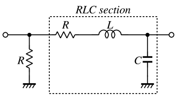
Fig. 1: Fundamental circuit structures

Fig. 2: Relative frequency response errors of reduced-order models for index-1 example obtained by (a)SPRBT-1 and (b)SPRBT-2

Fig. 3: Relative frequency response errors of reduced-order models for index-2 example obtained by (a)SPRBT-1 and (b)SPRBT-2

We calculated $30$ eigenvalues of the inverse Hamiltonian matrix ${\cal H}^{-1}$ for SPRBT-1 and ${\cal H}^{-1}{\cal E}$ for SPRBT-2 to obtain the shifts of RADI. Note that where reciprocal values were used, we use the label ”sml.” For comparison, $30$ eigenvalues of the Hamiltonian matrix ${\cal H}$ were also calculated using the Arnoldi method for SPRBT-1, in which the obtained values correspond to the large eigenvalues of the Hamiltonian matrix ${\cal H}$. For SPRBT-2, the shifts were calculated as follows [25]. Here, the generalized eigenvalue problem is expressed as ${\cal E}x=(1/\lambda){\cal H}x=t{\cal H}x$. Assuming an expansion point at $s=s_{0}$, the problem can be rewritten as $({\cal E}-s_{0}{\cal H})x=(t-s_{0}){\cal H}x$. The matrix pencil $s{\cal E}-{\cal H}$ is regular; thus, ${\cal E}-s_{0}{\cal H}$ is nonsingular. Therefore, the problem is described by $({\cal E}-s_{0}{\cal H})^{-1}{\cal H}x=1/(t-s_{0})x=\xi x$. Using the Arnoldi method, we obtain the approximate eigenvalues as $\lambda=1/(1/\xi+s_{0})$. Using the Krylov subspace method, large eigenvalues $\xi$ of matrix $({\cal E}-s_{0}{\cal H})^{-1}{\cal H}$ are obtained; thus, $\lambda$ also corresponds to a large generalized eigenvalue of $({\cal E},{\cal H})$. As $t$ should be small, $s_{0}$ is assumed to be a small negative value. Note that where these shifts were used, we use the label ”lrg.”

Figures 2(a) and 2(b) shows the frequency response errors obtained by SPRBT-1 and SPRBT-2, respectively, for the index-1 example, in which 30 RADI steps with 15 shifts were applied and $15$ order models were generated. The responses of sml are satisfactory for both SPRBT-1 and SPRBT-2, which implies that the suitable shifts were obtained. The responses of lrg with $s_{0}=-10^{-5}$ are inaccurate at low frequencies; however, they are accurate at high frequencies, which implies that large eigenvalues contribute to model accuracy at high frequencies. Figures 3(a) and 3(b) show the frequency response errors obtained by SPRBT-1 and SPRBT-2, respectively, for the index-2 example, in which 30 RADI steps with 15 shifts were applied and $15$ order models were generated. Here, the responses of sml are accurate at low frequencies, which implies that shift selection with Algorithm 4 is also suitable for index-2 descriptor systems.

Table 1: Computational time and memory usage of SPRBT-1 with (a) RARI and (b) QADI for index-1 example

size	ADI [s]	Else [s]	Total [s]	memory [MB]
$3,001$	$0.11$	$0.68$	$0.79$	$1.50\times 10^{0}$
$300,001$	$12.25$	$36.44$	$48.69$	$1.50\times 10^{2}$
$30,000,001$	$1,289.85$	$3,657.96$	$4,947.81$	$1.50\times 10^{4}$

size	ADI [s]	Else [s]	Total [s]	memory [MB]
$3,001$	$0.51$	$0.57$	$1.08$	$1.50\times 10^{0}$
$300,001$	$48.41$	$36.54$	$84.95$	$1.50\times 10^{2}$
$30,000,001$	$5,399.45$	$3,629.05$	$9,028.50$	$1.50\times 10^{4}$

Table 2: Computational time and memory usage of SPRBT-2 with (a) RARI and (b) QADI for index-1 example

size	ADI [s]	Else [s]	Total [s]	memory [MB]
$3,001$	$0.11$	$0.62$	$0.73$	$1.60\times 10^{0}$
$300,001$	$11.66$	$39.08$	$50.74$	$1.60\times 10^{2}$
$30,000,001$	$1,202.00$	$3,721.13$	$4,923.13$	$1.59\times 10^{4}$

size	ADI [s]	Else [s]	Total [s]	memory [MB]
$3,001$	$0.66$	$0.62$	$1.28$	$1.60\times 10^{0}$
$300,001$	$71.81$	$40.50$	$112.31$	$1.60\times 10^{2}$
$30,000,001$	$7,838.62$	$3,889.46$	$11,728.07$	$1.59\times 10^{4}$

Table 3: Computational time and memory usage of SPRBT-1 with (a) RARI and (b) QADI for index-2 example

size	ADI [s]	Else [s]	Total [s]	memory [MB]
$3,001$	$0.12$	$0.46$	$0.57$	$2.74\times 10^{0}$
$300,001$	$14.09$	$34.73$	$48.82$	$2.74\times 10^{2}$
$30,000,001$	$2,326.66$	$5,134.52$	$7,461.18$	$2.74\times 10^{4}$

size	ADI [s]	Else [s]	Total [s]	memory [MB]
$3,001$	$0.63$	$0.51$	$1.14$	$2.70\times 10^{0}$
$300,001$	$59.13$	$34.72$	$93.85$	$2.74\times 10^{2}$
$30,000,001$	$18,073.48$	$4,984.57$	$23,058.05$	$2.74\times 10^{4}$

Table 4: Computational time and memory usage of SPRBT-2 with (a) RARI and (b) QADI for index-2 example

size	ADI [s]	Else [s]	Total [s]	memory [MB]
$3,001$	$0.16$	$0.79$	$0.95$	$2.55\times 10^{0}$
$300,001$	$18.39$	$62.71$	$81.11$	$2.54\times 10^{2}$
$30,000,001$	$3,005.42$	$7,608.21$	$10,613.63$	$2.54\times 10^{4}$

size	ADI [s]	Else [s]	Total [s]	memory [MB]
$3,001$	$0.73$	$0.83$	$1.56$	$2.55\times 10^{0}$
$300,001$	$76.73$	$60.06$	$136.79$	$2.54\times 10^{2}$
$30,000,001$	$19,702.38$	$7,3497.40$	$27,051.78$	$2.54\times 10^{4}$

6.4 Computational Time and Memory Usage

For the index-1 and index-2 examples, we measured the computational time and memory usage when applying RPRBT-1 and RPRBT-2. The simulations were performed on a computer with a 3.7-GHz Intel Xeon E5-1620 CPU and 32 GB of memory. In Tables 1-4, ”size” is the order of the descriptor system (1), ”ADI” is the computational time of RADI or QADI, ”Else” is the time except for RADI or QADI, ”Total” is the total calculation time, and ”Mem” is memory usage.

RPRBT-1 and RPRBT-2 were applied to the index-1 example, in which 20 RADI steps with 10 shifts were applied and 15 order models were generated. Tables 1 and 2 show the computational time and memory usage for RPRBT-1 and RPRBT-2, respectively, in which RADI is compared to QADI. As shown in Table 1, RADI is 4.2 times faster than QADI, and the total time using RADI is 1.8 times less than when using QADI. As shown in Table 2, RADI is 6.52 times faster than QADI, and the total time using RADI is 2.4 times less than when using QADI.

RPRBT-1 and RPRBT-2 were also applied to the index-2 example, in which 20 RADI steps with 10 shifts were applied and 15 order models were generated. Tables 3 and 4 show the computational time and memory usage for RPRBT-1 and RPRBT-2, respectively. As shown in Table 3, RADI is 7.7 times faster than QADI, and the total time using RADI is 3.1 times less than when using QADI. As shown in Table 4, RADI is 6.5 times faster than QADI, and the total time using RADI is 2.6 times less than when using QADI.

For the index-1 example, RPRBT-1 is nearly identical to RPRBT-2 relative to efficiency and memory usage when RADI was used. On the other hand, for the index-2 example, RPRBT-1 is 1.4 times faster than RPRBT-2 when RADI was used, and the memory usage of RPRBT-1 is compatible with that of RPRBT-2.

Consequently, solving AREs or GAREs is no longer dominant in the computational cost of PRBT. Moreover, the efficiency and memory usage of RPRBT-1 are nearly compatible to RPRBT-2 when RADI was used.

7 Conclusions

In this paper, we have presented reciprocal and PRBTs for index-1 and index-2 descriptor systems, for which two approaches based on AREs or GAREs have been proposed. Furthermore, RADI was introduced to solve AREs and GAREs. We have demonstrated that solving the Riccati equation is no longer dominant in the computational cost of PRBT. By comparing the two approaches, we have also shown that both methods are compatible relative to computational time and memory usage. In addition, some properties of ARE- and GARE-associated descriptor systems for passive electrical circuits have been provided.

Appendix A

Here, we prove Theorem 2. From the symmetry of $A_{0}$, $A_{11}=A_{11}^{T}$, $A_{22}=A_{22}^{T}$, and $A_{21}=A_{12}^{T}$, we can obtain $\hat{A}_{0}=I^{\prime}_{r}A_{s}$, where $A_{s}$ is a symmetric matrix. From (14), we can obtain $\hat{B}_{0}=I^{\prime}_{r}\hat{C}_{0}^{T}$ for an impedance matrix and $\hat{B}_{0}=-I^{\prime}_{r}\hat{C}_{0}^{T}$ for an admittance matrix. Then, the AREs (15) and (16) are rewritten respectively as follows:

$$\left(I^{\prime}_{r}A_{s}\mp I^{\prime}_{r}C_{0}^{T}DD^{T}C_{0}\right)^{T}X+X\left(I^{\prime}_{r}A_{s}\mp I^{\prime}_{r}C_{0}^{T}DD^{T}C_{0}\right)$$

$$+XI^{\prime}_{r}C_{0}^{T}DD^{T}C_{0}I^{\prime}_{r}X+C_{0}^{T}DD^{T}C_{0}=0,$$ (72)

$$\left(I^{\prime}_{r}A_{s}\mp I^{\prime}_{r}C_{0}^{T}DD^{T}C_{0}\right)^{T}I^{\prime}_{r}YI^{\prime}_{r}+I^{\prime}_{r}YI^{\prime}_{r}\left(I^{\prime}_{r}A_{s}\mp I^{\prime}_{r}C_{0}^{T}DD^{T}C_{0}\right)$$

$$+I^{\prime}_{r}YI^{\prime}_{r}I^{\prime}_{r}C_{0}^{T}DD^{T}C_{0}I^{\prime}_{r}I^{\prime}_{r}YI^{\prime}_{r}+C_{0}^{T}DD^{T}C_{0}=0,$$ (73)

where the minus and plus signs correspond to the impedance and admittance matrices, respectively. From (72) and (73), $X=I^{\prime}_{r}YI^{\prime}_{r}$, which indicates that $Y=I^{\prime}_{r}XI^{\prime}_{r}$.

For a hybrid matrix, we have $\hat{B}_{0}=I^{\prime}_{r}\hat{C}_{0}^{T}I^{\circ}_{m}$ from (7) and (14). As $\hat{D}_{0}=-I^{\circ}_{m}\hat{B}_{2}^{T}A_{22}^{-1}\hat{B}_{2}$, $DD^{T}=(\hat{D}_{0}+\hat{D}_{0}^{T})^{-1}$ becomes a block diagonal matrix; thus, the relationship $I^{\circ}_{m}DD^{T}I^{\circ}_{m}=DD^{T}$ is obtained. Using this relationship, the dual AREs are expressed as follows:

$$\left(I^{\prime}_{r}A_{s}-I^{\prime}_{r}C_{0}^{T}I^{\circ}_{m}DD^{T}C_{0}\right)^{T}X+X\left(I^{\prime}_{r}A_{s}-I^{\prime}_{r}C_{0}^{T}I^{\circ}_{m}DD^{T}C_{0}\right)$$

$$+XI^{\prime}_{r}C_{0}^{T}DD^{T}C_{0}I^{\prime}_{r}X+C_{0}^{T}DD^{T}C_{0}=0,$$ (74)

$$\left(I^{\prime}_{r}A_{s}-I^{\prime}_{r}C_{0}^{T}I^{\circ}_{m}DD^{T}C_{0}\right)^{T}I^{\prime}_{r}YI^{\prime}_{r}+I^{\prime}_{r}YI^{\prime}_{r}\left(I^{\prime}_{r}A_{s}-I^{\prime}_{r}C_{0}^{T}I^{\circ}_{m}DD^{T}C_{0}\right)$$

$$+I^{\prime}_{r}YI^{\prime}_{r}I^{\prime}_{r}C_{0}^{T}DD^{T}C_{0}I^{\prime}_{r}I^{\prime}_{r}XI^{\prime}_{r}+C_{0}^{T}DD^{T}C_{0}=0.$$ (75)

From (74) and (75), we obtain $X=I^{\prime}_{r}YI^{\prime}_{r}$, which indicates that $Y=I^{\prime}_{r}XI^{\prime}_{r}$.

Appendix B

Here, we prove the equations in (36). Using (9), we obtain the following relation:

$$-\bar{C}_{0}\left(I_{n}-P_{r}\right)\bar{A}_{0}^{-1}\left(I_{n}-P_{l}\right)\bar{B}_{0}$$

$$= -\bar{C}_{0}T_{r}^{-1}\left[\begin{array}[]{cc}0&0\\ 0&I_{n-r}\end{array}\right]\left[\begin{array}[]{cc}J^{-1}&0\\ 0&I_{n-r}\end{array}\right]\left[\begin{array}[]{cc}0&0\\ 0&I_{n-r}\end{array}\right]T_{l}^{-1}\bar{B}_{0}$$

$$= -C_{\infty}B_{\infty}.$$

Then, $M_{0}$ is obtained by adding $\bar{D}_{0}$ to it. Similarly, $M_{1}$ of (36) is given as follows:

$$-\bar{C}_{0}\bar{A}_{0}^{-1}\left(I_{n}-P_{l}\right)\bar{E}_{0}\left(I_{n}-P_{r}\right)\bar{A}_{0}^{-1}\bar{B}_{0}$$

$$= -\bar{C}_{0}T_{r}^{-1}\left[\begin{array}[]{cc}J^{-1}&0\\ 0&I_{n-r}\end{array}\right]\left[\begin{array}[]{cc}0&0\\ 0&I_{n-r}\end{array}\right]$$

$$\times\left[\begin{array}[]{cc}I_{r}&0\\ 0&N\end{array}\right]\left[\begin{array}[]{cc}0&0\\ 0&I_{n-r}\end{array}\right]\left[\begin{array}[]{cc}J^{-1}&0\\ 0&I_{n-r}\end{array}\right]T_{l}^{-1}\bar{B}_{0}$$

$$= -C_{\infty}NB_{\infty}.$$

Appendix C

Here, we prove Theorem 4 with the dual projected generalized Lur’e equations rather than dual GAREs (37) and (38). The dual GAREs (37) and (38) are respectively equivalent to the projected generalized Lur’e equations:

$$\left\{\begin{aligned} \bar{A}_{0}^{T}X\bar{E}_{0}+\bar{E}_{0}^{T}X\bar{A}_{0}&=-K_{o}^{T}K_{o},\quad X=P_{l}^{T}XP_{l}\\ \bar{E}_{0}^{T}X\bar{B}_{0}-P_{r}^{T}\bar{C}_{0}^{T}&=-K_{o}^{T}J_{o},\quad M_{o}+M_{o}^{T}=J_{o}^{T}J_{o}\end{aligned}\right.$$ (79)

$$\left\{\begin{aligned} \bar{A}_{0}Y\bar{E}_{0}^{T}+\bar{E}_{0}Y\bar{A}_{0}^{T}&=-K_{c}K_{c}^{T},\quad Y=P_{r}YP_{r}^{T}\\ \bar{E}_{0}Y\bar{C}_{0}^{T}-P_{l}\bar{B}_{0}&=-K_{c}J_{c}^{T},\quad M_{o}+M_{o}^{T}=J_{c}J_{c}^{T}\end{aligned}\right.$$ (80)

For an impedance matrix, $\bar{E}_{0}=\bar{E}_{0}^{T}$, $\bar{A}_{0}=\bar{A}_{0}^{T}$, and $\bar{B}_{0}=\bar{C}_{0}^{T}$ hold. Using the relationship $P_{l}=P_{r}^{T}$ and rewriting $K_{c}$ and $J_{c}$ with $K_{o}^{T}$ and $J_{o}^{T}$ in (80), respectively, we confirm that $X=Y$. Similar to the impedance matrix case, $X=Y$ for an admittance matrix.

For a hybrid matrix, $\bar{E}_{0}=\bar{E}_{0}^{T}$, $\bar{A}_{0}=\bar{A}_{0}^{T}$, and $\bar{B}_{0}=\bar{C}_{0}^{T}I^{\circ}_{m}$ hold. Using the relationship $P_{l}=P_{r}^{T}$, we can write the third equation of (79) as $\bar{E}_{0}X\bar{C}_{0}^{T}I^{\circ}_{m}-P_{l}\bar{B}_{0}I^{\circ}_{m}=-K^{T}_{o}J_{o}$. Here, $M_{0}$ is block skew symmetric; thus, $J_{o}^{T}J_{o}=I^{\circ}_{m}J_{o}^{T}J_{o}I^{\circ}_{m}$. This implies that $J_{o}=J_{o}I^{\circ}_{m}$. Therefore, the dual Lur’e equations are identical and $X=Y$ for the hybrid matrix.

References

• [1] O. Abidi, M. Hached, and K. Jbilou, “Adaptive rational block Arnoldi methods for model reductions in large-scale MIMO systems,” New Trends in Mathematical Sciences, 4 (2016), pp. 227-239.
• [2] L. Amodei and J.-M. Buchot, “An invariant subspace method for lage-scale algebraic Riccati equation,”, Appl. Numer. Math., 60 (2010), pp. 1067-1082.
• [3] B. D. Anderson and S. Vongpanitlerd, Network Analysis and Synthesis, Englewood Cliffs, NJ: Prentice-Hall, 1973.
• [4] G. Ali, N. Banagaaya, W. H. A. Schilders, and C. Tischendorf, “Index-aware model order reduction for index-2 differential-algebraic equations,,” SIAM J. Sci. Comput., 35 (2013), pp. 1487-1510.
• [5] P. Benner, Z. Bujanović, P. Kürschner, J. Saak, “RADI: A low-rank ADI-type algorithm for large scale algebraic Riccati equations,” Numerische Mathematik, (2017), DOI 10.1007/s00211-017-0907-5.
• [6] P. Benner and T. Stykel, “Numerical solution of projected algebraic Riccati equations,” SIAM J. Numer. Anal., 52 (2014), pp. 581–600.
• [7] P. Benner and Z. Bujanović, “On the solution of large-scale algebraic Riccati equations by using low-dimensional invariant subspaces,” Linear Algebra and its Applications, 488 (2016), pp. 430-459.
• [8] V. Druskin and V. Simoncini, “Adaptive rational Krylov subspaces for large-scale dynamical systems,” Systems Control Lett., 60 (2011), pp. 546-560.
• [9] V. Druskin, L. Knizhnerman, V. Simoncini, “Analysis of the rational Krylov subspace and ADI methods for solving the Lyapunov equation,” SIAM. J. Numer. Anal., 49 (2011), pp. 1875-1898.
• [10] P. Feldmann and R. W. Freund, “Efficient linear analysis by Padé approximation via the Lanczos process,” IEEE Trans. Computer-Aided Design Integr. Circuit Syst., 14 (1995), pp. 639-649.
• [11] G. H. Goulb and C. F. Van Loan, Matrix Computation, The Johns Hopkins University Press, 2012.
• [12] S. Gugercin, T. Stykel, and S. Wyatt, “Model reduction of descriptor systems by interpolatory projection methods,” SIAM J. Sci. Comput., 35 (2013), pp. B1010-B1033.
• [13] E. J. Grimme, ”Krylov projection methods for model reduction,” Ph.D. dissertation, University of Illinois at Urbana-Champaign, 1997.
• [14] M. Heinkenschloss, D. C. Sorensen, and K. Sun, “Balanced truncation model reduction for a class of descriptor systems with application to the oseen equations,” SIAM J. Sci. Comput., 30 (2008), pp. 1038-1063.
• [15] M. Heyouni and K. Jbilou, ”An extended block Arnoldi algorithm for large-scale solutions of the continuous-time algebraic Riccati equation,” Electron. Trans. Numer. Anal., 33 (2009), pp. 53-62.
• [16] K. Jbilou, “Block Krylov subspace methods for large algebraic Riccati equations,” Numer. Algorithms, 34 (2003), pp. 339-353.
• [17] T. Katayama, Senkei-System-no-Saiteki-Seigyo, Kindai Kagaku Sya (in Japanese).
• [18] Y. Lin and V. Simoncini, “A new subspace iteration method for the algebraic Riccati equation,” Numerical Linear Algebra with Application, 22 (2015), pp. 26-47.
• [19] A. Massoudi, M. Opmeer, and T. Reis, “The ADI method for bounded real and positive real Lur’e equations,” Numerische Mathematik, 135 (2017), pp. 431–458.
• [20] B. Moore, “Principal component analysis in linear systems: Controllability, observability, and model reduction,” IEEE Trans. Automat. Contr., 26 (1981), pp. 17-32.
• [21] A. Odabasioglu, M. Celik, and L. T. Pileggi, “PRIMA: passive reduced-order interconnect macromodeling algorithm,” IEEE Trans. Computer-Aided Design Integr. Circuit Syst., 17 (1998), pp. 645-654.
• [22] J. R. Phillips, L. Daniel, and L. M. Silveira, “Guaranteed passive balancing transformations for model order reduction,” IEEE Trans. Computer-Aided Design Integr. Circuit Syst., 22 (2003), pp. 1-15.
• [23] T. Reis and T. Stykel, “Positive real and bounded real balancing for model reduction of descriptor systems,” Int. J. Control, 83 (2008), pp. 74–88.
• [24] T. Reis and T. Stykel “PABTEC: Passivity-preserving balanced truncation for electrical circuits,” IEEE Trans. Computer-Aided Design Integr. Circuit Syst., 29 (2010), pp. 1354-1367.
• [25] Y. Tanji, “Low-rank solutions of Riccati equations for positive real balanced truncations of RLC networks,” Nonlinear Theory and Its Applications, IEICE, 9 (2018), pp. 479-496.
• [26] N. Wong and V. Balakrishnan, “Fast positive-real balanced truncation via quadratic alternating direction implicit iteration,” IEEE Trans. Computer-Aided Design Integr. Circuit Syst., 26 (2007), pp. 1725-1731.
• [27] Z. Zhang and N. Wong, “An efficient projector-based passivity test for descriptor systems, IEEE Trans. Comput. -Aided Design Integr. Circuit Syst., 29 (2010), pp. 1203–1214.
• [28] K. Zhou, J. C. Doyle, and K. Glover, Robust and Optimal Control, NJ: Prentice Hall, 1995.