Time-changed Poisson processes of order $k$

Abstract.

In this article, we study the Poisson process of order $k$ (PPoK) time-changed with an independent Lévy subordinator and its inverse, which we call respectively, as TCPPoK-I and TCPPoK-II, through various distributional properties, long-range dependence and limit theorems for the PPoK and the TCPPoK-I. Further, we study the governing difference-differential equations of the TCPPoK-I for the case inverse Gaussian subordinator. Similarly, we study the distributional properties, asymptotic moments and the governing difference-differential equation of TCPPoK-II. As an application to ruin theory, we give a governing differential equation of ruin probability in insurance ruin using these processes. Finally, we present some simulated sample paths of both the processes.

1. Introduction

Poisson process can be considered as a core object of applied probability, due to its simplicity and applicability in modelling count data, which led to evolution and generalization of Poisson processes in several directions. For example, non-homogeneous Poisson processes, Cox point processes, higher dimensional Poisson processes, and for last two decades, the fractional (time-changed) variants of Poisson processes (see [22, 28, 7, 31] and references therein) have caught the attention of the researchers and a vast literature is available on this topic. In particular, insurance models generally use Poisson process to model the arrival of claims with a limitation of not having more than one claim in a certain small time interval. However, the claim arrival in group insurance schemes may contain more than one claims. To overcome this difficulty, Kostadinova and Minkova (2012) [19] introduced a variant known as Poisson process of order $k$, which models the claim arrival in groups of size $k$, where the number of arrivals in a group is uniformly distributed over $k$ points. Further, in case of calamities, the time period between two claims may not have exponential distribution, as these are extreme events and can not be modelled by Poisson process of order $k$ (as defined in [19]). Hence there is a need to generate a new stochastic process which is a generalization of Poisson process of order $k$. Among various techniques to create a new process, the technique of subordination (or time-change) introduced by Bohner [9] has gained significant attention in recent years. The theory of subordinated processes is explored in detail in [35]. A subordinated stochatic process can be generated by replacing time of the original process with a stochastic process preferably having non-decreasing sample paths. In literature, various examples of subordinated processes are discussed, and shown to have interesting probabilistic properties and elegant connections to fractional calculus, see e.g. [1, 2, 4, 7, 18, 36]. In paricular, recently, subordinated Poisson processes are studied by several authors (see [20, 31, 42, 23, 24, 32]). Also, these processes are extensively used in several areas, such as physics [29, 16, 39, 15, 5, 6], ecology [37], biology [17], hydrology [27] and finance [12, 26, 14, 11, 25]. However, to the best of our knowledge, subordinated Poisson processes of order $k$ have not been explored. In this article, the main goal is to explore time-changed Poisson process of order $k$ with Lévy subordinator (increasing Lévy process) and its right-continuous inverse, as the transition probabilities of the new process with Lévy subordinator allow us to have more than one arrivals in a small interval of time which is useful in modelling the count data occurring in lumps.

The article is organized as follows. Section 2 deals with some preliminary definitions and results. In Sections 3 and 4, Poisson process of order $k$ with a Lévy subordinator and its right-continuous inverse are studied, respectively. The governing equations for the time-changed Poisson process of order $k$ are given in Section 5. Section 6 discusses an application in ruin theory. Finally, some simulation algorithms to generate the sample paths of these processes are presented in Section 7.

2. Preliminaries

In this section, we state some relevant definitions and results related to Poisson process of order $k$ and Lévy subordinator.

2.1. Poisson distribution of order $k$

The early work on the distributions of order $k$ started with defining the notion geometric distribution of order $k$ (see [34]) which denotes the number of trials until the first occurrence of $k$ consecutive successes in a sequence of independent Bernoulli trials. The probability distribution of the sum of independent and identically distributed (IID) random variables having geometric distribution of order $k$ is called negative binomial distribution of order $k$ (NBoK). Let $Y_{n}$ denote NBoK, then the limiting distribution of $\{Y_{n}-kn\}$ as $n\to\infty$ is termed as Poisson distribution of order $k$ (PoK) (see [34, Theorem 3.2]).

Definition 1.

Let $x_{1},x_{2},\ldots,x_{k}$ be non-negative integers and $\zeta_{k}=x_{1}+x_{2}+\ldots+x_{k}$, $\Pi_{k}!=x_{1}!x_{2}!\ldots x_{k}!$ and

(1) $$\Omega(k,n):=\left\{{\bf x}=(x_{1},x_{2},\ldots,x_{k})\big{|}x_{1}+2x_{2}+\ldots+kx_{k}=n\right\}.$$

Also, let $N^{(k)}$ follow PoK with rate parameter $\lambda>0$, then the probability mass function (pmf) is given by

$$\mathbb{P}[N^{(k)}=n]=\sum_{{\bf x}\in\Omega(k,n)}e^{-k\lambda}\frac{\lambda^{\zeta_{k}}}{\Pi_{k}!},\leavevmode\nobreak\ n=0,1,\ldots.$$

The probability generating function (pgf) is given by (see [33, Lemma 2.2])

(2) $$G_{N^{(k)}}(s)=e^{-\lambda\left(k-\sum_{i=1}^{k}s^{i}\right)}.$$

It is also known that (see [19]) the PoK has the following compound Poisson representation

(3) $$N^{(k)}\stackrel{{\scriptstyle d}}{{=}}\sum_{i=0}^{N}X_{i},$$

where $N$ is Poisson random variable with rate parameter $k\lambda>0$, $X_{0}\equiv 0$, and $\{X_{i}\}_{i\geq 1}$is a sequence of IID discrete uniform random variable with pmf given by $\mathbb{P}[X_{i}=j]=1/k,\leavevmode\nobreak\ j=1,2,\ldots,k$, which is independent of $N$. Then the pgf of $X_{1}$ is given by $G_{X_{1}}(s)=\frac{s}{k}\frac{1-s^{k}}{1-s}$, $s\in(0,1).$ Therefore, the pgf of $N^{(k)}$ given in (3) is

(4) $$G_{N^{(k)}}(s)=G_{N}(G_{X_{1}}(s))=e^{-k\lambda(1-G_{X_{1}}(s))}.$$

It can be easily seen that pgf obtained in (2) and (4) are same.

2.2. The Poisson process of order $k$

The Poisson process of order $k$ (PPoK) is introduced and studied by Kostadinova and Minkova (see [19]) which can be defined as follows.

Definition 2.

Let $\{N(t,k\lambda)\}_{t\geq 0}$ denote Poisson process with rate parameter $k\lambda>0$, $X_{0}\equiv 0$, and $\{X_{i}\}_{i\geq 1}$ be a sequence of IID discrete uniform random variables over $k$ points. Then the PPoK, $\{N^{(k)}(t,\lambda)\}_{t\geq 0}$, is defined (see [19]) as

$$N^{(k)}(t,\lambda)=\sum_{i=0}^{N(t,k\lambda)}X_{i},$$

where $\{X_{i}\}_{i\geq 1}$ and $\{N(t,k\lambda)\}_{t\geq 0}$ are assumed to be independent.

Henceforth, for brevity, the parameter $\lambda$ is suppressed and $N^{(k)}(t,\lambda)$ is written as $N^{(k)}(t)$, when no confusion arises.

Remark 2.1.

For $k=1$, the distribution of $X_{i}$’$s$ degenerate to Dirac-delta distribution at 1 and $\{N^{(1)}(t)\}_{t\geq 0}$ reduces to the Poisson process $\{N(t)\}_{t\geq 0}$.

Remark 2.2.

The pgf of $N^{(k)}(t)$ is $G_{N^{(k)}(t)}(s)=\exp\left(-k\lambda t(1-G_{X_{1}}(s))\right)$, where $G_{X_{1}}(s)=\frac{s}{k}\frac{1-s^{k}}{1-s}$ is the pgf of $X_{1}$.

The mean, variance and covariance function of the PPoK are given by

$$\mathbb{E}[N^{(k)}(t)] =\frac{k(k+1)}{2}\lambda t$$

$$\mbox{Var}[N^{(k)}(t)] =\frac{k(k+1)(2k+1)}{6}\lambda t$$

$$\mbox{Cov}[N^{(k)}(s),N^{(k)}(t)] =\frac{k(k+1)(2k+1)}{6}\lambda\min(s,t).$$

Also, observe that the transition probabilities of the PPoK $\{N^{(k)}(t)\}_{t\geq 0}$ are given by

$$\mathbb{P}[N^{(k)}(t+h)=n|N^{(k)}(t)=m]=\left\{\begin{array}[]{ll}1-k\lambda h+o(h)&\mbox{if }n=m,\\ \lambda h+o(h)&\mbox{if }n=m+i,i=1,2,\ldots,k.\end{array}\right.$$

Let $p_{m}(t)=\mathbb{P}[N^{(k)}(t)=m],m=0,1,2,\ldots$ denote the pmf of PPoK, then

$$\frac{d}{dt}p_{0}(t) =-k\lambda p_{0}(t),$$

(5) $$\frac{d}{dt}p_{m}(t) =-k\lambda p_{m}(t)+\lambda\sum_{j=1}^{m\wedge k}p_{m-j}(t),\leavevmode\nobreak\ m=1,2,\ldots,$$

with initial condition $p_{0}(0)=1\text{ and }p_{m}(0)=0,m=1,2,\ldots$ and $m\wedge k:=\min\{m,k\}.$

Next, note that the pgf of $\{N^{(k)}(t)\}_{t\geq 0}$ satisfies the following differential equation

$$\frac{\partial}{\partial t}G_{N^{(k)}(t)}(s)=-k\lambda[1-G_{X_{1}}(s)]G_{N^{(k)}(t)}(s),\leavevmode\nobreak\ \leavevmode\nobreak\ {\rm with}\leavevmode\nobreak\ \leavevmode\nobreak\ G_{N^{(k)}(0)}(0)=1.$$

The Lévy exponent (characteristic exponent) (see [13]) of $\{N^{(k)}(t)\}_{t\geq 0}$ is given by

$$\psi(u)=\int_{-\infty}^{\infty}k\lambda(\exp(\iota uy)-1)\mu_{X_{1}}(dy).$$

2.3. Lévy subordinator

A Lévy subordinator (hereafter referred to as the subordinator) $\{D_{f}(t)\}_{t\geq 0}$ is a non-decreasing Lévy process and its Laplace transform (LT) (see [3, Section 1.3.2]) has the form

(6) $$\mathbb{E}[e^{-sD_{f}(t)}]=e^{-tf(s)},\;{\rm where}\;f(s)=bs+\int_{0}^{\infty}(1-e^{-sx})\nu(dx),\leavevmode\nobreak\ b\geq 0,s>0,$$

is the Bernstein function (see [38] for more details). Here $b$ is the drift coefficient and $\nu$ is a non-negative Lévy measure on positive half-line satisfying

$$\int_{0}^{\infty}(x\wedge 1)\nu(dx)<\infty\leavevmode\nobreak\ \leavevmode\nobreak\ {\rm and}\leavevmode\nobreak\ \leavevmode\nobreak\ \nu([0,\infty))=\infty$$

which ensures that the sample paths of $D_{f}(t)$ are almost surely $(a.s.)$ strictly increasing. Also, the first-exit time of $\{D_{f}(t)\}_{t\geq 0}$ is defined as $E_{f}(t)=\inf\{r\geq 0:D_{f}(r)>t\}$,which is the right-continuous inverse of the subordinator $\{D_{f}(t)\}_{t\geq 0}$.

Remark 2.3.

Note that a Lévy subordinator is a class of subrodinators, which is useful in generating various subordinated stochastic processes in general. Next, we include some well-known examples of Lévy subordinators with drift coefficient $b=0$ which are used later in the article.

1. Let the Lévy measure be $\nu(dx)=\frac{pe^{-\alpha x}}{x}dx,\leavevmode\nobreak\ x>0,p>0,\alpha>0$ then using (6), we get the Gamma subordinator $\{Y(t)\}_{t\geq 0}$ with Bernstein function $f(s)=p\log(1+\frac{s}{\alpha})$ (see [13], p. 115).

2. Let the Lévy measure be $\nu(dx)=c\frac{e^{-\mu x}}{x^{\alpha+1}}dx,\leavevmode\nobreak\ x>0,c>0,\mu>0,0<\alpha<1$ then using (6), we get the Tempered $\alpha$-stable subordinator $D_{\alpha}^{\mu}(t)$ with Bernstein function $f(s)=(s+\mu)^{\alpha}-\mu^{\alpha}$ (see [13], p. 115).

3. Let the Lévy measure be $\nu(dx)=\frac{\delta}{\sqrt{2\pi x^{3}}}e^{\frac{-\gamma^{2}x}{2}}dx,\leavevmode\nobreak\ x>0,\gamma>0,\delta>0$ then using (6), we get the Inverse Gaussian subordinator $G(t)$ with Bernstein function $f(s)=\delta(\sqrt{2s+\gamma^{2}}-\gamma)$ (see [41]).

3. Time-changed Poisson process of order $k$ - I

In this section, we consider the PPoK with a subordinator $\{D_{f}(t)\}_{t\geq 0}$, satisfying $\mathbb{E}[D_{f}^{\rho}(t)]<\infty$ for all $\rho>0$, which can be defined as follows.

Definition 3.

The time-changed PPoK of Type-I (TCPPoK-I) is defined as

$$\{Q_{f}^{(1)}(t)\}=\{N^{(k)}(D_{f}(t))\},\leavevmode\nobreak\ \leavevmode\nobreak\ t\geq 0$$

where $\{N^{(k)}(t)\}_{t\geq 0}$ is the PPoK and is independent of the subordinator $\{D_{f}(t)\}_{t\geq 0}$.

Next, we derive some properties of the TCPPoK-I. Let us first compute its pmf.

Theorem 3.1.

Let the Bernstein function $f(s)$, as defined in (6), be such that $\mathbb{E}[D_{f}^{\rho}(t)]<\infty$ for all $\rho>0$. Then, the pmf of the TCPPoK-I is given by

(7) $$P[Q_{f}^{(1)}(t)=n]=\sum_{{\bf x}\in\Omega(k,n)}\frac{\lambda^{\zeta_{k}}}{\Pi_{k}!}\mathbb{E}\left[e^{-k\lambda D_{f}(t)}D_{f}^{\zeta_{k}}(t)\right],\leavevmode\nobreak\ \leavevmode\nobreak\ n=0,1,2,\ldots.$$

Proof.

Let $g_{f}(y,t)$ be the probability density function (pdf) of Lévy subordinator. Then

$$P[Q_{f}^{(1)}(t)=n]=P[N^{(k)}(D_{f}(t))=n]= \int_{0}^{\infty}P[N^{(k)}(D_{f}(t))=n|D_{f}(t)]g_{f}(y,t)dy$$

$$= \int_{0}^{\infty}\sum_{{\bf x}\in\Omega(k,n)}\frac{e^{-k\lambda y}(\lambda y)^{\zeta_{k}}}{\Pi_{k}!}g_{f}(y,t)dy$$

$$= \sum_{{\bf x}\in\Omega(k,n)}\frac{\lambda^{\zeta_{k}}}{\Pi_{k}!}\mathbb{E}\left[e^{-k\lambda D_{f}(t)}D_{f}^{\zeta_{k}}(t)\right],$$

which completes the proof. ∎

Corollary 3.1.

The pmf of the TCPPoK-I satisfies the normalizing condition

$$\sum_{n=0}^{\infty}P[Q_{f}^{(1)}(t)=n]=1.$$

Proof.

We first prove this result for the case $k=2$. From (7) we have

$$\sum_{n=0}^{\infty}P[Q_{f}^{(1)}(t)=n]=\sum_{n=0}^{\infty}\sum_{{\bf x}\in\Omega(2,n)}\frac{\lambda^{\zeta_{2}}}{\Pi_{2}!}\mathbb{E}\left[e^{-2\lambda D_{f}(t)}D_{f}^{\zeta_{2}}(t)\right].$$

Set $x_{i}=n_{i}\leavevmode\nobreak\ i=1,2$ and $n=x+\sum_{i=1}^{2}(i-1)n_{i}$ in the above expression. Then

$$\sum_{n=0}^{\infty}P[Q_{f}^{(1)}(t)=n]= \sum_{x+n_{2}=0}^{\infty}\sum_{\begin{subarray}{c}n_{1},n_{2}\geq 0\\ n_{1}+n_{2}=x\end{subarray}}\frac{\lambda^{n_{1}+n_{2}}}{n_{1}!n_{2}!}\mathbb{E}\left[e^{-2\lambda D_{f}(t)}D_{f}^{n_{1}+n_{2}}(t)\right]$$

$$= \sum_{x=0}^{\infty}\frac{(2\lambda)^{x}}{x!}\mathbb{E}\left[e^{-2\lambda D_{f}(t)}D_{f}^{x}(t)\right]\text{(using binomial theorem)}$$

$$= \int_{0}^{\infty}e^{-2\lambda y}\sum_{x=0}^{\infty}\frac{(2\lambda)^{x}}{x!}y^{x}g_{f}(y,t)dy$$

$$= \int_{0}^{\infty}e^{-2\lambda y}e^{2\lambda y}g_{f}(y,t)dy=\int_{0}^{\infty}g_{f}(y,t)dy=1.$$

Using similar arguments one can prove for higher values of $k$. ∎

Using simple algebraic calculations, one can see that the transition probabilities of the TCPPoK-I $\{Q_{f}^{(1)}(t)\}_{t\geq 0}$ are given by

(8) $$\mathbb{P}[Q_{f}^{(1)}(t+h)=n|Q_{f}^{(1)}(t)=m]=\begin{cases}1-hf(k\lambda)+o(h),&n=m\\ &\\ -h\left(\sum\limits_{{\bf x}\in\Omega(k,i)}\frac{(-\lambda)^{\zeta_{k}}}{\Pi_{k}!}f^{(\zeta_{k})}(k\lambda)\right)+o(h),&n=m+i,\leavevmode\nobreak\ i=1,2,\ldots\end{cases},$$

where $f(k\lambda)$ is the Bernstein function.
Further, we present some interesting examples for the TCPPoK-I.

Example 3.1 (Negative Binomial process of order $k$).

It is known that negative binomial process can be obtained by subordinating the Poisson process with gamma process (see [42]). In a similar spirit, we can define the negative binomial process of order $k$ by subordinating PPoK with an independent gamma process $\{Y(t)\}_{t\geq 0}$ as defined in Remark 2.3(i) and its pmf is given by

$$\mathbb{P}[N^{(k)}(Y(t))=n]=\sum_{{\bf x}\in\Omega(k,n)}\frac{\lambda^{\zeta_{k}}}{\Pi_{k}!}\sum_{m=0}^{\infty}\frac{(-k\lambda)^{m}}{m!}\frac{\Gamma(pt+\zeta_{k}+m)}{\alpha^{\zeta_{k}+m}\Gamma(pt)},\leavevmode\nobreak\ n=0,1,2,\ldots.$$

Example 3.2 (Poisson-tempered $\alpha$-stable process of order $k$).

Let $\{D_{\alpha}^{\mu}(t)\}_{t\geq 0},\leavevmode\nobreak\ \mu>0,\leavevmode\nobreak\ 0<\alpha<1$ be the tempered $\alpha$-stable subordinator as defined in Remark 2.3(ii). Then pmf of the Poisson-tempered $\alpha$-stable of order $k$ is given by

$$\mathbb{P}[N(D_{\alpha}^{\mu}(t))=n]=\sum_{{\bf x}\in\Omega(k,n)}\frac{(\lambda)^{\zeta_{k}}}{\Pi_{k}!}e^{\mu^{\alpha}t}\sum_{m=0}^{\infty}\frac{(-k\lambda)^{m}}{m!}\mathbb{E}[(D_{\alpha}(t))^{\zeta_{k}+m}e^{-\mu D_{\alpha}(t)}],n=0,1,2,\ldots.$$

Example 3.3 (Poisson-inverse Gaussian process of order $k$).

Let $\{G(t)\}_{t\geq 0}$ be the inverse Gaussian subordinator as defined in Remark 2.3(iii). The moments of $\{G(t)\}_{t\geq 0}$ are given by (see [42])

$$\mathbb{E}[G^{q}(t)]=\sqrt{\frac{2}{\pi}}\delta\left(\frac{\delta t}{\gamma}\right)^{q-\frac{1}{2}}te^{\delta\gamma t}K_{q-\frac{1}{2}}(\delta\gamma t),\leavevmode\nobreak\ \leavevmode\nobreak\ \delta,\gamma>0,\leavevmode\nobreak\ t\geq 0,\leavevmode\nobreak\ q\in(-\infty,\infty),$$

where $K_{\nu}(z)$ is the modified Bessel function of third kind with index $\nu$, defined by

$$K_{\nu}(\omega)=\frac{1}{2}\int_{0}^{\infty}x^{\nu-1}e^{\frac{-1}{2}\omega(x+x^{-1})}dx,\leavevmode\nobreak\ \omega>0.$$

Using the above expression, we get the following

$$\mathbb{E}[G^{\zeta_{k}+m}(t)]=\sqrt{\frac{2}{\pi}}\delta\left(\frac{\delta t}{\gamma}\right)^{(\zeta_{k}+m)-\frac{1}{2}}te^{\delta\gamma t}K_{(\zeta_{k}+m)-\frac{1}{2}}(\delta\gamma t),$$

where $\delta,\gamma>0,\leavevmode\nobreak\ t\geq 0.$ Substituting above values of moments in Theorem 3.1, we get the pmf of Poisson-inverse Gaussian process of order $k$.

Next, we discuss some distributional properties of TCPPoK-I.

Theorem 3.2.

Let $0<s\leq t<\infty$, then the mean and covariance function of TCPPoK-I are as follows

1. $\mathbb{E}[Q_{f}^{(1)}(t)]=\frac{k(k+1)}{2}\lambda\mathbb{E}[D_{f}(t)],$

2. $\text{Cov}[Q_{f}^{(1)}(s),Q_{f}^{(1)}(t)]=\frac{k(k+1)(2k+1)}{6}\lambda\mathbb{E}[D_{f}(s)]+(\frac{k(k+1)}{2}\lambda)^{2}\text{Var}[D_{f}(s)],$

Proof.

Let $g_{f}(y,t)$ be the pdf of the Lévy subordinator $\{D_{f}(t)\}_{t\geq 0}$. Then

$$\mathbb{E}[Q_{f}^{(1)}(t)]=\mathbb{E}[N^{(k)}(D_{f}(t))]=\mathbb{E}[\mathbb{E}[N^{(k)}(D_{f}(t))|D_{f}(t)]]=\frac{k(k+1)}{2}\lambda\mathbb{E}[D_{f}(t)],$$

which proves Part (i).

Now, we derive the expression for covariance of TCPPoK-I. First, we evaluate $\mathbb{E}[Q_{f}^{(1)}(s)Q_{f}^{(1)}(t)]$.

$$\mathbb{E}[Q_{f}^{(1)}(s)Q_{f}^{(1)}(t)]= \mathbb{E}[N^{(k)}(D_{f}(s))N^{(k)}(D_{f}(t))]$$

$$= \mathbb{E}[N^{(k)}(D_{f}(s))\{N^{(k)}(D_{f}(t))-N^{(k)}(D_{f}(s))\}]+\mathbb{E}[(N^{(k)}(D_{f}(s)))^{2}]$$

$$= \mathbb{E}[N^{(k)}(D_{f}(s))]\mathbb{E}[N^{(k)}(D_{f}(t))-N^{(k)}(D_{f}(s))]+\mathbb{E}[(N^{(k)}(D_{f}(s)))^{2}]$$

$$= \mathbb{E}[N^{(k)}(D_{f}(s))]\mathbb{E}[N^{(k)}(D_{f}(t-s))]+\mathbb{E}[(N^{(k)}(D_{f}(s)))^{2}]$$

$$= \frac{k(k+1)}{2}\lambda\mathbb{E}[D_{f}(s)]\frac{k(k+1)}{2}\lambda\mathbb{E}[D_{f}(t-s)]+$$

$$\frac{k(k+1)(2k+1)}{6}\lambda\mathbb{E}[D_{f}(s)]+\left(\frac{k(k+1)\lambda}{2}\right)^{2}\mathbb{E}[(D_{f}(s))^{2}],$$

where the last equality follows from the fact that

$$\mathbb{E}[(N^{(k)}(D_{f}(s)))^{2}]=\frac{k(k+1)(2k+1)}{6}\lambda\mathbb{E}[D_{f}(s)]+\left(\frac{k(k+1)\lambda}{2}\right)^{2}\mathbb{E}[(D_{f}(s))^{2}].$$

Therefore, we get

$$Cov[Q_{f}^{(1)}(s),Q_{f}^{(1)}(t)]= \mathbb{E}[Q_{f}^{(1)}(s)Q_{f}^{(1)}(t)]-\mathbb{E}[Q_{f}^{(1)}(s)]\mathbb{E}[Q_{f}^{(1)}(t)]$$

$$= \frac{k(k+1)(2k+1)}{6}\lambda\mathbb{E}[D_{f}(s)]+\left(\frac{k(k+1)}{2}\lambda\right)^{2}\text{Var}[D_{f}(s)].$$

which completes the proof of Part (ii). To get the expression of variance of the TCPPoK-I, we can put $s=t$ in the Part (ii). ∎

Remark 3.1.

From Theorem 3.2, it is clear that $Var[Q_{f}^{(1)}(t)]>\mathbb{E}[Q_{f}^{(1)}(t)]$.Therefore, the index of dispersion $I(t):=Var[Q_{f}^{(1)}(t)]/\mathbb{E}[Q_{f}^{(1)}(t)]$ (see [24] for more details) is greater than 1. Hence, we conclude that TCPPoK-I exhibits overdispersion.

3.1. Long-range dependence

Now we discuss the long-range dependence (LRD) property of the TCPPoK-I. We first need the following definitions.

Definition 4.

Let $f(x)$ and $g(x)$ be positive functions. We say that $f(x)$ is asymptotically equal to $g(x)$, written as $f(x)\sim g(x),\leavevmode\nobreak\ as\leavevmode\nobreak\ \leavevmode\nobreak\ x\rightarrow\infty$, if

$$\lim_{x\rightarrow\infty}\frac{f(x)}{g(x)}=1$$

Definition 5.

(see [23]) Let $0\leq s<t$ and $s$ be fixed. Assume a stochastic process $\{X(t)\}_{t\geq 0}$ has the correlation function $Corr[X(s),X(t)]$ that satisfies

$$c_{1}(s)t^{-d}\leq Corr[X(s),X(t)]\leq c_{2}(s)t^{-d},$$

for large $t,d>0,\leavevmode\nobreak\ c_{1}(s)>0\leavevmode\nobreak\ and\leavevmode\nobreak\ c_{2}(s)>0$. That is,

$$\lim_{t\rightarrow\infty}\frac{Corr[X(s),X(t)]}{t^{-d}}=c(s)$$

for some $c(s)>0$ and $d>0$. We say that $X(t)$ has the long-range dependence (LRD) property if $d\in(0,1)$ and short-range dependence (SRD) property if $d\in(1,2)$.

Now, we show that the TCPPoK-I has the LRD property.

Theorem 3.3.

Let $D_{f}(t)$ be such that $\mathbb{E}[D_{f}(t)]\sim k_{1}t^{\rho}$ and $\mathbb{E}[(D_{f}(t))^{2}]\sim k_{2}t^{2\rho}$ for some $0<\rho<1$, and positive constant $k_{1}$ and $k_{2}$ with $k_{2}\geq k_{1}^{2}$. Then the TCPPoK-I has the LRD property.

Proof.

Let $0\leq s<t<\infty$, we have that

$$\text{Var}[Q_{f}^{(1)}(t)]= \frac{k(k+1)(2k+1)}{6}\lambda\mathbb{E}[D_{f}(t)]+\left(\frac{k(k+1)}{2}\lambda\right)^{2}\left(\mathbb{E}[D_{f}(t)^{2}]-\mathbb{E}[D_{f}(t)]^{2}\right)$$

$$\sim \frac{k(k+1)(2k+1)}{6}\lambda k_{1}t^{\rho}+\left(\frac{k(k+1)}{2}\lambda\right)^{2}\left(k_{2}t^{2\rho}-(k_{1}t^{\rho})^{2}\right)$$

$$\sim \left(\frac{k(k+1)}{2}\lambda\right)^{2}t^{2\rho}(k_{2}-k_{1}^{2})\leavevmode\nobreak\ \leavevmode\nobreak\ \leavevmode\nobreak\ \leavevmode\nobreak\ (\text{using\leavevmode\nobreak\ Definition \ref{Def:asym-equal}}),$$

$$= d_{1}t^{2\rho},$$

where $d_{1}=\left(\frac{k(k+1)}{2}\lambda\right)^{2}(k_{2}-k_{1}^{2})$. Now, we study the asymptotic behavior of the correlation function

$$\text{Corr}[Q_{f}^{(1)}(s),Q_{f}^{(1)}(t)]= \frac{\text{Cov}[Q_{f}^{(1)}(s),Q_{f}^{(1)}(t)]}{\sqrt{\text{Var}[Q_{f}^{(1)}(s)]\text{Var}[Q_{f}^{(1)}(t)]}}$$

$$\sim \frac{k(k+1)(2k+1)\lambda\mathbb{E}[D_{f}(s)]+6\left(\frac{k(k+1)}{2}\lambda\right)^{2}\text{Var}[D_{f}(s)]}{6\sqrt{\text{Var}[Q_{f}^{(1)}(s)]}\sqrt{d_{1}t^{2\rho}}}$$

$$= \left(\frac{k(k+1)(2k+1)\lambda\mathbb{E}[D_{f}(s)]+6\left(\frac{k(k+1)}{2}\lambda\right)^{2}\text{Var}[D_{f}(s)]}{6\sqrt{d_{1}\text{Var}[Q_{f}^{(1)}(s)]}}\right)t^{-\rho},$$

which decays like the power law $t^{-\rho},\leavevmode\nobreak\ \leavevmode\nobreak\ 0<\rho<1$. Hence the TCPPoK-I exhibits the LRD property. ∎

Lemma 3.1.

The PPoK has the LRD property.

Proof.

Let $0\leq s<t<\infty$, then

$$Corr[N^{(k)}(s),N^{(k)}(t)]=s^{\frac{1}{2}}t^{-\frac{1}{2}}$$

$$\Rightarrow\lim_{t\rightarrow\infty}\frac{Corr[N^{(k)}(s),N^{(k)}(t)]}{t^{-d}}=\lim_{t\rightarrow\infty}\frac{s^{\frac{1}{2}}t^{-\frac{1}{2}}}{t^{-\frac{1}{2}}}=c(s).$$

From the Definition 5, we can say that the PPoK has the LRD property. ∎

3.2. Limit theorems

In this subsection, we derive some results on limit theorems of the PPoK and the TCPPoK-I.

Lemma 3.2.

Let $\{N^{(k)}(t)\}_{t\geq 0}$ be the PPoK. Then

(9) $$\lim\limits_{t\to\infty}\frac{N^{(k)}(t)}{t}=\frac{k(k+1)}{2}\lambda,\leavevmode\nobreak\ in\leavevmode\nobreak\ probability.$$

Proof.

We know that the PPoK can be represented as sum of $k$ independent Poisson processes $N_{1}(t),N_{2}(t),\ldots,N_{k}(t)$ (see [19]).

$$N^{(k)}(t)\stackrel{{\scriptstyle d}}{{=}}N_{1}(t)+2N_{2}(t)+3N_{3}(t)+.....+kN_{k}(t).$$

Consider

$$\lim\limits_{t\to\infty}\frac{N^{(k)}(t)}{t}= \lim\limits_{t\to\infty}\frac{N_{1}(t)+2N_{2}(t)+3N_{3}(t)+.....+kN_{k}(t)}{t},\leavevmode\nobreak\ \text{in distribution}$$

$$= \lim\limits_{t\to\infty}\frac{N_{1}(t)}{t}+2\lim\limits_{t\to\infty}\frac{N_{2}(t)}{t}+\ldots+k\lim\limits_{t\to\infty}\frac{N_{k}(t)}{t},\leavevmode\nobreak\ \text{in distribution.}$$

Using the law of large numbers and as limit in distribution goes to a constant, we get

$$= \lambda+2\lambda+\ldots+k\lambda,\leavevmode\nobreak\ \text{in\leavevmode\nobreak\ probability},\leavevmode\nobreak\$$

$$= \frac{k(k+1)}{2}\lambda,\leavevmode\nobreak\ \text{ in\leavevmode\nobreak\ probability}.\qed$$

Next, we prove limit theorem for TCPPoK-I. To do so, we first need the following definition.

Definition 6.

We call a function $l:(0,\infty)\rightarrow(0,\infty)$ regularly varying at $0+$ with index $\alpha\in\mathbb{R}$ if

$$\lim_{x\rightarrow 0+}\frac{l(\lambda x)}{l(x)}=\lambda^{\alpha},\leavevmode\nobreak\ \lambda>0.$$

The following result of the law of iterated logarithm for subordinator is reproduced from [8, Chapter III, Theorem 14].

Lemma 3.3.

Let $D_{f}(t)$ be a subordinator with $\mathbb{E}[e^{-sD_{f}(t)}]=e^{-tf(s)}$, where $f(s)$ is regularly varying at $0+$ with index $\alpha\in(0,1)$. Let $h$ be the inverse function of $f$ and

$$g(t)=\frac{\log\log t}{h(t^{-1}\log\log t)},\leavevmode\nobreak\ (e<t).$$

Then

(10) $$\liminf_{t\to\infty}\frac{D_{f}(t)}{g(t)}=\alpha(1-\alpha)^{(1-\alpha)/\alpha},\leavevmode\nobreak\ a.s.$$

Theorem 3.4.

Let the Laplace exponent $f(s)$ of the subordinator $D_{f}(t)$ be regularly varying at $0+$ with index $\alpha\in(0,1)$. Then

$$\liminf_{t\rightarrow\infty}\frac{Q_{f}^{(1)}(t)}{g(t)}=\frac{k(k+1)}{2}\lambda\alpha(1-\alpha)^{(1-\alpha)/(\alpha)},\leavevmode\nobreak\ in\leavevmode\nobreak\ probability,$$

where

$$g(t)=\frac{\log\log t}{f^{-1}(t^{-1}\log\log t)}\leavevmode\nobreak\ (e<t).$$

Proof.

We know that, by definition, $Q_{f}^{(1)}(t)=N^{(k)}(D_{f}(t))$. Now,

$$\liminf_{t\rightarrow\infty}\frac{Q_{f}^{(1)}(t)}{g(t)}= \liminf_{t\rightarrow\infty}\frac{N^{(k)}(D_{f}(t))}{g(t)}$$

$$= \liminf_{t\rightarrow\infty}\frac{N^{(k)}(D_{f}(t))}{D_{f}(t)}\frac{D_{f}(t)}{g(t)}$$

Note that $$D_{f}(t)\to\infty a.s. t\to\infty$$, as (see [3, Section 1.5.1]). We have that

$$= \frac{k(k+1)}{2}\lambda\liminf_{t\rightarrow\infty}\frac{D_{f}(t)}{g(t)},\leavevmode\nobreak\ in\leavevmode\nobreak\ probability\leavevmode\nobreak\ \text{(using \eqref{lemma:limit-theorem})}$$

$$= \frac{k(k+1)}{2}\lambda\alpha(1-\alpha)^{(1-\alpha)/(\alpha)},\leavevmode\nobreak\ in\leavevmode\nobreak\ probability,\leavevmode\nobreak\$$

where the last step follows from (10), which completes the proof. ∎

4. Time changed Poisson process of order $k$-II

In this section, we consider the PPoK time-changed by inverse of Lévy subordinator.
The first exit time of the subordinator $D_{f}(t)$, called as inverse subordinator, is defined by

$$E_{f}(t)=\inf\{r\geq 0:D_{f}(r)>t\},\leavevmode\nobreak\ t\geq 0.$$

Definition 7.

The time-changed PPoK of Type-II (TCPPoK-II) is defined as

$$Q_{f}^{(2)}(t)=N^{(k)}(E_{f}(t)),\leavevmode\nobreak\ t\geq 0,$$

where $N^{(k)}(t)$ is independent of the inverse subordinator $\{E_{f}(t)\}_{t\geq 0}$.

As proved in the case of TCPPoK-I, one can prove the following results on similar lines.
The pmf of the TCPPoK-II is given by

$$P[Q_{f}^{(2)}(t)=n]=\sum_{{\bf x}\in\Omega(k,n)}\frac{\lambda^{\zeta_{k}}}{\Pi_{k}!}\sum_{m=0}^{\infty}\frac{(-k\lambda)^{m}}{m!}\mathbb{E}[E_{f}^{\zeta_{k}+m}],\leavevmode\nobreak\ \leavevmode\nobreak\ n=0,1,2,\ldots.$$

Let $0<s\leq t<\infty$, then the mean and covariance function of TCPPoK-II are given by

1. $\mathbb{E}[Q_{f}^{(2)}(t)]=\frac{k(k+1)}{2}\lambda\mathbb{E}[E_{f}(t)]$

2. $\mbox{Cov}[Q_{f}^{(2)}(s),Q_{f}^{(2)}(t)]=\frac{k(k+1)(2k+1)}{6}\lambda\mathbb{E}[E_{f}(s)]+\left(\frac{k(k+1)}{2}\lambda\right)^{2}\text{Var}[E_{f}(s)].$

Now, we discuss the asymptotic behavior of moments of the TCPPoK-II. First we need the following Tauberian theorem (see [8, 40]).

Theorem 4.1.

(Tauberian Theorem) Let $l:(0,\infty)\rightarrow(0,\infty)$ be a slowly varying function at $0$ (respectively $\infty$) and let $\rho\geq 0$. Then for a function $U:(0,\infty)\rightarrow(0,\infty)$, the following are equivalent

1. $U(x)\sim x^{\rho}l(x)/\Gamma(1+\rho),\leavevmode\nobreak\ \leavevmode\nobreak\ \leavevmode\nobreak\ x\rightarrow 0\leavevmode\nobreak\ (respectively\leavevmode\nobreak\ x\rightarrow\infty).$

2. $\tilde{U}(s)\sim s^{-\rho-1}l(1/s),\leavevmode\nobreak\ \leavevmode\nobreak\ \leavevmode\nobreak\ s\rightarrow\infty\leavevmode\nobreak\ (respectively\leavevmode\nobreak\ s\rightarrow 0),$ where $\tilde{U}(s)$ is the LT of $U(x).$

The Laplace Transform (LT) of $p$th moment of $E_{f}(t)$ is given by (see [24])

$$\tilde{M}(s)=\frac{\Gamma(1+p)}{s(f(s))^{p}},\leavevmode\nobreak\ p>0,$$

where $f(s)$ is the corresponding Bernstein function associated with Lévy subordinator $D_{f}(t)$.

Example 4.1 (PPoK time-changed by inverse gamma subordinator).

Let $E_{Y}(t)$ be the first hitting time of gamma subordinator $Y(t)$ as defined in Remark 2.3(i) is defined as

$$E_{Y}(t)=\inf\{r\geq 0:\leavevmode\nobreak\ Y(r)>t\},\leavevmode\nobreak\ \leavevmode\nobreak\ t\geq 0.$$

We study the asymptotic behavior of mean of the TCPPoK-II $\{Q_{Y}^{(2)}(t)\}_{t\geq 0}$. The LT of $\mathbb{E}[E_{Y}(t)]$ is given by

$$\tilde{M_{Y}}(s)=\frac{\Gamma(2)}{s(p\log(1+\frac{s}{\alpha}))}.$$

It can be seen that

$$p\log\left(1+\frac{s}{\alpha}\right)\sim\frac{ps}{\alpha},\leavevmode\nobreak\ s\rightarrow 0\Rightarrow\tilde{M_{Y}}(s)\sim\dfrac{\Gamma(2)s^{-2}\alpha}{p},\leavevmode\nobreak\ s\to 0.$$

Then by Theorem 4.1, we have that

$$\mathbb{E}[Q^{(2)}_{Y}(t)]=\frac{k(k+1)}{2}\lambda\mathbb{E}[E_{Y}(t)]\sim\frac{k(k+1)}{2}\lambda\frac{t\alpha}{p},\leavevmode\nobreak\ as\leavevmode\nobreak\ t\rightarrow\infty.$$

In a similar manner, we can compute the asymptotic behavior of $\text{Var}[Q^{(2)}_{Y}(t)]$.

$$\text{Var}[Q^{(2)}_{Y}(t)]= \frac{k(k+1)(2k+1)}{6}\lambda\mathbb{E}[E_{Y}(t)]+\left(\frac{k(k+1)}{2}\lambda\right)^{2}[\mathbb{E}[E_{Y}(t)^{2}]-\mathbb{E}[E_{Y}(t)]^{2}]$$

$$\sim \frac{k(k+1)(2k+1)}{6}\lambda\left(\frac{t\alpha}{p}\right)+\left(\frac{k(k+1)}{2}\lambda\right)^{2}\left[\left(\frac{t\alpha}{p}\right)^{2}-\left(\frac{t\alpha}{p}\right)^{2}\right],\leavevmode\nobreak\ \leavevmode\nobreak\ as\leavevmode\nobreak\ t\rightarrow\infty$$

$$\sim \frac{k(k+1)(2k+1)}{6}\lambda\left(\frac{t\alpha}{p}\right),\leavevmode\nobreak\ \leavevmode\nobreak\ as\leavevmode\nobreak\ t\rightarrow\infty.$$

Example 4.2 (PPoK time-changed by the inverse tempered $\alpha$-stable subordinator).

We consider the PPoK time-changed by the inverse tempered $\alpha$-stable subordinator $E_{\alpha}^{\mu}(t)$ (see [21]). The asymptotic behavior of the $p$-th moment of $E_{\alpha}^{\mu}(t)$ is given by (see [21, Proposition 3.1])

$$\mathbb{E}[(E_{\alpha}^{\mu}(t))^{p}]\sim\begin{cases}\dfrac{\Gamma(1+p)}{\Gamma(1+p\alpha)}t^{p\alpha},&\leavevmode\nobreak\ \leavevmode\nobreak\ as\leavevmode\nobreak\ t\rightarrow 0,\\ &\\ \dfrac{\lambda^{p(1-\alpha)}}{\alpha^{p}}t^{p},&\leavevmode\nobreak\ as\leavevmode\nobreak\ t\rightarrow\infty.\end{cases}$$

We consider the case for $p=1$, then by Theorem 4.1, we get

$$\mathbb{E}[Q^{(2)}_{\mu,\alpha}(t)]=\frac{k(k+1)}{2}\lambda\mathbb{E}[E_{\alpha}^{\mu}(t)]\sim\begin{cases}\dfrac{k(k+1)\lambda\Gamma(2)}{2\Gamma(1+\alpha)}t^{\alpha},&\leavevmode\nobreak\ as\leavevmode\nobreak\ t\rightarrow 0,\\ &\\ \dfrac{k(k+1)\lambda^{(2-\alpha)}}{2\alpha}t,&\leavevmode\nobreak\ as\leavevmode\nobreak\ t\rightarrow\infty.\end{cases}$$

Example 4.3 (PPoK time-changed with inverse of the inverse Gaussian subordinator).

Let $E_{G}(t)$ be the right-continuous inverse of the inverse Gaussian subordinator $\{G(t)\}_{t\geq 0}$ as defined in Remark 2.3(iii). It is defined as

$$E_{G}(t)=\inf\{r\geq 0:G(r)>t\},t\geq 0.$$

The mean of $E_{G}(t)$ is given by (see [21, 24])

$$M(t)=\mathbb{E}[E_{G}(t)]=\frac{\Gamma(2)}{s(\delta(\sqrt{2s+\gamma^{2}}-\gamma))}.$$

Taking the LT of the above expression, we get

$$\tilde{M}(s)\sim\begin{cases}\dfrac{\Gamma(2)}{(\delta/\gamma)}s^{-2},&\leavevmode\nobreak\ as\leavevmode\nobreak\ s\rightarrow 0,\\ &\\ \dfrac{\Gamma(2)}{(\delta\sqrt{2})}s^{-\frac{3}{2}},&\leavevmode\nobreak\ as\leavevmode\nobreak\ s\rightarrow\infty.\end{cases}$$

Using Theorem 4.1, we have that

$$\mathbb{E}[Q^{(2)}_{G}(t)]=\frac{k(k+1)}{2}\lambda\mathbb{E}[E_{G}(t)]\sim\begin{cases}\dfrac{k(k+1)\lambda\Gamma(2)}{2\Gamma(1+\frac{1}{2})(\delta\sqrt{2})}t^{\frac{1}{2}},&\leavevmode\nobreak\ as\leavevmode\nobreak\ t\rightarrow 0,\\ &\\ \dfrac{k(k+1)}{2}\lambda(\frac{\gamma}{\delta})t,&\leavevmode\nobreak\ as\leavevmode\nobreak\ t\rightarrow\infty.\end{cases}$$

5. Governing equation for time-changed Poisson processes of order $k$

Stochastic processes are intimately connected with partial differential equations (pde) (e.g. Brownian motion and its diffusion equation), and difference-differential equation (dde) (Poisson process and its governing equation). In this section, we present the governing equations for some special cases of the TCPPoK-I and the TCPPoK-II.

5.1. Governing equation for Poisson-inverse Gaussian process of order $k$

Let $N^{(k)}(t)$ be the PPoK and $G(t)\sim IG(\delta t,\gamma)$ be the inverse Gaussian subordinator. Then density function $g(x,t)$ of $G(t)$ solves the following pde (see [20])

$$\frac{\partial^{2}}{\partial t^{2}}g(x,t)-2\delta\gamma\frac{\partial}{\partial t}g(x,t)=2\delta^{2}\frac{\partial}{\partial x}g(x,t).$$

We derive the governing equation for the TCPPoK-I.

Theorem 5.1.

Let $\hat{p}_{m}(t)$ denote the pmf of the TCPPoK-I $\{N^{(k)}(G(t))\}_{t\geq 0}$. Then it solves the following dde

$$\left(\frac{d^{2}}{dt^{2}}-2\delta\gamma\frac{d}{dt}\right)\hat{p}_{m}(t)=2\delta^{2}\lambda\left[k\hat{p}_{m}(t)-\left(\hat{p}_{m-1}(t)+\hat{p}_{m-2}(t)+...+\hat{p}_{m-m\wedge k}(t)\right)\right]$$

Proof.

We know that

$$\hat{p}_{m}(t)=\mathbb{P}[N^{(k)}(G(t))=m]=\int_{0}^{\infty}p_{m}(x)g(x,t)dx.$$

Since $g(x,t)$ is measurable and integrable, we have the following expression

$$\frac{d}{dt}\hat{p}_{m}(t)=\int_{0}^{\infty}p_{m}(x)\frac{\partial}{\partial t}g(x,t)dx,$$

and

$$\frac{d^{2}}{dt^{2}}\hat{p}_{m}(t)=\int_{0}^{\infty}p_{m}(x)\frac{\partial^{2}}{\partial t^{2}}g(x,t)dx.$$

Consider now

$$\left(\frac{d^{2}}{dt^{2}}-2\delta\gamma\frac{d}{dt}\right)\hat{p}_{m}(t)= \int_{0}^{\infty}p_{m}(x)\left(\frac{\partial^{2}}{\partial t^{2}}-2\delta\gamma\frac{\partial}{\partial t}\right)g(x,t)dx$$

$$= 2\delta^{2}\int_{0}^{\infty}p_{m}(x)\frac{\partial}{\partial x}g(x,t)dx$$

On applying integration by parts and using  $$\lim_{x\rightarrow\infty}g(x,t)=\lim_{x\rightarrow 0}g(x,t)=0,$$ we get

$$= -2\delta^{2}\int_{0}^{\infty}\frac{d}{dx}p_{m}(x)g(x,t)dx$$

$$= -2\delta^{2}\int_{0}^{\infty}[-k\lambda p_{m}(x)+\lambda[p_{m-1}(x)+p_{m-2}(x)+\ldots+p_{m-m\wedge k}(x)]g(x,t)dx$$

$$= 2\delta^{2}\lambda\left[k\hat{p}_{m}(t)-\left(\hat{p}_{m-1}(t)+\hat{p}_{m-2}(t)+\ldots+\hat{p}_{m-m\wedge k}(t)\right)\right].\qed$$

5.2. Governing equation for PPoK time-changed by hitting time of inverse Gaussian subordinator

Next we consider the TCPPoK-II where the time-change is done by the hitting time of the inverse Gaussian process $G(t)$. The first hitting time of the process $G(t)$ is defined by

$$E_{G}(t)=\inf\{s\geq 0:G(s)>t\}.$$

We know that (see [20]) the density function $h(x,t)$ of $E_{G}(t)$ satisfies the following pde

$$\frac{\partial^{2}}{\partial x^{2}}h(x,t)-2\delta\gamma\frac{\partial}{\partial x}h(x,t)=2\delta^{2}\frac{\partial}{\partial t}h(x,t)+2\delta^{2}h(x,0)\delta_{0}(t).$$

To derive the governing dde for the TCPPoK-II we first need dde of PPoK for $K=2$. Keeping this in mind, we differentiate equation (5) with respect to $t$, we get for $m=1,2,\ldots$

$$\frac{d^{2}}{dt^{2}}p_{m}(t) =\frac{d}{dt}\left(-k\lambda p_{m}(t)+\lambda\sum_{j=1}^{m\wedge k}p_{m-j}(t)\right),$$

$$=-k\lambda\frac{d}{dt}p_{m}(t)+\lambda\sum_{j=1}^{m\wedge k}\frac{d}{dt}p_{m-j}(t),$$

$$=-k\lambda\left(-k\lambda p_{m}(t)+\lambda\sum_{j=1}^{m\wedge k}p_{m-j}(t)\right)+\lambda\sum_{j=1}^{m\wedge k}\left(-k\lambda p_{m-j}(t)+\lambda\sum_{i=1}^{(m-j)\wedge k}p_{m-j-i}(t)\right)$$

(11) $$\frac{d^{2}}{dt^{2}}p_{m}(t) =(k\lambda)^{2}p_{m}(t)-2k\lambda^{2}\sum_{j=1}^{m\wedge k}p_{m-j}(t)+\lambda^{2}\sum_{j=1}^{m\wedge k}\left(\sum_{i=1}^{(m-j)\wedge k}p_{m-j-i}(t)\right)$$

Theorem 5.2.

Let the pmf of the TCPPoK-II be denoted by $\hat{p}_{m}(t)=P[N^{(k)}(E_{G}(t))=m]$. Then it satisfies the following dde

$$\frac{d}{dt}\hat{p}_{m}(t) =\frac{1}{2\delta^{2}}\left[\int_{0}^{\infty}\left((k\lambda)^{2}p_{m}(x)-2k\lambda^{2}\sum_{j=1}^{m\wedge k}p_{m-j}(x)\right.\right.$$

$$\left.\left.+\lambda^{2}\sum_{j=1}^{m\wedge k}\left(\sum_{i=1}^{(m-j)\wedge k}p_{m-j-i}(x)\right)\right)h(x,t)dx\right.$$

$$\left.+2\delta\gamma\int_{0}^{\infty}\left(-k\lambda p_{m}(x)+\lambda\sum_{j=1}^{m\wedge k}p_{m-j}(x)\right)h(x,t)dx+h(0,t)p_{m}^{\prime}(0)\right]-\delta_{0}(t)\hat{p}_{m}(0),$$

when $$m=1,2,\ldots$$ and

$$\frac{d}{dt}\hat{p}_{0}(t) =\frac{1}{2\delta^{2}}\left[\int_{0}^{\infty}(k\lambda)^{2}p_{0}(x)h(x,t)dx-2k\lambda\delta\gamma\int_{0}^{\infty}p_{0}(x)h(x,t)dx-k\lambda h(0,t)\right]-\delta_{0}(t)\hat{p}_{0}(0),$$

when $m=0$ with initial condition $p_{m}^{\prime}(0)=\begin{cases}-k\lambda&m=0,\\ \lambda&m=1,2,\ldots,k,\\ 0&m\geq k+1.\end{cases}$

Proof.

We first take the case when $m=1,2,\ldots.$ Consider

$$\frac{d}{dt}\hat{p}_{m}(t)= \int_{0}^{\infty}p_{m}(x)\frac{\partial}{\partial t}h(x,t)dx,$$

$$= \frac{1}{2\delta^{2}}\int_{0}^{\infty}p_{m}(x)\left[\frac{\partial^{2}}{\partial x^{2}}h(x,t)-2\delta\gamma\frac{\partial}{\partial x}h(x,t)-2\delta^{2}h(x,0)\delta_{0}(t)\right]dx,$$

(12) $$= \frac{1}{2\delta^{2}}\int_{0}^{\infty}p_{m}(x)\left[\frac{\partial^{2}}{\partial x^{2}}h(x,t)-2\delta\gamma\frac{\partial}{\partial x}h(x,t)\right]dx-\delta_{0}(t)\int_{0}^{\infty}p_{m}(x)h(x,0)dx.$$

We will now consider the first term in the above equation

$$\int_{0}^{\infty}p_{m}(x)\frac{\partial^{2}}{\partial x^{2}}h(x,t)dx= p_{m}(x)\frac{\partial}{\partial x}h(x,t)|_{0}^{\infty}-\int_{0}^{\infty}\frac{d}{dx}p_{m}(x)\frac{\partial}{\partial x}h(x,t)dx$$

$$= p_{m}(x)\frac{\partial}{\partial x}h(x,t)|_{0}^{\infty}-h(x,t)\frac{d}{dx}p_{m}(x)|_{0}^{\infty}+\int_{0}^{\infty}\frac{d^{2}}{dx^{2}}p_{m}(x)h(x,t)dx.$$

Since $$\lim_{x\rightarrow\infty}h_{x}(x,t)=\lim_{x\rightarrow\infty}h(x,t)=0 h_{x}(0,t)=2\delta\gamma h(0,t),$$ and we get

$$= -2\delta\gamma p_{m}(0)h(0,t)+h(0,t)\frac{d}{dx}p_{m}(0)+\int_{0}^{\infty}\frac{d^{2}}{dx^{2}}p_{m}(x)h(x,t)dx.$$

Also,

$$\int_{0}^{\infty}p_{m}(x)\frac{\partial}{\partial x}h(x,t)dx= p_{m}(x)h(x,t)|_{0}^{\infty}-\int_{0}^{\infty}\frac{d}{dx}p_{m}(x)h(x,t)dx$$

$$= -p_{m}(0)h(0,t)-\int_{0}^{\infty}\frac{d}{dx}p_{m}(x)h(x,t)dx.$$

Then Equation (12) becomes

$$\frac{d}{dt}\hat{p}_{m}(t)= \frac{1}{2\delta^{2}}\left[-2\delta\gamma p_{m}(0)h(0,t)+h(0,t)p_{m}^{\prime}(0)+\int_{0}^{\infty}p_{m}^{\prime\prime}(x)h(x,t)dx\right.$$

$$\left.-2\delta\gamma\{-p_{m}(0)h(0,t)-\int_{0}^{\infty}p_{m}^{\prime}(x)h(x,t)dx\}\right]-\delta_{0}(t)\hat{p}_{m}(0)$$

$$= \frac{1}{2\delta^{2}}\left[\int_{0}^{\infty}p_{m}^{\prime\prime}(x)h(x,t)dx+2\delta\gamma\int_{0}^{\infty}p_{m}^{\prime}(x)h(x,t)dx+h(0,t)p_{m}^{\prime}(0)\right]-\delta_{0}(t)\hat{p}_{m}(0).$$

Substituting the expressions of of $p_{m}^{\prime}(x)$ and $p_{m}^{\prime\prime}(x)$ from (5) and (11), respectively, we get the desired result.
For $m=0$, $p_{0}(t)=e^{-k\lambda t}$.

$$\frac{d}{dt}\hat{p}_{0}(t)= \int_{0}^{\infty}p_{0}(x)\frac{\partial}{\partial t}h(x,t)dx$$

$$= \frac{1}{2\delta^{2}}\int_{0}^{\infty}p_{0}(x)\left[\frac{\partial^{2}}{\partial x^{2}}h(x,t)-2\delta\gamma\frac{\partial}{\partial x}h(x,t)-2\delta^{2}h(x,0)\delta_{0}(t)\right]dx$$

$$= \frac{1}{2\delta^{2}}\left[-2\delta\gamma p_{0}(0)h(0,t)+h(0,t)p_{0}^{\prime}(0)+\int_{0}^{\infty}p_{0}^{\prime\prime}(x)h(x,t)dx\right.$$

$$\left.-2\delta\gamma\{-p_{0}(0)h(0,t)-\int_{0}^{\infty}p_{0}^{\prime}(x)h(x,t)dx\}\right]-\delta_{0}(t)\hat{p}_{0}(0)$$

$$= \frac{1}{2\delta^{2}}\left[\int_{0}^{\infty}(k\lambda)^{2}p_{0}(x)h(x,t)dx-2k\lambda\delta\gamma\int_{0}^{\infty}p_{0}(x)h(x,t)dx-k\lambda h(0,t)\right]-\delta_{0}(t)\hat{p}_{0}(0)$$

∎

6. Application in Risk Theory

The classical insurance risk model is defined by

$$Z(t)=ct-\sum_{j=1}^{N(t)}Z_{j},t\geq 0,$$

where $\{N(t)\}_{t\geq 0}$ is the homogeneous Poisson process, which counts the number of claim arrivals upto time $t$ and $Z_{j}$ is the claim amount size with distribution $F$, independent of $N(t)$. The risk process models the cash flow of an insurance company where the premium rate is fixed at $c>0$. Though this models is simple and easy to use, but it does not cover all practical aspects of insurance ruin. In this section, we attempt to improve this model in following ways, namely,

1. Group insurance schemes: Insurance companies sell group insurance policies for families, businesses and institutions, and etc. where a single claim reporting implies several claims within a group. These situations can be modelled using PPoK (see [19]), where the claims arrive in groups of size less than or equal to $k$.

2. Ruin due to sudden large scale extreme events: The classical Poisson process, as evident from its transition probability function, assigns extremely low probability to more than one event in a small time period. However, in practice, we have observed that natural and man-made calamities can force large number of claim arrivals in a short span of time. For example, after 9/11 attacks, the insurance companies were badly affected by large scale claim arrivals in small time period. The Poisson process time-changed by Lévy subordinator allows arbitrary arrivals in short span of time (see [32, 30]).

The model we proposed in this paper encapsulates the above improvements. Our proposed model reduces to group insurance scheme model when no time-change is done. It also covers sudden large scale extreme events when $k=1$ (in case of non group insurance schemes). In this section, we study ruin probability, joint distribution of time to ruin and deficit at ruin, and derive their governing equation based on our generalized model given below.

Let $\{Q_{f}^{(1)}(t)\}_{t\geq 0}$ be the TCPPoK-I. Consider the risk model governed by the TCPPoK-I, denoted by $\{X(t)\}_{t\geq 0}$, defined as

(13) $$X(t)=ct-\sum_{j=1}^{Q_{f}^{(1)}(t)}Z_{j},\leavevmode\nobreak\ \leavevmode\nobreak\ t\geq 0,$$

where $c>0$ denotes premium rate, which is assumed to be constant and $Z_{i}$ be non-negative IID random variables with distribution $F$, representing the claim size. The ratio of $\mathbb{E}[X(t)]$ and $\mathbb{E}[\sum_{j=1}^{Q_{f}^{(1)}(t)}Z_{j}]$ is called premium loading factor, denoted by $\rho$, is given by

$$\rho=\frac{\mathbb{E}[X(t)]}{\mathbb{E}[\sum_{j=1}^{Q_{f}^{(1)}(t)}Z_{j}]}=\frac{ct}{\mu\mathbb{E}[Q_{f}^{(1)}(t)]}-1,$$

where $\mu=\mathbb{E}[Z_{j}]$. The premium loading factor signifies the profit margin of the insurance firm. Let us denote the initial capital by $u>0$. Define the surplus process $\{U(t)\}_{t\geq 0}$ by

$$U(t)=u+X(t),\leavevmode\nobreak\ \leavevmode\nobreak\ t\geq 0.$$

The insurance company will be called in ruin if the surplus process falls below zero level. Let $T$ denote the first time to ruin and is defined as

$$T=\inf\{t>0:U(t)<0\}.$$

Then probability of ruin is given by

$$\psi(u)=\mathbb{P}\{T<\infty\}.$$

The joint probability that ruin happens in finite time and the deficit at the time of ruin, which is denoted as $D=|U(t)|$, is given by

(14) $$G(u,y)=\mathbb{P}\{T<\infty,D\leq y\},\leavevmode\nobreak\ \leavevmode\nobreak\ y\geq 0.$$

Observe that

$$\psi(u)=\lim_{y\rightarrow\infty}G(u,y).$$

Denote $u^{\prime}:=u+ch$. Now, using (8), we get

$$G(u,y)= (1-hf(k\lambda))G(u^{\prime},y)-h\sum_{{\bf x}\in\Omega(k,\mathbf{1})}\frac{(-\lambda)^{\zeta_{k}}}{\Pi_{k}!}f^{(\zeta_{k})}(k\lambda)\left[\int_{0}^{u^{\prime}}G(u^{\prime}-x,y)dF(x)+\right.$$

$$\left.F(u^{\prime}+y)-F(u^{\prime})+\ldots+\int_{0}^{u^{\prime}}G(u^{\prime}-x,y)dF^{*k}(x)+F^{*k}(u^{\prime}+y)-F^{*k}(u^{\prime})\right]$$

$$-h\sum_{{\bf x}\in\Omega(k,\mathbf{2})}\frac{(-\lambda)^{\zeta_{k}}}{\Pi_{k}!}f^{(\zeta_{k})}(k\lambda)\left[\int_{0}^{u^{\prime}}G(u^{\prime}-x,y)dF(x)\right.+F(u^{\prime}+y)-F(u^{\prime})+\ldots$$

$$\left.+\int_{0}^{u^{\prime}}G(u^{\prime}-x,y)dF^{*k}(x)+F^{*k}(u^{\prime}+y)-F^{*k}(u^{\prime})\right]$$

$$+\ldots$$

$$\vdots\hskip 56.9055pt\vdots\hskip 56.9055pt\vdots\hskip 56.9055pt\vdots\hskip 56.9055pt\vdots$$

$$= (1-hf(k\lambda))G(u^{\prime},y)$$

$$-h\sum_{n=1}^{\infty}\sum_{{\bf x}\in\Omega(k,n)}\frac{(-\lambda)^{\zeta_{k}}}{\Pi_{k}!}f^{(\zeta_{k})}(k\lambda)\left[\sum_{i=1}^{k}\int_{0}^{u^{\prime}}G(u^{\prime}-x,y)dF^{*i}(x)+F^{*i}(u^{\prime}+y)-F^{*i}(u^{\prime})\right].$$

After rearranging the terms, we have that

$$G(u^{\prime},y)-G(u,y)= hf(k\lambda)G(u^{\prime},y)+$$

$$h\sum_{n=1}^{\infty}\sum_{{\bf x}\in\Omega(k,n)}\frac{(-\lambda)^{\zeta_{k}}}{\Pi_{k}!}f^{(\zeta_{k})}(k\lambda)\left[\sum_{i=1}^{k}\int_{0}^{u^{\prime}}G(u^{\prime}-x,y)dF^{*i}(x)+F^{*i}(u^{\prime}+y)-F^{*i}(u^{\prime})\right]$$

$$\frac{G(u^{\prime},y)-G(u,y)}{ch}= \frac{1}{c}f(k\lambda)G(u^{\prime},y)+$$

$$\frac{1}{c}\sum_{n=1}^{\infty}\sum_{{\bf x}\in\Omega(k,n)}\frac{(-\lambda)^{\zeta_{k}}}{\Pi_{k}!}f^{(\zeta_{k})}(k\lambda)\left[\sum_{i=1}^{k}\int_{0}^{u^{\prime}}G(u^{\prime}-x,y)dF^{*i}(x)+F^{*i}(u^{\prime}+y)-F^{*i}(u^{\prime})\right].$$

Now taking $h\rightarrow 0$, we get

$$\frac{\partial G}{\partial u}= \frac{f(k\lambda)}{c}G(u,y)+\frac{1}{c}\sum_{n=1}^{\infty}\sum_{{\bf x}\in\Omega(k,n)}\frac{(-\lambda)^{\zeta_{k}}}{\Pi_{k}!}f^{(\zeta_{k})}(k\lambda)\left[\sum_{i=1}^{k}\int_{0}^{u}G(u-x,y)dF^{*i}(x)+F^{*i}(u+y)-F^{*i}(u)\right].$$

The term in bracket in above expression, $$F^{*i} i B(x)=\sum_{i=1}^{k}F^{*i}(x) B_{1}(x)=\frac{B(x)}{k}$$, represents the -fold convolution of the claim size distribution. Let us denote the aggregate claims by and normalizing it to a probability distribution by defining , then we have

$$\frac{\partial G}{\partial u}= \frac{f(k\lambda)}{c}G(u,y)+\frac{k}{c}\left[\int_{0}^{u}G(u-x,y)dB_{1}(x)+B_{1}(u+y)-B_{1}(u)\right]\sum_{n=1}^{\infty}\sum_{{\bf x}\in\Omega(k,n)}\frac{(-\lambda)^{\zeta_{k}}}{\Pi_{k}!}f^{(\zeta_{k})}(k\lambda).$$

Consider the last term in above expression, we obtain

$$\sum_{n=1}^{\infty}\sum_{{\bf x}\in\Omega(k,n)}\frac{(-\lambda)^{\zeta_{k}}}{\Pi_{k}!}f^{(\zeta_{k})}(k\lambda)= \sum_{n=1}^{\infty}\sum_{\begin{subarray}{c}x_{1},x_{2},\ldots x_{k}\geq 0\\ x_{1}+2x_{2}+\ldots+kx_{k}=n\end{subarray}}\frac{(-\lambda)^{x_{1}+x_{2}+\ldots+x_{k}}}{x_{1}!x_{2}!\dots x_{k}!}f^{(x_{1}+x_{2}+\ldots+x_{k})}(k\lambda).$$

Set $$x_{i}=n_{i},i=1,2,\ldots k n=x+\sum_{i=1}^{k}(i-1)n_{i}$$ and . We get

$$= \sum_{x=1}^{\infty}\sum_{\begin{subarray}{c}n_{1},n_{2},\ldots n_{k}\geq 0\\ n_{1}+n_{2}+\ldots+n_{k}=x\end{subarray}}\frac{(-\lambda)^{n_{1}+n_{2}+\ldots+n_{k}}}{n_{1}!n_{2}!\dots n_{k}!}f^{(n_{1}+n_{2}+\ldots+n_{k})}(k\lambda)$$

$$= \sum_{x=1}^{\infty}\frac{(-\lambda)^{x}}{x!}f^{(x)}(k\lambda)\sum_{\begin{subarray}{c}n_{1},n_{2},\ldots n_{k}\geq 0\\ n_{1}+n_{2}+\ldots+n_{k}=x\end{subarray}}\frac{(n_{1}+n_{2}+\ldots+n_{k})!}{n_{1}!n_{2}!\dots n_{k}!}$$

$$= \sum_{x=1}^{\infty}\frac{(-\lambda)^{x}}{x!}f^{(x)}(k\lambda)(1+1+\ldots+1)^{x}=\sum_{x=1}^{\infty}\frac{(-\lambda k)^{x}}{x!}f^{(x)}(k\lambda)$$

$$= \sum_{x=0}^{\infty}\frac{(-\lambda k)^{x}}{x!}f^{(x)}(k\lambda)-f(k\lambda).$$

As $$f$$ is Bernstein function, it is infinitely differentiable and using Taylor’s series, we get

$$= f(k\lambda-k\lambda)-f(k\lambda)=-f(k\lambda)\leavevmode\nobreak\ (\text{using }f(0)=0).$$

From above calculations, we have the following result.

Theorem 6.1.

Let $G(u,y)$, defined in (14), denote the joint probability distribution of time to ruin and deficit at this time of the risk model (13). Then, it satisfies the following differential equation

(15) $$\frac{\partial G(u,y)}{\partial u}=\frac{f(k\lambda)}{c}\left[G(u,y)-k\left(\int_{0}^{u}G(u-x,y)dB_{1}(x)+B_{1}(u+y)-B_{1}(u)\right)\right].$$

Theorem 6.2.

The joint distribution of ruin time and deficit at ruin when the initial capital is zero, $G(0,y)$, is given by

(16) $$G(0,y)=\frac{f(k\lambda)}{c}\left[(k-1)\int_{0}^{\infty}G(u,y)du+k\int_{0}^{\infty}[B_{1}(u+y)-B_{1}(u)]du\right].$$

Proof.

On integrating (15) with respect to $u$ on $(0,\infty)$, we get

$$G(\infty,y)-G(0,y) =\frac{f(k\lambda)}{c}\left[\int_{0}^{\infty}G(u,y)du-k\left(\int_{0}^{\infty}\int_{0}^{u}G(u-x,y)dB_{1}(x)du\right.\right.+$$

$$\left.\left.\int_{0}^{\infty}[B_{1}(u+y)-B_{1}(u)]du\right)\right].$$

Note that $G(\infty,y)=0$,then

$$G(0,y)=\frac{f(k\lambda)}{c}\left[(k-1)\int_{0}^{\infty}G(u,y)du+k\int_{0}^{\infty}[B_{1}(u+y)-B_{1}(u)]du\right].$$

∎

Remark 6.1.

On taking limit $y\rightarrow\infty$ in (16), we get

$$\psi(0)=\frac{f(k\lambda)}{c}\left[(k-1)\int_{0}^{\infty}\psi(u)du+k\int_{0}^{\infty}[1-B_{1}(u)]du\right].$$

Remark 6.2.

From (15), we have that

$$\frac{\partial G}{\partial u}=\frac{f(k\lambda)}{c}\left[G(u,y)-k\left(\int_{0}^{u}G(u-x,y)dB_{1}(x)+B_{1}(u+y)-B_{1}(u)\right)\right].$$

As $\lim_{y\rightarrow\infty}G(u,y)=\psi(u)$, on taking limit as $y\rightarrow\infty$ in the above equation, we obtain the following differential equation governing the ruin probability

$$\frac{\partial\psi}{\partial u}=\frac{f(k\lambda)}{c}\left[\psi(u)-k\left(\int_{0}^{u}\psi(u-x)dB_{1}(x)+(1-B_{1}(u))\right)\right].$$

7. Simulation

In this section, we present the algorithm to generate simulated sample paths for some TCPPoK-I and TCPPoK-II processes. Using the algorithms presented here, we generate simulated sample paths for the PPoK, the TCPPoK-I subordinated with gamma and inverse Gaussian subordinator, and the TCPPoK-II subordinated with inverse gamma and inverse of inverse Gaussian subordinator for a chosen set of parameters. We first present the algorithm for simulation of sample paths of the PPoK.

Algorithm 1 (Simulation of the PPoK).

This algorithm (see [10]) gives the number of events $N^{(k)}(t),t\geq 0$ of the PPoK up to a fixed time $T$.

1. Fix the parameters $\lambda>0$ and $k\geq 1$ for the PPoK process.

2. Set $n=0,a=0$ and $t=0.$

3. Repeat while $t<T$

   1. Generate a uniform random variables $U$.

   2. Compute $t\leftarrow t+\left[-\frac{1}{\lambda}\ln U\right]$.

   3. Generate an independent random variable $X$ with discrete uniform distribution on $k$ points.

   4. $a\leftarrow a+X$ and $n\leftarrow n+1$.

4. Next $t$.

Then $n$ denotes the number of events $N^{(k)}(t)$ occurred up to time $T$.

We next present a general algorithm to simulate the TCPPoK-I, subordinated with gamma subordinator and the inverse Gaussian subordinator. The same algorithm can be used to simulate the TCPPoK-II, subordinated with inverse gamma and inverse of inverse Gaussian processes. We refer to Algorithm 2–5 from [24] to generate sample paths of the gamma and the inverse Gaussian subordinator and their right-continuous inverses.

Algorithm 2 (Simulation of the TCPPoK-I and the TCPPoK-II).

2. Fix the parameters for the subordinator (inverse subordinator), under consideration. Choose $\lambda>0$ and order $k$ for the PPoK.

3. Fix the time $T$ for the time interval $[0,T]$ and choose $n+1$ uniformly spaced time points $0=t_{0},t_{1},\ldots,t_{n}=T$ with $h=t_{2}-t_{1}$.

4. Simulate the values $W(t_{i}),1\leq i\leq n,$ of the subordinator (inverse subordinator) at $t_{1},\ldots t_{n},$ using the Algorithm 2–5 of [24] for respective subordinator (inverse subordinator).

5. Using the values $W(t_{i}),1\leq i\leq n,$ generated in Step (c), as time points, compute the number of events of the PPoK $\{N^{(k)}(W(t_{i}))\},1\leq i\leq n,$ using Algorithm 1.

Let $\lambda=1.2$ and $T=10$ be fixed for the simulated sample paths presented in this section below.

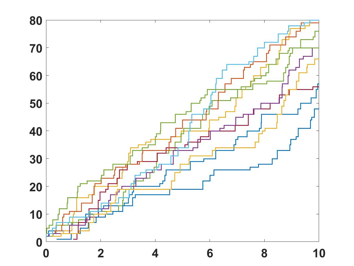
(a) Parameters: $k=3$

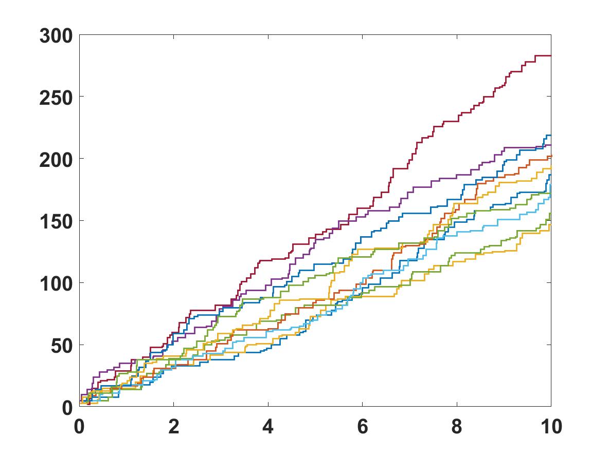
(b) Parameters: $k=5$

Figure 1. Ten simulated sample paths of the PPoK process for order (A) $k=3$, and (B) $k=5$

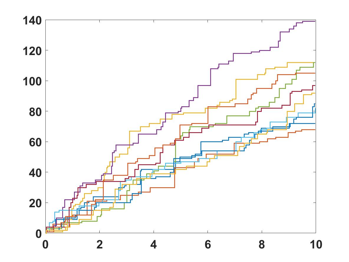
(a) Parameters: $\alpha=3.0,p=4.0,k=3$

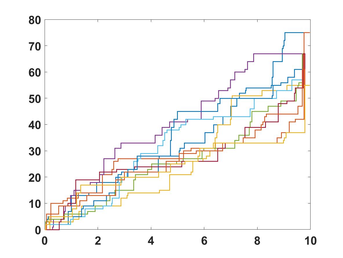
(b) Parameters: $\alpha=3.0,p=4.0,k=3$

Figure 2. Ten simulated sample paths of time-changed PPoK with (A) gamma subordinator, and (B) inverse gamma subordinator.

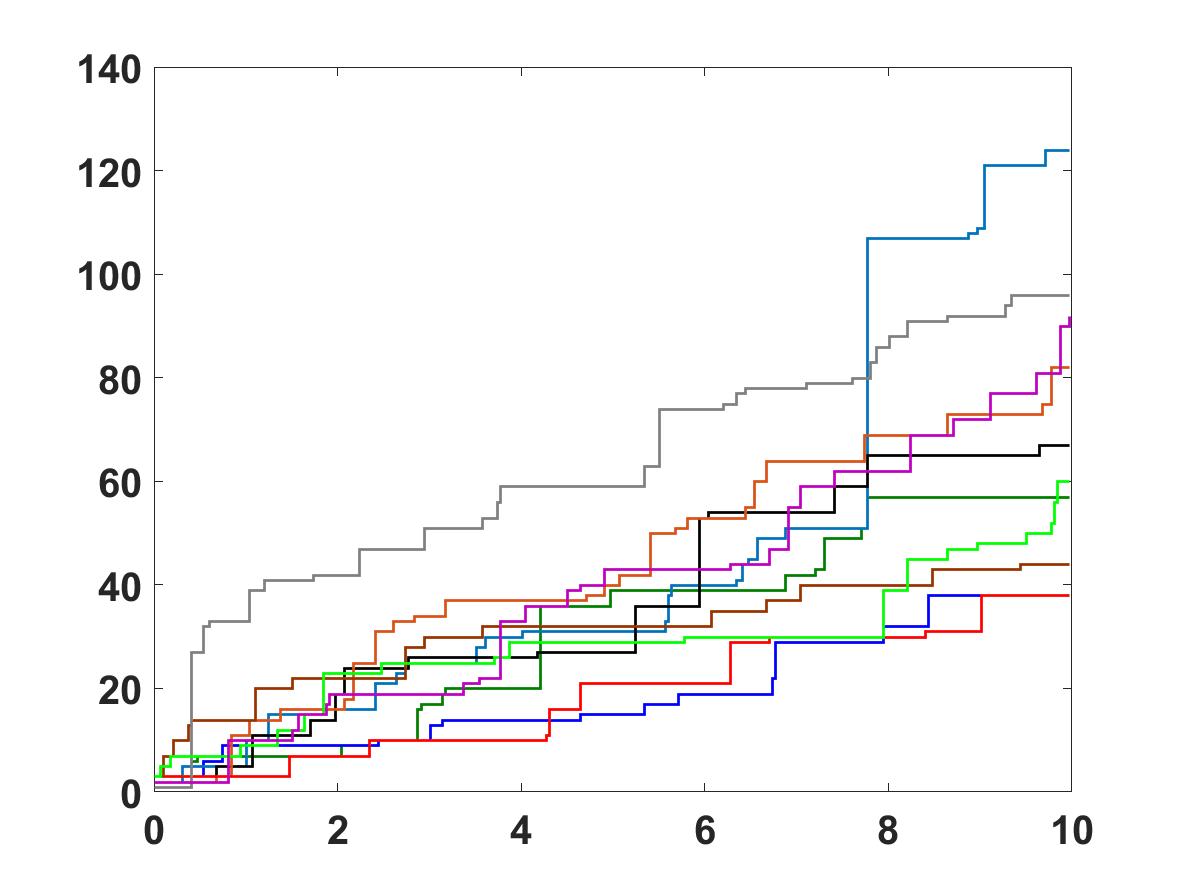
(a) Parameters: $\gamma=1,\delta=1,k=3$

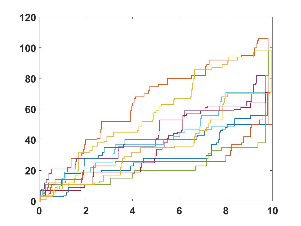
(b) Parameters: $\gamma=1,\delta=1,k=3$

Figure 3. Ten simulated sample paths time-changed PPoK with (A) inverse Gaussian subordinator, and (B) inverse of inverse Gaussian subordinator.

Interpretation of plots

The PPoK is interpreted as arrival coming in packets of size $k$. As it is clear from Figure 1, as the packet size $k$ is increased from 3 to 5, the number of arrivals increased. The effect of time-change by subordinator in PPoK is clearly visible in Figure 2(A) and 3(A) as the arrival rate of the packets increases compared with Figure 1(A). While if we observe the effect of inverse subordinator in 2(B) and 3(B), we find that the waiting time between events are increased predominantly compared to Figure 1(A).

References

• [1] H. Allouba. Brownian-time processes: the PDE connection. II. And the corresponding Feynman-Kac formula. Trans. Amer. Math. Soc., 354(11):4627–4637 (electronic), 2002.
• [2] H. Allouba and W. Zheng. Brownian-time processes: the PDE connection and the half-derivative generator. Ann. Probab., 29(4):1780–1795, 2001.
• [3] D. Applebaum. Lévy Processes and Stochastic Calculus, volume 116 of Cambridge Studies in Advanced Mathematics. Cambridge University Press, Cambridge, second edition, 2009.
• [4] B. Baeumer, M. M. Meerschaert, and E. Nane. Brownian subordinators and fractional Cauchy problems. Trans. Amer. Math. Soc., 361(7):3915–3930, 2009.
• [5] O. E. Barndorff-Nielsen. Normal inverse Gaussian distributions and stochastic volatility modelling. Scand. J. Statist., 24(1):1–13, 1997.
• [6] O. E. Barndorff-Nielsen. Processes of normal inverse Gaussian type. Finance Stoch., 2(1):41–68, 1998.
• [7] L. Beghin and E. Orsingher. Fractional Poisson processes and related planar random motions. Electron. J. Probab., 14:no. 61, 1790–1827, 2009.
• [8] J. Bertoin. Lévy processes, volume 121 of Cambridge Tracts in Mathematics. Cambridge University Press, Cambridge, 1996.
• [9] S. Bochner. Diffusion equation and stochastic processes. Proceedings of the National Academy of Sciences of the United States of America., 35(7):368–370, 1949.
• [10] D. O. Cahoy, V. V. Uchaikin, and W. A. Woyczynski. Parameter estimation for fractional Poisson processes. J. Statist. Plann. Inference, 140(11):3106–3120, 2010.
• [11] L. Calvet, B. Mandelbrot, and A. J. Fisher. A multifractal model of asset returns. Working papers, HAL, 2011.
• [12] P. K. Clark. A subordinated stochastic process model with finite variance for speculative prices. Econometrica, 41(1):135–155, 1973.
• [13] R. Cont and P. Tankov. Financial modelling with jump processes. Chapman & Hall/CRC Financial Mathematics Series. Chapman & Hall/CRC, Boca Raton, FL, 2004.
• [14] M. M. Dacorogna, U. A. Müller, R. J. Nagler, R. B. Olsen, and O. V. Pictet. A geographical model for the daily and weekly seasonal volatility in the foreign exchange market. Journal of International Money and Finance, 12(4):413 – 438, 1993.
• [15] B. Dybiec and E. Gudowska-Nowak. Subordinated diffusion and continuous time random walk asymptotics. Chaos: An Interdisciplinary Journal of Nonlinear Science, 20(4):043129, 2010.
• [16] R. Failla, P. Grigolini, M. Ignaccolo, and A. Schwettmann. Random growth of interfaces as a subordinated process. Phys. Rev. E, 70:010101, Jul 2004.
• [17] I. Golding and E. C. Cox. Physical nature of bacterial cytoplasm. Phys. Rev. Lett., 96:098102, Mar 2006.
• [18] M. G. Hahn, K. Kobayashi, and S. Umarov. Fokker-Planck-Kolmogorov equations associated with time-changed fractional Brownian motion. Proc. Amer. Math. Soc., 139(2):691–705, 2011.
• [19] K. Y. Kostadinova and L. D.Minkova. On the Poisson process of order $k$. Pliska Stud. Math. Bulgar., 22, 2012.
• [20] A. Kumar, E. Nane, and P. Vellaisamy. Time-changed poisson processes. Statistics & Probability Letters, 81(12):1899 – 1910, 2011.
• [21] A. Kumar and P. Vellaisamy. Inverse tempered stable subordinators. Statistics & Probability Letters, 103:134 – 141, 2015.
• [22] N. Laskin. Fractional Poisson process. Commun. Nonlinear Sci. Numer. Simul., 8(3-4):201–213, 2003. Chaotic transport and complexity in classical and quantum dynamics.
• [23] A. Maheshwari and P. Vellaisamy. On the long-range dependence of fractional poisson and negative binomial processes. J. Appl. Probab., 53:989–1000, 2016.
• [24] A. Maheshwari and P. Vellaisamy. Fractional poisson process time-changed by lévy subordinator and its inverse. Journal of Theoretical Probability, Dec 2017.
• [25] B. B. Mandelbrot. Scaling in financial prices: I. tails and dependence. Quantitative Finance, 1(1):113–123, 2001.
• [26] C. Marinelli, S. Rachev, and R. Roll. Subordinated exchange rate models: evidence for heavy tailed distributions and long-range dependence. Mathematical and Computer Modelling, 34(9):955 – 1001, 2001.
• [27] M. M. Meerschaert, T. J. Kozubowski, F. J. Molz, and S. Lu. Fractional Laplace model for hydraulic conductivity. Geophys. Res. Lett., 31:L08501, 2004.
• [28] M. M. Meerschaert, E. Nane, and P. Vellaisamy. The fractional Poisson process and the inverse stable subordinator. Electron. J. Probab., 16:no. 59, 1600–1620, 2011.
• [29] M. G. Nezhadhaghighi, M. A. Rajabpour, and S. Rouhani. First-passage-time processes and subordinated schramm-loewner evolution. Phys. Rev. E, 84:011134, Jul 2011.
• [30] E. Orsingher and F. Polito. Compositions, random sums and continued random fractions of poisson and fractional poisson processes. Journal of Statistical Physics, 148(2):233–249, Aug 2012.
• [31] E. Orsingher and F. Polito. The space-fractional Poisson process. Statist. Probab. Lett., 82(4):852–858, 2012.
• [32] E. Orsingher and B. Toaldo. Counting processes with bernstein intertimes and random jumps. Journal of Applied Probability, 52(4):1028–1044, 2015.
• [33] A. N. Philippou. Poisson and compound poisson distributions of order k and some of their properties. Journal of Soviet Mathematics, 27(6):3294–3297, Dec. 1984.
• [34] A. N. Philippou, C. Georghiou, and G. N. Philippou. A generalized geometric distribution and some of its properties. Statistics & Probability Letters, 1(4):171 – 175, 1983.
• [35] K. Sato. Lévy Processes and Infinitely Divisible Distributions, volume 68 of Cambridge Studies in Advanced Mathematics. Cambridge University Press, Cambridge, 1999. Translated from the 1990 Japanese original, Revised by the author.
• [36] K.-i. Sato. Subordination and self-decomposability. Statist. Probab. Lett., 54(3):317–324, 2001.
• [37] H. Scher, G. Margolin, R. Metzler, J. Klafter, and B. Berkowitz. The dynamical foundation of fractal stream chemistry: The origin of extremely long retention times. Geophysical Research Letters, 29(5):5–1–5–4.
• [38] R. L. Schilling, R. Song, and Z. Vondraček. Bernstein functions, volume 37 of de Gruyter Studies in Mathematics. Walter de Gruyter & Co., Berlin, second edition, 2012. Theory and applications.
• [39] A. Stanislavsky and K. Weron. Two-time scale subordination in physical processes with long-term memory. Annals of Physics, 323(3):643 – 653, 2008.
• [40] M. Veillette and M. S. Taqqu. Numerical computation of first passage times of increasing Lévy processes. Methodol. Comput. Appl. Probab., 12(4):695–729, 2010.
• [41] P. Vellaisamy and A. Kumar. First-exit times of an inverse gaussian process. Stochastics, 90(1):29–48, 2018.
• [42] P. Vellaisamy and A. Maheshwari. Fractional negative binomial and Polya processes. Probab. Math. Statist., 38(1):77–101, 2018.