Photogalvanic currents in dynamically gapped Dirac materials
Abstract
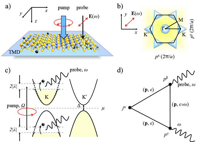
We develop a microscopic theory of an unconventional photogalvanic effect in two-dimensional materials with the Dirac energy spectrum of the carriers of charge under strong driving. As a test bed, we consider a layer of a transition metal dichalcogenide, exposed to two different electromagnetic fields. The first pumping field is circularly-polarized, and its frequency exceeds the material bandgap. It creates an extremely nonequilibrium distribution of electrons and holes in one valley (K) and opens dynamical gaps, whereas the other valley (K′) remains empty due to the valley-dependent interband selection rules. The second probe field has the frequency much smaller than the material bandgap. It generates intraband perturbations of the nonequilibrium carriers density, resulting in the photogalvanic current due to the trigonal asymmetry of the dispersions. This current shows thresholdlike behavior due to the dynamical gap opening and renormalizations of the density of states and velocity of quasiparticles.
I I. Introduction
Two-dimensional (2D) quantum systems exposed to external powerful high-frequency electromagnetic (EM) fields exhibit a variety of fascinating phenomena Ivchenko , including dissipation-free electron transport KibisPRL , quasi-condensation ExPol1 ; ExPol2 , and the photon drag effect Wieck ; Glazov ; Entin ; RefRPQ among others. In the case of nearly-resonant excitation of a solid-state system and strong light-matter interaction, it is convenient to work with hybrid photon-dressed quasiparticles, characterized by nonequilibrium steady-state distribution functions OurNJP . Their spectrum possesses a dynamical gap OurNJP ; ShelykhGap ; Machlin , determined by the amplitude of the external EM field BlochOsc .
Initially, dynamical gaps were studied in gapless materials such as graphene Geim ; RefSyzranov1 ; RefSyzranov2 . Currently, valley physics of 2D materials xiao2007valley , in particular transition metal dichalcogenides (TMDs) jung2015origin ; xu2014spin , is in focus yao2008valley . Their Brillouin zone contains two valleys K and K′, coupled by the time reversal symmetry. Therefore in addition to momentum and spin, 2D semiconductors possess another degree of freedom, which refers to particular valley. It is especially practical, that spectrum of TMDs has large gap (e.g., in MoS2 it amounts to xiao2012coupled ), giving a possibility to study valley-resolved physics RefMak ; RefUbrig .
They have symmetry properties similar to monolayer graphene with staggered sublattice potential. Due to the spatial inversion symmetry breaking, there occur transport effects described by a third-order generalized conductivity tensor. A typical example is the photogalvanic effect (PGE) also called the photovoltaic effect, where the components of photoinduced current are coupled with the components of the vector potential of an external EM field by the relation
| (1) |
where and is the photogalvanic third-order tensor, which can only exist (be finite) in noncentrosymmetric materials.
The microscopic origin of the conventional PGE is in the asymmetry of the interaction potential or the crystal-induced Bloch wave function ivchenko ; belinicher . It can also take place in 2D materials. However, there can appear an unconventional PGE due to the trigonal warping of the valleys. This asymmetry of the particle dispersion leads to such fascinating phenomena as the second harmonic generation GT , purely valley currents MEGT and alignment of the photoexcited carriers in gapless materials Portnoi1 ; Portnoi2 . Recently, the PGE produced by a weak EM fields and the spectrum warping of the valleys have also been discussed MagarillEntinKovalev .
The PGE currents in valleys K and K′ flow in opposite directions. Consequently, the net current is zero due to the time reversal symmetry. To launch a nonzero current in such circumstances, one has to break the time reversal symmetry. It can be done by an external electromagnetic field with circular polarization. Indeed, the specific property of TMD materials is that they possess the polarization-sensitive interband optical selection rules: electrons in the valley K (K′) couple with light and perform an interband transition only if the polarization of light coincides with the valley K (K′) chirality. This selection rule originates from the band topology of the Hamiltonian, reflecting the opposite Berry curvatures at K and K′ and resulting in a disbalance of electron populations in the two valleys (and the anomalous Hall effect Karch ). The linear-response perturbation theory of light-matter coupling in TMDs has been developed in a number of works gibertini2014spin ; Li ; Rostrami . However, nonlinear optical phenomena NLBoyd remain largely unexplored NLDirac1 ; NLDirac2 .
In this manuscript, we demonstrate that an unconventional PGE can occur in a 2D material if the valleys have different populations since the system is exposed to strong circularly-polarized light. The monolayer is initially non-conducting since the conductivity bands of both the valleys are empty. We expose the system to two EM fields. The first pumping circularly-polarized EM field with strong intensity populates one of the valleys, whereas the other valley remains empty. Due to the intravalley scattering, the valley reaches the saturation regime, when all the energy states in the valley are populated below some energy, which is determined by the EM field frequency. This regime is characterized by first, strong stationary nonequilibrium electron distribution function and second, strong modification of the energy spectrum of photogenerated electrons. The intraband dynamical gap opens, and its size is determined by the intensity of the pump EM field. The second probe linearly-polarized EM field opens the intraband transitions, resulting in the uncompensated PGE current.
II II. Theory
The system schematic is presented in Fig. 1(a). To describe it, we start with the Hamiltonian in the electron representation:
| (2) |
where the energy is counted from the middle of the TMD layer bandgap and is the momentum; we assume equal electron effective masses in the conduction and valence bands , and we disregard the spin-orbit splitting of the valence band; are the trigonal valley warping corrections to the electron dispersion in the corresponding bands [see Fig. 1(b)], , is a valley index, and the parameters describe the strength of the warping.
The external EM fields acting on the monolayer are introduced by the Pierls’ rule and the total Hamiltonian reads
| (5) |
where is the interband matrix element of the pump field with frequency [see Fig. 1(c)]. Within the parabolic band approximation, the matrix element possesses the following property: , reflecting the valley selective optical interband transitions under the pump EM field with circular polarization and intensity OurNJP ; is the vector potential of the probe EM field, is a Pauli matrix.
The current density operator reads , thus , where is the lesser Green’s function. Here and below we use the upper index to indicate the Cartesian components and the lower index to indicate the matrix elements. Figure 1(d) shows the Feynman diagrams, which we use to find the current density. The probe field is assumed to be weak, hence to calculate the PGE current we use the second-order response theory:
| (6) | |||
Here is the Keldysh contour. After some derivations, Eq. (6) gives two terms. The first one is time-independent, it describes the stationary PGE current. The second term contains the double frequency of the probe field, describing the second harmonic generation phenomena, which is beyond the scope of this manuscript.
The pump field should be taken into account in a nonperturbative manner. Thus the Green’s functions in Eq. (6) depend on the times separately:
| (9) |
where for convenience we denoted . The Green’s funciton in Eq. (9) can be easily found using a unitary transformation to the rotating frame by the operator , yielding:
| (12) |
where
| (17) |
and
| (20) | |||
Here are dispersions of quasiparticles in the presence of resonant pumping EM field, and is a momentum relaxation time.
Using the linearly-polarized probe field c.c. and applying the Keldysh diagrammatic technique Keldysh , we find
| (21) | |||
where is the nonequilibrium quasiparticle distribution function (as opposed to equilibrium electron distribution). In general case it depends on the intensity of the pump EM field, intraband relaxation, interband recombination, and intervalley scattering times OurNJP . As it follows from Eq. (21), the contributions of electrons from the conduction and valence bands have similar structure and they sum up. Thus, we can consider only one of the bands and after extend the results on the other band.
III III. Results and discussion
The action of the pump field not only results in the population of the valley, but also opens a dynamical gap in quasiparticle dispersion, see Eq. (20) and Fig. 1(c). Obviously, the PGE current at occurs only if . We consider here quasiballistic electron motion, assuming that the scattering is weak enough (or the intensity of the pump field is strong enough), so that .
Combining together Eqs. (17), (20) and (21), the conduction band contribution to the PGE tensor reads
The valence band contribution can be found from Eq. (III) by the replacement .
The intraband kinetics of photogenerated electrons under the action of resonant pump field has been considered in Refs. OurNJP, ; elesin1971coherent, ; Galitskii, . It was shown that if the intraband relaxation time is much smaller than the interband recombination time (saturation regime), then the distribution function of the quasiparticles with the dispersions (20) has the form of the Fermi distribution with zero Fermi energy Remark_Elesin , . In the limit of zero temperature, .
As it has been pointed out above, the PGE comes from the trigonal warping of the electron spectrum. Due to the smallness of this effect, we expand the current up to the linear-order corrections in and . These warping terms are contained in the coefficients and in the quasiparticle dispersions . Expanding Eq. (III) and combining the contributions from the conduction and valence bands, we find
| (23) | |||
where
| (24) | |||
Here is the quasiparticle dispersion in the absence of warping. If the frequency of the pump field satisfies , then instead of the integration over the momentum in (24) we can perform the -integration, replacing
The analysis of Eq. (23) shows that the nonzero elements of PGE tensor read
| (25) |
that allows us to find all the components, calculating only the component. Performing the integration in Eq. (23), we find (restoring the Plank constant):
| (26) | |||
where . We see that the current is proportional to , which determines the sensitivity of the current to valley quantum number, polarization of the pump EM field, and the factor .
It should be noted, that here we derived the expression for the PGE tensor in the case when the TMD layer is initially in the dielectic regime with the chemical potential lying in the bandgap. The generalization for the case of n- or p-doped TMDs can be done by replacing with its value shifted by the Fermi energy. We have disregarded here the possible spin splitting of the bands. The spin quantum number should be conserved in the interband optical transitions, and the respective contributions to the PGE current are just summed up.
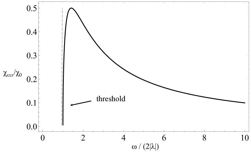
Figure 2 shows the spectrum of . The qualitative explanation of such dependence of the current on the frequency is the following. In the vicinity of the dynamical-induced gap, the density of states (DOS) is renormalized. Indeed, using the standard formula
| (27) |
we find
| (28) |
where is the DOS of the 2D system in the absence of a pump. We see that DOS (28) drastically increases in the vicinity of dynamical bandgap . At the same time, the velocity of quasiparticles is zero at , suppressing the PGE current at the threshold. Thus, the quasi-resonant behavior of PGE current in Fig. 2 is the combined effect of these two factors.
Conclusions
We have developed a microscopic quantum theory of an unconventional photogalvanic effect in 2D Dirac semiconductors under the action of strong pumping electromagnetic field. We have demonstrated, that the emergence of photon-dressed quasiparticles and the dynamical gap opening result in a thresholdlike behavior of the current as a function of the probe field frequency due to the dynamical renormalization of the density of states and quasiparticle velocity.
Our results can be extended to other materials, possessing a similar band structure as TMDs and obeying the valley-dependent interband optical selection rules. Moreover, the appearance of dynamically-induced gaps and the renormalization of the density of states open a way for engineering dispersions of quasiparticles in order to affect valley-selective second-order response effects, such as the photon drag effect and, possibly, the second harmonic generation.
Acknowledgments
We acknowledge stimulating discussions with M. Entin. We also thank E. Savenko for the help with the figures. This research has been supported by the Russian Science Foundation (Project No. 17-12-01039) and the Institute for Basic Science in Korea (Project No. IBS-R024-D1).
References
- (1) E. L. Ivchenko, Optical spectroscopy of semiconductor nanostructures (Alpha Science, Harrow, UK, 2005).
- (2) O. Kibis, Dissipationless Electron Transport in Photon-Dressed Nanostructures, Phys. Rev. Lett. 107, 106802 (2011).
- (3) J. Kasprzak, M. Richard, S. Kundermann, A. Baas, P. Jeambrun, J. M. J. Keeling, F. M. Marchetti, M. H. Szymanska, R. André, J. L. Staehli, V. Savona, P. B. Littlewood, B. Deveaud, and L. S. Dang, Bose Einstein condensation of exciton polaritons, Nature (London) 443, 409 (2006).
- (4) A. V. Kavokin, J. J. Baumberg, G. Malpuech, and F. P. Laussy, Microcavities (Oxford University Press, New York, 2006).
- (5) A. D. Wieck, H. Sigg, and K. Ploog, Observation of resonant photon drag in a two-dimensional electron gas, Phys. Rev. Lett. 64, 463 (1990).
- (6) M. M. Glazov, S. D. Ganichev, High frequency electric field induced nonlinear effects in graphene, Phys. Rep. 535, 101 (2014).
- (7) M. V. Entin, L. I. Magarill, and D. L. Shepelyansky, Theory of resonant photon drag in monolayer graphene, Phys. Rev. B 81, 165441 (2010).
- (8) V. M. Kovalev, A. E. Miroshnichenko, and I. G. Savenko, Photon drag in Bose-Einstein condensates, Phys. Rev. B 98, 165405 (2018); M. V. Boev, V. M. Kovalev, I. G. Savenko, Resonant photon drag of dipolar excitons, JETP Lett. 107, 763 (2018); V. M. Kovalev, M. V. Boev, I. G. Savenko, Proposal for frequency-selective photodetector based on the resonant photon drag effect in a condensate of indirect excitons, Phys. Rev. B 98, 041304(R) (2018).
- (9) V. M. Kovalev, W.-K. Tse, M. V. Fistul, and I. G. Savenko, Valley Hall transport of photon-dressed quasiparticles in two-dimensional Dirac semiconductors, New J. Phys. 20, 083007 (2018).
- (10) O. V. Kibis, K. Dini, I. V. Iorsh, and I. A. Shelykh, All-optical band engineering of gapped Dirac materials, Phys. Rev. B 95, 125401 (2017).
- (11) J. Tuorila, M. Silveri, M. Sillanpää, E. Thuneberg, Yu. Makhlin, and P. Hakonen, Stark effect and generalized Bloch-Siegert shift in a strongly driven two-level system, Phys. Rev. Lett. 105, 257003 (2010).
- (12) L. Allen and J. H. Eberly, Optical Resonance and Two-Level Atoms (Dover Publications, 1987).
- (13) K. S. Novoselov, A. K. Geim, S. V. Morozov, D. Jiang, M. I. Katsnelson, I. V. Grigorieva, S. V. Dubonos and A. A. Firsov, Two-dimensional gas of massless Dirac fermions in graphene, Nature (London) 438, 197-200 (2005).
- (14) S. V. Syzranov, Ya. I. Rodionov, K. I. Kugel, F. Nori, Strongly anisotropic Dirac quasiparticles in irradiated graphene, Phys. Rev. B 88(24) 241112 (2013).
- (15) Ya. I. Rodionov, K. I. Kugel, and F. Nori, Floquet spectrum and driven conductance in Dirac materials: Effects of Landau-Zener-Stückelberg-Majorana interferometry, Phys. Rev. B 94 195108 (2016).
- (16) D. Xiao, W. Yao, and Q. Niu, Valley-Contrasting Physics in Graphene: Magnetic moment and topological transport, Phys. Rev. Lett. 99, 236809 (2007).
- (17) J. Jung, A. DaSilva, A. H. MacDonald, and S. Adam, Origin of band gaps in graphene on hexagonal boron nitride, Nature Comm. 6, 6308 (2015).
- (18) X. Xu, W. Yao, D. Xiao and T. F. Heinz, Spin and pseudospins in layered transition metal dichalcogenides, Nature Phys. 10, 343 (2014).
- (19) W. Yao, D. Xiao, and Q. Niu, Valley-dependent optoelectronics from inversion symmetry breaking, Phys. Rev. B 77, 235406 (2008).
- (20) D Xiao, G.-B. Liu, W. Feng, X. Xu, and W. Yao, Coupled Spin and Valley Physics in Monolayers of MoS2 and Other Group-VI Dichalcogenides, Phys. Rev. Lett. 108, 196802 (2012).
- (21) K. F. Mak, K. L. McGill, J. Park, P. L. McEuen, The valley Hall effect in MoS2 transistors, Science 344(6191), 1489 (2014).
- (22) N. Ubrig, S. Jo, M. Philippi, D. Costanzo, H. Berger, A. B. Kuzmenko, and A. F. Morpurgo, Microscopic origin of the valley Hall effect in transition metal dichalcogenides revealed by wavelength-dependent mapping, Nano Lett. 17, 5719 (2017).
- (23) E. L. Ivchenko and G. E. Pikus, in: Problemy Sovremennoi Fiziki (Nauka, Leningrad, 1980), pp. 275-293.
- (24) V.I. Belinicher, B.I. Sturman, The photogalvanic effect in media lacking a center of symmetry Sov. Phys. Usp. 23 199 (1980).
- (25) L. E. Golub and S. A. Tarasenko, Valley polarization induced second harmonic generation in graphene, Phys. Rev. B 90, 201402(R) (2014).
- (26) L. E. Golub, S. A. Tarasenko, M. V. Entin and L. I. Magarill, Valley separation in graphene by polarized light, Phys. Rev. B 84, 195408 (2011).
- (27) R. R. Hartmann and M. E. Portnoi, Optoelectronic Properties of Carbon-based Nanostructures: Steering electrons in graphene by electromagnetic fields (LAP LAMBERT Academic Publishing, Saarbrucken, 2011).
- (28) V. A. Saroka, R. R. Hartmann, M. E. Portnoi, arXiv:1811.00987 (2018).
- (29) L. I. Magarill, M. V. Entin and V. M. Kovalev, arXiv:1811.01187 (2018).
- (30) J. Karch, P. Olbrich, M. Schmalzbauer, C. Zoth, C. Brinsteiner, M. Fehrenbacher, U. Wurstbauer, M. M. Glazov, S. A. Tarasenko, E. L. Ivchenko, D. Weiss, J. Eroms, R. Yakimova, S. Lara-Avila, S. Kubatkin, and S. D. Ganichev, Dynamic Hall effect driven by circularly polarized light in a graphene layer, Phys. Rev. Lett. 105, 227402 (2010).
- (31) M. Gibertini, F. M. D. Pellegrino, N. Marzari, and M. Polini, Spin-resolved optical conductivity of two-dimensional group-VIB transition-metal dichalcogenides, Phys. Rev. B 90, 245411 (2014).
- (32) Z. Li and J. P. Carbotte, Longitudinal and spin-valley Hall optical conductivity in single layer MoS2, Phys. Rev. B 86, 205425 (2012).
- (33) H. Rostami and R. Asgari, Intrinsic optical conductivity of modified Dirac fermion systems, Phys. Rev. B 89, 115413 (2014).
- (34) R. W. Boyd, Nonlinear Optics (Academic Press, 2003).
- (35) A. Saynatjoki, L. Karvonen, H. Rostami, A. Autere, S. Mehravar, A. Lombardo, R. A. Norwood, T. Hasan, N. Peyghambarian, H. Lipsanen, K. Kieu, A. C. Ferrari, M. Polini, and Z. Sun, Ultra-strong nonlinear optical processes and trigonal warping in MoS2 layers, Nature Comm. 8, 893 (2017).
- (36) R. A. Muniz and J. E. Sipe, All-optical injection of charge, spin, and valley currents in monolayer transition-metal dichalcogenides, Phys. Rev. B 91, 085404 (2015).
- (37) L. V. Keldysh, Diagram technique for nonequilibrium processes, JETP 20(4), 1018 [ZhETF 47(4), 1515] (1965).
- (38) V. F. Elesin, Coherent interaction of electrons of a semiconductor with a strong electromagnetic wave, Sov. Phys.-JETP 32, 328 (1971).
- (39) V. M. Galitskii, S. P. Goreslavskii, and V. F. Elesin, Electric and magnetic properties of a semiconductor in the field of a strong electromagnetic wave, Sov. Phys.-JETP 30, 117 (1970).
- (40) The results found in Refs. Galitskii ; elesin1971coherent are also applicable to 2D systems since the expressions of the electron distribution functions obtained in those works do not depend on the dimension of the system.