Magnetostatic interaction between two Bubble Skyrmions

Abstract

A detailed analytic and numerical analysis of the interaction between two bubble skyrmions has been carried out. Results from micromagnetic calculations show a strong dependence of the parameters of the skyrmion magnetic profile as a function of the magnetostatic interaction. The magnetic core and edge-width sizes of the skyrmion increase or decrease depending on the relative position between the skyrmions and the uniaxial perpendicular anisotropy. In particular, when a magnetic disk is over another, there is a transition from a Bloch-like skyrmion configuration to a Néel-like skyrmion configuration as the distance between the disks decreases, as a consequence of the magnetostatic interaction. Therefore, it is possible to stabilize a bubble skyrmion with a Néel configuration without the Dzyaloshinskii-Moriya interaction. Thus, these results can be used for the parameters control of the skyrmions in magnetic spintronic devices that need to use these configurations.

Introduction

During the last decade, a great deal of attention has been focused on the study of the magnetic skyrmions in magnetic structures because they have potential applications in magnetic storage devices of high density, spintronic devices, etc. [1, 2, 3, 4, 5, 6]. For example, in nanostructures such as nanodisks it is possible to find different type of skyrmions, like Néel, Bloch or bubble configurations, among others. The Néel and Boch skyrmion configurations can be obtained by introducing a Dzyaloshinskii-Moriya interaction due to the strong spin-orbit coupling between two materials [1, 2, 4, 7]. Similarly, the bubble skyrmions can be stabilized through an uniaxial magnetic anisotropy perpendicular to the plane of the disk [8, 9, 10, 11, 12].

It is interesting to note that the magnetic particles possess a long-range magnetostatic field, which is present in the formation of a great variety of magnetic textures like vortices or skyrmions. Recently, arrays of bubble skyrmions in nanodisks with perpendicular anisotropy have been proposed for the implementation of spintronic devices [13, 14, 15, 16]. In these systems, it should be emphasized that the interaction between the skyrmions through the magnetostatic field can be strong depending on their locations [2, 17]. In terms of analysis, the interaction between bubble skyrmions can be decomposed as the magnetostatic field interaction of cores and edges. This magnetostatic interaction could even influence their movements and may also affect their magnetic structures [17, 18] affecting the operation of the device. Therefore it becomes necessary to study in detail the interaction between two bubble skyrmions.

Hence, in this paper, we study the magnetostatic interaction between two magnetic dots that have a magnetic bubble skyrmion. They are stabilized by an effective anisotropy without the Dzyaloshinskii-Moriya interaction. Specifically, we focus our attention on the skyrmion core and edge that vary in size as a function of the magnetostatic interaction between these two magnetic dots. Based on micromagnetic calculations and micromagnetic simulations, we have carried out numerical calculations, in which we have observed a strong variation of the parameters of the skyrmion magnetic profile. The magnetic core and the edge-width sizes of the skyrmion increase or decrease depending on the relative position between the skyrmions and the uniaxial perpendicular anisotropy. In particular, it is possible to stabilize bubble skyrmions with a Néel-like skyrmion magnetic profile when a magnetic disk is over another, in the absence of the Dzyaloshinskii-Moriya interaction. This transition from the Bloch-like skyrmion configuration to the Néel-like skyrmion configuration is due to the magnetostatic interaction between the magnetic disks. These results could be useful for the realization of future bubble skyrmion devices.

Theory

We start with two dots that have a magnetic Co/Pt bubble skyrmion configuration. These dots are separated, center to center, by a horizontal distance $x$ and a vertical distance $z$, as shown in Fig. 1. The skyrmions are then allowed to interact through the magnetostatic interaction. Each magnetic dot has a radius $R$, a height $H$, and an effective magnetic uniaxial anisotropy perpendicular to the plane of the dot characterized by $K_{u}>0$. The magnetic parameters for each dot are $M_{s}=500$ kA/m and $A=1.5\times 10^{-11}$ J/m, so that the exchange length is equal to $L_{\text{ex}}=\sqrt{2A/\mu_{0}M_{s}^{2}}\approx 9.8$ nm [19]. We approach the study of these systems with the micromagnetic theory by using analytical and numerical calculations, and micromagnetic simulations.

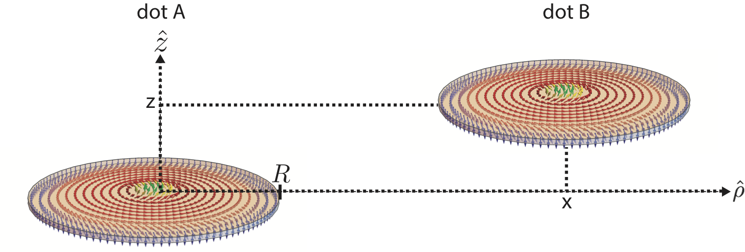
Figure 1: Schematic representation of two bubble skyrmions separated, center to center, by a horizontal distance $x$ and a vertical distance $z$. They are coupled by the magnetostatic interaction.

The micromagnetic simulations are performed with the Object Oriented Micromagnetic Framework (OOMMF) code [20]. We consider that each dot has a thickness $H=10$ nm and a radius $R=300$ nm, a cubic mesh size of $2\times 2\times 2$ nm³ and the Gilbert damping constant equal to $0.5$. To obtain the minimum energy configuration, we consider different initial states of the magnetization such as vortex, in plane, out of plane, and skyrmion configurations. To relax the system into the most stable configuration, we use the Euler method.

0.1 Horizontal separation between two magnetic disks with low anisotropy

In the first place, we consider two disks, with low magnetic anisotropy, separated by a horizontal distance ($x>R$) and in the same plane ($z=0$). From the micromagnetic simulations, we propose a magnetic profile of the form of a Bloch-like skyrmion characterized by a magnetization that rotates in the plane and perpendicular to the radial direction, i.e., $\vec{M}\left(\vec{r}\right)=M_{s}[m_{\phi}\left(\rho\right)\hat{\phi}+m_{z}\left(\rho\right)\hat{z}]$, where $M_{s}$ is the saturation magnetization of the dot, and $m_{\phi}^{2}(\rho)+m_{z}^{2}(\rho)=1$. Then, the analytical and numerical calculations are done by parameterizing the magnetization function for the bubble skyrmion in cylindrical coordinates by [21, 12]

$$m_{z}^{B_{1}}(\rho)=\left\{\begin{matrix}\delta+\left(1-\delta\right)\left(1-\dfrac{\rho^{2}}{\alpha^{2}}\right)^{4}&0<\rho\leq\alpha\\ \delta&\alpha<\rho\leq\beta\\ \delta-g\left(1+\delta\right)\left(1-\dfrac{(R-\rho)^{2}}{(R-\beta)^{2}}\right)^{4}&\beta<\rho\leq R\end{matrix}\right.$$ (1)

where $g$ is a parameter related to the maximum value of the $z$ component of the magnetization in the edge of the disk and takes the value between 0 and 1. $\delta$ is related to the plateau of the $z$ component of the magnetization observed in the OOMMF simulations. $\alpha$ and $\beta$ are related with the beginning and ending of the plateau, respectively [$m_{z}^{B_{1}}(\alpha)=m_{z}^{B_{1}}(\beta)=\delta$]. The abbreviation $B_{1}$ in the superindex of $m_{z}$ is used with the aim of referring to a Bloch-like skyrmion. Figure 2 illustrates the $z$-component of the magnetization of the magnetic profile for $K_{u}=143$ kJ/m³. The top row illustrates a comparison between the analytic magnetic profile given by Eq. (1) and the magnetic profile obtained by the micromagnetic simulation with OOMMF. The bottom row illustrates a top view of the magnetization obtained with OOMMF. Figures 2(a) and 2(d) considers an isolated magnetic dot. Figures 2(b) and 2(e) considers the strongest magnetostatic interaction between two disks with a parallel-configuration of the magnetic bubbles with $x=610$ nm that we have studied. Figures 2(c) and 2(f) considers the strongest magnetostatic interaction between two disks with an anti parallel-configuration of the magnetic bubbles with $x=610$ nm that we have studied. The analytical magnetic profile shows a very good agreement with the micromagnetic simulations when the disk is isolated. We observe a difference between the analytical and numerical value where the $z$ component of the magnetization is equal to zero of approximately 6%. Therefore, these OOMMF simulations suggest that the cylindrical angular variation in the magnetic profile of these bubble skyrmions can be disregarded in first approach when they are interacting by the magnetostatic interaction, as suggest Figs. 2(d), 2(e), and 2(f). Hence, for simplicity, in the analytical analysis below we will consider that their magnetic profiles do not depend on the polar angle. Therefore, we use the magnetic profile given by Eq. (1) when $z=0$ and $K_{u}=143$ kJ/m³.

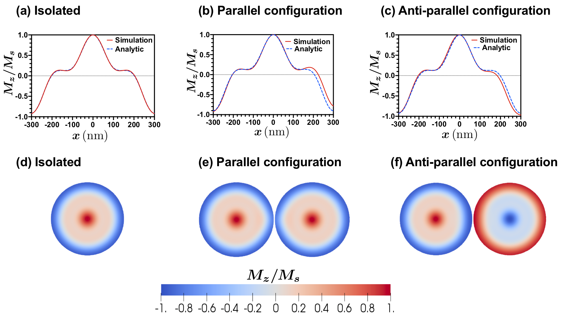
Figure 2: Comparison between the analytic magnetic profile given by Eq. (1) and the magnetic profile obtained by the micromagnetic simulation with OOMMF with $R=300$ nm, $H=10$ nm, $K_{u}=143$ kJ/m³, and $z=0$. Magnetic profile of (a) an isolated disk, (b) two parallel $B_{1}$ configuration with $x=610$ nm, and (c) two antiparallel $B_{1}$ configuration with $x=610$ nm. In addition, Figures 2(d), 2(e), and 2(f) show a top view of the minimum energy configuration obtained by OOMMF for the Figures 2(a), 2(b), and 2(c), respectively.

The total magnetic energy of two disks with the $B_{1}$ configuration, $E_{\text{tot}}^{B_{1}}$, is given by the sum of the exchange, magnetostatic, and anisotropy energies, whose forms are suggested by the micromagnetic theory[22]. The exchange energy for the bubble skyrmion with the $B_{1}$ configuration, $E_{\text{ex}}^{B_{1}}$, is given by [12]

$$E_{\text{ex}}^{B_{1}}=2\pi HA\left[\int_{0}^{\alpha}f_{1}(\rho)\rho d\rho+\left(1-\delta^{2}\right)\ln\left(\frac{\beta}{\alpha}\right)+\int_{\beta}^{R}f_{2}(\rho)\rho d\rho\right],$$ (2)

where $A$ is the stiffness constant. The functions $f_{1}(\rho)$ and $f_{2}(\rho)$ in Eq. (2) are

$$f_{1}(\rho)=\frac{1-\left[(1-\delta)\zeta_{1}^{4}(\rho)+\delta\right]^{2}}{\rho^{2}}+\frac{64(1-\delta)^{2}\rho^{2}\zeta_{1}^{6}(\rho)}{\alpha^{4}\left(1-\left[(1-\delta)\zeta_{1}^{4}(\rho)+\delta\right]^{2}\right)},$$ (3)

$$f_{2}(\rho)=\frac{1-\left[\delta-g(\delta+1)\zeta_{2}^{4}(\rho)\right]^{2}}{\rho^{2}}+\frac{64g^{2}(\delta+1)^{2}\left(1-\zeta_{2}(\rho)\right)\zeta_{2}^{6}(\rho)}{(R-\beta)^{2}\left(1-\left[\delta-g(\delta+1)\zeta_{2}^{4}(\rho)\right]^{2}\right)},$$ (4)

with $\zeta_{1}(\rho)=1-\rho^{2}/\alpha^{2}$ and $\zeta_{2}(\rho)=1-(R-\rho)^{2}/(R-\beta)^{2}$. The magnetostatic contribution is given by the self-magnetostatic interaction for every dot defined by $E_{\text{m,self}}$, and the magnetostatic interaction between the dots called $E_{\text{m,int}}$. The self magnetostatic interaction is $E_{\text{m,self}}=(\mu_{0}/2)\int\vec{M}(\vec{r})\cdot\vec{\nabla}U_{\text{self}}(\vec{r})dv$, where $U_{\text{self}}(\vec{r})$ is the magnetostatic potential in a dot due to the magnetization of the same magnetic dot[22]. Observing that there are not volumetric charges in the magnetic profile of Eq. (1) [$\vec{\nabla}\cdot\vec{M}(\vec{r})=0$], then $E_{\text{m,self}}$ has the form [12]

$$E_{\text{m,self}}^{B_{1}}=\pi\mu_{0}M_{s}^{2}\int_{0}^{\infty}dq\left[F_{1}\left(q\right)+F_{2}\left(q\right)\right]^{2}\left(1-e^{-qH}\right),$$ (5)

where $F_{1}\left(q\right)$ and $F_{2}\left(q\right)$ are

$$F_{1}\left(q\right)=F_{11}(q)J_{1}(q\beta)+F_{12}(q)J_{1}(q\alpha)+F_{13}(q)J_{2}(q\alpha),$$ (6)

$$F_{2}\left(q\right)=\int_{\beta}^{R}\rho J_{0}(q\rho)m_{z}^{B_{1}}(\rho)d\rho,$$ (7)

where $F_{11}(q)=\beta\delta/q$, $F_{12}(q)=384(\delta-1)\left(48-q^{2}\alpha^{2}\right)/(q^{7}\alpha^{5})$, and $F_{13}(q)=4608(\delta-1)\left(q^{2}\alpha^{2}-16\right)/(q^{8}\alpha^{6})$. The magnetostatic interaction between the two dots is given by $E_{\text{m,int}}=\mu_{0}\int\vec{M}(\vec{r})\cdot\vec{\nabla}U_{\text{int}}(\vec{r})dv$, where $U_{\text{int}}(\vec{r})$ is the magnetostatic potential in a dot due to the magnetization of the other magnetic dot[22]. Then $E_{\text{m,int}}$ with the magnetic profile given by Eq. (1) is equal to:

$$E_{\text{m,int}}^{B_{1}}\left(x,z\right)=-\pi\mu_{0}M_{s}^{2}\sigma_{A}\sigma_{B}\int_{0}^{\infty}dqJ_{0}(qx)\left[F_{1}\left(q\right)+F_{2}\left(q\right)\right]^{2}e^{-q(H+z)}g(q,H,z),$$ (8)

where the letters $A$ and $B$ represent the dot $A$ and the dot $B$, respectively. $\sigma_{A}$ and $\sigma_{B}$ take values $\pm 1$, and their values define if the magnetization profile is given by Eq. (1) (value $+1$) or minus the magnetization profile given by Eq. (1) (value $-1$). In essence we can parametrize the skyrmions with two orientations, namely, up or down. When $\sigma_{A}=\sigma_{B}$ the configuration is called parallel, and when $\sigma_{A}\neq\sigma_{B}$ the configuration is called anti-parallel. The function $g(q,H,z)$ is:

$$g(q,H,z)=\begin{cases}\left(1-2e^{qH}+e^{2qz}\right)&0\leq z<H\\ \left(e^{qH}-1\right)^{2}&z\geq H\end{cases}$$ (9)

The anisotropy contribution, $E_{\text{ani}}$, is given by $E_{\text{ani}}=-K_{u}\int m_{z}^{2}(\rho)dv$. Then, $E_{\text{ani}}$, with the magnetic profile given by Eq. (1), is [12]:

$$E_{\text{ani}}^{B_{1}}=-2\pi K_{u}H\left(\dfrac{\alpha^{2}}{18}-\dfrac{(R-\beta)^{2}g^{2}}{18}+\dfrac{32768}{109395}(R-\beta)g^{2}R+f_{3}(\delta)\right),$$ (10)

where $f_{3}(\delta)$ is equal to

$$f_{3}(\delta)=f_{31}\delta+f_{32}\delta^{2},$$ (11)

$$f_{31}=\left(-\frac{(R-\beta)^{2}g^{2}}{9}+\frac{(R-\beta)^{2}g}{5}+\frac{65536(R-\beta)g^{2}R}{109395}-\frac{256(R-\beta)gR}{315}+\frac{4\alpha^{2}}{45}\right),$$ (12)

$$f_{32}=\left(-\frac{(R-\beta)^{2}g^{2}}{18}+\frac{(R-\beta)^{2}g}{5}+\frac{32768(R-\beta)g^{2}R}{109395}-\frac{256(R-\beta)gR}{315}+\frac{R^{2}}{2}-\frac{13\alpha^{2}}{90}\right).$$ (13)

Hence, the expression of the total energy of the system is equal to

$$E_{\text{tot}}^{B_{1}}=2E_{\text{ex}}^{B_{1}}+2E_{\text{m,self}}^{B_{1}}+2E_{\text{ani}}^{B_{1}}+E_{\text{m,int}}^{B_{1}}.$$ (14)

This expression, Eq. (14), depends on the parameters $x$, $z$, $\delta$, $g$, $\alpha$, and $\beta$. Therefore, to obtain the energy of the system, we need to minimize $E_{\text{tot}}^{B_{1}}$ as a function of the parameters $\delta$, $g$, $\alpha$, and $\beta$; for a fixed $R$, $H$, $x$, $z$, and $K_{u}$.

0.2 Horizontal separation between two magnetic disks with high anisotropy

In this section we consider two disks, with high magnetic anisotropy, separated by a horizontal distance ($x>R$) and in the same plane ($z=0$). From the micromagnetic simulations, we propose a magnetic profile of the form $\vec{M}\left(\vec{r}\right)=M_{s}[m_{\phi}\left(\rho\right)\hat{\phi}+m_{z}\left(\rho\right)\hat{z}]$, where the magnetic profile for $m_{z}\left(\rho\right)$, is given by [8]

$$m_{z}^{B_{2}}(\rho)=\tanh\left(\frac{\rho-\gamma}{\Delta}\right),$$ (15)

where $b=\gamma$ and $c=R-\gamma$ are the core and the edge-width of the magnetic bubble skyrmion, respectively. The abbreviation $B_{2}$ in the superindex of $m_{z}$ is used with the aim of referring to a Bloch-like skyrmion configuration. Figure 3 illustrates the $z$-component of the magnetization of the magnetic profile for $R=300$ nm, $H=10$ nm, and $K_{u}=150$ kJ/m³. The top row illustrates a comparison between the analytic magnetic profile given by Eq. (15) and the magnetic profile obtained by the micromagnetic simulation with OOMMF. The bottom row illustrates a top view of the magnetization obtained with OOMMF. Figures 3(a) and 3(d) considers an isolated magnetic bubble. Figures 3(b) and 3(e) consider the magnetostatic interaction between two disks with a parallel-configuration of the magnetic bubbles with $x=610$ nm. Figures 3(c) and 3(f) consider the magnetostatic interaction between two disks with an anti parallel-configuration of the magnetic bubbles with $x=610$ nm. The analytical magnetic profile shows a very good agreement with the micromagnetic simulation when the disk is isolated. We observe a difference between the analytical and numerical value where the $z$ component of the magnetization is equal to zero of approximate 7%. Therefore, these OOMMF simulations suggest that the cylindrical angular variation in the magnetic profile of these bubble skyrmion can be disregarded when they are interacting by the magnetostatic interaction, as suggest Figs. 3(d), 3(e), and 3(f). Hence, for simplicity, in the analytical analysis below we will consider that their magnetic profiles do not depend on the polar angle. Therefore, we use the magnetic profile given by Eq. (15) when $z=0$ and $K_{u}=150$ kJ/m³.

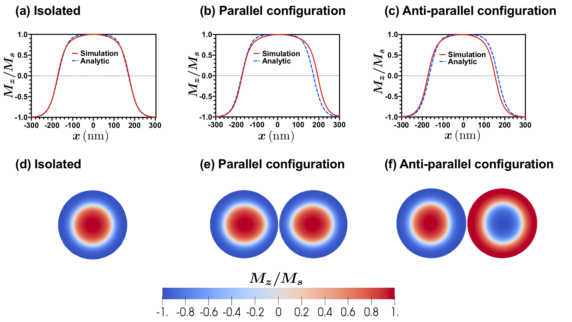
Figure 3: Comparison between the analytic magnetic profile given by Eq. (15) and the magnetic profile obtained by the micromagnetic simulation with OOMMF with $R=300$ nm, $H=10$ nm, $K_{u}=150$ kJ/m³, and $z=0$. Magnetic profile of (a) an isolated disk, (b) two parallel $B_{2}$ configuration with $x=610$ nm, and (c) two antiparallel $B_{2}$ configuration with $x=610$ nm. In addition, Figures 3(d), 3(e), and 3(f) show a top view of the minimum energy configuration obtained by OOMMF for the Figures 3(a), 3(b), and 3(c), respectively.

The total magnetic energy of the system with the $B_{2}$ configuration for the dots, $E_{\text{tot}}^{B_{2}}$, is given by the sum of the exchange, magnetostatic, and anisotropy energies, whose form are suggested by the micromagnetic theory[22]. The exchange energy for the bubble skyrmion configuration with the $B_{2}$ configuration, $E_{\text{ex}}^{B_{2}}$, is given by

$$E_{\text{ex}}^{B_{2}}=2\pi HA\int_{0}^{R}\frac{\left(\Delta^{2}+\rho^{2}\right)\operatorname{sech}^{2}\left(\frac{\gamma-\rho}{\Delta}\right)}{\Delta^{2}\rho^{2}}\rho d\rho.$$ (16)

The self-magnetostatic energy with the $B_{2}$ configuration is

$$E_{\text{m,self}}^{B_{2}}=\pi\mu_{0}M_{s}^{2}\int_{0}^{\infty}dq\left[\int_{0}^{R}J_{0}\left(q\rho\right)m_{z}^{B_{2}}(\rho)\rho d\rho\right]^{2}\left(1-e^{-qH}\right).$$ (17)

The magnetostatic interaction between the two dots is

$$E_{\text{m,int}}^{B_{2}}\left(x,z\right)=-\pi\mu_{0}M_{s}^{2}\sigma_{A}\sigma_{B}\int_{0}^{\infty}dqJ_{0}(qx)\left[\int_{0}^{R}J_{0}\left(q\rho\right)m_{z}^{B_{2}}(\rho)\rho d\rho\right]^{2}e^{-q(H+z)}g(q,H,z).$$ (18)

The anisotropy contribution is:

$$E_{\text{ani}}^{B_{2}}=-\pi HR^{2}K_{u}-2\pi HK_{u}\left(\Delta^{2}\ln\left[\cosh\left(\frac{\gamma-R}{\Delta}\right)\operatorname{sech}\left(\frac{\gamma}{\Delta}\right)\right]+\Delta R\tanh\left(\frac{\gamma-R}{\Delta}\right)\right).$$ (19)

Therefore, the total energy expression of the system with the $B_{2}$ configuration for the dots is equal to

$$E_{\text{tot}}^{B_{2}}=2E_{\text{ex}}^{B_{2}}+2E_{\text{m,self}}^{B_{2}}+2E_{\text{ani}}^{B_{2}}+E_{\text{m,int}}^{B_{2}}.$$ (20)

This expression, Eq. (20), depends on the parameters $x$, $z$, $\gamma$, and $\Delta$. Therefore, to obtain the energy of the system, we need to minimize $E_{\text{tot}}^{B_{2}}$ as a function of the parameters $\gamma$ and $\Delta$; for a fixed $R$, $H$, $x$, $z$, and $K_{u}$.

0.3 Vertical separation between two magnetic disks

In this section we consider two disks, separated by a vertical distance ($z>H$) and in the same axis ($x=0$). Our micromagnetic simulations show that the magnetic configuration of each dot changes from a Bloch-like skyrmion configuration to a Néel-like skyrmion configuration as the distance between the dots decreases. In a Néel-like skyrmion the magnetization rotates in the plane parallel to the radial direction, then we propose a magnetic profile of the form $\vec{M}_{A}\left(\vec{r}\right)=-M_{s}m_{\rho}\left(\rho\right)\hat{\rho}+M_{s}m_{z}\left(\rho\right)\hat{z}$ and $\vec{M}_{B}\left(\vec{r}\right)=M_{s}m_{\rho}\left(\rho\right)\hat{\rho}+M_{s}m_{z}\left(\rho\right)\hat{z}$, for the dot $A$ and for the dot $B$, respectively. We have that $m_{\rho}^{2}(\rho)+m_{z}^{2}(\rho)=1$ and $m_{z}\left(\rho\right)$ is given by Eq. (15). Figure 4 illustrates the $z$-component of the magnetization of the magnetic profile for $z=30$ nm and $K_{u}=150$ kJ/m³. Figure 4(a) illustrates a comparison between the analytic magnetic profile and the magnetic profile obtained by the micromagnetic simulation with OOMMF. Figure 4(b) shows a top view of the magnetization of the two dots. Figure 4(c) shows a schematic representation of the front view of the magnetization of both dots.

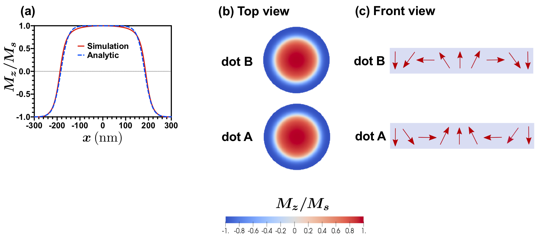
Figure 4: Magnetization of the minimum energy state for two dots, one over the other, with $R=300$ nm, $H=10$ nm, $K_{u}=150$ kJ/m³, $x=0$, and $z=30$ nm. (a) Comparison between the analytic magnetic profile of the Néel-like skyrmion configuration and the magnetic profile obtained by the micromagnetic simulation with OOMMF. (b) Top view of the magnetization obtained by OOMMF for the two dots. (c) Schematic representation of the front view of the magnetization of the two dots.

The total magnetic energy of the system with the Néel-like skyrmion configuration for the dots, $E_{\text{tot}}^{N}$, is given by the sum of the exchange, magnetostatic, and anisotropy energies. The abbreviation $N$ is used with the aim of referring to a Néel-like skyrmion. The exchange energy for the two dots with the $N$ configuration, $E_{\text{ex}}^{N}$, is the same given by the $B_{2}$ configuration, i.e., $E_{\text{ex}}^{N}=E_{\text{ex}}^{B_{2}}$. The self-magnetostatic energy in this case, comes from the superficial and volumetric magnetic charges. Then, the self-magnetostatic energy is:

$$E_{\text{m,self}}^{N}= \pi\mu_{0}M_{s}^{2}\ \int_{0}^{\infty}dq\left(qH+e^{-qH}-1\right)\left(\int_{0}^{R}m_{\rho}(\rho)J_{1}(q\rho)\rho d\rho\right)^{2}$$

$$+\pi\mu_{0}M_{s}^{2}\int_{0}^{\infty}dq\left(1-e^{-qH}\right)\left(\int_{0}^{R}m_{z}(\rho)J_{0}(q\rho)\rho d\rho\right)^{2}$$ (21)

The magnetostatic interaction between the two dots is equal to:

$$E_{\text{m,int}}^{N}\left(x=0,z\right)= -\pi\mu_{0}M_{s}\int_{0}^{\infty}dqe^{-q(H+y)}(e^{qH}-1)^{2}\left(\int_{0}^{R}m_{\rho}(\rho)J_{1}(q\rho)\rho d\rho\right)^{2}$$

$$-\pi\mu_{0}M_{s}\int_{0}^{\infty}dqe^{-q(H+y)}(e^{qH}-1)^{2}\left(\int_{0}^{R}m_{z}(\rho)J_{0}(q\rho)\rho d\rho\right)^{2}$$

$$-2\pi\mu_{0}M_{s}\int_{0}^{\infty}dqe^{-q(H+y)}(e^{qH}-1)^{2}\int_{0}^{R}m_{z}(\rho)J_{0}(q\rho)\rho d\rho\int_{0}^{R}m_{\rho}(\rho)J_{1}(q\rho)\rho d\rho.$$ (22)

The anisotropy contribution of the $N$ bubble skyrmion configuration is equal to the $B_{2}$ bubble configuration, i.e., $E_{\text{ani}}^{N}=E_{\text{ani}}^{B_{2}}$. Therefore, the total energy expression of the system with the $N$ configurations for the two dots at $x=0$ is equal to

$$E_{\text{tot}}^{N}=2E_{\text{ex}}^{N}+2E_{\text{m,self}}^{N}+2E_{\text{ani}}^{N}+E_{\text{m,int}}^{N}.$$ (23)

This expression, Eq. (23), depends on the parameters $x$, $z$, $\gamma$, and $\Delta$. Therefore, to obtain the energy of the system, we need to minimize $E_{\text{tot}}^{N}$ as a function of the parameters $\gamma$ and $\Delta$; for a fixed $R$, $H$, $x$, $z$, and $K_{u}$.

Results and Discussion

We start with two Co/Pt magnetic dots with geometrical parameters $R=300$ nm and $H=10$ nm. The center of the dot $A$ is set up at the origin $x=z=0$. With these parameters, we study two scenarios in the following subsections: the disks adjacent to each other is when the dot $B$ is at $x>2R$ and $z=0$ (dots in the same plane) and the disks vertically stacked corresponds to $x=0$ and $z>H$ (dots in the same axis $z$). In the following sections we study and discuss the magnetostatic interaction energy and also the dependence of the parameters of the skyrmion, the core size $b$ and the end-width size $c$, as a function of the distance between the dots. The analytical values for the core ($b_{a}$) and the end-width ($c_{a}$) sizes were obtained by minimizing the total magnetic energies given in the last section. The numerical values for the core ($b_{s}$) and the end-width ($c_{s}$) sizes were obtained by OOMMF simulations.

0.4 Horizontal separation between two magnetic disks with bubble skyrmion configurations, $x>2R$ and $z=0$.

In this section we study the magnetostatic interaction between two disks where the disks are one beside another, i.e., according to Fig. 1, $z=0$ and the distance between their centers is $x>2R$. Figure 5 illustrates the magnetostatic interaction energy normalized by $\mu_{0}M_{s}^{2}L_{\text{ex}}^{3}$, ${\cal{E}}_{\text{m,int}}=E_{\text{m,int}}/(\mu_{0}M_{s}^{2}L_{\text{ex}}^{3})$, as a function of $x$ for $K_{u}=$ $143$ kJ/m³ and $150$ kJ/m³. In this configuration, the magnetostatic interaction energy is negative when $\sigma_{A}\neq\sigma_{B}$, so that the two skyrmions are oriented antiparallel. Similar results were obtained with magnetic vortices in disks, where the antiparallel alignment of the vortices have the lowest magnetostatic energy [24, 25]. The orientation of the skyrmions is energetically favorable because the magnetic field lines produced at the edge of one of the skyrmions, can naturally and immediately match the orientation of the magnetization and magnetic field produced at the closest edge of the other skyrmion, minimizing the energy associated with the magnetostatic interaction (similar explanation is observed in two coupled vortices, where the magnetic cores close the magnetic field lines [24, 25]). For this reason, we start to analyze the antiparallel configuration in this subsection, as it corresponds to the configuration of lowest energy.

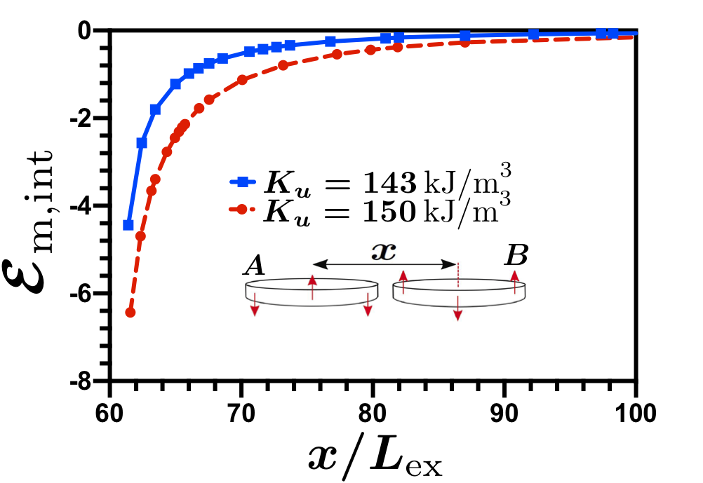
Figure 5: Normalized magnetostatic interaction energy as a function of the horizontal separation $x$ between the two disks with the antiparallel bubble skyrmion configurations for different anisotropies. The symbols represent the numerical points at different anisotropies. The lines are obtained by fitting these numerical points. The square (blue solid line) represents $K_{u}=143$ kJ/m³ and the dot (red dashed line) represents $K_{u}=150$ kJ/m³. Every disk has $h=10$ nm $/L_{\text{ex}}\approx 1.02$ and $r=300$ nm$/L_{\text{ex}}\approx 30.67$.

To study the dependence of the core size, $b$, and the edge-width size, $c$, of the two skyrmions as a function of $x$, we will choose the two following regimes. The first one is when $K_{u}=143$ kJ/m³ and we use the configuration $B_{1}$ [Eq. (1)]. The second one is when $K_{u}=150$ kJ/m³ and we use the configuration $B_{2}$ [Eq. (15)]. Figure 6 illustrates the parameters of the skyrmions, $b$ and $c$, as a function of $x$. Figure 6(a) considers $K_{u}=143$ kJ/m³ and Figure 6(b) considers $K_{u}=150$ kJ/m³. We observe a good agreement between the analytical calculation and the numerical simulations. When the distance between the disks decreases, the edge-width size of the skyrmions increases while the size of the cores decreases. This behavior can be explained by the following argument: when the two magnetic disks (skyrmions $A$ and $B$) are near each other, the magnetization directions for the edges of $A$ and $B$ are oriented antiparallel, allowing the magnetostatic field produce by one skyrmion to naturally close at the edge of the other skyrmion. This results in a decrease of the magnetostatic energy making the system to be more stable. When the skyrmions are close to each other, it is energetically favorable to have a relatively large edge $c$. However, when the disks are moved away from each other, the magnetostatic interaction between them is reduced compared to the other energy terms, so that $c$ begins to decrease until it reaches the value corresponding to an isolated skyrmion. In order to explain the behavior of the core of the skyrmion, we must first consider that the magnetic interaction between the core $A$ and the edge-width $B$ is stronger than the interaction between the core $A$ and the core $B$. This is because the magnetic volume due to the magnetization perpendicular to the plane of the disk from the cores is less than the magnetic volume from the the edge-widths, and also because the distance between the core $A$ and the core $B$ is greater than the distance between the core $A$ and the edge-width $B$. If we focus on the magnetic interaction between the core of the skyrmion $A$ and the edge-width of the skyrmion $B$ when they are close together, we see that both magnetization directions are the same. Such parallel configuration is not favorable, so that it is energetically favorable to have a small magnetic volume, i.e, the size of the core, $b$, should be small. For the purpose of increasing $b$, the magnetostatic interaction should diminish, therefore, we have to increase $x$. The opposite behavior occurs for the cores of the magnetic disk that have magnetic vortices, i.e., the core radius of the vortices decreases as the distance between them increases. This discussion for the vortices is analogous to what happens with the edges of the skyrmions, which correspond to the strongest interaction in this scenario, see Refs. [24, 25]. Analogously to the edge-width size, the core size of each skyrmion takes the value of an isolated disk when the separation distance is large enough to consider the magnetostatic interaction energy between the disks equal to zero.

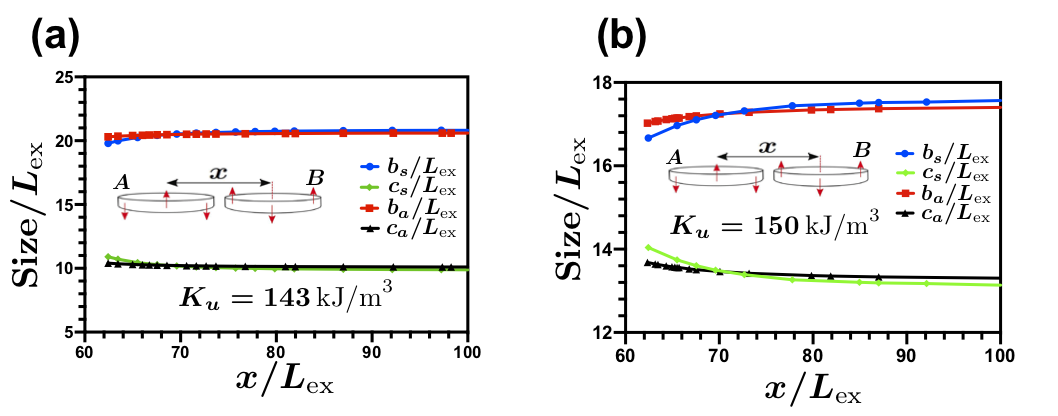
Figure 6: The core, $b$ ($b_{a}$ from the analytic model and $b_{s}$ from the micromagnetic simulations), and the edge-width, $c$ ($c_{a}$ from the analytic model and $c_{s}$ from the micromagnetic simulations), sizes of two disks with the antiparallel bubble skyrmion configurations as a function of $x$ at $h=10$ nm $/L_{\text{ex}}\approx 1.02$ and $r=300$ nm$/L_{\text{ex}}\approx 30.67$. The anisotropy is $(a)$ $K_{u}=143$ kJ/m³ and $(b)$ $K_{u}=150$ kJ/m³.

From an application point of view, both antiparallel and parallel configurations are well worth investigating, because the core orientation of the skyrmion can be used to encode binary information and could be either up or down, depending on the information. For this reason, in addition to the previous study of the antiparallel configuration, the parallel configuration of two skyrmions with a horizontal separation is investigated. Figure 7 illustrates the normalized magnetostatic interaction energy, as a function of $x$ for $143$ kJ/m³ and $150$ kJ/m³. In this configuration, the magnetostatic interaction energy is positive.

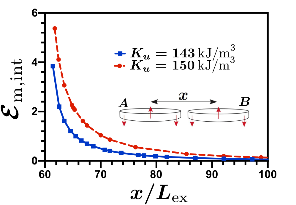
Figure 7: Normalized magnetostatic interaction energy as a function of the horizontal separation $x$ between the two disks with the parallel bubble skyrmion configurations for different anisotropies. The symbols represent the numerical points at different anisotropies. The lines are obtained by fitting these numerical points. The the square (blue solid line) represents $K_{u}=143$ kJ/m³ and the dot (red dashed line) represents $K_{u}$ =150 kJ/m³. Every disk has $h=10$ nm/$L_{\text{ex}}\approx 1.02$ and $r=300$ nm/$L_{\text{ex}}\approx 30.67$

Figure 8 illustrates the parameters of the skyrmions, $b$ and $c$, as a function of $x$. Figure 8(a) corresponds to $K_{u}=143$ kJ/m³ and Figure 8(b) corresponds to $K_{u}=150$ kJ/m³. In both cases, when the distance between the disks decreases, the edge-width size of the skyrmions decreases while the core size increases. We observe a good agreement between the analytical calculation and the numerical simulations. This can be explained through the core-edge and edge-edge interaction. The strongest interaction is between the edges and it is unfavorable, so the parameter $c$ decreases when $x$ decreases. On the another hand, the edge-core interaction is favorable, then the parameter $b$ increases when $x$ decreases.

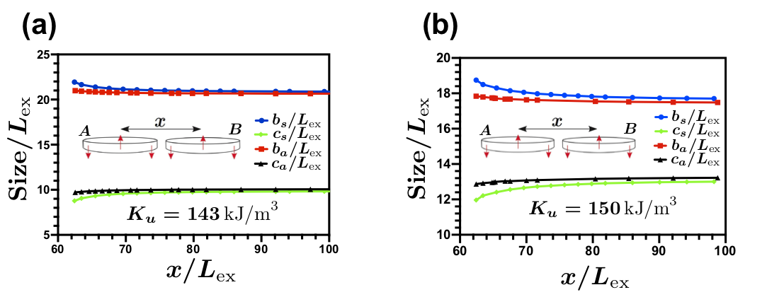
Figure 8: The core, $b$ ($b_{a}$ from the analytic model and $b_{s}$ from the micromagnetic simulations), and the edge-width, $c$ ($c_{a}$ from the analytic model and $c_{s}$ from the micromagnetic simulations), of two disks with the parallel bubble skyrmion configurations as a function of $x$ for $h=10$ nm/$L_{\text{ex}}\approx 1.02$ and $r=300$ nm/$L_{\text{ex}}\approx 30.67$. The anisotropy is (a) $K_{u}=143$ kJ/m³ and (b) $K_{u}=150$ kJ/m³.

0.5 Vertical separation between two magnetic disks with bubble skyrmion configurations, $x=0$ and $z>H$

In this section we study two disks where one disk is over the other, i.e., $x=0$ and $z>H$. To study the magnetic parameters $b$ and $c$ of the bubble skyrmions, first we need to know the magnetic configuration of the dots when the vertical distance $z$ varies. The configuration with minimum energy occurs when the bubble skyrmions are oriented parallel to each other, since both the directions of the core magnetization and also the directions of the edge-width magnetization of the bubble skyrmions are the same. Analogous results have been reported in stacked ferromagnetic disks with magnetic vortices, where the parallel alignment of the vortices have the lowest magnetostatic energy[26, 27]. For this reason, we study the parallel configuration, $\sigma_{A}=\sigma_{B}$, as this is the configuration of lowest energy. Figure 9(a) shows the normalized total energy for the two magnetic configurations ($B_{1}$ and $N$) as a function of $z$ for $K_{u}=143$ kJ/m³. We observe that the bubble skyrmion with the $B_{1}$ configuration is observed when the disk are isolated until the disks have a separation of $z\approx 8.02L_{\text{ex}}$. For $z$ lower than $z=8.02L_{\text{ex}}$, we observe the $N$ configuration for the disks. Figure 9(b) illustrates de normalized total energy for the configurations $B_{2}$ and $N$ as a function of $z$ for $K_{u}=150$ kJ/m³. We observe that a distance $z=8.41L_{\text{ex}}$, there is a transition from the $B_{2}$ configuration to the $N$ configuration as $z$ decreases. Then, for both anisotropies, we observe that the bubble skyrmion configuration with a Néel-like skyrmion configuration is stabilized by the magnetostatic interaction, without the Dzyaloshinskii-Moriya interaction, i.e., there is a transition from the Bloch-like to the Néel-like configuration.

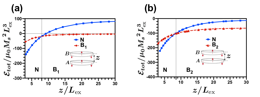
Figure 9: Normalized total energy as a function of the vertical distance $z$ between the two disks for (a) $K_{u}=143$ kJ/m³ and (b) $K_{u}=150$ kJ/m³, at $x=0$. The symbols represent the different configurations: $B_{1}$ (dots), $B_{2}$ (triangles), and $N$ (squares).

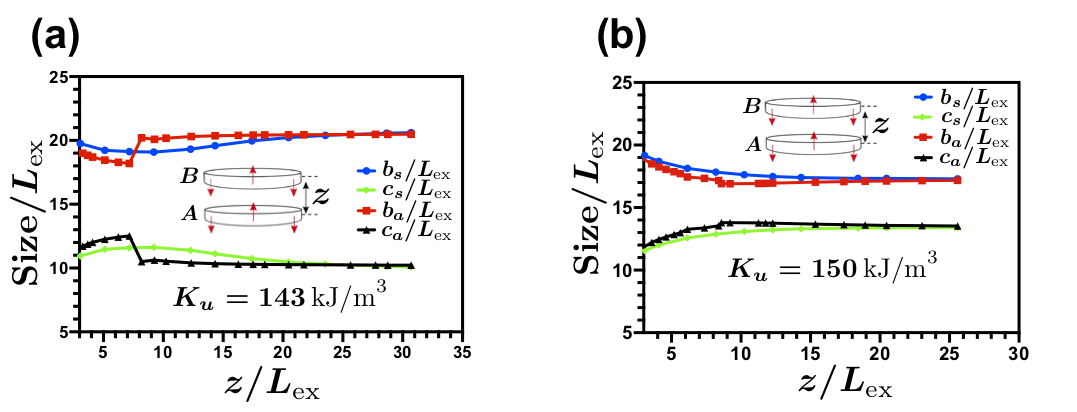
Figure 10: The core, $b$, and the edge-width, $c$, sizes of two disks with the parallel bubble skyrmion configurations as a function of $z$ at $h=10$ nm $/L_{\text{ex}}\approx 1.02$ and $r=300$ nm$/L_{\text{ex}}\approx 30.67$. $(a)$ The anisotropy is $K_{u}=143$ kJ/m³. (b)The anisotropy is $K_{u}=150$ kJ/m³.

Figure 10 shows the variation of the magnetic parameters $b$ and $c$ of the two skyrmions as a function of $z$. We consider $K_{u}=143$ kJ/m³ and $K_{u}=150$ kJ/m³ for Fig. 10(a) and Fig. 10(b), respectively. By decreasing the distance between the disks, the cores sizes of the skyrmions increase for $z<7.16L_{\text{ex}}$ for $K_{a}=143$ kJ/m³ and all the study range of $z$ for $K_{a}=150$ kJ/m³. However the edge-width sizes of the skyrmions decrease for $z<7.16L_{\text{ex}}$ for $K_{a}=143$ kJ/m³ and all the study range of $z$ for $K_{a}=150$ kJ/m³. To understand this behavior for these zones, we observe the magnetic charges (related to the normal component of $\vec{M}$) on the surfaces of the magnetic disks. We will call $B$ the upper disk and $A$ the lower disk. Both disks have a parallel magnetic configuration. We consider that they are very close together so that $z\approx H$. Disk $A$ has a magnetic charge $-q$ on the top surface of the edge-width while disk $B$ has a magnetic charge $q$ on the bottom surface of the edge-width. This configuration is stable because the interaction between the disks reduces the magnetic energy causing that the core sizes of the skyrmions increase. For this reason the core sizes of the skyrmions increase when $z$ decreases because opposite magnetic charges are attracted. The edge-width sizes decrease because for close distance the condition $b+c=R$ occurs. From Fig. 10(a) or $K_{a}=143$ kJ/m³, we observe that the analytical model for $z>7.16L_{\text{ex}}$ does not reproduce the behavior of the core and edge width sizes. The reason is that the magnetic profile for $K_{a}=143$ kJ/m³ is more complex. Figure (11) illustrates a comparison between the analytical profile of $m_{z}$ and the micromagnetic simulations for $K_{u}=143$ kJ/m³. We observe that the magnetic profiles of $m_{z}$ obtained by micromagnetic simulations, for the $B_{1}$ configuration, are different from the analytical profile that we consider, i.e., there is a continuous transition from the Néel configuration (with $m_{\phi}=0$ and $m_{\rho}\neq 0$) to the Bloch configuration (with $m_{\phi}\neq 0$ and $m_{\rho}=0$).

To finalize, we did not consider the case of antiparallel configuration when one disk is over the other. The reason is that we did not observe this configuration in the micromagnetic simulation performed by OOMMF when the disks have a strongly magnetostatic interaction.

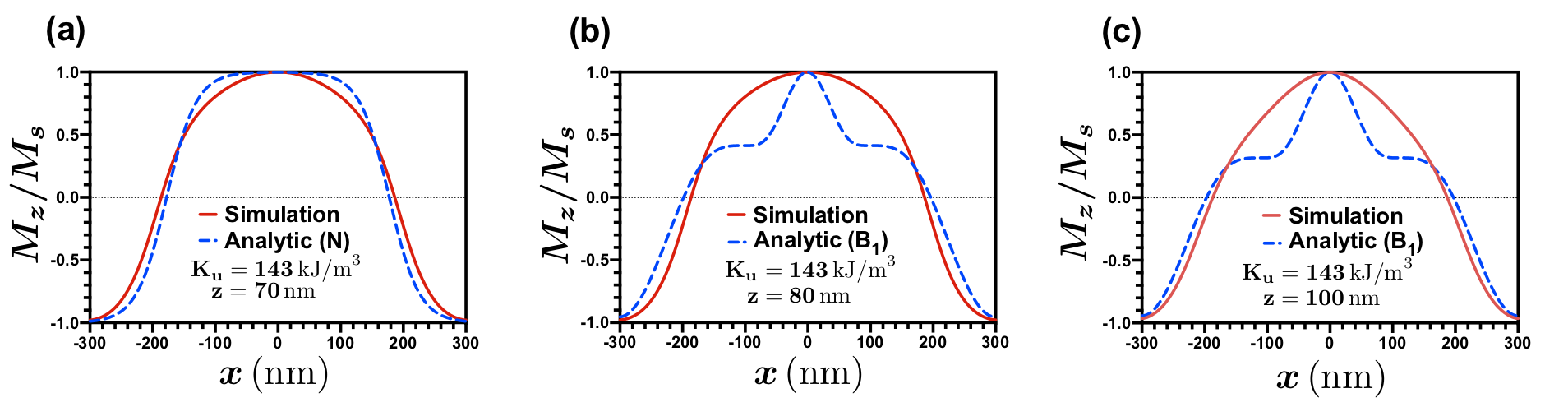
Figure 11: Component $z$ of the normalized magnetization at different vertical distance $z$ of two disks with the parallel bubble skyrmion configuration. The top row is for $K_{u}=143$ kJ/m³ and the bottom row is for $K_{u}=150$ kJ/m³. Each disk has $h=10$ nm $/L_{\text{ex}}\approx 1.02$ and $r=300$ nm$/L_{\text{ex}}\approx 30.67$.

Conclusions

In summary, by means of an analytic model and numerical calculations, we have studied the dependence of the core and edge-width sizes for two magnetic disks, that have a bubble skyrmion configuration, that are interacting by the magnetostatic interaction. By using different ansatz for the magnetic profile of a bubble skyrmion, it was possible to obtain an expression for the magnetostatic interaction energy between the two disks. We observed that the magnetic parameters that describe a skyrmion vary in different ways depending on the location of the disks. When the disks are separated by a horizontal distance, the configuration with minimum energy corresponds to the skyrmions that have an anti-parallel orientation. Results show that if the horizontal distance decreases, the core sizes of the skyrmions decrease and the edge-width sizes of the skyrmions increase. These results can be explained by the magnetic interactions between the magnetostatic fields created by the magnetizations of the cores and the edge-widths of the skyrmions. When one disk is over the other, the configuration with minimum energy corresponds to skyrmions that have a parallel orientation. As the vertical distance decreases, we observe that the bubble skyrmion configuration with a Néel-like skyrmion configuration is stabilized by the magnetostatic interaction, without the Dzyaloshinskii-Moriya interaction, i.e., there is a transition from the Bloch-like to the Néel-like configuration. Thus, these results can be used in the fabrication of future magnetic devices in which two or more bubble-type skyrmions are present.

Author contributions statement

M. A. C., D. M-A., and S. A. carried out numerical analysis and prepared the the figures. D. M-A., J. A. V., and S. A. contributed to write the manuscript. All authors reviewed the manuscript.

Additional information

Competing interests: The authors declare no competing interests.

References

- [1] Fert, A., Cros, V. & Sampaio, J. Skyrmions on the track. Nat. Nanotech. 8, 152–156 (2013).
- [2] Zhang, X., Zhou, Y., Ezawa, M., Zhao, G. P. & Zhao, W. Magnetic skyrmion transistor: skyrmion motion in a voltage-gated nanotrack. Sci. Rep. 5, 11369 (2015).
- [3] Iwasaki, J., Mochizuki, M. & Nagaosa, N. Current-induced skyrmion dynamics in constricted geometries. Nat. Nanotech. 8, 742–747 (2013).
- [4] Sampaio, J., Cros, V., Rohart, S., Thiaville, A. & Fert, A. Nucleation, stability and current-induced motion of isolated magnetic skyrmions in nanostructures. Nat. Nanotech. 8, 839–844 (2013).
- [5] Zhang, X., Ezawa, M. & Zhou, Y. Magnetic skyrmion logic gates: conversion, duplication and merging of skyrmions. Sci. Rep. 5, 9400 (2015).
- [6] Zhang, X. et al. Skyrmion-skyrmion and skyrmion-edge repulsions in skyrmion-based racetrack memory. Sci. Rep. 5, 7643 (2015).
- [7] Rohart, S. & Thiaville, A. Skyrmion confinement in ultrathin film nanostructures in the presence of dzyaloshinskii-moriya interaction. Phys. Rev. B 88, 184422 (2013).
- [8] Guslienko, K. Y. Skyrmion state stability in magnetic nanodots with perpendicular anisotropy. IEEE Magn. Lett. 6, 1–4 (2015).
- [9] Montoya, S. A. et al. Tailoring magnetic energies to form dipole skyrmions and skyrmion lattices. Phys. Rev. B 95, 024415 (2017).
- [10] Montoya, S. A. et al. Resonant properties of dipole skyrmions in amorphous fe/gd multilayers. Phys. Rev. B 95, 224405 (2017).
- [11] Wang, C., Xiao, D., Chen, X., Zhou, Y. & Liu, Y. Manipulating and trapping skyrmions by magnetic field gradients. New J. Phys. 19, 083008 (2017).
- [12] Castro, M. A. & Allende, S. Skyrmion core size dependence as a function of the perpendicular anisotropy and radius in magnetic nanodots. J. Magn. Magn. Mater. 417, 344–348 (2016).
- [13] Büttner, F. et al. Dynamics and inertia of skyrmionic spin structures. Nat. Phys. 11, 225–228 (2015).
- [14] Mochizuki, M. Controlled creation of nanometric skyrmions using external magnetic fields. Appl. Phys. Lett. 111, 092403 (2017).
- [15] Sun, L. et al. Creating an artificial two-dimensional skyrmion crystal by nanopatterning. Phys. Rev. Lett. 110, 167201 (2013).
- [16] Gilbert, D. A. et al. Realization of ground-state artificial skyrmion lattices at room temperature. Nat. Commun. 6, 8462 (2015).
- [17] Müller, J. Magnetic skyrmions on a two-lane racetrack. New J. Phys. 19, 025002 (2017).
- [18] Ding, J., Yang, X. & Zhu, T. Manipulating current induced motion of magnetic skyrmions in the magnetic nanotrack. J. Phys. D: Appl. Phys. 48, 115004 (2015).
- [19] Sun, L. et al. Creating an artificial two-dimensional skyrmion crystal by nanopatterning. Phys. Rev. Lett. 110, 167201 (2013).
- [20] Donahue, M. J. & Porter, D. G. Ommf users guide, version 1.0. Interagency Report NISTIR 6376, (1999).
- [21] Novais, E. R. P. et al. Properties of magnetic nanodots with perpendicular anisotropy. J. Appl. Phys. 110, 053917 (2011).
- [22] Aharoni, A. Introduction to the Theory of Ferromagnetism. International Series of Monographs on Physics (Oxford University Press, 2000).
- [23] Landeros, P. et al. Scaling relations for magnetic nanoparticles. Phys. Rev. B 71, 094435 (2005).
- [24] Altbir, D., Escrig, J., Landeros, P., Amaral, F. S. & Bahiana, M. Vortex core size in interacting cylindrical nanodot arrays. Nanotechnology 18, 485707 (2007).
- [25] Porrati, F. & Huth, M. Micromagnetic structure and vortex core reversal in arrays of iron nano-cylinders. J. Magn. Magn. Mater. 290-291, 145–148 (2005).
- [26] Tanigaki, T. et al. Three-dimensional observation of magnetic vortex cores in stacked ferromagnetic discs. Nano Lett. 15, 1309–1314 (2015).
- [27] Reyes, D., Biziere, N., Warot-Fonrose, B., Wade, T. & Gatel, C. Magnetic configurations in co/cu multilayered nanowires: Evidence of structural and magnetic interplay. Nano Lett. 16, 1230–1236 (2016).
Acknowledgements
We acknowledge financial support in Chile from FONDECYT 1161018, Financiamiento Basal para Centros Científicos y Tecnológicos de Excelencia FB 0807, and AFOSR Neuromorphics Inspired Science FA9550-18-1-0438. M. A. C acknowledges Conicyt-PCHA/Doctorado Nacional/2017-21171016. D. M.-A. acknowledges financial support in Chile from CONICYT, Postdoctorado FONDECYT 2018, folio 3180416.