The AGN Ionization Cones of NGC 5728 : II - Kinematics

Abstract

We explore the gas morphology and excitation mechanisms of the ionization cones of the Type II Seyfert galaxy NGC 5728. Kinematics derived from near-IR and optical data from the SINFONI and MUSE IFUs on the VLT reveal AGN-driven outflows powered by a super-massive black hole (SMBH) of mass $3.4\times 10^{7}$ M_⊙, bolometric luminosity of $1.46\times 10^{44}$ erg s^-1, Eddington ratio $3.3\times 10^{-2}$ and an accretion rate of $2.7~{}\times 10^{-2}$ M_⊙ yr^-1. The symmetric bicone outflows show rapid acceleration to $\pm 250$ km s^-1 at $\sim 250$ pc, then decelerating to $\sim 130$ km s^-1 at 500 pc from the AGN, with an estimated mass outflow rate of 38 M_⊙ yr^-1; the mass ratio of outflows to accretion is 1415. The kinetic power is $1.5\times 10^{42}$ erg s^-1, 1% of the bolometric luminosity. Over the AGN active lifetime of $\sim$10⁷ years, $1.6\times 10^{8}~{}\rm M_{\odot}$ of gas can become gravitationally unbound from the galaxy, a large proportion of the gas mass available for star formation in the nuclear region. The bicone internal opening angle (50°.2) and the inclination to the LOS (47°.6) were determined from [Fe II] line profiles; the outflow axis is nearly parallel to the plane of the galaxy. This geometry supports the Unified Model of AGN, as these angles preclude seeing the accretion disk, which is obscured by the dusty torus.

1 Introduction

This is the second of two papers studying the narrow-line region (NLR) of the Seyfert 2 galaxy NGC 5728 using data acquired from the SINFONI and MUSE Integral Field Unit (IFU) spectroscopic instruments on ESO’s VLT telescope. This galaxy has a complex nuclear structure, with a spectacular ionization cones emanating from the hidden active galactic nucleus (AGN), an inner star forming ring and spiraling central dust lanes (Gorkom, 1982; Schommer et al., 1988; Wilson et al., 1993; Mediavilla & Arribas, 1995; Capetti et al., 1996; Rodríguez-Ardila et al., 2004, 2005; Dopita et al., 2015). Urry & Padovani (1995), in the seminal review paper on AGN unification, cited NGC 5728 as the paradigm of a Type 2 AGN with ionization cones; these are predicted by the Unified Model of AGN, as radiation from the accretion disk is collimated by the surrounding dusty torus to impinge on the ISM, exciting the gas by photo-ionization. This object is a prime target for investigation, particularly using observations in the near infrared, allowing penetration of obscuring dust.

In our previous paper (Durré & Mould, 2018, hereafter ‘Paper I’), we explored the near infrared (NIR) flux distributions and line ratios of [Fe II], H₂, [Si VI] and hydrogen recombination emission lines, plus the optical H $\alpha$, H $\beta$, [O III], [S II] and [N II] emission lines, to characterize gas excitation mechanisms, gas masses in the nuclear region and extinction around the AGN. In this paper, we will use these data to examine the kinematics of the cones, determining mass outflow rates and power and relate these to the AGN bolometric luminosity and the amount of gas that can be expelled during the AGN activity cycle. We will also determine the stellar kinematics and relate them to the gas kinematics. The super-massive black hole (SMBH) mass will be determined by several methods and the Eddington ratio deduced.

Our conclusions from Paper I were as follows:

• Dust lanes and spiraling filaments feed the nucleus, as revealed by the HST structure maps.

• A star-forming ring with a stellar age of 7.4 – 8.4 Myr outlines a nuclear bulge and bar.

• A one-sided radio jet, impacting on the inter-stellar medium (ISM) at about 200 pc from the nucleus, is combined with radio emission from the supernova (SN) remnants in the SF ring.

• Ionized gas in a bi-cone, traced by by emission lines of H I, [Fe II] and [Si VI], extends off the edges of the observed field. MUSE [O III] data shows that the full extent of the outflows is over 2.5 kpc from the nucleus. The cones are somewhat asymmetric and show evidence of changes in flow rates, plus impact on the ISM, combined with obscuration.

• The AGN and BLR is hidden by a dust bar of size $64\times 28$ pc, with up to 19 magnitudes of visual extinction, with an estimated dust temperature at the nuclear position of $\sim 870$ K. Extinction maps derived from both hydrogen recombination and [Fe II] emission lines show similar structures, with some indication that [Fe II]-derived extinction does not probe the full depth of the ionization cones. There is evidence for dust being sublimated in the ionization cones, reducing the extinction. This is supported by extinction measures derived from MUSE H $\alpha$/H $\beta$ emission, which show much decreased absorption in the ionization cones.

• An extended coronal-line region is traced by [Si VI], out to $\sim 300$ pc from the nucleus. This is excited by direct photo-ionization from the AGN, plus shocks from the high-velocity gas. Higher-ionization species ([Ca VIII] and [S IX]) are closely confined around the AGN.

• NIR line-ratio active galaxy diagnostics show mostly AGN-type activity, with small regions of LINER and TO modes at the peripheries of the cones and where the dusty torus obscures the direct photo-ionization from the BH. MUSE optical diagnostics (BPT diagrams) show a clean star-formation/AGN mixing sequence.

• The H₂ gas is spatially independent of the cones, concentrated in an equatorial disk in the star-forming ring, but also showing entrainment along the sides of the bicone. The warm H₂ has a mass of 960 M_⊙, with an estimated $6\times 10^{8}~{}\rm M_{\odot}$ of cold H₂ in the field of view. Line-ratio diagnostics indicate that the gas is excited by thermal processes (shocks and radiative heating of gas masses) to temperatures in the range 1400– 2100 K, with an increased fluorescent excitation towards the SF ring.

• With 100 pc of the nucleus, the ionized gas mass (derived from the Br $\gamma$ emission) is $8\times 10^{5}~{}\rm M_{\odot}$ and the cold gas mass (from extinction calculations) is $4.9\times 10^{6}~{}\rm M_{\odot}$; however this could be underestimated due to dust sublimation in the cones.

2 Observations, Data Reduction and Calibration

The data acquisition, reduction and calibration procedure was described in detail in Paper I. 3D data cubes were produced from the SINFONI and MUSE observations, as laid out in Table 1. Subsequent cube manipulation and computation is done using the the cube data viewer and analysis application QFitsView (Ott, 2012), which incorporates the DPUSER language. In this paper, we use the standard cosmology of H${}_{0}=73$ km s^-1Mpc^-1, $\Omega_{Matter}=0.27$ and $\Omega_{Vacuum}=0.73$. All images are oriented so that North is up, East is left, as indicated in Figure 1.

Table 1: 3D Data Cubes from IFU observations

Instrument	Filter	FOV (″)	Plate Scale (″)
	$\lambda$ range (nm)	FOV (pc)	R ($\Delta\lambda/\lambda$)
SINFONI	J	8	0.25
	1095–1402	1600	2400
SINFONI	H+K	3.8	0.1
	1452–2457	760	1560
MUSE	V	68.2	0.2
	475–935	13640	1800

3 Results

3.1 Deriving Kinematic Parameters

We use the QFitsView velmap function; this fits a Gaussian curve for every spaxel at the estimated central wavelength and full width half maximum (FWHM). This generates maps of the best fit continuum level (C), height (H), central wavelength ($\lambda$) and FWHM. These are readily converted to the dispersion ($\sigma$), the flux (F) and the emission equivalent width (EW).

Map values are accepted or rejected based on ranges on each of the derived parameters produced by the procedure, based on visual inspection of the fluxes and kinematic structures i.e. the derived values of continuum, line flux, LOS velocity or dispersion have to be within certain values. Single pixels may be rejected because of large excursions from their neighbors; the source of anomalous values is usually noise spikes in the data or low flux values, causing poor model fits. Rejected pixels are then interpolated over from neighbors or masked out, as appropriate.

3.2 Stellar Kinematics

The stellar kinematics help to disentangle the complex nuclear structure and also give an estimate for the SMBH mass. They are derived from the Si I line in the H-band at 1589.2 nm using the velmap procedure from QFitsView. This procedure is designed for emission lines; the spectrum was inverted to turn an absorption line into a peak. The resulting (cleaned) velocity and dispersion map is presented in Fig. 1. This shows a simple rotation around the east-west axis; the average dispersion in the central 0″.5 radius is $230\pm 26$ km s^-1 and the systemic velocity is $2984\pm 55$km s^-1. Combined with the wavelength calibration and the barycentric velocity corrections (derived above), our systemic velocity is 2937 km s^-1, compared to the H I 21 cm velocity of 2786 km s^-1 (Roth et al., 1991) and the H $\alpha$-derived velocity of 2804 km s^-1 (Catinella et al., 2005). The difference can be ascribed to the H I measuring the velocity of the whole galaxy and the H $\alpha$ velocity including gas with a non-zero peculiar velocity.

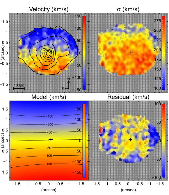
Figure 1: Top row : Stellar LOS velocity and dispersion from the Si I absorption line (1589 nm). Contours are the H-band normalized flux, from 30 to 90% of maximum, in steps of 10%. Velocity and dispersion values in km s^-1. Bottom row : Plummer model fit and residual. This shows the ordered, tumbling rotation of the circumnuclear stellar structure, mis-aligned to the main galactic plane rotation axis by $\sim 60\arcdeg$.

The stellar velocity field derived from the Si I line is modeled using the Plummer potential, (Plummer, 1911) (see e.g. Riffel & Storchi-Bergmann, 2011).

$$V_{LOS}=V_{Sys}+\dfrac{\sqrt{\dfrac{R^{2}GM}{(R^{2}+A^{2})^{3/2}}}\left[\sin(i)\cos(\Psi-\Psi_{0})\right]}{\left[\cos^{2}(\Psi-\Psi_{0})+\dfrac{\sin^{2}(\Psi-\Psi_{0})}{\cos^{2}(i)}^{3/2}\right]}$$ (1)

where $V_{LOS}$ and $V_{Sys}$ are the observed line of sight and systemic velocities, R is the projected distance from the nucleus, $\Psi$ is the position angle, $\Psi_{0}$ is position angle of the line of nodes, G is the gravitational constant, A is the scale length, i is the disk inclination (i=0 for face-on) and M is the enclosed mass. Including the location of the kinematic center, this equation has 6 free parameters. The kinematic center and line of nodes can be well-constrained from the observations. Standard techniques (e.g. Levenberg–-Marquardt least-squares fitting algorithm) are used to solve for the parameters.

The model was fitted with the generalized reduced gradient algorithm (‘GRG Nonlinear’) implemented in the MS-Excel add-on Solver. We centered the kinematics on the AGN location. The model and residual results are also shown in Fig. 1. The axis PA is 1°.4 (i.e. the rotational equator is nearly edge-on to the LOS), with negligible inclination (-0°.39), i.e. the ring is essentially face-on, and a scale length of $\sim 395$ pc (i.e. off the edge of the field). A slice through the measured velocity field along the axis produces a velocity gradient of 205 km s^-1 over 140 pc, which implies an enclosed mass of $\sim 3.5\times 10^{8}~{}\rm M_{\odot}$, assuming simple Keplerian rotation.

The kinematics of the inner ring and bar match (to first order) those of the molecular hydrogen (see Section 3.3.2); however, if this ring of star formation is a disk structure, then it appears not to be rotating about its normal axis, which would be almost along the LOS. Instead the Plummer model shows that the rotation axis is almost east-west and the ring is ‘tumbling’, mis-aligned to the main galactic plane rotation axis by $\sim 60\arcdeg$.

A large-scale plot of the stellar kinematics was obtained using the MUSE data cube, using the 8544 Å Ca II triplet absorption feature (using the velmap procedure in QFitsView). The derived velocity and dispersion is shown in Fig. 2. The ‘Weighted Voronoi Tessellation’ (WVT) (Cappellari & Copin, 2003) was used to increase the S/N for pixels with low flux; we use the voronoi procedure in QfitsView. This aggregates spatial pixels in a region to achieve a common S/N, in this case set to 60. This needs both signal and noise maps, which were, respectively, the white-light image and from the square-root of the average variance statistics from the MUSE data. Within the central 1″, the velocity dispersion is $\sigma_{*}=178.7\pm 10.1$ km s^-1, again compatible with the values derived above for the CO band-heads.

The rotational axis is skewed from the outer regions to the inner, but the change is not discontinuous; this is different from the long-slit results from Prada & Gutiérrez (1999), who found that the core is counter-rotating with respect to the main galaxy. The dispersion values show a suppression at the SF ring and then an inwards rise; the inner reduction was also seen by Emsellem et al. (2001) using the ISAAC spectrograph of the VLT. The skewed velocity field and central dispersion drop are characteristic of inner bars that are rotating faster than the primary bar; at the inner Lindblad resonance (ILR) of the primary bar (which is presumed to be the location of the SF ring), the gas accumulates (driven there by the gravity torque of the bar), and then forms stars. The dispersion of the young stars reflects the gas dispersion, and is lower than that of the old stars. The inner rise is then due the greater prevalence of old bulge stars, plus the presence of the SMBH. (F. Combes, B. Ciambur, pers. comm.).

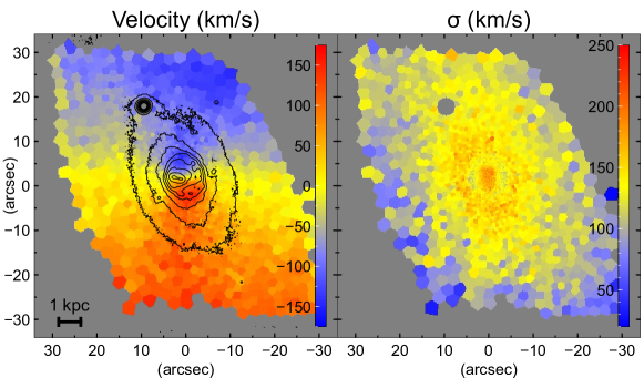
Figure 2: Top row : Stellar LOS velocity and dispersion from the Ca II absorption line (from MUSE data). Contours are the V-band surface brightness magnitude, in steps of 0.5 mag from 17.5 to 21 mag deg^-2. Velocity and dispersion values in km s^-1. Values have been smoothed in the inner $28\arcsec\times 28\arcsec$. Note that the kinematics and photometry are aligned, and the stellar dispersion is suppressed in the SF ring. The feature in the NE quadrant in the photometry is a foreground star.

3.3 Gaseous Kinematics

3.3.1 Line-of-sight Velocity and Dispersion

The kinematics of gas around the nucleus diagnose outflow, inflow and rotational structures in the nuclear region; combined with the emission-line flux, we can compute the energetics of this gas. Different species have different kinematics structures, e.g. outflows are prominent in hydrogen recombination and other ionized emission lines, whereas molecular hydrogen tends to be in a rotating gas disk around the center.

In Figs. 3 and 4 we present the line-of-sight velocity and dispersion for the main emission lines in the J and H+K band. We use the kinematics of these lines to delineate outflows, rotations and (possible) feeding flows. We set the velocity zero-point at the location of the AGN; see section 3.5 of Paper I.

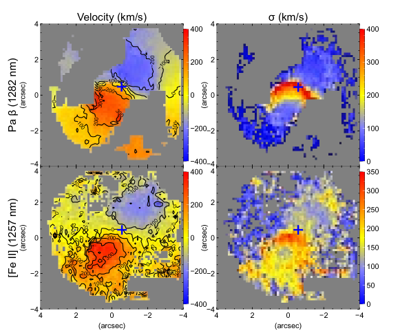
Figure 3: Kinematics for Pa $\beta$ and [Fe II] (1257 nm). Flux units 10^-16 erg cm^-2 s^-1, EW units in nm. Both species show the strong bi-polar flow in velocity, with the nuclear dispersion being much higher for hydrogen recombination than [Fe II]. The zero velocity point is set at the AGN location. White pixels are where the emission line was too weak to derive the kinematics.

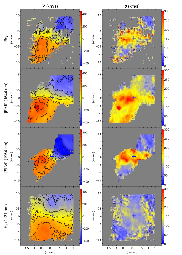
Figure 4: As for Fig. 3 for Br $\gamma$, H₂ (2121 nm), [Fe II] (1644 nm) and [Si VI].

From the Pa $\beta$ kinematics, the velocity field reaches a maximum of about -250 km s^-1 at 1″.1 NW ($\sim 220$ pc projected distance) and 270 km s^-1 at 1″.4 ($\sim 280$ pc) SE of the nucleus, then decelerates to -150/110 km s^-1 at double the respective distances from the nucleus. This profile suggests gas accelerated away from the AGN by radiation pressure, then decelerating as it interacts with the ISM and the radiation pressure drops off with increasing distance from the source. High absolute velocity values in the northern and southern parts of the field are due to the star-forming ring rotation, aligned with the stellar kinematics along a PA of $\sim 10\arcdeg$ (see Section 3.2). The [Fe II] velocity field shows a similar pattern to the Pa $\beta$ field, however the peak velocity is further from the AGN.

The Br $\gamma$, [Fe II] 1644 nm and [Si VI] velocity and dispersion maps show very similar structure, as is also the case for the flux and EW. Again, the H₂ kinematics do not align with the other species (see Section 3.3.2). For [Fe II] 1257 nm, the higher dispersion is more extended; around the SE cone, the higher values outline the cone, supporting an emission mechanism of a shock boundary. The Br $\gamma$, [Fe II] 1644 nm and [Si VI] dispersion plots show the same structure at higher spatial resolution.

We present histograms of the velocity and dispersion values in Figs. 5. The H II and [Si VI] velocity histograms show the characteristic double peak of outflows or rotation, which is also shown in the [Fe II] 1644 nm line. The negative [Si VI] velocities are somewhat higher than the Br $\gamma$ velocity; for the receding velocities, [Fe II] has higher values than Br $\gamma$ and [Si VI], with a modal value of $\sim 200$ km s^-1; there is a small group of pixels with a velocity of $\sim$-300 – -400 km s^-1. The [Fe II] 1257 nm line shows a stronger concentration around zero velocity; this is because the J-band map takes in a larger area than the H+K-band map, where there is a large partially-ionized volume of gas which is not in the outflow and therefore has a lower velocity.

The [Fe II] dispersion distribution is more extended than Br $\gamma$, as seen both in the maps and histograms. As it has a lower ionization potential than H I, it is only found in partially ionized media. In this case, it is on the edge of the cones, which will broaden the line from the LOS components of the velocity, and by turbulent entrainment at the cone boundaries. This is clearly seen in the map of the [Fe II] 1257 nm dispersion, showing a ring of higher dispersion around the SE outflow. The [Si VI] dispersion values seem to be somewhat bi-modal, with high values more or less coincident with the high values for [Fe II] and lower values elsewhere; this may reflect the production mechanisms, i.e. photo-ionization where directly illuminated by the accretion disk, with low dispersion, and shocks (high dispersion) on the outflow boundaries.

The high dispersion values observed for Pa $\beta$ perpendicular to the cones across the nucleus can be attributed to the beam-smearing, causing the LOS to intersect both the approaching and receding outflows and broadening the line artificially; the Seyfert classification for this object was altered from Sy 1.9 (i.e. broad H $\alpha$ emission lines present) to Sy 2 (no broad lines present) (Shimizu et al., 2018).

We plot the velocity and dispersion for the H+K-band lines in a slice along the bicone centerline in Fig. 6. The velocity profile is virtually identical for all species, except for a region in the NW outflow (approaching) with a higher velocity for [Si VI].

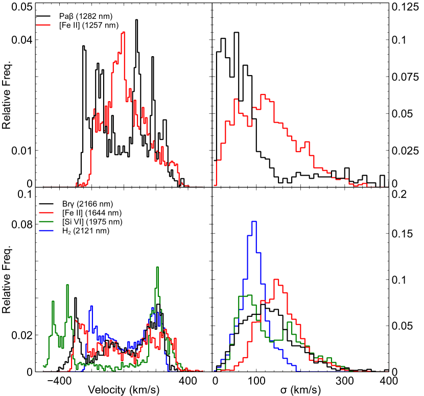
Figure 5: Top panels: Velocity (left) and dispersion (right) distribution histograms for Pa $\beta$ and [Fe II] (1257 nm). The higher [Fe II] dispersion is from line-broadening by LOS components of the outflow velocity and turbulent entrainment. Bottom panels: Velocity (left) and dispersion (right) distribution histograms for Br $\gamma$, H₂ (2121 nm), [Fe II] (1644 nm) and [Si VI]. The H₂ is kinematically colder than the other species.

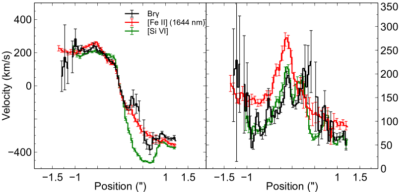
Figure 6: LOS velocity and dispersion along the bicone centerline, centered on the AGN location, showing the steep gradient near the AGN and the asymptotic flattening further out.

For comparison, the [O III] and H $\beta$ flux and kinematic maps from the MUSE archival data (seeing-limited at $\sim 0\arcsec.7$) are also presented here. These were produced in the same manner as the SINFONI kinematic maps. Figs. 7 shows the inner $9\times 9$ kpc. The [O III] delineates the bicone, whereas the H $\beta$ also includes the SF ring; the distortion in the LOS velocity field for H $\beta$ from the combination of the SF ring and the outflows is clearly seen. Kinematic values are the same as the SINFONI observations; however the high values of the LOS dispersion aligned NE/SW across the nucleus are due to the overlapped outflow edges measured with limited (0″.2) plate scale resolution.

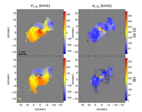
Figure 7: [O III] and H $\beta$ kinematics from MUSE. Hydrogen recombination emission delineates both the outflow and the SF ring, whereas [O III] is only excited in the outflow.

3.3.2 Molecular Hydrogen Kinematics

Molecular hydrogen (H₂) is the direct source material for star formation; its location and kinematics help diagnose SF processes and AGN/SF linkages. Most H₂ structures in Seyfert galaxies are in rotating disks (Diniz et al., 2015). As we illustrated in Fig. 4, the H₂ velocity structure is aligned with a PA of $\sim 350\arcdeg$ while the bicone has a PA of $\sim 315\arcdeg$; the ordered PV diagram also suggests simple rotation (see Section 3.3.4). Interestingly, this orientation is not in the plane either of the whole galaxy, or the inner structure (either disk or bar), unlike other examples (see e.g. NGC 4151, Storchi-Bergmann et al., 2010).

The H₂ LOS velocities and dispersions are kinematically colder than for [Fe II], Br $\gamma$ and [Si VI] (Fig. 5), reaching a maximum velocity of $\sim\pm$250 km s^-1 vs. $\sim\pm$300–400 km s^-1 for the ionic species, and a median (maximum) dispersion of $\sim$95 km s^-1 (200 km s^-1) vs. $\sim$130 km s^-1 (350 km s^-1) for Br $\gamma$. These trace different astrophysics; a cold molecular gas ring with kinematically associated star-formation vs. AGN-driven outflows.

We fitted a Plummer potential model to the H₂ velocity field, using the method described in Section 3.2. Initially, the five parameters (kinematic center [$X_{0},Y_{0}$], line of nodes, inclination and scale length) were left reasonably unconstrained. The fitted alignment was 347°, with the kinematic center located 0″.09 from the AGN position (equivalent to 17 pc projected distance). Fig. 9 shows the result. The model rotation axis is aligned at PA = 77–257° (polar alignment 13–193°), with a very low inclination, i.e. almost edge-on. The scale length is approximately 0″.9, which corresponds to 180 pc.

We also fitted the model where we constrained the kinematic center to the position of the AGN (assuming that the SMBH is the center of rotation). The polar alignment was also constrained to align with the main NS ridge of the equivalent width plot (the line of nodes constrained to between 260–265°). The results are shown in Fig. 9. The scale length and inclination are very similar to the unconstrained fit. Both residuals plots show a region to the east to SE of the nucleus of the gas disk which shows negative residual velocities; these are hypothesized to be gas entrained on the edges of the bicone. This is seen in the pronounced clockwise ‘twist’ of both the flux and velocity contours from the center. This is supported by the CO(1-0) radio emission morphology (which traces the extended molecular hydrogen), as reported by Combes & Leon (2002) from observations using the IRAM-30 m telescope.

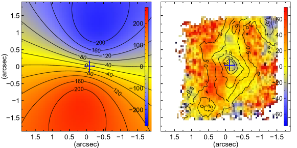
Figure 8: Plummer model for H₂ velocity field with unconstrained parameters. Left panel: H₂ velocity field. Middle panel: Best fit Plummer model. Right panel: Residual velocity with H₂ equivalent width contours overplotted (in nm). All velocities shown in km s^-1.

Figure 9: Plummer model for H₂ velocity field with kinematic center and line of nodes constrained. Left panel: Best fit Plummer model. Right panel: Residual velocity with H₂ equivalent width contours overplotted (in nm). All velocities shown in km s^-1. These show ordered rotation broadly aligned with the stellar kinematics, plus the component of entrainment along the bicone edges.

3.3.3 Channel Maps

We further analyzed the gas kinematics using channel maps and position-velocity diagrams. These are similar, and are both used to reveal kinematic structures that are not visible in the LOS velocity and dispersion plots. The former slice the velocity axis across the LOS, while the latter slice it parallel to the LOS. Figs. 11 to 17 show the channel maps for the spectral lines Pa $\beta$, [Fe II] 1257 nm (both from the J data cube), [Fe II] 1644 nm, Br $\gamma$, H₂ 2121 nm and [Si VI] 1964 nm (from the H+K data cube). The maps were constructed by subtracting the continuum height, derived from the velocity map function velmap, from the data cube. The spectral pixels are velocity binned and smoothed to reduce noise.

The J-band channel maps are at a larger scale, encompassing more of the star-forming ring, as well as the inner bicone, whereas the H+K-band maps show greater detail in the bicone. To separate the bicone and SF ring kinematics, we masked out the central 2″.5 around the AGN location where the bulk of the bicone emission is located (Fig. 14 - the channels are now 30 km s^-1). There is still some impact from the cones (e.g. at the +45 and -135 km s^-1 channels), but the maximum recession velocity is now in the SW quadrant, moving to the NE over the 450 km s^-1 range, rather than the SE–NW direction of the bicone. This velocity range and orientation are compatible with stellar kinematics derived from the Si I absorption line (see Section 3.2 for a discussion of the anomalous kinematics). The star-forming ring has a greater velocity than the cones, because its axis of rotation is perpendicular to our LOS, therefore we measure the full rotation velocity. By contrast, the cones are inclined to our LOS (see Section 4.2.3) and we only measure the component velocity.

The low velocity channels (-112 – +112 km s^-1) show the emission across most of the field; this is due to the common minimum value for the scaling for all channels, to enhance the high-velocity channels. These channels have been replotted in Fig 12 to suppress this noisy background; the -37 km s^-1 show the ‘X’-shaped outline of the bicones.

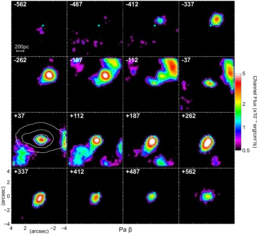
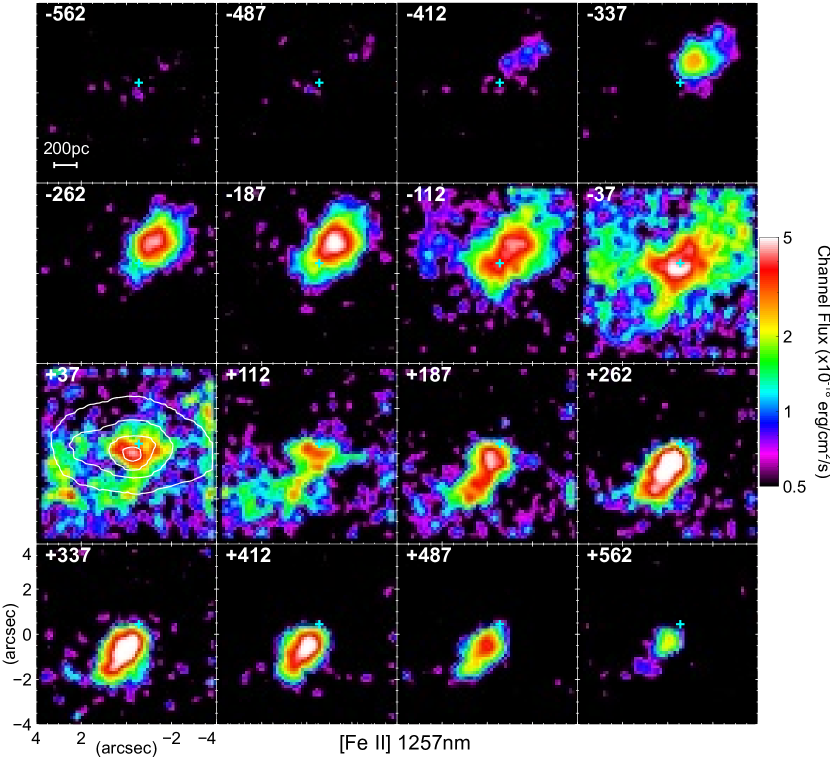
Figure 10: Channel map for Pa $\beta$. Each channel has a width of 75 km s^-1, with the channel central velocity shown in the top left corner of each plot. The cyan cross is the position of the AGN. Color values are fluxes in units of 10^-18 erg cm^-2 s^-1, plotted with log scaling; all channels have the same maximum and minimum values. Positive velocities are receding, negative are approaching. The white contour on the +37 km s^-1 channel is the J-band continuum flux, at levels of 30, 50, 70 and 90% of maximum. Note the 200 pc scale on the -562 km s^-1 channel. The bicone structure is prominent in the NW (approaching) and SE (receding), plus the SF ring component at the peripheries. The outflows, aligned NW-SE are visible, as well as the SF ring emission from -187 to +187 km s^-1.

Figure 11: As for Fig. 11, for [Fe II] 1257 nm.

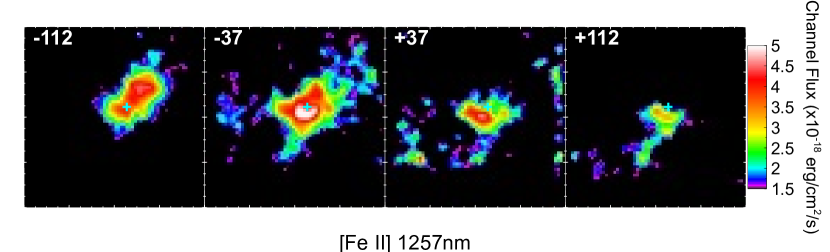
Figure 12: [Fe II] channel maps for low velocity with reduced scale range to enhance structure visibility. The ‘X’-shaped bicone boundaries are visible in the -37 km s^-1 channel.

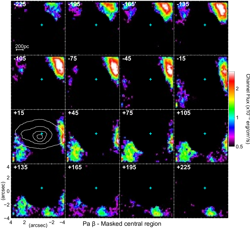
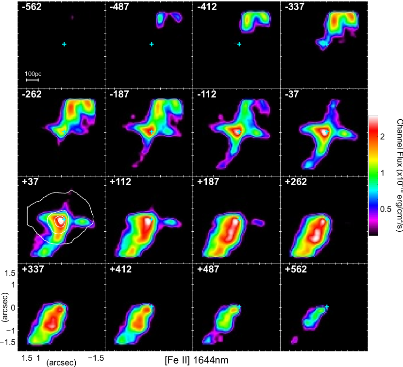
Figure 13: As for Fig. 11, for Pa $\beta$, with the central 2″.5 around the AGN masked out. This enhances the SF ring features. The channel map velocity intervals are now 30 km s^-1.

Figure 14: Channel map for [Fe II] 1644 nm. The white contour on the +37 km s^-1 channel is the H-band continuum flux, at levels of 30, 50, 70 and 90% of maximum. Note the 100 pc scale on the -562 km s^-1 channel. The cross-shaped feature outlining the outflows is especially prominent in the -262 to +37 km s^-1 channels. The [Fe II] emission is from partially ionized and shocked gas, which are the boundaries of the outflows where the accretion disk radiation is weaker and the shear turbulence between the bicone and the ISM is greatest.

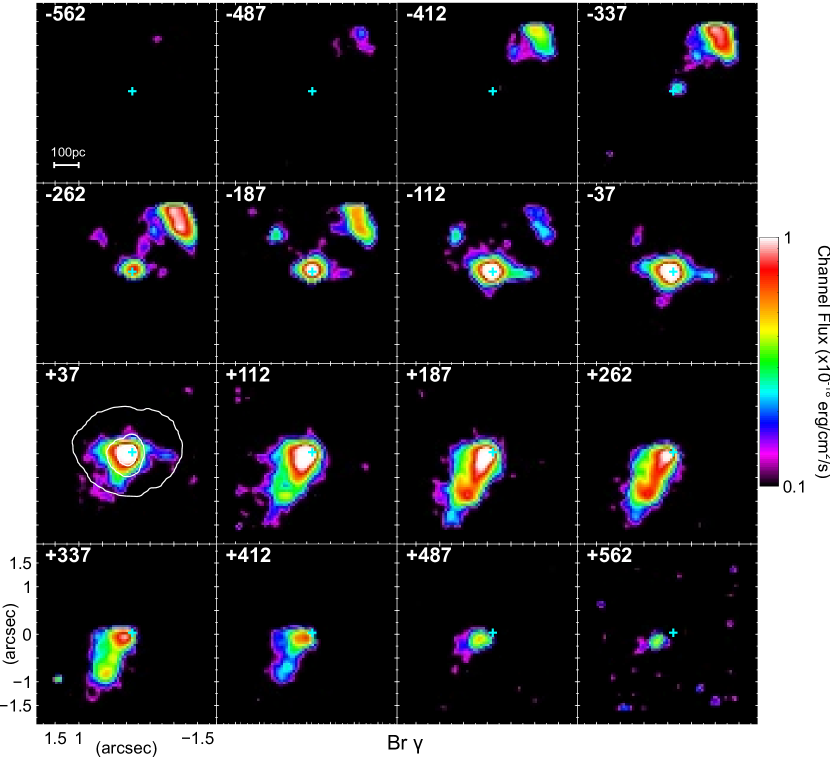
Figure 15: As for Fig. 14, for Br $\gamma$. The white contour on the +37 km s^-1 channel is now the K-band continuum flux, at levels of 30, 50, 70 and 90% of maximum. This is confined to the bicone interior.

Figure 16: As for Fig. 16, for H₂ 2121 nm. The kinematics are oriented more NS, especially in the negative velocity channels, with some entrainment effect by the outflows.

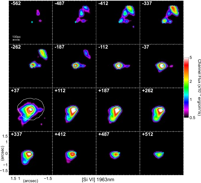
Figure 17: As for Fig. 16, for [Si VI] 1964 nm, strictly confined to the bicone interior closer to the AGN than for Br $\gamma$.

Assuming that the [Fe II] and [Si VI] gas is co-moving with the Br $\gamma$, we can plot the channel flux ratio for those species. These are presented in Figs. 18 and 20. The [Fe II]/Br $\gamma$ channel ratio clearly shows that in the SE cone, the [Fe II] ‘outlines’ the Br $\gamma$ emission, i.e. the flux ratios are higher to the SE, whereas the [Si VI]/Br $\gamma$ channel ratios are higher towards the nucleus. A check whether there is a difference between the outflows is shown in Fig. 20, which plots the average flux ratio for each velocity channel (with the standard deviation as uncertainties). There is a trend in the flux ratios towards the receding (positive) velocities for [Fe II]/Br $\gamma$, and an opposite trend for [Si VI]/Br $\gamma$, but with large uncertainties.

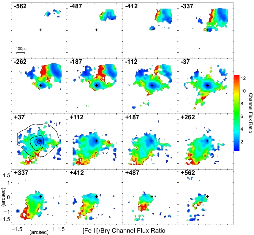
Figure 18: Flux ratio for [Fe II] 1644 nm/Br $\gamma$ for each velocity channel. The color-bar shows the flux ratio, with enhanced values (green and blue) at the peripheries of the cones in the higher velocities, showing enhanced [Fe II] emission in partially ionized and shocked gas.

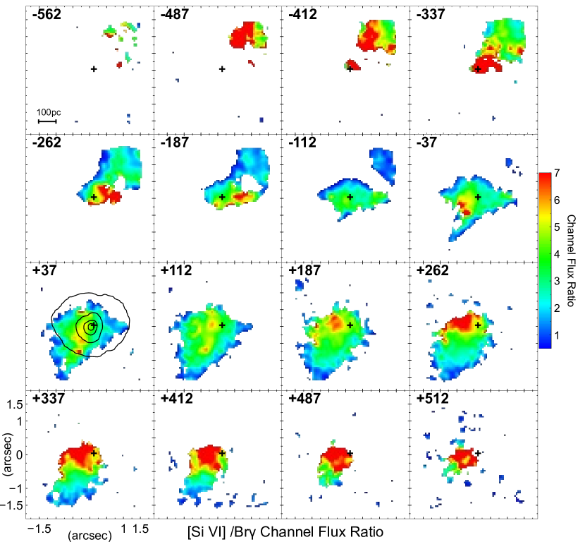
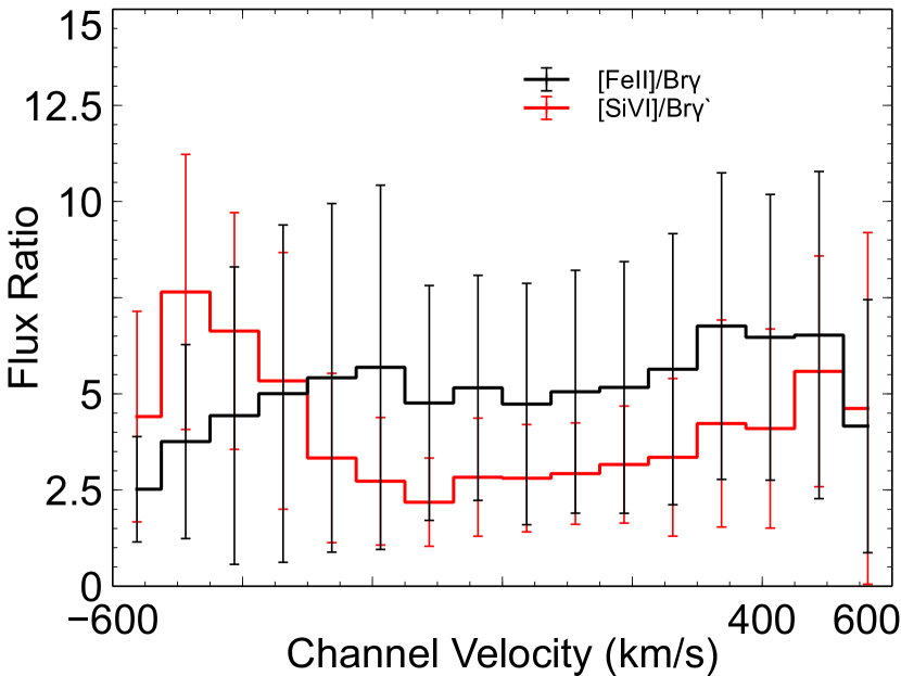
Figure 19: Flux ratio for [Si VI]/Br $\gamma$ for each velocity channel, showing the more central concentration for the [Si VI] from direct photo-ionization from the AGN.

Figure 20: Average flux ratios for each velocity channel, with standard deviation as the uncertainty, showing no significant differences across velocities. This contradicts the model of Murayama & Taniguchi (1998) of a clumpy matter-bound CLR.

3.3.4 Position-Velocity Diagrams

Similarly to the channel maps, the position-velocity (PV) diagram can help to identify features in the cones, like velocity and dispersion anomalies, that are not apparent in the standard kinematic maps. The PV diagram is generated by a ‘pseudo-longslit’ (the longslit function in QFitsView) along the cone or the plane of rotation of the molecular gas. For Br $\gamma$, [Si VI] and [Fe II], the longslit was laid along a PA = 140–320° (NW–SE) centered on the AGN and aligned with the velocity extrema; for H₂ the line was along a PA = 170–350°, along the flux ridge line (presumably the plane of rotation). All slits are 2 pixels wide. The alignment of the longslits is shown in Fig. 21; slit 5 (blue and green) the one aligned with the AGN.

Fig. 23 shows the resulting plots for the central slit; the wavelength (on the X-axis) is converted to a velocity difference from the central pixel, and the Y-axis is the distance along the longslit in arcsec. To enhance the emission line features, the flux values have been divided by the median value along the slit position, otherwise the continuum variations would obscure the details; this is similar to the equivalent width of the emission line. The LOS velocity derived from the velmap procedure is overlaid on the relative flux; these delineate the centerline of the PV diagram at each position.

Figure 21: Longslit alignment, superimposed on [Fe II] flux map; the blue box is the slit for Br $\gamma$, [Si VI] and [Fe II] 1644 nm, the green for H₂. The white boxes are the off-nucleus pseudo-slits through the cones, with the numbers corresponding to the plots in Figs. 23, 24 and 25.

The PV diagrams show a velocity gradient at the nucleus of $\sim$330 (Br $\gamma$), 475 ([Si VI]) and 440 ([Fe II]) km s^-1 per 100 pc, with H₂ having a lower gradient of 175 km s^-1 per 100 pc. The H₂ velocity then levels off to a constant value of approximately $\pm$ 200 km s^-1, presumably as it co-rotates with the stars. In the positive (receding) velocity direction, the Br $\gamma$, [Fe II] and [Si VI] all plateau or slightly decline at roughly the same velocity. However, in the negative (approaching) velocity direction, the Br $\gamma$ does not continue smoothly, presumably because of low flux values introducing uncertainties; the [Fe II] velocity continues rising and the [Si VI] shows a decline from a maximum of $\sim$430 km s^-1 to $\sim$320 km s^-1. It is noted that all three species plateau and the flux brightens at the edge of the field at this velocity; it is hypothesized that the source of this emission is the radio jet interacting with the ISM co-rotating with the inner disk, moving towards us at this velocity, rather than the direct outflow.

Figs. 23 and 24 shows the PV diagrams for [Fe II] and Br $\gamma$ at off-axis slits, aligned with the main axis at distances of 3 pixels in X and Y, i.e. 0″.2 = 40 pc apart. For both lines, panel 5 is identical to the corresponding diagrams in Fig. 23. For [Fe II], the off-axis plots look similar to the on-axis diagram. The Br $\gamma$ diagrams show a consistent patch of high flux in panels 4, 5 and 6; this is radio jet-ISM impact location. Figs. 25 shows the PV diagram of the flux ratios [Fe II]/Br $\gamma$; in this case the values have not been divided by the median. These diagrams show that [Fe II] has a relatively lower flux near the nucleus and becomes more important further along the outflows as the ionizing flux drops; e.g. panels 4, 5 and 6 have low ratios ($\sim 1.5$) around slit position 0″ and high values ($\sim 3$) at -1″.75.

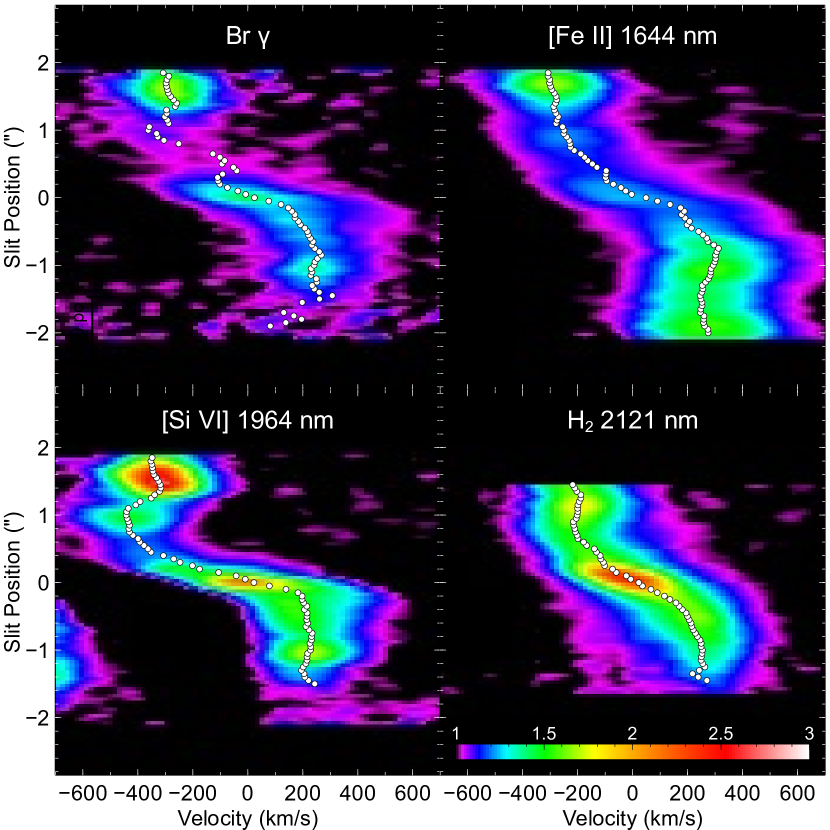
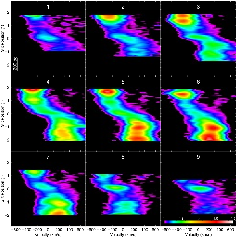
Figure 22: PV diagrams for Br $\gamma$, [Fe II], [Si VI] and H₂, as described in the text. The slit position values are negative in the SE/S direction to positive in the NW/N position. The flux maps have different intensity for contrast enhancement. The LOS velocity derived from the velmap procedure is overlaid as white points. The Br $\gamma$ diagram shows significant discontinuities in the negative velocity outflow vs. the other species; this is also noted for the [O III] emission, as may be due to turbulent entrainment or flickering AGN activity

Figure 23: Off-nucleus PV diagrams for [Fe II] through the outflow. The plots are numbered corresponding to the slits in Fig. 23. The flux maps all have the same intensity scale (color-bar in panel 9).

Figure 24: Off-nucleus PV diagrams for Br $\gamma$ through the cones. The plots are numbered corresponding to the slits in Fig. 23. The flux maps all have the same intensity scale (color-bar in panel 9). There are significant discontinuities, especially in the negative velocity flows; the main ‘hot-spot’ is the impact location on the star-forming ring.

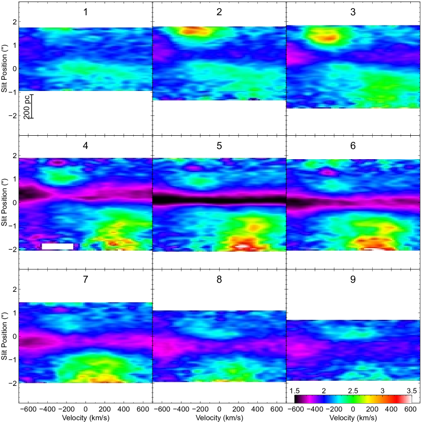
Figure 25: Flux ratio [Fe II]/Br $\gamma$ PV diagrams. The flux ratios all have the same range, given by the color-bar in panel 9. Higher values are where [Fe II] flux is relatively higher than Br $\gamma$; this shows the reduced importance close to the nucleus and increased ratio further along the cones.

4 Discussion

4.1 The Super-massive Black Hole

The black hole mass can be derived using various scaling relationships from observed galaxy parameters. The best-known, and most well-established, uses the stellar velocity dispersion (the $M-\sigma$ relationship). Graham & Scott (2013) gives several scaling values, depending on the galaxy morphology. As it is not clear the exact morphology of the complicated nuclear structure, we will use the regression values for all galaxies in the data set, (with the dispersion $\sigma$ measured in km s^-1):

$$\log(M_{BH})=(8.15\pm 0.05)\\ +(6.07\pm 0.31)~{}\log\left(\dfrac{\sigma}{200}\right)\pm 0.41$$ (2)

We obtained the stellar dispersion for a central 1″ aperture using several method, and compared them with literature values; these are given in Table 2. As can be seen from Fig. 1, the exact choice of aperture can also affect the measured dispersion.

Lin et al. (2018), using the same SINFONI data set, derived the central stellar velocity dispersion of $164\pm 4$ km s^-1 from the CO band-heads. Our solution used the NIFS Gemini spectral library of near-infrared late-type stellar templates (Version 2) (Winge et al., 2009), which has 20 stars observed at 2.13Å, re-binned to 1Å. We used the penalized pixel-fitting (pPXF) method of Cappellari & Emsellem (2004); we found the dispersion to be the same as the Lin et al. (2018) result, within errors.

We also derived the dispersion using the Ca II triplet templates from the Miles SSP models, using the Padova isochrones and the Kroupa Universal initial mass function, for a range of metallicities; this is a suite of 350 template spectra. The pPXF method was again employed. As well, we compared this with the velmap derived dispersion on the Ca II 8544.4Å absorption line.

Table 2: Stellar dispersion derived by different methods.

Spectral line	Source	Method	$\sigma$	$\Delta\sigma$
Ca II triplet	This work	T	156	21
CO band-heads	This work	T	154	26
Ca II 8544.4 Å	This work	V	179	10
Si I 1588.8 nm	This work	V	221	29
CO band-heads	Lin et al. (2018)	T	164	4
Stellar kinematics	Wagner & Appenzeller (1988)	X	210	15
Stellar kinematics	McElroy (1995)	X	209	…
Method (Col. 3): T - template fitting using pPXF - see text for description of template sets.
V - simple Gaussian fit using the velmap procedure from QFitsView.
X - cross-correlation technique of Tonry & Davis (1979).
Dispersion values for this work measured in 1″ radius aperture.

Fitting a single absorption line possibly overestimates the dispersion; the dispersion derived from the cross-correlation technique might also have aperture effects, especially considering the large velocity gradients over the central region. We will use the average of the three pPXF template fitting methods, which gives $158\pm 34$ km s^-1. For comparison, we will also use the value for the Ca II single-line fit.

The exact choice of regression parameters used in the $M-\sigma$ relationship for different galaxy morphologies, is of minor importance, as the errors in the dispersion measurement are dominant in the final calculation of the SMBH mass.

The K-band bulge luminosity relationship ($M-L_{K_{s},sph}$) is of the form:

$$log(M_{BH})=(9.05\pm 0.12)\\ +(-0.44\pm 0.08)~{}\log\left(M+25\right)\pm 0.44$$ (3)

using the parameters from Graham & Scott (2013). The $M-L_{K_{s},sph}$ value was derived from the 2MASS $K_{S}$ image by fitting a 2D Gaussian to the central bulge and measuring the flux in counts, then converting to an absolute magnitude using the photometric zero-point and the distance modulus.

The Sérsic index ($n$) is fitted to the light profile, and has the scaling relationship (Savorgnan et al., 2013):

$$\log(M_{BH})=(8.37\pm 0.3)\\ +(2.23\pm 1.5)~{}\log\left(\dfrac{n}{3}\right)\pm 0.27$$ (4)

The index was fitted to the K continuum flux radial profile from the SINFONI data cube (see Fig. 26). The radial profile shows signs of a turn-over in the inner few pixels, indicative of a ‘core-Sérsic’ profile (see Graham & Scott, 2013; Savorgnan et al., 2013); the Sérsic index fit excludes the inner two points; these points are also below the spatial resolution. We also compared this with the core-Sérsic fit for the 2MASS $K_{S}$ image.

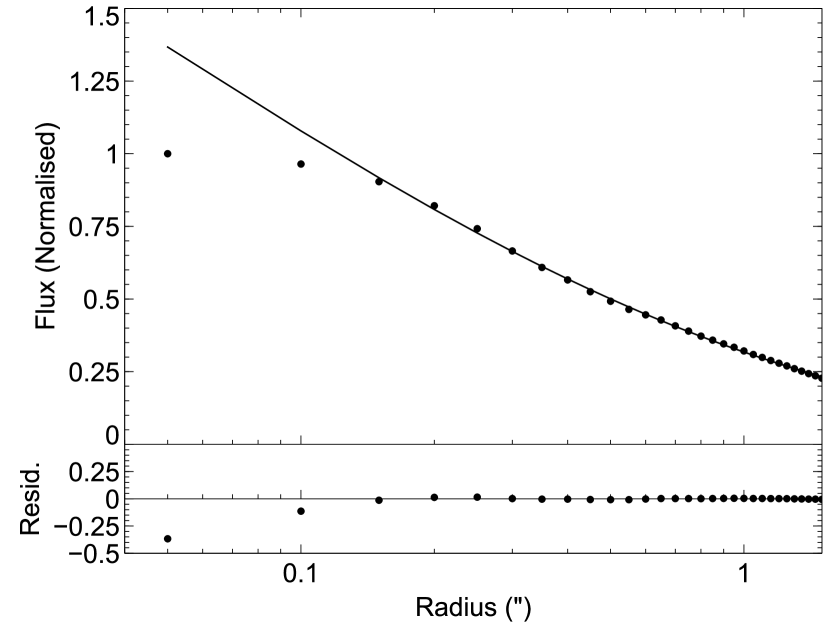
Figure 26: Top panel : radial profile data (points) with the Sérsic fit (index = 3.54). Bottom panel : residual (fit–data). Radius in logarithmic scale, flux is normalized. This implies a SMBH mass of $\sim 3.4\times 10^{8}~{}\rm M_{\odot}$.

The spiral arm pitch angle is related to the SMBH mass in the form (Davis et al., 2017):

$$\log(M_{BH})=(7.01\pm 0.07)\\ -(0.171\pm 0.017)~{}[|\phi|-15\arcdeg]\pm 0.30$$ (5)

where $\phi$ is the spiral pitch angle in degrees. The spiral arm pitch angle was measured from the faint arms that come from the end of the bar, not the ‘Outer Ring’ structure. I thank Dr. Benjamin Davis for providing the data, using the software SPIRALITY (Shields et al., 2015a, b), SpArcFiRe (Davis & Hayes, 2014) and 2DFFT (Davis et al., 2012). The de-projected galaxy image, with the fitted logarithmic spiral arcs, is shown in Fig. 27; the de-projection angle is 43°.

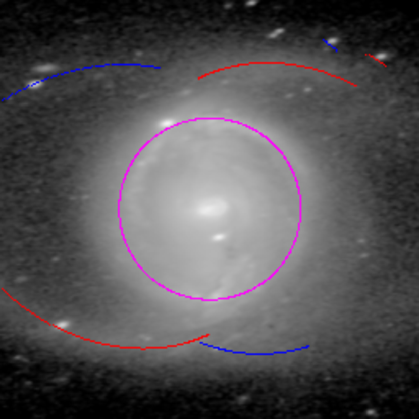
Figure 27: NGC 5728 de-projected image, showing the fitted logarithmic spiral arcs (red and blue) and the ‘Outer Ring’ (magenta circle); the pitch angle relationship gives a SMBH mass of $\sim 3.4\times 10^{8}~{}\rm M_{\odot}$

Table 3 gives the black hole mass measurements determined by the four different methods. The values show a scatter of about 1 dex. The $M-L_{K_{s},sph}$ value has uncertainties due to obscuration and a lack of a well-defined ‘classical’ bulge and the presence of a nuclear bar; obscuration may also affect the derived Sérsic index. We will use the value derived by the template fitting, $\rm M_{\bullet}~{}=~{}3.4(+13.6,-2.7)\times 10^{7}~{}\rm M_{\odot}$. The mass derived from the 2MASS $K_{S}$ image Sérsic index is compatible with this value.

Table 3: SMBH Mass derived from scaling relationships.

Method	Value	log(M∙)	$\rm M_{\bullet}(\times 10^{8}~{}\rm M_{\odot})$
$M-\sigma$	$158\pm 24$ km s-1	$7.53\pm 0.70$	$0.34(+1.36,-0.27)$
$M-\sigma$	$179\pm 10$ km s-1	$7.86\pm 0.43$	$0.72(+1.26,-0.46)$
$M-L_{K_{s},sph}$	$-23.25\pm 0.01$ Mag	$8.13\pm 0.49$	$1.36(+4.2,-0.45)$
$M-n$	3.54	$8.53\pm 0.42$	$3.39(+8.87,-1.3)$
$M-n$	1.56	$7.74\pm 0.59$	$0.55(+2.1,-0.14)$
$M-\phi$	$7.0\pm 0.3\arcdeg$	$8.37\pm 0.37$	$2.34(+3.15,-1.34)$

The ‘sphere of influence’ of a SMBH (i.e. the volume of space over which the gravity of the SMBH dominates those of the stars) is given by the formula:

$$R_{I} =\dfrac{G\textrm{M${}_{\bullet}$}}{\sigma^{2}}$$ (6)

$$R_{I}(pc) =4.305\times 10^{5}~{}\dfrac{\textrm{M${}_{\bullet}$~{}[10${}^{8}$~{}M${}_{\odot}$]}}{\sigma^{2}~{}\textrm{[km~{}s${}^{-1}$]}}$$ (7)

The bolometric luminosity derived from the X-ray flux (Winter et al., 2012), the Eddington luminosity (i.e. the maximum luminosity possible from a SMBH of a given mass), plus the Eddington ratio and the accretion rate, are given by:

$$\log(L_{Bol}) =1.12~{}\log(L_{X}~{}[14-195~{}\rm{keV}])-4.23$$ (8)

$$L_{Edd} =1.3\times 10^{38}~{}\textrm{M${}_{\bullet}$/M${}_{\odot}$}~{}\rm{erg~{}s^{-1}}$$ (9)

$$R_{Edd} =L_{Bol}/L_{Edd}$$ (10)

$$\dot{M}_{acc} =\dfrac{L_{Bol}}{c^{2}\eta}$$ (11)

$$=1.84\times 10^{-46}~{}L_{Bol}~{}[\rm{erg~{}s^{-1}}]$$ (12)

where $L_{X}$ is the X-ray luminosity, $L_{Bol}$ is the bolometric luminosity, M_∙ is the BH mass and $\dot{M}_{acc}$ is the accretion rate. The rate is given in M_⊙ yr^-1 using the constant in Equation 12 and a standard efficiency rate $\eta=0.1$.

Using the 14–195 keV X-ray luminosity from Davies et al. (2015) and SMBH mass calculated above, this gives:

$$L_{X}(14-195) =1.62\times 10^{42}~{}\textrm{erg s${}^{-1}$}$$

$$L_{Bol} =1.46\times 10^{44}~{}\textrm{erg s${}^{-1}$}$$

$$L_{Edd} =4.42~{}(+17.7,-3.04)\times 10^{45}~{}\textrm{erg s${}^{-1}$}$$

$$R_{Edd} =3.3~{}(+7.3,-2.6)\times 10^{-2}$$

$$\dot{M}_{acc} =2.7~{}\times 10^{-2}~{}\textrm{M${}_{\odot}$~{}yr${}^{-1}$}$$

$$R_{I} =5.9~{}\textrm{pc}$$

Eddington ratios have a large range; the trend, as outlined by Ho (2008), is for higher luminosity AGNs to have higher ratios. Ricci et al. (2014), in their discussion of emission line properties in 10 early-type galactic nuclei, noted that $R_{Edd}<10^{-3}$ for all the galaxies that had AGN; however this sample were all LINERs. Storchi-Bergmann et al. (2010) found the ratio for NGC 4151 was 0.012 and Fischer et al. (2015) found 0.12 for Mrk 509 (both Seyfert 1.5); these have a higher bolometric luminosities than NGC 5728. Vasudevan et al. (2010) gives an Eddington ratio for NGC 5728 of 0.028, the same as the value found here. Their range of values of the ratio for the complete sample of 63 Swift/BAT X-ray AGNs are $6\times 10^{-3}\leq R_{Edd}\leq 7.3\times 10^{-2}$. Ho (2008) gives a median $R_{Edd}$ for LLAGN of $1.1\times 10^{-3}$ for Seyfert 1-type galaxies, and $5.9\times 10^{-6}$ for Seyfert 2s; the bolometric luminosity for this galaxy ($1.46\times 10^{44}$ erg s^-1) places it rather above the range for LLAGN.

In summary, NGC 5728 has a moderate-luminosity Seyfert 2 AGN, with Eddington ratio and accretion rate within the range of values found in the literature, powered by SMBH of $3.4\times 10^{7}~{}\rm M_{\odot}$.

4.2 Outflow Modeling and Kinematics

Are the kinematics seen in the ionization cones dominated by outflows or rotations? Following Müller-Sánchez et al. (2011), the main arguments for outflows are:

• The velocity gradients across the field are too high to be explained by a physically reasonable gravitational potential. The velocity field shows a ${\Delta}V~{}\simeq~{}700$ km s^-1 over $\sim$200 pc, which implies an enclosed mass of $\sim 2.2~{}\times~{}10^{9}~{}\rm M_{\odot}$ (see e.g. Das et al., 2007, modelling NGC 1068)

• The NLR and stellar velocity fields are aligned for rotations - this is not the case with this object.

• The approaching (brighter) radio jet is aligned with blue-shifts, as shown by the channel maps presented above.

• Müller-Sánchez et al. (2011) found an anti-correlation between the outflow opening angles and maximum velocities in their fits of 6 (out of 7) Seyfert galaxies, i.e. the narrower the opening angle, the faster the velocities. The values derived in this work are consistent with their data (see below).

• As shown in section 4.2.2, the bicone does not intersect the plane of the inner nuclear ring but does intersect the plane of the main disk. At $>$ 200 pc from the AGN, the [O III] velocity map from the MUSE data shows a re-orientation, taking on the velocity field of the main disk plane, as seen in the stellar Ca II velocity map (Fig. 2). In other words, there are two velocity fields; an outflow close to the AGN and a rotation further out.

• The velocity profile shows signatures of radial acceleration, followed by deceleration. The gas velocity does not asymptotically tend to zero (as would be expected for rotation), but shows ‘coasting’, i.e. reasonably constant velocity of $\pm 100$ km s^-1 after $\sim 300$ pc; this is consistent with the modeling of NGC 1068 and NGC 4151 (Crenshaw & Kraemer, 2000; Crenshaw & al., 2000), as well as Müller-Sánchez et al. (2011) (NGC 1068, NGC 3783, and NGC 7469).

4.2.1 Velocity Models

There are various physical models of the gas kinematics in outflows from AGN. Crenshaw & Kraemer (2000) modeled the outflow NGC 1068 as a hollow bicone, with emitting material evacuated along the axis - the cone walls were clearly visible in the STIS G430L spectrum as a bifurcation. A similar model was applied to NGC 4151 (Das et al., 2005). Bae & Woo (2016) extended this to generalized bicone models, simulating emitted line profiles. They found that velocity dispersion increases as the intrinsic velocity or the bicone inclination increases, while apparent velocity (i.e., velocity shifts with respect to systemic velocity) increases as the amount of dust extinction increases, since dust obscuration makes a stronger asymmetric velocity distribution along the LOS.

Das et al. (2005) also found that the outflow velocities could be modeled heuristically by a linear or square-root law, i.e. the the velocity increases out from the origin to a turn-over point and then decreases back to systemic, in the form $v=kr$ or $v=k\sqrt{r}$ for the acceleration and $v=v_{max}-k^{\prime}r$ or $v=v_{max}-k^{\prime}\sqrt{r}$ for the deceleration, where $k$ and $k^{\prime}$ are constants, $v_{max}$ is the turn-over velocity and $r$ is the radial distance. In their study of AGN outflow systems, Müller-Sánchez et al. (2011) could model their galaxies with a linear acceleration law (except for Circinus), and 3 of them (NGC 1068, NGC 3783, and NGC 7469) with a linear deceleration law. Liu et al. (2015) modeled IRAS F04250–-5718 and Mrk 509 as filled cones with constant velocity, in which case the maximum velocity dispersion would be expected along the bicone axis.

Fischer et al. (2013) modeled the inclination of 53 Seyfert galaxies from NLR kinematics using a full hollow bicone from [O III] imaging and STIS spectroscopy from HST. NGC 5728 kinematics were classified as ‘Ambiguous’, which means that it has anti-symmetric velocities, but could not classified as having a bicone. They explained this as either the two cones are not identical or that the filling factor is not 1 within the hollow cone and zero outside. The PV diagrams presented above show that the outflowing gas does fill the cones.

Following Das et al. (2005), we fitted the outflow velocity map (derived from the Pa $\beta$ velmap procedure) with all combinations of square root and linear accelerations and decelerations. The Pa $\beta$ map is used instead of Br $\gamma$, as it encompasses a larger area and distance from the AGN, with the Br $\gamma$ map only extending to the turnover distance. The best fit was found with the $\sqrt{r}$ proportionality with a turnover velocity of 290 km s^-1 at a distance of 200 pc from the nucleus. Fig. 28 shows the velocity values and fitted profile. As can be seen, the heuristic functional form is not a good fit around the turnover position; the competing forces on the gas of radiation pressure, magnetic fields, nuclear winds, gravity, ISM friction and gas pressure will produce a more complicated functional form than that given here.

Müller-Sánchez et al. (2011) summarizes the state of knowledge of the dynamical models, noting that while drag forces can produce the required deceleration, the acceleration phase is more difficult to explain, with Everett & Murray (2006) suggesting an accelerated wind close to the AGN (at pc scales) subsequently interacting with and accelerating the ISM over several 100 pc. This is similar to the two-stage outflow model of Hopkins & Elvis (2010).

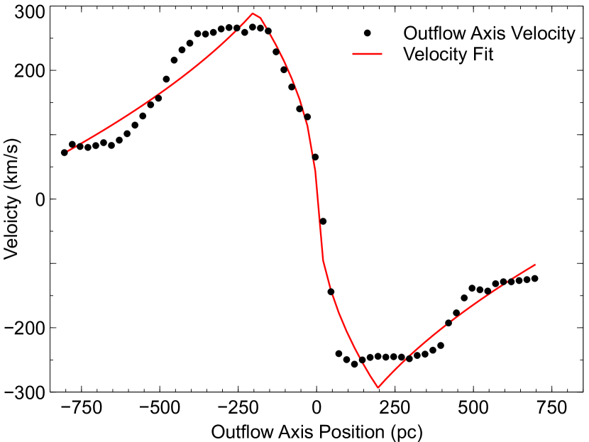
Figure 28: Pa $\beta$ velocity and fitted profile along the outflow axis. The fit is for $\sqrt{r}$ proportionality.

4.2.2 The Bicone Geometry

We further examine the bicone geometry using the channel maps and PV diagrams. The channel map plot for [Fe II] (Fig. 14) shows clear signs of limb-brightening of the outflow (at velocities -337 to +187 km s^-1), which would be expected for a hollow cone model. This is best shown in the velocity range -187 to +37 km s^-1, as the prominent ‘X’-shaped figure with an opening angle of $\sim 70\arcdeg$. The near wall of the approaching cone (-412 to -112 km s^-1) is clearly seen, as is the far wall of the receding cone (+187 to +562 km s^-1). A puzzling aspect in the absence of the far (near) wall in the approaching (receding) cone. It is possible that this has been terminated by the interaction with the plane of the nuclear structure (the inner disk or mini-spiral), and the resulting outflow is a half-cone or fan shape.

By contrast, the Br $\gamma$ channel maps show little sign of the limb brightening, being more like a filled cone; supporting the concept of the [Fe II] jacketing the hydrogen recombination emission. The PV diagrams for Br $\gamma$ (Figs. 23 and 24) also show no or minimal signs of this structure.

If the [Fe II] outflow structure is a hollow bicone, then we should be able to separate the LOS velocities of the front and back walls. Instead of a single Gaussian fit (as from the velmap procedure), the asymmetric line profile of [Fe II] was fitted by a double Gaussian curve, as illustrated for the position 1″ SE of the nucleus (Fig. 30); this shows a double (green dashed line, with blue and red components) vs. a single Gaussian fit (black dashed line). The fits for each pixel along the centerline of the outflow is shown in Fig. 30, top panel, where the black line is the velocity from the velmap procedure, and the blue and red fits are the shorter and longer wavelength of the double Gaussian fits. For the double Gaussian fit, one of the fits always dominates and produces corresponding uncertainties in the other fit, as shown by the error bars. This also corresponds with the low flux of either the far or near wall visibility in the channel maps. The bottom panel of Fig. 30 shows the velmap measured velocity dispersion (i.e. that of the single Gaussian fit), with the uncertainties. Unlike the HST STIS data for NGC 1068 (Crenshaw & Kraemer, 2000), the line profiles do not show bifurcation, just a red or blue skewness.

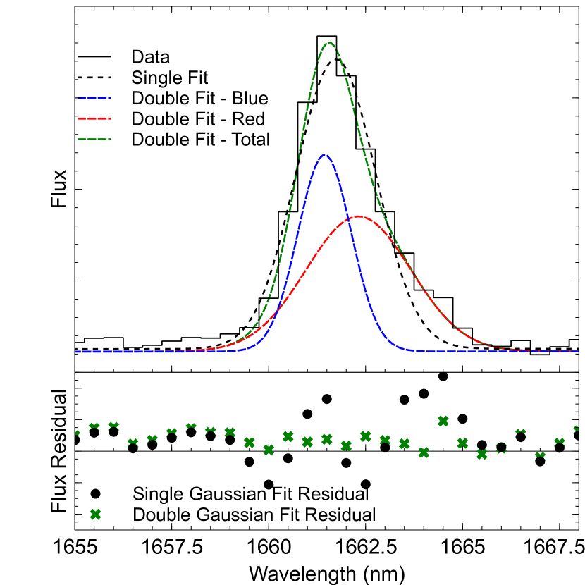
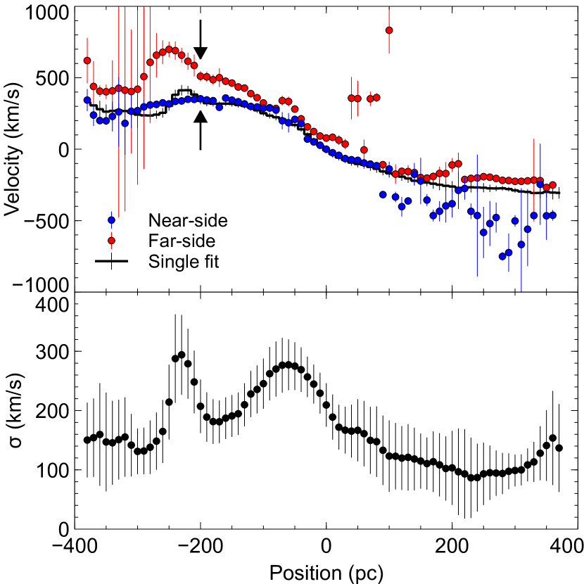
Figure 29: Outflow [Fe II] emission line profiles. Top panel: Single and double Gaussian fit to line profile at position 1″ SE from the nucleus. Bottom panel: Fit residuals from single (black dots) and double (green crosses) Gaussian fits (at the same vertical scale).

Figure 30: [Fe II] kinematics of the front and back wall of hollow bicone outflow. Top panel: Velocities of double Gaussian fit (red and blue points) along the center-line of the outflow, with uncertainties. The black line is the velocity derived from the velmap procedure. The arrows indicate the position for the illustrative double Gaussian fit (Fig. 30). Bottom panel: Velocity dispersion from velmap procedure.

From these velocity measurements, we can derive the outflow bicone parameters of internal opening angle and inclination to the LOS. The outflow is modeled as two cones truncated at the tip, and the sides aligned with the observed limb-brightening; this is shown in Fig. 31 - top left panel, where the colored map is the zero-velocity channel, the thick dashed lines are the sides of the outflow and the thin dotted line is the center-line of the outflow. The blue and red arrows illustrate the approaching and receding cones. The projected opening angle is measured from the zero velocity channel map at $\alpha=71\arcdeg$; this is larger than the value derived for the emission lines by Capetti et al. (1996) (55–65°) but somewhat narrower than the polarized continuum angle (94°); the [Fe II] jacket of the main flow is the source of the higher opening angle.

The cone internal angle, $\beta$, and the inclination, $i$, (where i=0° means that the cone axis is in the plane of the sky and i=90° means that the cone is face-on) can be derived from the following relationships:

$$\tan(90-\beta/2) =\tan(90-\alpha/2)/\cos(i)$$ (13)

$$V =V_{F}/\sin(i-\beta/2)$$ (14)

$$=V_{B}/\sin(i+\beta/2)$$ (15)

where $V_{F}$ and $V_{B}$ are the measured front and back wall LOS velocities and $V$ is the true outflow velocity. The parameters were derived at several points along the outflow center-line, ensuring that the velocity difference $|V_{B}-V_{F}|$ was over 230 km s^-1, where the two Gaussian components were clearly separated. The equations were solved using the ‘GRG Nonlinear’ algorithm, minimizing the difference between the outflow velocity derived from the front and back velocities, with the added check that the derived projected cone opening angle was close to the observed angle.

The results at the several locations along the center-line agree very well, $\beta=50\arcdeg.2\pm 2\arcdeg.2$ and $i=47\arcdeg.6\pm 3\arcdeg.2$. It is noted that this inclination is close to that of the outer disk (48°) as found in Paper I, i.e. the bicone axis is nearly co-planar to the main galactic plane. This is also close to the value for the de-projection angle for the spiral-arm pitch fit (Section 4.1) of 43°. There is no requirement for AGN outflows to align to the galaxy geometry; Nevin et al. (2017), Müller-Sánchez et al. (2011) and Fischer et al. (2013) all find no alignment between outflow and galactic photometric axes.

The biconal interpretation is further supported at the -112 km s^-1 channel map slice, where a cone slice projected at the inclination can be overlaid on the elliptical feature (Fig. 31 - top right panel). In the bottom left panel of Fig. 31, we show a diagram of the bicone seen side-on across the plane of the sky.

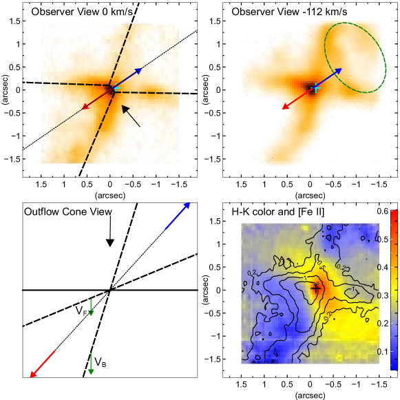
Figure 31: Hollow bicone outflow model. Top left: observer view of outflow boundaries (thick dashed lines) and center-line (thin dotted line), superimposed on the zero velocity channel map. Blue and red arrows indicate approaching and receding outflow velocity directions, the cyan cross indicates the AGN position and the black arrow shows the viewing angle along the plane of the sky for the right panel diagram. Top right: -112 km s^-1 channel map, with overplotted outflow boundary of a cone slice projected to the derived inclination angle of 47°. Bottom left: Side-on (plane of the sky) view of the outflow cones with the lines and blue and red arrows as for the left panel, with the opening angle and inclination as derived. The black arrow is the observer LOS and the green arrows indicate the LOS front and back wall velocities. Bottom right: [Fe II] zero-velocity channel flux (contour) overlaid on the $H-K$ color map. Contour values in 10^-18 erg cm^-2 s^-1, color-bar is $H-K$ values. The association between the dust grain destruction and the [Fe II] emission is shown by the anti-correlation.

Müller-Sánchez et al. (2011) examined the biconal outflows of 7 Seyfert galaxies, and found an anti-correlation between the half-opening angle of the cone and the outflow maximum velocity. The values for NGC 5728 (50° and 260 km s^-1/$\cos{(i)}$ = 380 km s^-1) place it on the trend on the plot (their figure 27) from the objects they measured. They also found an anti-correlation between the H₂ gas mass in the inner 30 pc and the half-opening angle; the H₂ mass for NGC 5728 within that radius is $0.6\times 10^{8}~{}\rm M_{\odot}$, placing it $\sim 0.5$ dex above the trend (their figure 28), but within uncertainties. The correlation between the opening angle and the gas mass (their figure 29) again places NGC 5728 $\sim 0.5$ dex above the trend. They posit that a higher H₂ mass provides increased confinement to the torus, which makes the outflow more highly collimated, which in turn increases the outflow velocity (see also Davies et al., 2006; Hicks et al., 2009; Müller Sánchez et al., 2009).

Fig. 32 shows cartoons of the model using the Shape 3D modeling software (Steffen et al., 2010), using the angular values and sizes derived here and in Paper I. The left panel shows the structures as seen by the observer, the right panel shows the view edge-on to the main galaxy disk. The black disk represents the ‘Main Disk’, with the assumption that the near side is to the NW, the blue (approaching) and red (receding) cones are the outflows and the ‘Inner Disk’ is in green. The left panel shows the galaxy and its structures as seen by the observer, the right panel shows an edge-on view. The model cone length is 1.8 kpc, and the main disk has a 4.8 kpc radius. As can be seen, the bicone, inner disk and main disk axes are not aligned. The outflow axis is almost in the plane of the main disk, with the blue-shifted (approaching) cone just behind the disk from our perspective. This is supported by the dust lanes crossing the outflow on our LOS. The nuclear stellar structure is almost perpendicular to the main disk.

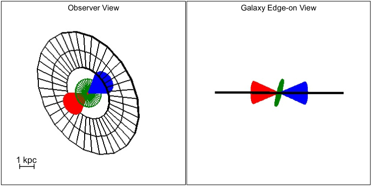
Figure 32: Model cartoon of galactic structure and outflows. Outflows: blue (approaching) and red (receding) cones. Main disk: black. Inner disk: green. Left panel: observer view. Right panel: edge-on to galactic plane view. The skewed morphology for the nuclear stellar structure vs. the main galactic plane is revealed.

It is noted that the condition for visibility of the BLR and thus a Seyfert 1 classification, i.e. $|(i)|+\beta/2>90\arcdeg{}$, is not met, which supports the unified model of AGN, where the nuclear dust structures outside of the BLR collimates the ionizing radiation (see Müller-Sánchez et al., 2011).

As noted in Paper I, the [Fe II] emission is well aligned with the $H-K$ color; this is shown in Fig. 31 - bottom right panel. The edges and other features of the emission flux are anti-correlated with the $H-K$ color (i.e. higher flux as aligned with lower color value). This shows that the dust is being removed at these locations. Alternative mechanisms are mechanical removal through entrainment in the outflows, or the grains being sublimated directly by high-energy photons or sputtered by shocks, releasing the iron to be excited by electron collisions (Mouri et al., 2000). The second process is probably the predominant one, given that the edges delineate the shock boundary of the outflows, as opposed to the lack of correlation between the [Fe II] velocity map and the $H-K$ color map. This is a different mechanism for releasing iron from grains than the standard supernova shock scenario, and is a striking illustration of the process.

4.2.3 Mass Outflow Rate

The maximum outflow velocity observed from Pa $\beta$ of 290 km s^-1 gives a true outflow velocity of $\sim 390$ km s^-1. We derive the mass outflow rate ($\dot{M}_{out}$) using the following procedure. To a first order, the cone can be modeled as a plane, where the LOS velocity and mass surface density represent the integrated chord through the cone. Each spaxel is considered as a cube (0″.05 = 10 pc a side, i.e. 100 pc²/$2\times 10^{-4}$ arcsec²) moving at velocity $V=V_{out}/\sin{(i)}$, where $V_{out}$ is the observed LOS velocity. The mass in the cube is given by Equation 16 (Riffel et al., 2013, 2015)

$$M_{HII}\approx 3\times 10^{17}F_{Br\gamma}D^{2}~{}\rm M_{\odot}$$ (16)

where D is the distance in Mpc and F is the flux of the Br $\gamma$ emission, measured in erg cm^-2 s^-1. This gives the density of hydrogen, which is assumed to be fully ionized in the outflow. (If there is significant mass in the form of neutral and atomic hydrogen in the outflow, this value will be underestimated, as will the corresponding kinetic power. This could be especially true away from the ionizing source, as the gas is coasting.)

Combined with the relationship (accurate to a few percent) of 1 km s^-1 = 1 pc Myr^-1, and the distance of 41.1 Mpc, this gives:

$$\dot{M}_{out}~{}=~{}6.9~{}\times~{}10^{13}~{}V_{out}~{}F_{Br\gamma}~{}\textrm{[M${}_{\odot}$~{}yr${}^{-1}$]}$$ (17)

Fig. 33 shows the map of the outflow rates at each spaxel in the bicone in units of M_⊙ yr^-1. The field has been masked to the cone outline. The total outflow rate over the whole field is 38 M_⊙ yr^-1; the total for just the SE cone is 20 M_⊙ yr^-1, showing that the NW cone is not heavily obscured (i.e. they have similar measured outflow rates). However, the outflow rate distribution in each cone is dissimilar; the SE cone shows that the maximum rate is at $\sim 60$ pc from the AGN, whereas the NW cone has it at the supposed radio jet impact region at $\sim 300$ pc. It is possible that the NW cone has some obscuration from the dust lane and thus has a higher mass outflow rate than that measured.

The ratio of the accretion and outflow rates can also be computed:

$$\dfrac{\dot{M}_{out}}{\dot{M}_{acc}}=38/(2.7\times 10^{-2})=1415$$ (18)

The ratio of the flow rates ($\dot{M}_{out}/\dot{M}_{acc}$) can be compared with the results from Müller-Sánchez et al. (2011), who find a range of $\sim 100-8000$; our value (only exceeded by one of their objects, NGC 2992) supports their conclusion that Seyferts with strong and collimated radio emission are also hosts of powerful outflows of ionized gas. The ratio of outflow energy to bolometric luminosity is also consistent with the Hopkins & Elvis (2010) models.

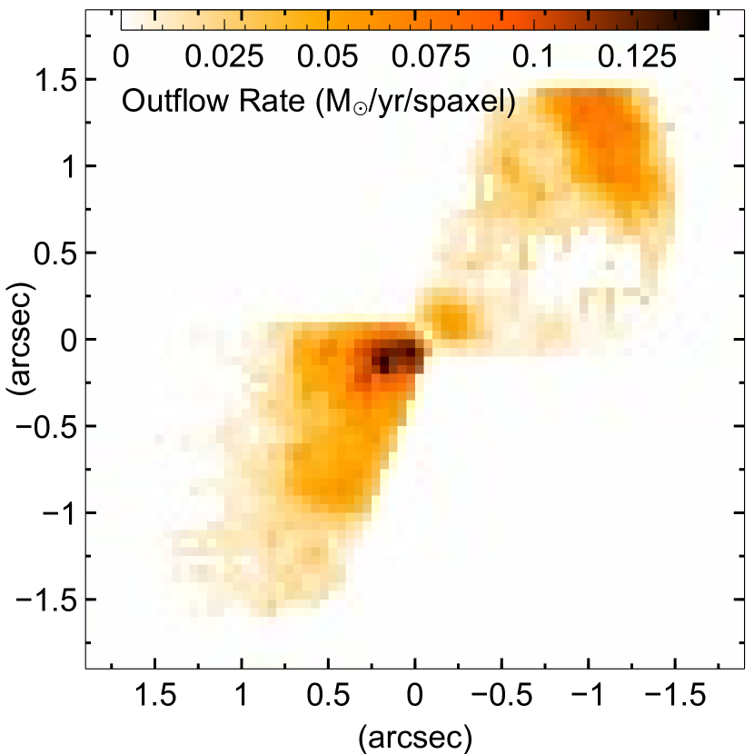
Figure 33: Outflow rate for bicone in M_⊙ yr^-1 spaxel^-1 for hydrogen derived from the Br $\gamma$ flux and velocity fields, showing the SE peak close to the AGN and the NW feature at $\sim 300$ pc where the radio jet impacts the ISM in the SF ring. (One spaxel equals 100 pc², $2.5\times 10^{-4}$ arcsec².)

4.2.4 Outflow Kinetic Power

We compute the kinetic power or luminosity $L_{KE}$ in the outflows (following e.g. Storchi-Bergmann et al., 2010) from Equation 19, which after conversion to cgs units and using Equation 17 becomes Equation 20, where $\dot{M}_{out}$ is in units of M_⊙ yr^-1 and $V_{out}$ and $\sigma$ are in km s^-1. It is assumed that the dispersion measure is due to turbulence; if it is not included the derived power value is reduced by 15%.

$$L_{KE} =\dot{M}_{out}~{}(V^{2}~{}+~{}\sigma^{2})/2$$ (19)

$$=3.15\times 10^{35}~{}\dot{M}_{out}~{}(V_{out}^{2}/\sin^{2}(i)~{}+~{}\sigma^{2})~{}\textrm{erg~{}s${}^{-1}$}$$ (20)

This results in a total kinetic power of $\sim 1.5\times 10^{42}$ erg s^-1, which is $\sim 0.01~{}L_{Bol}$; this is calculated for each pixel’s mass and velocity.

An alternative method of calculating kinetic power is given in Greene et al. (2012) and references therein, where

$$L_{KE}=1.5~{}(\Omega/4\pi)~{}10^{46}~{}R^{2}_{10}~{}v^{3}_{1000}~{}n_{0}~{}\text{erg~{}s${}^{-1}$}\\$$ (22)

where $R_{10}$ (the outflow extent) is in units of 10 kpc, $v_{1000}$ is the expansion velocity in units of 1000 km s^-1, $n_{0}$ is the ISM density in units of cm^-3 and $\Omega/4\pi$ is the covering factor of the outflow in steradians. Taking $R~{}=~{}2$ kpc, $v_{max}~{}=~{}390$km s^-1, the covering factor (for a bicone with opening angle of 50°) = 0.092 and a rough estimate of the ISM density $n_{0}~{}=~{}1$ cm^-3, we derive $L_{KE}=3.2\times 10^{42}$ erg s^-1, very similar to the calculation above. Again, both calculations would underestimate the energetics if there is significant mass loading of neutral and molecular gas.

The gas mass that can be expelled from the galaxy can be estimated, following Storchi-Bergmann et al. (2010). The projected outflow length and average velocity are 2 kpc and 175 km s^-1, respectively, which leads to the AGN active lifetime of at least 10⁷ yr; this means a total kinetic energy of $\sim 5\times 10^{56}$ erg. We use the estimated galaxy mass of $M_{Galaxy}=7.2\times 10^{10}~{}\rm M_{\odot}$ (derived above) and the relationship:

$$M_{Gas}\approx\dfrac{E_{Bind}~{}\times~{}R_{Gas}}{G~{}\times~{}M_{Galaxy}}$$ (23)

where $M_{Gas}$ is the expelled gas mass, $E_{Bind}$ is the total kinetic energy (equated to the binding energy) and $R_{Gas}$ is the observed outflow distance. This equates to $M_{Gas}=1.6\times 10^{8}~{}\rm M_{\odot}$.

This is of the order of the total gas outflow through the bicones over the activity cycle of $\sim 4\times 10^{8}~{}\rm M_{\odot}$, and is also of the order of the estimated mass of molecular gas in the nuclear region ($7\times 10^{8}~{}\rm M_{\odot}$); this indicates that a large proportion of the gas will be blown away by the end of the AGN activity cycle, especially if the AGN lifetime is a few times that given here.

The galaxy mass value given above is likely to be underestimated, since we must include dark matter in the gravitational potential. From Rubin (1980), the rotational velocity is measured at $\sim 175$ km s^-1 at a radius of 11340 pc; given the disk inclination of 60°(a reasonable average of the last two values in Table 3 in Paper I), the circular velocity is $\sim 350$ km s^-1. From simple Keplerian rotation, this gives an enclosed value of $M_{Galaxy}=3.2\times 10^{11}~{}\rm M_{\odot}$, i.e. a ratio of 4.5 over the purely baryonic mass. Substituting this value in Equation 23 gives an expelled gas mass $M_{Gas}=3.6\times 10^{7}~{}\rm M_{\odot}$.

The kinetic-to-bolometric luminosity ratio is larger than values found in Barbosa et al. (2009) for 6 nearby Seyfert galaxies, which were in the range $10^{-5}\leq L_{KE}/L_{Bol}\leq 10^{-4}$; however, it is within the range of the values from Müller-Sánchez et al. (2011), who find $2\times 10^{-4}\leq L_{KE}/L_{Bol}\leq 5\times 10^{-2}$ for 7 Seyfert galaxies with biconal outflows. In general, the former objects did not have collimated outflows and had significantly lower bolometric luminosities ($1\times 10^{42}\leq L_{Bol}\leq 4.6\times 10^{43}$ vs. $5\times 10^{43}\leq L_{Bol}\leq 2.5\times 10^{44}$ erg s^-1). The mass outflow to bolometric luminosity ratio is also compatible with the relationship found by Nevin et al. (2017) from summarized literature values.

The time-scale of the AGN activity implies a causal relationship, i.e. the evacuation of a large proportion of the available gas stops the feeding process and thus the AGN activity ceases. However, we note that the feeding to feedback mass ratios ($\sim 0.1\%$) means that the AGN can be fed equatorially for a period after the polar gas has been expelled.

4.2.5 The Source of The Outflow

Could there be a contribution from nuclear star-formation to the outflow kinematics? Following the arguments from Müller-Sánchez et al. (2011) and Greene et al. (2012) and references therein, we can regard this as unlikely:

• The outflow geometry of starbursts and AGNs is different; star-burst galaxies show hollow truncated cone outflows (see also Durré et al., 2017, for IC 630), whereas this object shows a very small source area.

• The emission-line diagnostics (Paper I), show only AGN excitation at the nucleus (for both optical and infra-red diagnostics), with minimal or no SF mixing.

• Even if all the H II emission was from star formation (which is, of course, inconsistent with the excitation mode deduced from the line ratios), the Br $\gamma$ flux from the central 1″ would imply a SFR = 0.2 M_⊙ yr^-1 (using the flux from Table 5 of Paper I, the distance of 41.1 Mpc and the SFR relationship from Kennicutt et al. (2009) with $T=10^{4}~{}$K and $n_{e}=10^{5}$). Veilleux et al. (2005) gives a relationship between the SFR and the mechanical luminosity of $L_{KE}~{}=~{}7\times 10^{41}~{}(SFR/\text{M${}_{\odot}$~{}yr${}^{-1}$})$ erg s^-1, for solar metallicity and constant mass/energy injection after $\sim 40$ Myr. This gives an energy rate of $1.4\times 10^{41}$ erg s^-1, an order of magnitude below the measured value ($\sim 1.5\times 10^{42}$ erg s^-1).

5 Conclusion

We have examined the nuclear region of NGC 5728 using data at from optical and NIR IFU spectra, revealing a highly complex object showing gas with multiple morphologies and kinematic structures, driven by a powerful AGN. We have presented and analyzed gaseous and stellar kinematics by modeling emission and absorption spectral lines of several species, mapping velocity and dispersion, as well as using PV diagrams and channel maps to resolve kinematic structures.

In summary, the nuclear gas and stellar kinematics present the following features:

• The SMBH mass was determined to be $3.4^{+10.4}_{-2.7}\times 10^{7}$ M_⊙, derived from the $M-\sigma$ relationship. The $M-L_{K_{s},sph}$, $M-n$ and $M-\phi$ relationships produce values up to an order of magnitude higher, but these may have issues related to obscuration and the presence of a nuclear bar.

• The bolometric luminosity of the AGN is $L_{Bol}=1.46\times 10^{44}$ erg s^-1, the Eddington ratio is $E_{Edd}=3.3\times 10^{-2}$ and the mass accretion rate necessary to power the system is $\dot{M}_{acc}=2.7~{}\times 10^{-2}$ M_⊙ yr^-1. The black hole sphere of influence is $\sim 6$ pc.

• The model of an AGN-driven outflow (rather than rotation) is supported by the kinematics, from arguments of radio-jet alignment, non-alignment with the stellar rotation and compatibility of of the velocity and opening angle with other observations of outflows. As the outflow impacts on the main galactic disk far from the AGN, the kinematics show the gas being swept up by the ISM.

• The AGN central engine is obscured behind a broad dust lane; the position was determined by following the trajectory of the brightest pixel across the spectrum, which shows reduced obscuration at longer wavelengths. This deduced location was supported by the position of the base of the outflows as derived from the channel maps.

• The outflow velocity profile was traced using the Pa $\beta$ emission line kinematics, which showed a symmetric bicone pattern, accelerating away from the AGN to a LOS velocity maximum of about -250 km s^-1 at $\sim 220$ pc projected distance to the NW and 270 km s^-1 at $\sim 280$ pc SE of the nucleus, then decelerating to -150/110 km s^-1 at double those distances. The velocity profile was modeled proportionately to the square-root of the distance from the AGN, but this did not fit the turnover well; the multiple competing astrophysical forces (radiation pressure, gravity, winds, gas pressure etc.) will affect the profile.

• The bicone geometry was examined using channel maps; the Br $\gamma$ emission seems to fill the cone, whereas the [Fe II] emission jackets it. Modeling the [Fe II] line profile along the bicone center with a double Gaussian fit, the internal opening angle (50°.2) and the inclination to the LOS (47°.6) were calculated; indicating that the bicone axis is nearly parallel to the plane of the galaxy. This supports the Unified Model of AGN, as these angles preclude seeing the accretion disk, which is obscured by the nuclear-scale dust structures. MUSE data also shows kinematic signatures of impact with the main galactic plane

• There is some evidence that the dust is being removed in the outflows, as seen with the [Fe II] emission being anti-correlated with the H-K color. This could be by entrainment in the outflow or grain sublimation by ionizing radiation or shocks. This is also supported by the reduced extinction observed in the outflows.

• The mass outflow rate through the bicones is estimated at 38 M_⊙ yr^-1; the ratio of outflow rate to the accretion rate required to power the AGN is 1415. The total outflow kinetic power is estimated at $\sim 1.5\times 10^{42}$ erg s^-1, which is 1% of the bolometric luminosity.

• Over the estimated AGN active lifetime of 10⁷ years, the gas mass that can be completely unbound from the galaxies gravity is $1.6\times 10^{8}~{}\rm M_{\odot}$. This is of the order of the total gas outflow through the bicones over the activity cycle ($\sim 4\times 10^{8}~{}\rm M_{\odot}$), and is also of the order of the estimated mass of molecular gas in the nuclear region ($7\times 10^{8}~{}\rm M_{\odot}$). A large proportion of the available gas for star formation can be expelled over the AGN life-cycle.

To understand the complex nature of AGNs, their associated nuclear gas and stars must be studied at the highest resolution possible using multi-messenger observations.

References

- Bae & Woo (2016) Bae, H.-J., & Woo, J.-H. 2016, ApJ, 828, 97
- Barbosa et al. (2009) Barbosa, F. K. B., Storchi-Bergmann, T., Cid Fernandes, R., Winge, C., & Schmitt, H. 2009, MNRAS, 396, 2
- Capetti et al. (1996) Capetti, A., Axon, D. J., Macchetto, F., Sparks, W. B., & Boksenberg, A. 1996, ApJ, 466, 169
- Cappellari & Copin (2003) Cappellari, M., & Copin, Y. 2003, MNRAS, 342, 345
- Cappellari & Emsellem (2004) Cappellari, M., & Emsellem, E. 2004, PASP, 116, 138
- Catinella et al. (2005) Catinella, B., Haynes, M. P., & Giovanelli, R. 2005, AJ, 130, 1037
- Combes & Leon (2002) Combes, F., & Leon, S. 2002, in SF2A-2002, ed. F. Combes & D. Barret (Paris: EDP-Sciences), 1–2
- Crenshaw & al. (2000) Crenshaw, D. M., & al., E. 2000, AJ, 2, 1731
- Crenshaw & Kraemer (2000) Crenshaw, D. M., & Kraemer, S. B. 2000, ApJ, 532, L101
- Das et al. (2007) Das, V., Crenshaw, D. M., & Kraemer, S. B. 2007, ApJ, 656, 699
- Das et al. (2005) Das, V., Crenshaw, D. M., Hutchings, J. B., et al. 2005, AJ, 130, 945
- Davies et al. (2006) Davies, R. I., Thomas, J., Genzel, R., et al. 2006, ApJ, 646, 754
- Davies et al. (2015) Davies, R. I., Burtscher, L., Rosario, D., et al. 2015, ApJ, 806, 127
- Davis et al. (2012) Davis, B. L., Berrier, J. C., Shields, D. W., et al. 2012, ApJSS, 199, 33
- Davis et al. (2017) Davis, B. L., Graham, A. W., & Seigar, M. S. 2017, MNRAS, 471, 2187
- Davis & Hayes (2014) Davis, D. R., & Hayes, W. B. 2014, Am. Astron. Soc., 790, 2
- Diniz et al. (2015) Diniz, M. R., Riffel, R. A., Storchi-Bergmann, T., & Winge, C. 2015, MNRAS, 453, 1727
- Dopita et al. (2015) Dopita, M. A., Shastri, P., Davies, R., et al. 2015, ApJSS, 217, 12
- Durré & Mould (2018) Durré, M., & Mould, J. 2018, ApJ, In press
- Durré et al. (2017) Durré, M., Mould, J., Schartmann, M., Uddin, S. A., & Cotter, G. 2017, ApJ, 838, 102
- Emsellem et al. (2001) Emsellem, E., Greusard, D., Combes, F., et al. 2001, A&A, 368, 52
- Everett & Murray (2006) Everett, J. E., & Murray, N. 2006, ApJ, 656, 13
- Fischer et al. (2013) Fischer, T. C., Crenshaw, D. M., Kraemer, S. B., & Schmitt, H. R. 2013, ApJSS, 209, 1
- Fischer et al. (2015) Fischer, T. C., Crenshaw, D. M., Kraemer, S. B., et al. 2015, ApJ, 799, 234
- Gorkom (1982) Gorkom, J. H. V. 1982, The Messenger, 33, 45
- Graham & Scott (2013) Graham, A. W., & Scott, N. 2013, ApJ, 764, 151
- Greene et al. (2012) Greene, J. E., Zakamska, N. L., & Smith, P. S. 2012, ApJ, 746, 86
- Hicks et al. (2009) Hicks, E. K. S., Davies, R. I., Malkan, M. A., et al. 2009, ApJ, 696, 448
- Ho (2008) Ho, L. C. 2008, ARA&A, 46, 475
- Hopkins & Elvis (2010) Hopkins, P. F., & Elvis, M. 2010, MNRAS, 401, 7
- Kennicutt et al. (2009) Kennicutt, R. C., Hao, C.-N., Calzetti, D., et al. 2009, ApJ, 703, 1672
- Lin et al. (2018) Lin, M.-Y., Davies, R., Hicks, E., et al. 2018, MNRAS, 473, 4582
- Liu et al. (2015) Liu, G., Arav, N., & Rupke, D. S. N. 2015, ApJSS, 221, 9
- McElroy (1995) McElroy, D. B. 1995, ApJSS, 100, 105
- Mediavilla & Arribas (1995) Mediavilla, E., & Arribas, S. 1995, MNRAS, 276, 579
- Mouri et al. (2000) Mouri, H., Kawara, K., & Taniguchi, Y. 2000, ApJ, 528, 186
- Müller Sánchez et al. (2009) Müller Sánchez, F., Davies, R. I., Genzel, R., et al. 2009, ApJ, 691, 749