An Interpretable Generative Model for Handwritten Digit Image Synthesis

Abstract

An interpretable generative model for handwritten digits synthesis is proposed in this work. Modern image generative models, such as Generative Adversarial Networks (GANs) and Variational Autoencoders (VAEs), are trained by backpropagation (BP). The training process is complex and the underlying mechanism is difficult to explain. We propose an interpretable multi-stage PCA method to achieve the same goal and use handwritten digit images synthesis as an illustrative example. First, we derive principal-component-analysis-based (PCA-based) transform kernels at each stage based on the covariance of its inputs. This results in a sequence of transforms that convert input images of correlated pixels to spectral vectors of uncorrelated components. In other words, it is a whitening process. Then, we can synthesize an image based on random vectors and multi-stage transform kernels through a coloring process. The generative model is a feedforward (FF) design since no BP is used in model parameter determination. Its design complexity is significantly lower, and the whole design process is explainable. Finally, we design an FF generative model using the MNIST dataset, compare synthesis results with those obtained by state-of-the-art GAN and VAE methods, and show that the proposed generative model achieves comparable performance.

1 Introduction

Data-driven image synthesis is a popular topic for a variety of vision-based applications nowadays. A great majority of modern image synthesis tasks are accomplished by Generative Adversarial Networks (GANs) and Variational Autoencoders (VAEs). The GAN approach trains two networks at the same time, namely, a generator and a discriminator. They are trained with respect to each other adverserially. The generator takes a random vector as the input and generates an image by adapting network parameters to make synthesized and real ones as close as possible. Their difference is detected by the discriminator. The whole training process is cast as a multi-layer non-convex optimization problem and solved by backpropagation (BP). Although the BP approach provides reasonable results, the whole process is complex and mathematically intractable.

To offer an interpretable image generative model, one idea is to adopt a one-stage whitening and coloring process using the principal component analysis (PCA), which is also known as the Karhunen-Lo$\acute{e}$ve transform (KLT). However, the one-stage transform cannot generate images of high resolution. To overcome this difficulty, we derive a multi-stage PCA by cascading multiple transform stages. It relates input images of correlated pixels to output spectral vectors of uncorrelated components through a multi-stage whitening process. To accomplish the synthesis task, we conduct multi-stage transforms in the reversed order that corresponds to a multi-stage coloring process. The resulting generative model is called a feedforward one since there is no backpropagation used in model parameters determination. The complexity of the feedforward model is low and the whole design process is explainable.

The rest of the paper is organized as follows. Related previous work is reviewed in Sec. 2. One-stage and multi-stage generative models are presented in Secs. 3 and 4, respectively. Experimental results are shown in Sec. 5. Some discussion is made in Sec. 6. Finally, concluding remarks are given in Sec. 7.

2 Review of related work

Generative models are an important topic in computer vision and machine learning. Among many state-of-the-art generative models for image synthesis [1, 2, 3], there are two main stochastic models. They are VAEs and GANs. The VAE [4, 5, 6, 7] is a probablistic graphical model that optimizes the variational lower bound on data likelihood. The GAN system [8] consists of a generator and a discriminator. The generator is optimized to fool the discriminator, and the discriminator is optimized to distinguish real and fake images. There are several GAN variants to improve stability and efficiency [9, 10, 11, 12, 13, 14, 15]. Examples include WGAN, informative GAN, etc. Takuhiro et al. [16] proposed a decision tree controller GAN, which can learn hierarchically interpretable representations without relying on detailed supervision. Huang et al. [17] proposed an introspective variational autoencoder (IntroVAE) model to synthesize high-resolution photographic images. It can conduct self-evaluation of generated images for quality improvement accordingly.

Research on interpretable generative methods for image synthesis is much less. One idea is to examine hierarchical representations for image synthesis. Examples include: [18, 19, 20, 21]. Another idea is to adopt a recursive structure [22, 23, 24, 25, 26]. Recently, Kuo et al. [27, 28, 29, 30] studied interpretable convolutional neural networks (CNNs), and proposed an image synthesis solution based on the Saak transform in [29]. They successfully reconstructed images using Saak coefficients. Here, we conduct image synthesis from random vectors rather than image reconstruction, and present a multi-stage PCA-based generative model for high resolution image synthesis.

3 Generative Model with One-Stage PCA

The block-diagram of a generative model using the one-stage PCA is shown in Fig. 1. It contains a forward transform and an inverse transform. They correspond to the whitening and the color processes, respectively. The training data are used to determine the transform kernels and the distribution of transformed coefficients. Then, the two pieces of information are used for automatic image synthesis.

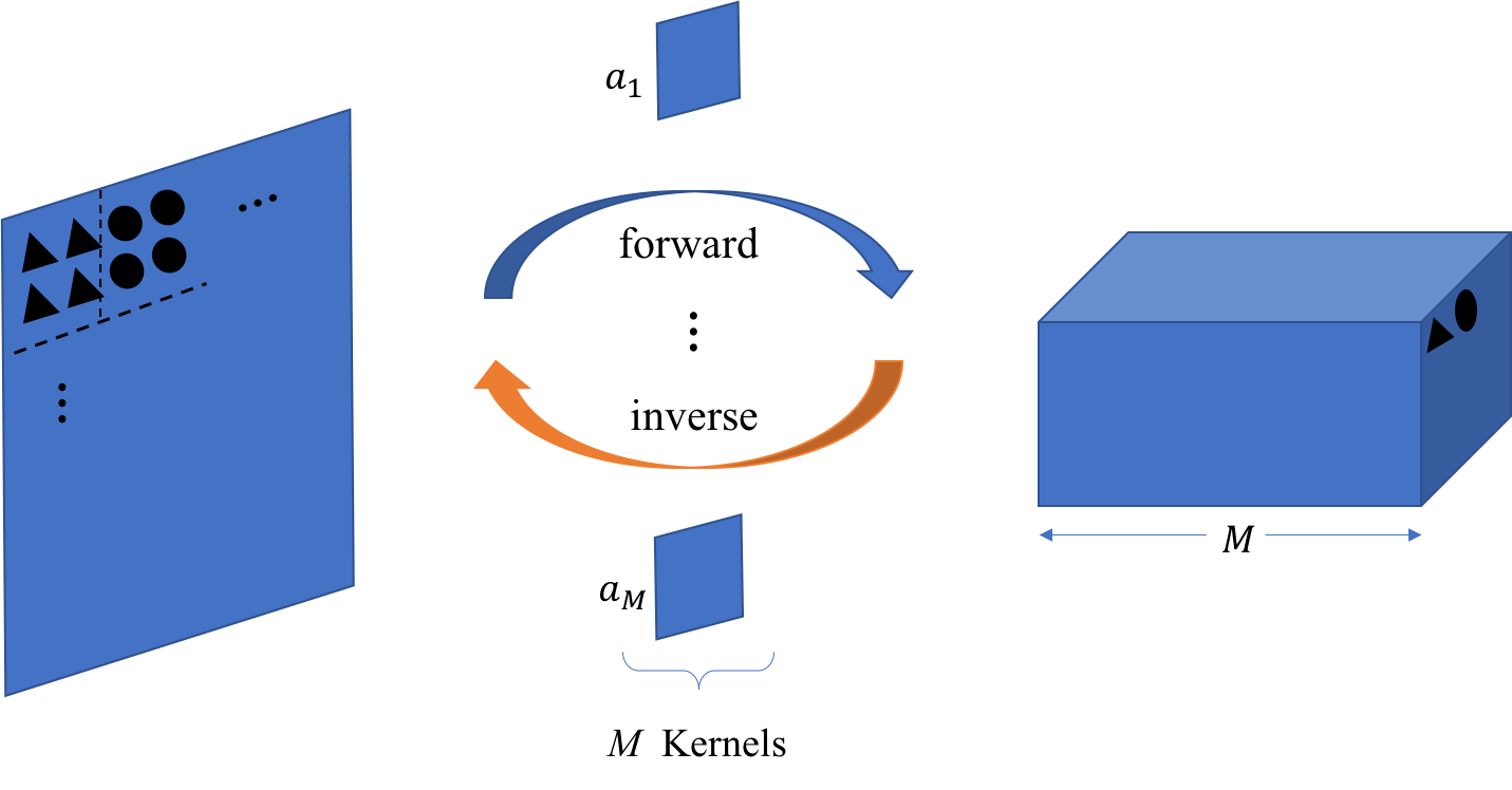
Figure 1: 3D representation of single stage PCA transform. Blue flow represents forward transform, orange flow represents inverse transform.

The forward PCA transform consists of the following two steps.

1. Compute transform kernels from input vectors.
   By following [30], we decompose input vectors into DC (direct current) and AC (alternating current) two components. The correlation matrix for AC input vectors is denoted by ${\bf R}\in R^{N\times N}$. It has rank $N-1$. That is, its first $N-1$ eigenvalues are positive and the last one is zero. The eigenvectors corresponding to positive eigenvalues form an orthonormal basis of the AC subspace. Also, we store eigenvectors in a descent order of its corresponding eigenvalues. We select the first $M$ (with $M\leq N$) eigenvectors, of which its corresponding eigenvalues takes the most energy of the input vector space. The first $M$ basis functions, denoted by ${\bf a}_{1},{\bf a}_{2},\cdots,{\bf a}_{M}$ and called transform kernels, provide the optimal subspace approximation $R^{M}$ to $R^{N}$.

2. Project AC input ${\bf f}$ to kernels ${\bf a}_{1},{\bf a}_{2},\cdots,{\bf a}_{M}$.
   We have projection coefficients shaped in a 3D cuboid, as shown in Fig. 1. The projection coefficients are defined by

   $$p_{i}={\bf a}_{i}^{T}{\bf f},\quad k=1,\cdots,M,$$ (1)

   where ${\bf a}_{i}$, ${\bf f}$ and $M$ denote the $i$th transform kernel, the AC input vector and the number of kernels, respectively.

The inverse PCA transform aims to reconstruct the AC input, ${\bf f}\in R^{N}$, as closely as possible. We use the best linear subspace approximation to reconstruct the input vector using transform kernels ${\bf b}_{i}$, $i=1,\cdots,M$, and projection coefficient vector ${\bf q}=(q_{1},\cdots,q_{M})$. That is, we have

$$\tilde{\bf f}=\sum_{i=1}^{M}q_{i}{\bf b}_{i}.$$ (2)

The inverse PCA transform is a mapping from projection vector ${\bf q}$ to an approximation $\tilde{\bf f}\in R^{M}$ of ${\bf f}\in R^{N}$.

It is worthwhile to highlight two points. First, image synthesis is different from image reconstruction. Image reconstruction attempts to relate one input image with its transformed coefficients. Image synthesis intends to relate one class of images with their transform coefficients. Thus, we should study the distribution of projection coefficient vector ${\bf p}$. It is well known that the PCA transform is a whitening process so that elements of ${\bf p}$ are uncorrelated. Thus, each element can be treated independently. Second, the single-stage PCA cannot generate high quality images of high resolution since many PCA components contain high frequency components only. To address this problem, we proposed to cascade multiple PCA transforms to provide a multi-stage generative model.

4 Generative Model with Multi-Stage PCA

In this section, we propose a generative model based on multi-stage PCA transforms. The block-diagram of the proposed multi-stage generative model is shown in Fig. 2. Since the difference between the original digit images of size $32\times 32$ and the interpolated digit image from size $16\times 16$ to $32\times 32$ is very small, we do an average pooling to reduce all images to size $16\times 16$ as a pre-processing step to save computational complexity. Note that this pre-processing step can be removed to allow a more general processing. We will illustrate this point for more complicated images such as facial images as future extension.

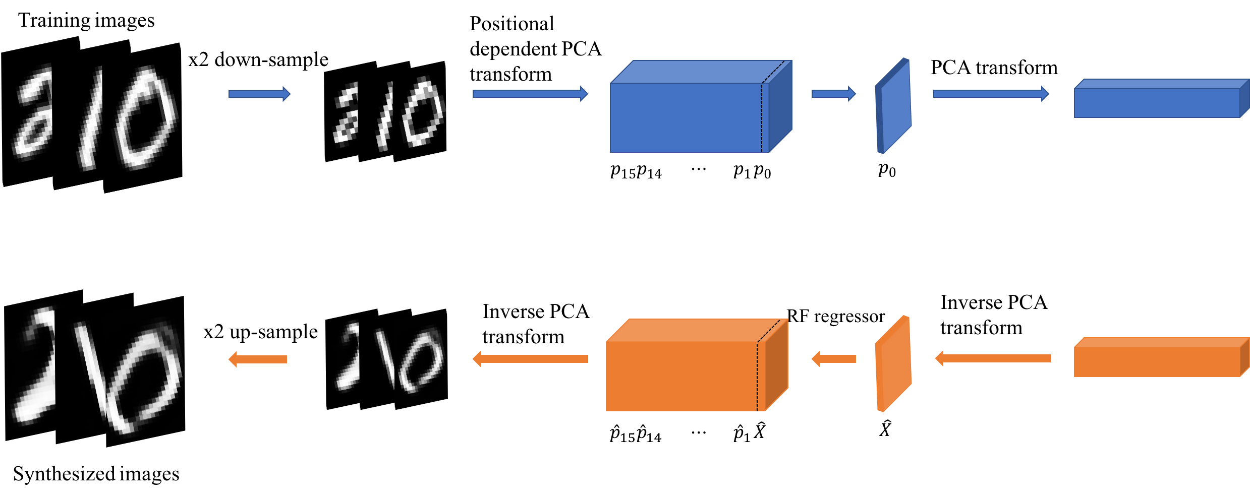
Figure 2: Illustration of the proposed multi-stage generative model for handwritten digits with the MNIST dataset as the training samples, where blue arrows represent the training workflow and orange arrows represent the synthesis workflow.

4.1 Multi-Stage Generative Model

Our proposed system is a two-stage generative model that consists of two single-stage PCA transforms, where the spatial resolution at each stage is $4\times 4$. The model parameters are determined in a FF one-pass manner as follows.

• Stage 1:
  Conduct the position-dependent single-stage PCA transform on non-overlapping batches of size $4\times 4$. Each position yields PCA coefficients of size $16\times 1\times 1$, where $16$ is the spectral component and $1\times 1$ is the spatial resolution. In other words, the 3D cuboid output has the spatial dimension of each position and a spectral dimension of 16. Among 16 spectral coefficients $p_{0},p_{1},\cdots,p_{15}$, $p_{0}$ is the DC projection while others are AC projections. We only pass the DC projection to the second stage and use AC projections of training samples to train a random forest regressor. Then, the random forest regressor will be used to predict AC projections in the synthesis process.

• Stage 2:
  Conduct single-stage PCA transform of dimension $K\times 1\times 1$, where $K$ is the spectral dimension and $1\times 1$ is the spatial dimension. Thus, the whole input image is transformed to a spectral vector of dimension $K$.

The synthesis process is formed by the cascade of two inverse transforms. The input vector is a random vector which has the mean and variance information of PCA coefficients of the last stage. It introduces randomness into the synthesis process.

4.2 Outlier Detection

In the synthesis procedure, a random vector is used as the start point. We may see a synthesized vector that lies in the tail region of the Gaussian distribution. They are outliers and will lead to bad generated samples in the end. We use two methods to detect outliers and remove them. One is k-mean clustering combined with the mean squared error. The other is the Z-score method.

• K-mean clustering and MSE.
  We apply K-mean clustering on coefficients of the second stage PCA. Each cluster has its centroid and the mean squared error. The latter indicates the distance between samples and their centroid. We use $C_{i,k}$ to denote the coefficient of the $i^{th}$ input image in the $k^{th}$ cluster. The centroid for cluster $k$ is $C_{k}^{*}$. Then, we have the mean squared error of cluster $k$:

  $$MSE_{k}=\frac{1}{N_{k}}\sum_{C_{i,k}\in cluster\>k}(C_{i,k}-C_{k}^{*})^{2}$$ (3)

  For each generated $\hat{C}$, we check which cluster it belongs to. If the distance between $\hat{C}$ and its centroid $k$ is greater than $MSE_{k}$, we view it as an outlier, vice versa.

• Z score.
  The Z score is often used to measure the number of standard deviations for a data point to be away from its mean. Here, we use it to detect outliers. Since $C_{i}$ lies in a high dimensional space, we obtain mean $\mu$ and standard deviation $\sigma$ of each dimension. We consider $C_{i}$ as an inlier only if all the components of $C_{i}$ lies within $3\sigma$ range of its distribution.

We discard outliers in the image synthesis process.

4.3 AC Prediction

For the model in Fig. 2, the conditional probability of each AC projection given the DC projection, i.e. $P(p_{i}|p_{0})$, is learned in the training procedure. Thus, in the synthesis flow, once we obtain the generated DC projection, $\hat{X}$, it will be used to predict AC projections through the inverse transform at the second stage. The random forest regressor offers a powerful method in predicting AC projections in two aspects. First, given a set of data points, both input $X$ and output ${\bf b}_{1},{\bf b}_{2},\cdots,{\bf b}_{M}$ are high dimensional, the random forest regressor works well for the dataset. Second, it meets our need. Given $\hat{X}$, the random forest regressor can give the corresponding ${\bf b}_{1},{\bf b}_{2},\cdot,{\bf b}_{M}$.

5 Experimental Results

5.1 Number of Principle Components

For input images of size $\sqrt{N}\times\sqrt{N}$, the total number of principle components is $N$. We choose the first $M$ (with $M<N$) eigenvectors of the correlation matrix to provide the optimal linear subspace approximation, $R^{M}$ to the original space, $R^{N}$. One key question is the selection of parameter $M$. Here, we use the first-stage PCA for the MNIST dataset as an example.

We show the semi-log energy plot of principle components of input images in Fig. 3, where the y-axis indicates the ratio of an eigenvalue $e_{i}$ and the sum of all eigenvalues $\sum e_{i}$, $i=1,2,\cdots,N$, and the x-axis is the indices of principal components. As shown in Fig. 3, the whole energy curve can be decomposed into five linear sectors with four turning points as separators. The four turning points are given in Table 1. To derive these turning points automatically, we use the least square regressor to fit leading data points in one sector and choose the point that starts to deviate from a straight line segment as the turning point.

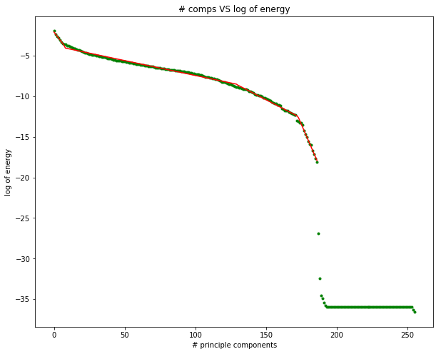
Figure 3: The energy curve as a function of principal component indices for the MNIST dataset.

Table 1: The indices of turning points.

Turning point	1st	2nd	3rd	4th
index	8	120	180	220

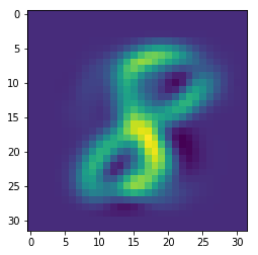
(a) Section 1

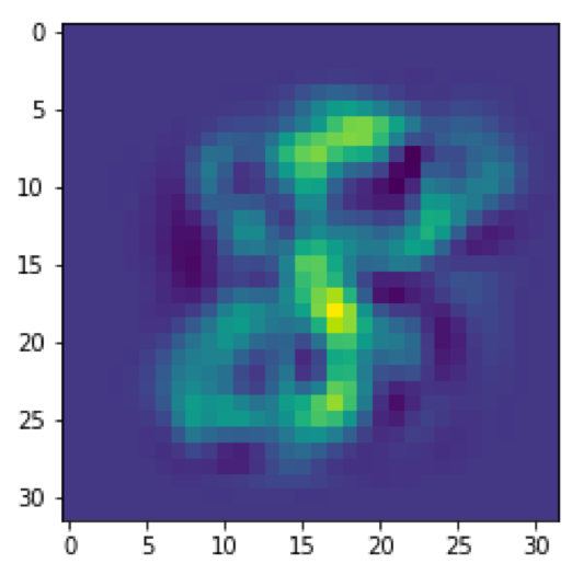
(b) Section 2

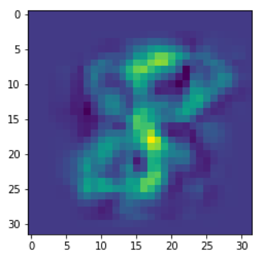
(c) Section 3

Figure 4: Generated images using principle components in different sections.

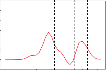
(a) section 1

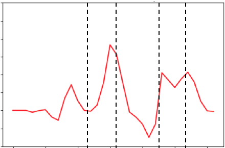
(b) section 2

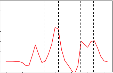
(c) section 3

Figure 5: A horizontal slice of generated image intensity using principle components from different sections, where four dotted lines in each subfigure correspond to the same spatial locations.

In order to understand the role of principal components in each section, we generate images using principal components in each section only and show the result in Fig. 4, where sections 1, 2 and 3 contain principal component indices 1-8, 9-120 and 121-180, respectively. Furthermore, for generated images in Fig. 4, we plot the intensity of a horizontal slice for the corresponding images in Fig. 5, where the horizontal slice is chosen to cross the upper circle of digit 8. We observe a different number of peaks in these three figures. For example, there are only two peaks in Fig. 5(a) representing two peaks in Fig. 4(a). Figs. 5(b) and 5(c) have four peaks, representing four cross points of images in Figs. 4(b) and 4(c), respectively.

Based on the above analysis, we can explain the role of principal components in each section. The first section shapes the main structure of a digit image. The second section enhance the boundary region of the main structure. The third and fourth sections focus on the background, which can be discarded safely. We see that there is a trade-off in the choice of principle components in the second section. If we want to have simpler and clearer stroke images, it is desired to drop components in the second section. However, the variation of generated images will be more limited. It is a trade-off between image quality and image diversity.

5.2 Comparison with GAN and VAE

We validate the proposed image synthesis method using the MNIST handwritten digit dataset. The MNIST dataset is a collection of handwritten digits from 0 to 9. We compare the synthesis results using the proposed method, the VAE and the GAN in Fig. 6. As shown in the figure, we see that our method can generate images that are different from training data with sufficient variations. There is no obvious difference between images synthesized by the three methods. This indicates that our method can perform equally well as the VAE and the GAN but at a lower training cost with a transparent design methodology.

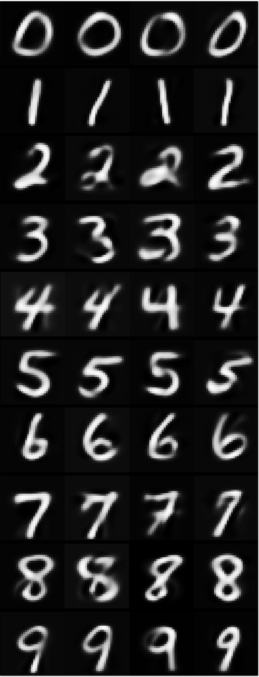
(a) Our method

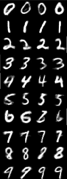
(b) VAE

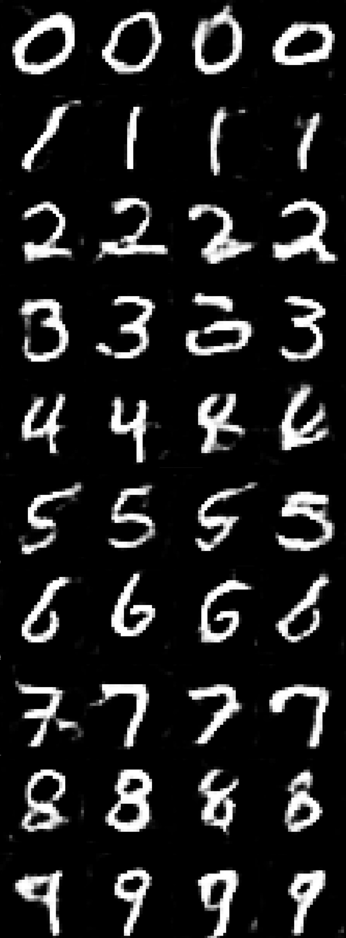
(c) GAN

Figure 6: Comparison of synthesized digits using our method, the VAE and the GAN.

6 Discussion

There are similarities between the proposed generative model and the GAN. First, they both use random vectors for image synthesis. Second, they both use convolutional operations to generate responses and feed them to the next stage. On the other hand, there exist major differences between them as discussed below.

• Theoretical Foundation. It is difficult to explain GAN’s underlying operational mechanism [31, 32]. As compared with the GAN, our proposed method is totally transparent.

• Model Comparison. There are a generator and a discriminator in a GAN. They function as adversaries in the training process. Besides, the BP process is used to determine the model parameters (or filter weights) of both networks. In contrast, our solution does not have the BP dataflow in the training. The training process is FF and one pass.

• Kernel Determination. The filter weights of GANs and VAEs are equivalent to the transformation kernels in our proposed systme. These kernels are determined by the PCA of the corresponding inputs. Our solution is data-centric (rather than system-centric). No optimization framework is used in our solution.

7 Conclusion and Future Work

An interpretable generative model was proposed to synthesize handwritten digits in this work. The multi-stage PCA system was adopted to generate images of high resolution to overcome the drawback of the single-stage PCA system. We discussed how to determine the principle component number in constructing the best linear approximation subspace to the original input space. Also, we presented two methods to detect outliers in the synthesis procedure to improve overall image quality. It was demonstrated by experimental results that our method can offer high quality images that are comparable to those obtained by GAN and VAE at a much lower training complexity since no BP is adopted.

There are several possible directions for further exploration. First, we may design and interpret the VAE based on the proposed framework. The VAE has an encoder and a decoder that have structures similar to ours They correspond the forward transform and the inverse transform respectively. Second, it is inspiring to apply our proposed method to face image synthesis, which is more challenging as compared to handwritten digits. Third, it is worthwhile to study an automatic and effective way to differentiate synthesized and real images. This is critical to image forensic applications.

References

References

- [1] A. Dosovitskiy, J. Tobias Springenberg, T. Brox, Learning to generate chairs with convolutional neural networks, in: Proceedings of the IEEE Conference on Computer Vision and Pattern Recognition, 2015, pp. 1538–1546.
- [2] S. E. Reed, Y. Zhang, Y. Zhang, H. Lee, Deep visual analogy-making, in: Advances in neural information processing systems, 2015, pp. 1252–1260.
- [3] J. Yang, S. E. Reed, M.-H. Yang, H. Lee, Weakly-supervised disentangling with recurrent transformations for 3d view synthesis, in: Advances in Neural Information Processing Systems, 2015, pp. 1099–1107.
- [4] D. P. Kingma, M. Welling, Auto-encoding variational bayes, arXiv preprint arXiv:1312.6114.
- [5] D. J. Rezende, S. Mohamed, D. Wierstra, Stochastic backpropagation and approximate inference in deep generative models, arXiv preprint arXiv:1401.4082.
- [6] A. v. d. Oord, N. Kalchbrenner, K. Kavukcuoglu, Pixel recurrent neural networks, arXiv preprint arXiv:1601.06759.
- [7] S. Zhao, J. Song, S. Ermon, Learning hierarchical features from generative models, arXiv preprint arXiv:1702.08396.
- [8] I. Goodfellow, J. Pouget-Abadie, M. Mirza, B. Xu, D. Warde-Farley, S. Ozair, A. Courville, Y. Bengio, Generative adversarial nets, in: Advances in neural information processing systems, 2014, pp. 2672–2680.
- [9] M. Arjovsky, L. Bottou, Towards principled methods for training generative adversarial networks, arXiv preprint arXiv:1701.04862.
- [10] M. Arjovsky, S. Chintala, L. Bottou, Wasserstein generative adversarial networks, in: International Conference on Machine Learning, 2017, pp. 214–223.
- [11] I. Gulrajani, F. Ahmed, M. Arjovsky, V. Dumoulin, A. C. Courville, Improved training of wasserstein gans, in: Advances in Neural Information Processing Systems, 2017, pp. 5767–5777.
- [12] X. Mao, Q. Li, H. Xie, R. Y. Lau, Z. Wang, S. P. Smolley, Least squares generative adversarial networks, in: Computer Vision (ICCV), 2017 IEEE International Conference on, IEEE, 2017, pp. 2813–2821.
- [13] A. Radford, L. Metz, S. Chintala, Unsupervised representation learning with deep convolutional generative adversarial networks, arXiv preprint arXiv:1511.06434.
- [14] T. Salimans, I. Goodfellow, W. Zaremba, V. Cheung, A. Radford, X. Chen, Improved techniques for training gans, in: Advances in Neural Information Processing Systems, 2016, pp. 2234–2242.
- [15] J. Zhao, M. Mathieu, Y. LeCun, Energy-based generative adversarial network, arXiv preprint arXiv:1609.03126.
- [16] T. Kaneko, K. Hiramatsu, K. Kashino, Generative adversarial image synthesis with decision tree latent controller, in: Proceedings of the IEEE Conference on Computer Vision and Pattern Recognition, 2018, pp. 6606–6615.
- [17] H. Huang, Z. Li, R. He, Z. Sun, T. Tan, Introvae: Introspective variational autoencoders for photographic image synthesis, arXiv preprint arXiv:1807.06358.
- [18] H. Zhang, T. Xu, H. Li, S. Zhang, X. Huang, X. Wang, D. Metaxas, Stackgan: Text to photo-realistic image synthesis with stacked generative adversarial networks, arXiv preprint.
- [19] X. Wang, A. Gupta, Generative image modeling using style and structure adversarial networks, in: European Conference on Computer Vision, Springer, 2016, pp. 318–335.
- [20] C. Vondrick, H. Pirsiavash, A. Torralba, Generating videos with scene dynamics, in: Advances In Neural Information Processing Systems, 2016, pp. 613–621.
- [21] X. Huang, Y. Li, O. Poursaeed, J. E. Hopcroft, S. J. Belongie, Stacked generative adversarial networks., in: CVPR, Vol. 2, 2017, p. 3.
- [22] S. A. Eslami, N. Heess, T. Weber, Y. Tassa, D. Szepesvari, G. E. Hinton, et al., Attend, infer, repeat: Fast scene understanding with generative models, in: Advances in Neural Information Processing Systems, 2016, pp. 3225–3233.
- [23] K. Gregor, I. Danihelka, A. Graves, D. J. Rezende, D. Wierstra, Draw: A recurrent neural network for image generation, arXiv preprint arXiv:1502.04623.
- [24] D. J. Im, C. D. Kim, H. Jiang, R. Memisevic, Generating images with recurrent adversarial networks, arXiv preprint arXiv:1602.05110.
- [25] H. Kwak, B.-T. Zhang, Generating images part by part with composite generative adversarial networks, arXiv preprint arXiv:1607.05387.
- [26] J. Yang, A. Kannan, D. Batra, D. Parikh, Lr-gan: Layered recursive generative adversarial networks for image generation, arXiv preprint arXiv:1703.01560.
- [27] C.-C. J. Kuo, Understanding convolutional neural networks with a mathematical model, Journal of Visual Communication and Image Representation 41 (2016) 406–413.
- [28] C.-C. J. Kuo, The cnn as a guided multilayer recos transform [lecture notes], IEEE Signal Processing Magazine 34 (3) (2017) 81–89.
- [29] C.-C. J. Kuo, Y. Chen, On data-driven saak transform, Journal of Visual Communication and Image Representation 50 (2018) 237–246.
- [30] C.-C. J. Kuo, M. Zhang, S. Li, J. Duan, Y. Chen, Interpretable convolutional neural networks via feedforward design, arXiv preprint arXiv:1810.02786.
- [31] M. Soltanolkotabi, A. Javanmard, J. D. Lee, Theoretical insights into the optimization landscape of over-parameterized shallow neural networks, IEEE Transactions on Information Theory.
- [32] T. Wiatowski, H. Bölcskei, A mathematical theory of deep convolutional neural networks for feature extraction, IEEE Transactions on Information Theory 64 (3) (2018) 1845–1866.