Four-Dimensonal Gauss-Bonnet Gravity Without Gauss-Bonnet Coupling to Matter – Spherically Symmetric Solutions, Domain Walls and Spacetime Singularities

Four-Dimensonal Gauss-Bonnet GravityE. Guendelman, E. Nissimov and S. Pacheva

Eduardo Guendelman1,2,3, Emil Nissimov4, Svetlana Pacheva4

1

2

3

4

We discuss a new extended gravity model in ordinary $D=4$ spacetime dimensions, where an additional term in the action involving Gauss-Bonnet topological density is included without the need to couple it to matter fields unlike the case of ordinary $D=4$ Gauss-Bonnet gravity models. Avoiding the Gauss-Bonnet density becoming a total derivative is achieved by employing the formalism of metric-independent non-Riemannian spacetime volume-forms. The non-Riemannian volume element triggers dynamically the Gauss-Bonnet scalar to become an arbitrary integration constant on-shell. We describe in some detail the class of static spherically symmetric solutions of the above modified $D=4$ Gauss-Bonnet gravity including solutions with deformed (anti)-de Sitter geometries, black holes, domain walls and Kantowski-Sachs-type universes. Some solutions exhibit physical spacetime singular surfaces not hidden behind horizons and bordering whole forbidden regions of space. Singularities can be avoided by pairwise matching of two solutions along appropriate domain walls. For a broad class of solutions the corresponding matter source is shown to be a special form of nonlinear electrodynamics whose Lagrangian $L(F^{2})$ is a non-analytic function of $F^{2}$ (the square of Maxwell tensor $F_{\mu\nu}$), i.e., $L(F^{2})$ is not of Born-Infeld type.

04.50.Kd, 04.70.Bw, 98.80.Cq,

1 Introduction

In the last decade or so a host of problems of primary importance in cosmology (problems of dark energy and dark matter), quantum field theory in curved spacetime (renormalization in higher loops) and string theory (low-energy effective field theories) motivated a very active development of extended gravity theories as alternatives/generalizations of the standard Einstein General Relativity (for detailed accounts, see Refs.[1, 2, 3, 4] and references therein).

One possible approach towards alternative/extended theories to General Relativity is to employ the formalism of non-Riemannian spacetime volume-forms (alternative metric-independent generally covariant volume elements or spacetime integration measure densities) in the pertinent Lagrangian actions, defined in terms of auxiliary antisymmetric tensor gauge fields of maximal rank, instead of the canonical Riemannian volume element given by the square-root of the determinant of the Riemannian metric. The systematic geometrical formulation of the non-Riemannian volume-form approach was given in Refs.[5, 6], which is an extension of the originally proposed method [7, 8].

This formalism is the basis for constructing a series of extended gravity-matter models describing unified dark energy and dark matter scenario [9], quintessential cosmological models with gravity-assisted and inflaton-assisted dynamical generation or suppression of electroweak spontaneous symmetry breaking and charge confinement [10, 11, 12], and a novel mechanism for the supersymmetric Brout-Englert-Higgs effect in supergravity [5].

Let us recall that in standard generally-covariant theories (with actions of the form $S=\int d^{D}\!x\sqrt{-g}{\mathcal{L}}$) the standard Riemannian spacetime volume-form $\omega$ is defined through the “D-bein” (frame-bundle) canonical one-forms $e^{A}=e^{A}_{\mu}dx^{\mu}$ ($A=0,\ldots,D-1$), related to the Riemannian metric ($g_{\mu\nu}=e^{A}_{\mu}e^{B}_{\nu}\eta_{AB}$ , $\eta_{AB}\equiv{\rm diag}(-1,1,\ldots,1)$):

$$\omega=e^{0}\wedge\ldots\wedge e^{D-1}=\det\|e^{A}_{\mu}\|\,dx^{\mu_{1}}\wedge\ldots\wedge dx^{\mu_{D}}\;,$$

so that the Riemannian volume element reads:

$$\Omega\equiv\det\|e^{A}_{\mu}\|\,d^{D}x=\sqrt{-\det\|g_{\mu\nu}\|}\,d^{D}x\;.$$ (1)

Instead of $\sqrt{-g}$ we will employ below a different alternative non-Riemannian volume element given by a non-singular exact $D$-form $\omega=d{\mathcal{C}}$ where:

$${\mathcal{C}}=\frac{1}{(D-1)!}C_{\mu_{1}\ldots\mu_{D-1}}dx^{\mu_{1}}\wedge\ldots\wedge dx^{\mu_{D-1}}\;,$$ (2)

so that the non-Riemannian volume element becomes:

$$\Omega\equiv\Phi(C)d^{D}x=\frac{1}{(D-1)!}\varepsilon^{\mu_{1}\ldots\mu_{D}}\,\partial_{\mu_{1}}C_{\mu_{2}\ldots\mu_{D}}d^{D}x\;.$$ (3)

Here $C_{\mu_{1}\ldots\mu_{D-1}}$ is an auxiliary rank $(D-1)$ antisymmetric tensor gauge field. $\Phi(C)$ is in fact the density of the dual of the rank $D$ field-strength $F_{\mu_{1}\ldots\mu_{D}}=\frac{1}{(D-1)!}\partial_{[\mu_{1}}C_{\mu_{2}\ldots\mu_{D}]}=-\varepsilon_{\mu_{1}\ldots\mu_{D}}\Phi(C)$. Like $\sqrt{-g}$, $\Phi(C)$ similarly transforms as scalar density under general coordinate reparametrizations.

Now, we observe that if we replace the usual Riemannian volume element density $\sqrt{-g}$ with a non-Riemannian one $\Phi(C)$ (3) in the Lagrangian action integral over the 4-dimensional Gauss-Bonnet scalar $\int d^{4}x\,\Phi(C)\,R^{2}_{\rm GB}$ (cf. Eqs.(4)-(5) below), then the latter will cease to be a total derivative in $D=4$. In this way we will avoid the necessity to couple $R^{2}_{\rm GB}$ in $D=4$ directly to matter fields or to use nonlinear functions of $R^{2}_{\rm GB}$ unlike the usual $D=4$ Einstein-Gauss-Bonnet gravity. For reviews of the latter, see Refs.[13, 14]; for recent discussions of Gauss-Bonnet cosmology, see Refs.[15]-[24], and references therein.

Our non-standard $D=4$ Gauss-Bonnet gravity with a Gauss-Bonnet action term $\int d^{4}x\,\Phi(C)R^{2}_{\rm GB}$ has the following principal properties:

• The equation of motion w.r.t. auxiliary tensor gauge field $C_{\mu_{1}\ldots\mu_{D-1}}$ defining $\Phi(C)$ (3) dynamically triggers the Gauss-Bonnet scalar $R^{2}_{\rm GB}$ to be on-shell an arbitrary integration constant (Eq.(15) below).

• Now the composite field $\chi=\frac{\Phi(C)}{\sqrt{-g}}$ appears as an additional physical field degree of freedom related to the geometry of spacetime. Let us note that the latter is in sharp contrast w.r.t. other extended gravity-matter models constructed in terms of (one or several) non-Riemannian volume-forms [5, 6, 9, 10, 11, 12], where we start within the first-order (Palatini) formalism and where composite fields of the type of $\chi$ (ratios of non-Riemannian to Riemannian volume element densities) turn out to be (almost) pure gauge (non-propagating) degrees of freedom, the only remnants being the appearance of some further free integration constants.

The dynamically triggered constancy of $R^{2}_{\rm GB}$ in our modified $D=4$ Gauss-Bonnet gravity has several interesting implications for cosmology [25], in particular, the additional degree of freedom $\chi$ absorbing completely the effect of the matter dynamics within the Friedmann-Lemaitre-Robertson-Walker formalism. The above properties are the most significant differences of the present approach w.r.t. the approach in several recent papers [26, 27, 28], which extensively study static spherically symmetric solutions in gravitational theories in the presence of a constant Gauss-Bonnet scalar. In the latter papers the constancy of the Gauss-Bonnet scalar is imposed as an additional condition on-shell beyond the standard equations of motion resulting from an action principle. Therefore, the full set of equations (equations of motion plus the ad hoc imposed constancy of $R^{2}_{\rm GB}$) in the latter papers is not equivalent to the full set of equations of motion in the present modified $D=4$ Gauss-Bonnet gravity based on the non-Riemannian spacetime volume-form formalism.

The plan of the paper is as follows. After presenting in Section 2 the basics of the non-Riemannian volume-form formulation of modified $D=4$ Gauss-Bonnet gravity, in Section 3 we describe the general properties of the whole class of static spherically symmetric solutions for the various values of the pertinent free integration constants.

In Section 4 we analyze in some detail the domains of definition of the static spherically symmetric metrics and the locations of physical spacetime singularities, domain walls and horizons. The spacetime singularities of the modified $D=4$ Gauss-Bonnet gravity are constant $r=r_{*}$ surfaces bordering whole forbidden space regions of finite or infinitely large extent where the metric becomes complex. Most of these spacetime singularities are not hidden behind horizons. They resemble the so called branch singularities at finite $r$ of static spherically symmetric solutions in higher-dimensional ($D\geq 5$) Einstein-Maxwell-Gauss-Bonnet gravity [29] where the higher-dimensional quadratic curvature invariants exhibit the same singular behaviour near $r_{*}$ as in the present case (cf. Eq.(42) below).

Section 5 contains the graphical representations of the whole class of static spherically symmetric solutions. In Section 6 we briefly illustrate how to avoid spacetime singularities via pairwise matching of two solutions along appropriate domain wall. In the last discussion Section 7 we add some comments and conclusions.

2 Gauss-Bonnet Gravity in $D=4$ With a Non-Riemannian Volume Element

We propose the following self-consistent action of $D=4$ Gauss-Bonnet gravity without the need to couple the Gauss-Bonnet scalar to some matter fields (for simplicity we are using units with the Newton constant $G_{N}=1/16\pi$):

$$S=\int d^{4}x\sqrt{-g}\Bigl{[}R+L_{\rm matter}\Bigr{]}+\int d^{4}x\,\Phi(C)\,R_{\rm GB}^{2}\;.$$ (4)

Here the notations used are as follows:

• $R_{\rm GB}^{2}$ denotes the Gauss-Bonnet scalar:

  $$R_{\rm GB}^{2}\equiv R^{2}-4R_{\mu\nu}R^{\mu\nu}+R_{\mu\nu\kappa\lambda}R^{\mu\nu\kappa\lambda}\;.$$ (5)

• $\Phi(C)$ denotes a non-Riemannian volume element density defined as a scalar density of the dual field-strength of an auxiliary antisymmetric tensor gauge field of maximal rank $C_{\mu\nu\lambda}$:

  $$\Phi(C)=\frac{1}{3!}\varepsilon^{\mu\nu\kappa\lambda}\partial_{\mu}C_{\nu\kappa\lambda}\;.$$ (6)

  Let us particularly stress that, although we stay in $D=4$ spacetime dimensions and although we don’t couple the Gauss-Bonnet scalar (5) to the matter fields, the last term in (4) thanks to the presence of the non-Riemannian volume element (6) is non-trivial (not a total derivative as with the ordinary Riemannian volume element $\sqrt{-g}$)) and yields a non-rivial contribution to the Einstein equations (Eqs.(10) below).

• As we will see in what follows, the specific form of the matter Lagrangian $L_{\rm matter}$ in (4) will depend on the specific class of static spherically symmetric (SSS) solutions we are looking for

      (i) For a broad class of SSS solutions specified below (see Eqs.(36)-(38) below) $L_{\rm matter}$ will be required by consistency of the equations of motion to be a Lagrangian of a nonlinear electrodynamics $L(F^{2})$:

  $$L_{\rm matter}=L(F^{2})\quad,\quad F^{2}\equiv F_{\mu\nu}F_{\kappa\lambda}g^{\mu\kappa}g^{\nu\lambda}\quad,\;\;F_{\mu\nu}=\partial_{\mu}A_{\nu}-\partial_{\nu}A_{\mu}\;.$$ (7)

  An important property of $L(F^{2})$ we prove below is that the latter must be a non-analytic function of $F^{2}$.

      (ii) A special narrow class of SSS solutions (Eq.(29) below) will require “hedgehog” scalar field matter source with a Lagrangian of a $O(3)$ nonlinear sigma-model ($\lambda$ being a Lagrange multiplier) with a “hedgehog” solution [30]:

  $$L_{\rm matter}=-\frac{1}{2}g^{\mu\nu}\partial_{\mu}\vec{\phi}.\partial_{\nu}\vec{\phi}-\lambda\bigl{(}\vec{\phi}.\vec{\phi}-v^{2}\bigr{)}\quad,\quad\vec{\phi}=\pm v\hat{r}\;.$$ (8)

  with $\hat{r}$ – unit radial vector.

      (iii) Another set of SSS solutions require matter sources lacking explicit Lagrangian action formulation, including additional thin-shell (brane) ones describing domain walls (Eqs.(44)-(47) below).

We now have three types of equations of motion resulting from the action (4):

• Einstein equations w.r.t. $g^{\mu\nu}$ where we employ the definition for a composite field:

  $$\chi\equiv\frac{\Phi(C)}{\sqrt{-g}}$$ (9)

  representing the ratio of the non-Riemannian to the standard Riemannian volume element densities:

  $$R_{\mu\nu}-\frac{1}{2}g_{\mu\nu}R=\frac{1}{2}T_{\mu\nu}-\frac{1}{2}g_{\mu\nu}\chi R_{\rm GB}^{2}+2R\nabla_{\mu}\nabla_{\nu}\chi$$

  $$+4\Box\chi\bigl{(}R_{\mu\nu}-\frac{1}{2}g_{\mu\nu}R\bigr{)}-4R_{\mu}^{\rho}\nabla_{\rho}\nabla_{\nu}\chi-4R_{\nu}^{\rho}\nabla_{\rho}\nabla_{\mu}\chi$$

  $$+4g_{\mu\nu}R^{\rho\sigma}\nabla_{\rho}\nabla_{\sigma}\chi-4g^{\kappa\rho}g^{\lambda\sigma}R_{\mu\kappa\nu\lambda}\nabla_{\rho}\nabla_{\sigma}\chi\;,\;\;\;$$ (10)

  where $T_{\mu\nu}=g_{\mu\nu}L_{\rm matter}-2\frac{\partial}{\partial g^{\mu\nu}}L_{\rm matter}$ is the relevant standard matter energy-momentum tensor. In particular, for the nonlinear electrodynamics:

  $$T_{\mu\nu}=g_{\mu\nu}L(F^{2})-4L^{\prime}(F^{2})F_{\mu\kappa}F_{\nu\lambda}g^{\kappa\lambda}\;,$$ (11)

  where $L^{\prime}(F^{2})\equiv\frac{\partial L}{\partial F^{2}}$, and for the scalar “hedgehog” field ${\vec{\phi}}$:

  $$T_{\mu\nu}=\partial_{\mu}\vec{\phi}.\partial_{\nu}\vec{\phi}-\frac{1}{2}g_{\mu\nu}g^{\kappa\lambda}\partial_{\kappa}\vec{\phi}.\partial_{\lambda}\vec{\phi}\;.$$ (12)

• The equations of motion w.r.t. scalar “hedgehog” field ${\vec{\phi}}$ and the nonlinear gauge field have the standard form (they are not affected by the presence of the Gauss-Bonnet term):

  $$\Box{\vec{\phi}}-\lambda{\vec{\phi}}=0\quad,\quad\vec{\phi}.\vec{\phi}-v^{2}=0\;,$$ (13)

  $$\nabla_{\nu}\bigl{(}L^{\prime}(F^{2})F^{\mu\nu}\bigr{)}=0\;.$$ (14)

• The crucial new feature are the equations of motion w.r.t. auxiliary non-Riemannian volume element tensor gauge field $C_{\mu\nu\lambda}$:

  $$\partial_{\mu}R_{\rm GB}^{2}=0\quad\longrightarrow\quad R_{\rm GB}^{2}=24M={\rm const}\;,$$ (15)

  where $M$ is an arbitrary dimensionful integration constant and the numerical factor 24 in (15) is chosen for later convenience.

The dynamically triggered constancy of the Gauss-Bonnet scalar (15) comes at a price as we see from the generalized Einstein Eqs.(10) – namely, now the composite field $\chi=\frac{\Phi(C)}{\sqrt{-g}}$ appears as an additional physical field degree of freedom.

In what follows we will see that when considering SSS solutions we can consistently “freeze” the composite field $\chi={\rm const}$ so that all terms on the r.h.s. of (10) with derivatives of the composite field $\chi$ will vanish. Thus, we are left with an overdetermined system of equations:

$$R_{\mu\nu}-\frac{1}{2}g_{\mu\nu}R=\frac{1}{2}T_{\mu\nu}-g_{\mu\nu}12\chi M\quad,\quad R_{\rm GB}^{2}=24M\;,$$ (16)

plus the matter field equations of motion (13)-(14) determining $T_{\mu\nu}$.

3 Static Spherically Symmetric Solutions with a Dynamically Constant Gauss-Bonnet Scalar – General Properties

Let us now consider the system (16) with a static spherically symmetric (SSS) ansatz for the metric:

$$ds^{2}=-A(r)dt^{2}+\frac{dr^{2}}{A(r)}+r^{2}\bigl{(}d\theta^{2}+\sin^{2}\theta d\phi^{2}\bigr{)}\;.$$ (17)

Inserting (17) in (15) we have:

$$R_{\rm GB}^{2}=24M\quad\longrightarrow\quad\frac{2}{r^{2}}\frac{d^{2}}{dr^{2}}\Bigl{[}\bigl{(}A(r)-1\bigr{)}^{2}\Bigr{]}=24M\;,$$ (18)

which yields the following general solution for $A(r)$ already noted in Ref.[27]:

$$A(r)=1\pm\sqrt{P_{4}(r)}\quad,\quad P_{4}(r)\equiv Mr^{4}+c_{1}r+c_{0}$$ (19)

with $c_{0,1}$ together with $M$ representing three a priori arbitrary integration constants. Let us stress that the gravity solution (19) is not affected by the matter sources.

For the SSS ansatz (17) the Ricci tensor components and the scalar curvature read:

$$R^{0}_{0}=R^{r}_{r}=-\frac{1}{2r^{2}}\partial_{r}\bigl{(}r^{2}\partial_{r}A\bigr{)}\quad,\quad R^{i}_{j}=-\delta^{i}_{j}\Bigl{[}\frac{1}{r^{2}}(A-1)+\frac{1}{r}\partial_{r}A\Bigr{]}\;,$$ (20)

$$R=-2\Bigl{[}\frac{1}{r^{2}}(A-1)+\frac{1}{r}\partial_{r}A\Bigr{]}-\frac{1}{r^{2}}\partial_{r}\bigl{(}r^{2}\partial_{r}A\bigr{)}\;,$$ (21)

whereupon the Einstein equations in (16) become:

$$\frac{1}{r^{2}}(A-1)+\frac{1}{r}\partial_{r}A=\frac{1}{2}T^{0}_{0}-12\chi M\;,$$ (22)

$$\frac{1}{2r^{2}}\partial_{r}\bigl{(}r^{2}\partial_{r}A\bigr{)}=\frac{1}{2}T^{\theta}_{\theta}-12\chi M\;.$$ (23)

Consistency of SSS Einstein equations (22)-(23) requires for the components of the matter energy momentum tensor:

$$T^{0}_{0}=T^{r}_{r}\quad,\quad T^{\theta}_{\theta}=T^{\phi}_{\phi}\quad,\quad{\mathrm{r}est}=0\;.$$ (24)

Conditions (24) are fulfilled for the SSS solutions in nonlinear electrodynamics ($F_{0r}=F_{0r}(r)$ being the only surviving component of $F_{\mu\nu}$; $F^{2}=-2F^{2}_{0r}$):

$$T^{0}_{0}=T^{r}_{r}=L(F^{2})+4F_{0r}^{2}L^{\prime}(F^{2})\quad,\quad T^{\theta}_{\theta}=T^{\phi}_{\phi}=L(F^{2})\;,$$ (25)

where Eqs.(14) reduce to:

$$\partial_{r}\bigl{(}r^{2}F_{0r}L^{\prime}(F^{2})\bigr{)}=0\;\;\;\longrightarrow\;\;\;F_{0r}L^{\prime}(F^{2})=\frac{q}{16\pi\,r^{2}}\;,$$ (26)

$q$ indicating the electric charge.

Conditions (24) are fulfilled as well as for the SSS “hedgehog” solution of (8):

$$T^{0}_{0}=T^{r}_{r}=-v^{2}/r^{2}\quad,\quad T^{\theta}_{\theta}=T^{\phi}_{\phi}=0\;.$$ (27)

In the case of nonlinear electrodynamics source, combining (22)-(23) with (25)-(26) we obtain an exact expression for the radial electric field ($E_{r}\equiv-F_{0r}$) in terms of the metric function (19):

$$F_{0r}=-\frac{4\pi\,r^{2}}{q}\Bigl{[}\partial_{r}^{2}A-\frac{2}{r^{2}}(A-1)\Bigr{]}\;.$$ (28)

Let us note the following two obvious well-defined non-trivial solutions for $A(r)$ (19) satisfying (22)-(23):

• For $\bigl{(}M>0\,,\,c_{0}=c_{1}=0\bigr{)}$ (19) becomes the standard (anti)-de Sitter solution $A(r)=1\pm\sqrt{M}r^{2}$, where $T^{0}_{0}=T^{\theta}_{\theta}=0$ and $\chi=\mp\frac{1}{4\sqrt{M}}$.

• $A(r)$ (19) becomes for:

  $$\bigl{(}M=0\,,\,c_{1}=0\,,\,c_{0}=v^{4}/4\bigr{)}\;\;\longrightarrow\;\;A(r)=1-v^{2}/2={\rm const}\;,$$ (29)

  the (minus) $00$-component of the metric generated by the SSS energy-momentum tensor (27) of the “hedgehog” scalar field (8).

Before proceeding let us stress that:

• The solutions $A(r)$ (19) will have well-defined large $r$ asymptotics only for $M>0$ (see (30) below), or for $(M=0\,,\,c_{1}>0)$. In the case $M<0$ or $(M=0\,,\,c_{1}<0)$ the large $r$ region will be inaccessible (forbidden region) since $A(r)$ becomes complex there, i.e. spacetime does not exist there.

• Similarly, for all solutions $A(r)$ (19) with $c_{0}<0$ the region of small $r$, where $A(r)$ becomes complex, will be inaccessible (forbidden region).

Asymptotically, for large $r$ (cf. [27]) $A(r)$ (19) with $M>0$ becomes:

$$A(r)\simeq 1\pm\Bigl{(}\sqrt{M}r^{2}+\frac{c_{1}}{2\sqrt{M}\,r}+\frac{c_{0}}{2\sqrt{M}\,r^{2}}\Bigr{)}+{\rm O}(r^{-4})\;,$$ (30)

so that asymptotially (30) can be viewed as Reissner-Nordström-(anti)-de Sitter metric $A_{\rm RN-(A)dS}(r)=1\pm\frac{\Lambda}{3}r^{2}-\frac{2m}{r}+\frac{q^{2}}{(8\pi)^{2}r^{2}}$ upon the following identification of the signs and values of the free integration constants $(M,c_{1},c_{0})$:

$$\sqrt{M}=\Lambda/3\;\;,\;\;c_{1}=\mp 4m\sqrt{M}\;\;,\;\;c_{0}=\pm\frac{q^{2}}{32\pi^{2}}\sqrt{M}\;,$$ (31)

where the upper/lower signs in (31) and below refer to anti-de Sitter/de Sitter asymptotics.

Now, let us insert (30) in (23) with a nonlinear electrodynamics source:

$$L(F^{2})-24\chi M=\partial_{r}^{2}A+\frac{2}{r}\partial_{r}A\simeq\pm\Bigl{(}6\sqrt{M}+\frac{c_{0}}{\sqrt{M}\,r^{4}}-\frac{3c_{1}^{2}}{2M^{3/2}r^{6}}+{\rm O}(r^{-7})\Bigr{)}\;,$$ (32)

and compare with the large $r$ asymptotics of $F_{0r}$ upon inserting (30) in (28):

$$F_{0r}\simeq\mp\frac{4\pi}{q}\Bigl{(}\frac{2c_{0}}{\sqrt{M}\,r^{2}}-\frac{9c_{1}^{2}}{4M^{3/2}r^{4}}+{\rm O}(r^{-5})\Bigr{)}$$ (33)

(noting that for SSS configurations $F^{2}=-2F^{2}_{0r}$). Thus, we obtain again $\chi=\mp\frac{1}{4\sqrt{M}}$ as for the pure (anti)-de Sitter solution, but more importantly, we explicitly find that for weak electromagnetic fields the nonlinear electrodynamics Lagrangian is a non-analytic function of $F^{2}$:

$$L(F^{2})=-\frac{1}{4}F^{2}+c_{2}\sqrt{-F^{2}}\,(-F^{2})+{\rm O}\bigl{(}(-F^{2})^{2}\bigr{)}$$ (34)

$$c_{2}\equiv\pm\frac{3\sqrt{2}\,m^{2}}{\sqrt{M}}\Bigl{(}\frac{4\pi}{q}\Bigr{)}^{3}$$ (35)

using the parameter identification (31), in other words $L(F^{2})$ is not of Born-Infeld type.

Let us consider again the system of three equations (19), (32) and (28):

$$A(r)=1\pm\sqrt{Mr^{4}+c_{0}+c_{1}r}\;,$$ (36)

$$F_{0r}=-\frac{4\pi\,r^{2}}{q}\Bigl{[}\partial_{r}^{2}A-\frac{2}{r^{2}}(A-1)\Bigr{]}\;,$$ (37)

$$L(F^{2})=24\chi M+\partial_{r}^{2}A+\frac{2}{r}\partial_{r}A$$

$$=24\chi M-\frac{q}{4\pi\,r^{2}}F_{0r}+2\Bigl{[}\frac{1}{r}\partial_{r}A+\frac{1}{r^{2}}(A-1)\Bigr{]}\;.$$ (38)

In principle (36)-(38) allows to determine the full nonlinear, and non-analytic as we proved in (34), functional expression of $L(F^{2})$ by first expressing $r$ as implicit function of $F_{0r}$ from (36)-(37) and then substituting in (38) using (36) (recall $F^{2}=-2F_{0r}^{2}$).

Now, an important remark regarding the matter sources in (16) is in order.

• According to (31) and (32) only metrics (17) with $A(r)$ (19), whose parameters are of the form $(M>0,c_{0}>0)$ for anti-de Sitter asymptotics (upper sign in (19)) or $(M>0,c_{0}<0)$ for de Sitter-like asymptotics (lower sign in (19)), will have nonlinear electrodynamical matter source.

• In what follows we will concentrate on solutions for the SSS metric $A(r)$ (19) with de Sitter-like asymptotics. Thus, while being generated by nonlinear electrodynamics source (for $(M>0,c_{0}<0)$) the pertinent $A(r)$ (19) will become complex for small $r$ as already pointed out above. Therefore, for all SSS solutions (19) with de Sitter-like large $r$ asymptotics, whose matter source is nonlinear electrodynamics, the region of small $r$ will be a forbidden one. In particular, in this case (for $(M>0,c_{0}<0)$) there are no black hole solutions. For $(M>0,c_{0}<0)$ there is only one SSS solution with a horizon – with de Sitter-like geometry outside the forbidden small $r$ region (see Fig.10 below). The above results conform to the non-existence theorems of Ref.[31] (see also [32]) stating that for nonlinear electrodynamics source with $L(F^{2})\sim F^{2}$ at weak fields (as in (34)) the SSS electrically charged solutions cannot have a regular center at $r=0$.

• On the other hand, when $(M>0,c_{0}>0)$ the matter source for $A(r)$ (19) with de Sitter-like asymptotics will be formally again nonlinear electrodynamics but with a purely imaginary electric charge $q$ – recall from (31) $c_{0}=-\frac{q^{2}}{32\pi^{2}}\sqrt{M}$ and compare with the large $r$ asymptotics (32)-(33) with the lower signs. This is similar to the formal electromagnetic source producing the Riessner-Nordström-like metric with a negative charge-squared ($q^{2}<0$) in Einstein-Rosen’s classic 1935 paper [33]. In this latter case $(M>0,c_{0}>0)$ there exist black hole solutions with de Sitter large $r$ asymptotics for $A(r)$ (19) – see Figs.6,7,9 below.

4 Domains of Definition and Horizons for the Metric Function $\mathbf{A(r)}$

The defining domain of $A(r)$ (19), i.e., for those $r$ for which $A(r)$ is real-valued, is given by the condition on the 4-th order polynomial $P_{4}(r)$ under the square root in (19):

$$P_{4}(r)\equiv Mr^{4}+c_{1}r+c_{0}\geq 0\;.$$ (39)

The intervals of $r$ where $P_{4}(r)<0$ are forbidden regions (spacetime does not exist there since $A(r)=1\pm\sqrt{P_{4}(r)}$ becomes complex-valued).

• Simple positive roots $r_{*}>0$ of $P_{4}(r)$ (where $P_{4}(r)\simeq(r-r_{*})P^{\prime}_{4}(r_{*})+\\ {\rm O}\bigl{(}(r-r_{*})^{2}\bigr{)}$) :

  $$P_{4}(r_{*})=0\;\;\longrightarrow\;\;\partial_{r}A=\pm\frac{P^{\prime}_{4}(r)}{2\sqrt{P_{4}(r)}}\simeq\pm\frac{\sqrt{|P^{\prime}_{4}(r_{*})|}}{2|r-r_{*}|^{1/2}}\to\pm\infty$$ (40)

  for $r\to r_{*}$, signify the existence of a physical spacetime singularity – e.g., the scalar curvature $R$ (21) and the quadratic curvature invariants diverge there:

  $$R\sim\mp\frac{\sqrt{|P^{\prime}_{4}(r_{*})}}{4|r-r_{*}|^{3/2}}\to\mp\infty\;,$$ (41)

  $${\rm quadratic\leavevmode\nobreak\ curvature\leavevmode\nobreak\ invariants}={\rm O}\bigl{(}|r-r_{*}|^{-3}\bigr{)}\;.$$ (42)

  Similarly, also the electric field (37) has the same singularity at $r=r_{*}$ as in (41).

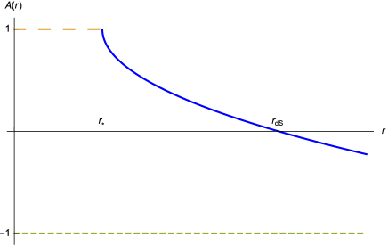
Figure 21: De Sitter-like geometry in an external space region $(r_{*}<r<\infty)$ with a de Sitter type horizon at $r_{\rm dS}$, and with one finite-extent internal forbidden region $(0<r<r_{*})$.

       (i) When $P^{\prime}_{4}(r_{*})>0$ the forbidden region (for de Sitter asymptotics – lower sign in (40)) is a finite-extent internal one $(0<r<r_{*})$ – see Fig.10 below where $(M>0,c_{1}\leavevmode\nobreak\ {\rm any},c_{0}<0)$ and Fig.21 below where $(M=0,c_{1}>0,c_{0}<0)$.

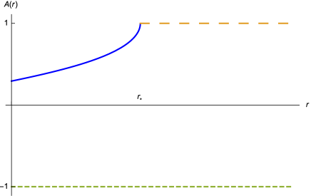
Figure 11: Finite-extent internal region of regular geometry $(0<r<r_{*})$, and one external infinite forbidden region $(r_{*}<r<\infty)$.

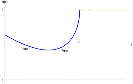
Figure 12: Black hole with two horizons of Reissner-Nordström-type at $r_{\rm RN1}$ and $r_{\rm RN2}$ within in a finite extent internal space region $(0<r<r_{*})$, and an infinite external forbidden region $(r_{*}<r<\infty)$.

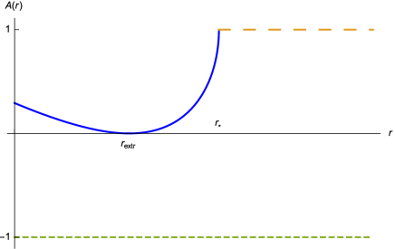
Figure 13: Extremal black hole with two coallescing horizons of Reissner-Nordström-type at $r_{\rm extr}$ within in a finite extent internal space region $(0<r<r_{*})$, and an infinite external forbidden region $(r_{*}<r<\infty)$.

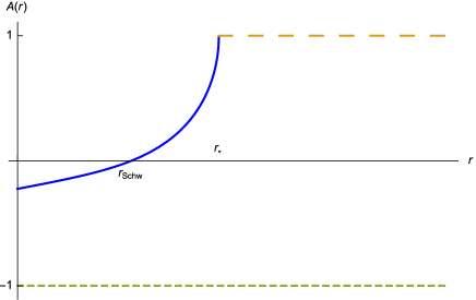
Figure 14: Black hole in a finite-extent internal space region $(0<r<r_{*}$ with a Schwarzschild-type horizon at $r_{\rm Schw}$, and with an infinite external forbidden region $(r_{*}<r<\infty)$.

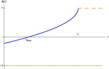
Figure 19: Black hole with a Schwarzschild-type horizon within a finite-extent internal space region $(0<r<r_{*})$, and with an infinite external forbidden region $(r_{*}<r<\infty)$.

       (ii) When $P^{\prime}_{4}(r_{*})<0$ the forbidden region (for de Sitter asymptotics) is an infinite-extent external one $(r_{*}<r<\infty)$ – see Figs.11,12,13,14 below where $(M<0,c_{1}\leavevmode\nobreak\ {\rm any},c_{0}>0)$, and Fig.19 below where $(M=0,c_{1}<0,c_{0}>1)$.

• Two simple positive roots $r_{1*}>0$ and $r_{2*}>0$ of $P_{4}(r)$, $r_{1*}<r_{2*}$, with two physical spacetime singularities there (cf. (40)-(42)).

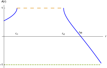
Figure 8: De Sitter-like geometry with one intermediate finite-extent forbidden region $(r_{1*}<r<r_{2*})$, and a de Sitter-type horizon at $r_{\rm dS})$.

       (i) For $P^{\prime}_{4}(r_{1*})<0$ and $P^{\prime}_{4}(r_{2*})>0$ the forbidden region (for de Sitter asymptotics) is a finite-extent intermediate one $(r_{1*}<r<r_{2*})$ – see Figs.8,9 below where $(M>0,c_{1}<-4M\bigl{(}c_{0}/3M\bigr{)}^{3/4},c_{0}>0)$.

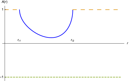
Figure 15: Finite-extent intermediate space region with regular geometry $(r_{1*}<r<r_{2*})$, and with two forbidden regions – one finite-extent internal $(0<r<r_{1*}$ and one infinite external $(r_{2*}<r<\infty)$.

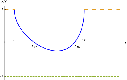
Figure 16: Blackhole with two horizons of Reissner-Nordström-type within a finite-extent intermediate space region $(r_{1*}<r<r_{2*})$, and with two forbidden regions – one finite-extent internal $(0<r<r_{1*}$ and one infinite external $(r_{2*}<r<\infty)$.

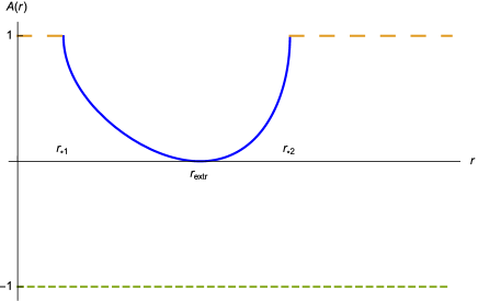
Figure 17: Extremal blackhole with two coallescing horizons of Reissner-Nordström-type within a finite-extent intermediate space region $(r_{1*}<r<r_{2*})$, and with two forbidden regions – one finite-extent internal $(0<r<r_{1*}$ and one infinite external $(r_{2*}<r<\infty)$.

       (ii) For $P^{\prime}_{4}(r_{1*})>0$ and $P^{\prime}_{4}(r_{2*})<0$ there are two forbidden regions (for de Sitter asymptotics): a finite-extent internal $(0<r<r_{1*})$ and an infinite-extent external $(r_{2*}<r<\infty)$. See Figs.15,16,17 below where $(M<0,c_{1}\leavevmode\nobreak\ {\rm any},c_{0}<0)$.

• Double positive root $r_{\rm DW}\equiv\bigl{(}c_{0}/3M\bigr{)}^{1/4}$ of $P_{4}(r)$:

  $$P_{4}(r)=(r-r_{\rm DW})^{2}M\bigl{[}6r^{2}_{\rm DW}+4r_{\rm DW}(r-r_{\rm DW})+(r-r_{\rm DW})^{2}\bigr{]}$$ (43)

  yield spacetime geometry (17) with:

  $$A(r)=1\pm|r-r_{\rm DW}|\sqrt{M\bigl{[}6r^{2}_{\rm DW}+4r_{\rm DW}(r-r_{\rm DW})+(r-r_{\rm DW})^{2}\bigr{]}}$$ (44)

  which contains a domain wall located at $r=r_{\rm DW}\equiv\bigl{(}c_{0}/3M\bigr{)}^{1/4}$ (see Fig.2 and Fig.7 below where $(M>0,c_{1}=-4M\bigl{(}c_{0}/3M\bigr{)}^{3/4},c_{0}<0)$) since while $A(r)$ is continuous there, its derivative $\partial_{r}A$ has a discontinuity. Therefore, the second derivative gets a delta-function contribution plus an additional discontinuity at $r=r_{\rm DW}\equiv\bigl{(}c_{0}/3M\bigr{)}^{1/4}$:

  $$\partial_{r}^{2}A=-\sqrt{24M}r_{\rm DW}\delta(r-r_{\rm DW})-\sqrt{\frac{8M}{3}}{\rm sign}(r-r_{\rm DW})+{\rm regular}\;.$$ (45)

  Eq.(45) through the SSS Einstein equation (23) and Eq.(28) indicates the presence of a surface stress-energy tensor $S^{\mu}_{\nu}$ of an additional static charged thin-shell (brane) matter source located at $r=r_{\rm DW}\equiv\bigl{(}c_{0}/3M\bigr{)}^{1/4}$ so that (23) is modified as:

  $$L(F^{2})=24\chi M+\partial_{r}^{2}A+\frac{2}{r}\partial_{r}A-{T^{\theta}_{\theta}}\bigm{|}_{\rm brane}\;,$$ (46)

  $${T^{\mu}_{\nu}}\bigm{|}_{\rm brane}=S^{\mu}_{\nu}\delta(r-r_{\rm DW})\quad,\quad S^{0}_{0}=S^{r}_{r}=0\;\;,\;\;S^{\theta}_{\theta}=S^{\phi}_{\phi}\;,$$ (47)

  whereas (26) is modified as:

  $$F_{0r}L^{\prime}(F^{2})=\frac{q}{16\pi\,r^{2}}+\frac{1}{8}j^{0}_{\rm brane}{\rm sign}(r-r_{\rm DW})\;,$$ (48)

  with $j^{0}_{\rm brane}$ being the surface brane charge density. Relations (47) comply with the general formalism for thin-shell domain walls developed in Ref.[34].

  Similarly, there appear the same brane stress-energy and surface charge contributions in the modification of (28):

  $$F_{0r}\Bigl{[}\frac{q}{16\pi\,r^{2}}+\frac{1}{2}j^{0}_{\rm brane}{\rm sign}(r-r_{\rm DW})\Bigr{]}$$

  $$=-\frac{4\pi\,r^{2}}{q}\Bigl{[}\partial_{r}^{2}A-\frac{2}{r^{2}}(A-1)-{T^{\theta}_{\theta}}\bigm{|}_{\rm brane}\Bigr{]}\;.$$ (49)

  Choosing the value of the brane pressure:

  $$S^{\theta}_{\theta}=-\sqrt{24M}r_{\rm DW}\;,$$ (50)

  we exactly cancell the delta-function part in $L(F^{2})$ (46) and $F_{0r}$ (49) due to the delta-function singularity in $\partial_{r}^{2}A$ (45), whereas the discontinuous term on the l.h.s. of (49) is matched by the discontinuity in $\partial_{r}^{2}A$ (45). Let us note that Eq.(50) together with (47) implies that the thin-shell matter forming the domain wall is an exotic matter (violating null energy condition).

• Another class of SSS solutions for $A(r)$ with de Sitter-like asymptotics is when $P_{4}(r)>1$ for all $r$, i.e., $A(r)=1-\sqrt{P_{4}(r)}<0$ for all $r$, which means that $r$ becomes timelike whereas $t\equiv z$ becomes “radial-like” spacelike. In this case the SSS metric (17) acquires the following form upon introducing a new “cosmological” time coordinate $\xi$ instead of the timelike $r$:

  $$ds^{2}=-d\xi^{2}+|A\bigl{(}r(\xi)\bigr{)}|dz^{2}+r^{2}(\xi)\bigl{(}d\theta^{2}+\sin^{2}\theta d\phi^{2}\bigr{)}\;\;,\;\;\frac{dr}{d\xi}=\sqrt{|A\bigl{(}r(\xi)\bigr{)}|}\;,$$ (51)

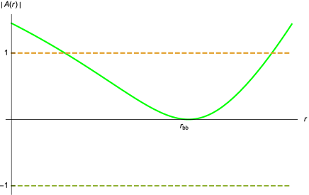
Figure 5: Kantowski-Sachs universe: the left branch describing a contracting universe with a big crunch on the interval $(0<r<r_{\rm b})$, and the right branch describing an expanding universe with a big bang on the interval $(r_{\rm b}<r<\infty)$; $r$ is timelike coordinate.

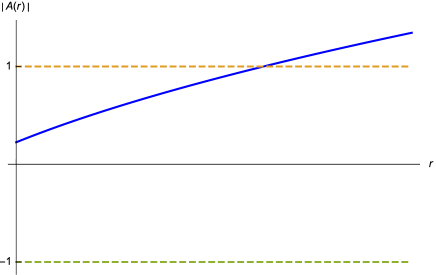
Figure 18: Kantowski-Sachs slowly expanding universe.

  This describes the geometry of a particular type of Kantowski-Sachs universe [35] – contracting, expanding or bouncing – depending of the values of the free integration constants. See Figs.3,4,5 below where $(M>0,c_{1}\geq-4M\bigl{(}c_{0}/3M\bigr{)}^{3/4},c_{0}>1)$ and Fig.18 below where $(M=0,c_{1}>0,c_{0}>1)$.

On the other hand, for de Sitter-like asymptotics (lower sign in (19)) there might exist one or two horizons $r_{0}$ of $A(r)$ provided there are (one or two) positive roots $r_{0}$ of the related polynomial $Q_{4}(r)$:

$$Q_{4}(r)\equiv P_{4}(r)-1=Mr^{4}+c_{1}r+c_{0}-1\;,$$ (52)

$$Q_{4}(r_{0})=0\;\;\to\;\;A(r_{0})=1-\sqrt{1+Q_{4}(r_{0})}=0\;.$$ (53)

The various types of horizons are as follows. For one positive root $r_{0}$ of $Q_{4}(r)\equiv P_{4}(r)-1$ (52)-(53):

• The single horizon $r_{0}\equiv r_{\rm Schw}$ is of Schwarzschild type (see Fig.14 below where $(M<0,c_{1}\leavevmode\nobreak\ {\rm any},C_{0}>1)$, and Fig.19 below where $(M=0,c_{1}<0,c_{0}>1)$) for:

  $$A(r_{0})=0\quad,\quad\partial_{r}A(r_{0})=-\frac{1}{2}P^{\prime}_{4}(r_{0})>0\;;$$ (54)

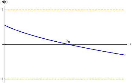
Figure 20: De Sitter-like geometry with a de-Sitter type horizon at $r_{\rm dS}$.

• The single horizon $r_{0}\equiv r_{\rm dS}$ is of de Sitter type (see Figs.1,2,8,10,20,21 below where ) for:

  $$A(r_{0})=0\quad,\quad\partial_{r}A(r_{0})=-\frac{1}{2}P^{\prime}_{4}(r_{0})<0\;.$$ (55)

For two positive roots $r^{(1)}_{0}<r^{(2)}_{0}$ of $Q_{4}(r)\equiv P_{4}(r)-1$ (52)-(53):

• The two horizons are of the same type as for the Schwarzschild-de Sitter black hole when:

  $$A(r^{(1,2)}_{0})=0\quad,\;\;\partial_{r}A(r^{(1)}_{0})>0\;\;,\;\;\partial_{r}A(r^{(2)}_{0})<0\;,$$

  $${\rm i.e.}\quad P^{\prime}_{4}(r^{(1)}_{0})<0\quad,\quad P^{\prime}_{4}(r^{(2)}_{0})>0\;,$$ (56)

  (see Figs.6,7 below where $\bigl{(}M>0,-4M\Bigl{(}\frac{c_{0}}{3M}\Bigr{)}^{3/4}\leq c_{1}<-4M\Bigl{(}\frac{c_{0}-1}{3M}\Bigr{)}^{3/4},c_{0}>1\bigr{)}$ ). In the case $\bigl{(}M>0,c_{1}<-4M\Bigl{(}\frac{c_{0}}{3M}\Bigr{)}^{3/4},c_{0}>1\bigr{)}$ (see Fig.9 below) there are again two horizons of the same type as for the Schwarzschild-de Sitter black hole, however they are separated by an intermediate forbidden region.

• The two horizons are of the same type as for the Reissner-Nordström black hole for:

  $$A(r^{(1,2)}_{0})=0\quad,\;\;\partial_{r}A(r^{(1)}_{0})<0\;\;,\;\;\partial_{r}A(r^{(2)}_{0})>0\;,$$

  $${\rm i.e.}\;\;P^{\prime}_{4}(r^{(1)}_{0})>0\quad,\quad P^{\prime}_{4}(r^{(2)}_{0})<0\;,$$ (57)

  however, in this case the black hole exists only in a finite-extent space region (see Fig.12 and Fig.16 where $\bigl{(}M<0,c_{1}>4|M|\Bigl{(}\frac{1-c_{0}}{3|M|}\Bigr{)}^{3/4},c_{0}<1\bigr{)}$).

• In the case of coallecense of the two roots of $A(r)$:

  $$A(r^{(1,2)}_{0})=0\;\;,\;\;r^{(1)}=r^{(2)}\;,\quad\partial_{r}A(r^{(1,2)}_{0})=0\;\;,\;{\rm i.e.}\;P^{\prime}_{4}(r^{(1,2)}_{0})=0\;,$$ (58)

  the horizon is of extremal black hole type (see Fig.13 and Fig.17 where $\bigl{(}M<0,c_{1}=4|M|\Bigl{(}\frac{1-c_{0}}{3|M|}\Bigr{)}^{3/4},c_{0}<1\bigr{)}$).

5 Graphical Representations of the Class of SSS Solutions of Modified ${\mathbf{D=4}}$ Gauss-Bonnet Gravity

In what follows we will graphically illustrate the various possible classes of solutions for $A(r)$ (19), focusing on de Sitter-like asymptotics of the latter, with or without physical singularities, including with or without domain walls, as well a with or without horizons (black hole type or de Sitter cosmological type) depending on the values of the free integration constants $(M,c_{1},c_{0})$.

5.1 Metrics Without Forbidden Regions ($\mathbf{M>0}$)

5.1.1 $\mathbf{\bigl{(}M>0,0<c_{0}<1,c_{1}>-4M(c_{0}/3M)^{3/4}\bigr{)}}$

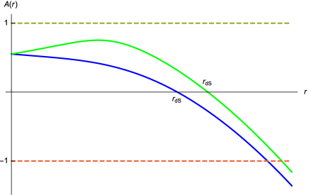
Figure 1: De Sitter-like (deviation from the standard de Sitter) $A(r)$ with a de Sitter-type horizon at $r_{\rm dS}$. The lower curve corresponds to $c_{1}>0$ and the upper curve corresponds to $-4M(c_{0}/3M)^{3/4}<c_{1}<0$.

5.1.2 $\mathbf{\bigl{(}M>0,0<c_{0}<1,c_{1}=-4M(c_{0}/3M)^{3/4}\bigr{)}}$

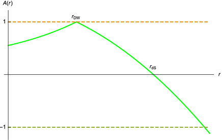
Figure 2: de Sitter-like $A(r)$ with a domain wall at $r=r_{\rm DW}\equiv\bigl{(}\frac{c_{0}}{3M}\bigr{)}^{1/4}$ and a de Sitter-type horizon at $r_{\rm dS}$. As pointed out above after Eq.(50) the thin-shell matter of the domain wall must be exotic.

5.1.3 $\mathbf{\bigl{(}M>0,c_{0}>1,c_{1}>0\bigr{)}}$

In this case $A(r)=1-\sqrt{P_{4}(r)}<0$ for all $r$, so the metric is given by (51), where the solution of $dr/d\xi=\sqrt{|A\bigl{(}r(\xi)\bigr{)}|}$ is $r(\xi)\simeq\sqrt{\sqrt{c_{0}}-1}\,\xi$ for small $\xi$, and $r(\xi)\simeq\exp\{M^{1/4}\xi\}$ for large $\xi$, and thus (51) describes monotonically expanding Kantowski-Sachs universe.

Figure 3: Monotonically expanding Kantowski-Sachs universe; $r$ is timelike coordinate.

5.1.4 $\mathbf{\bigl{(}M>0,c_{0}>1,0>c_{1}>-4M\bigl{(}(c_{0}-1)/3M\bigr{)}^{3/4}\bigr{)}}$

Here again $A(r)=1-\sqrt{P_{4}(r)}<0$ for all $r$, but now there is a local minimum of $|A(r)|$ at:

$$r=r_{\rm b}\equiv\bigl{(}\frac{|c_{1}|}{4M}\bigr{)}^{1/3}\;,$$ (59)

as depicted on Fig.4. Therefore, the metric (51) describes a bouncing Kantowski-Sachs universe.

Figure 4: Bouncing Kantowski-Sachs universe at $r=r_{\rm b}$; $r$ is timelike coordinate.

Namely, the size squared $|A\bigl{(}r(\xi)\bigr{)}|$ of the new radial dimension $z$ in (51) starts at a finite value $|A(0)|=\sqrt{\sqrt{c_{0}}-1}$ for $\xi=0$, drops down to a minimum value $|A(r_{\rm b})|$ at some finite cosmological time $\xi_{\rm b}$ and then it expands indefinitely for $\xi>\xi_{\rm b}$.

5.1.5 $\mathbf{\bigl{(}M>0,c_{0}>1,c_{1}=-4M\bigl{(}(c_{0}-1)/3M\bigr{)}^{3/4}\bigr{)}}$

This is a limiting case of the above bouncing Kantowski-Sachs solution, where now the minimum of the scale factor squared $|A(r)|$ vanishes when $r$ reaches $r_{\rm b}$:

$$|A(r_{\rm b})|=0\quad,\quad r_{\rm b}\equiv\bigl{(}\frac{c_{0}-1}{3M}\bigr{)}^{1/4}\;.$$ (60)

Accordingly we have a a very different properies of the pertinent Kantowski-Sachs universe.

In the present case the solution $r(\xi)$ of the second Eq.(51) splits into two branches:

• (a) Contracting Kantowski-Sachs universe with a big crunch on the interval $0\leq r\leq r_{\rm b}$:

  $$r(\xi)\simeq\left\{\begin{array}[]{ll}{\sqrt{|A(0)|}\,\xi}&\quad{\xi\sim 0\;,\;r\sim 0}\\ {r_{\rm b}-e^{-3Mr^{2}_{\rm b}\,\xi}}&\quad{\xi\to\infty\;,\;r\sim r_{\rm b}}\end{array}\right.$$ (63)

  Here the evolution starts at cosmological time $\xi=0$ with a non-zero scale factor squared $|A(0)|=\sqrt{\sqrt{c_{0}}-1}$ (“emergent universe”) and monotonically contracts to a big crunch $|A\bigl{(}r(\xi)\bigr{)}|\to|A(r_{\rm b})|=0$ at $\xi\to\infty$.

• (b) Expanding Kantowski-Sachs universe with a big bang on the interval $r_{\rm b}\leq r<\infty$:

  $$r(\xi)\simeq\left\{\begin{array}[]{ll}{r_{\rm b}+e^{3Mr^{2}_{\rm b}\,\xi}}&\quad{\xi\to-\infty\;,\;r\sim r_{\rm b}}\\ {e^{M^{1/4}\,\xi}}&\quad{\xi\to\infty\;,\;r\to\infty}\end{array}\right.$$ (66)

  Here evolution starts with a big bang at $\xi\to-\infty$ where the scale factor squared $|A\bigl{(}r(\xi)\bigr{)}|\to|A(r_{\rm b})|=0$ and then monotonically expands indefinitely for $\xi\to+\infty$.

5.1.6 $\mathbf{\bigl{(}M>0,c_{0}>1,-4M\bigl{(}(c_{0}-1)/3M\bigr{)}^{3/4}\bigr{)}>c_{1}>-4M\bigl{(}c_{0}/3M\bigr{)}^{3/4}\bigr{)}}$

Figure 6: Blackhole with two horizons – internal Schwarzschild-type at $r_{\rm Schw}$ and external de Sitter-type at $r_{\rm dS}$. Unlike the standard Schwarzschild-de Sitter blackhole here $A(r)$ is finite at $r=0$ ($A(0)=-(\sqrt{c_{0}}-1)$).

5.1.7 $\mathbf{\bigl{(}M>0,c_{0}>1,c_{1}=-4M\bigl{(}c_{0}/3M\bigr{)}^{3/4}\bigr{)}}$

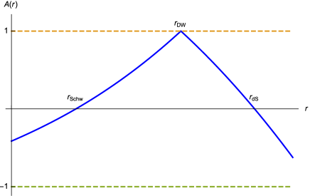
Figure 7: Blackhole with two horizons – internal Schwarzschild-type at $r_{\rm Schw}$ and external de Sitter-type at $r_{\rm dS}$, and with an additional domain wall at $r_{\rm DW}\equiv(c_{0}/3M)^{1/4}$ between the two horizons. As in subsubsection 5.1.2, in particular, an additional thin-shell brane exotic matter source must be present to match the delta-function singularities in the corresponding Einstein equations at $r=r_{\rm DW}$.

5.2 Metrics With One Forbidden Region ($\mathbf{M>0}$)

5.2.1 $\mathbf{\bigl{(}M>0,0<c_{0}<1,c_{1}<-4M\bigl{(}c_{0}/3M\bigr{)}^{3/4}\bigr{)}}$

5.2.2 $\mathbf{\bigl{(}M>0,c_{0}>1,c_{1}<-4M\bigl{(}c_{0}/3M\bigr{)}^{3/4}\bigr{)}}$

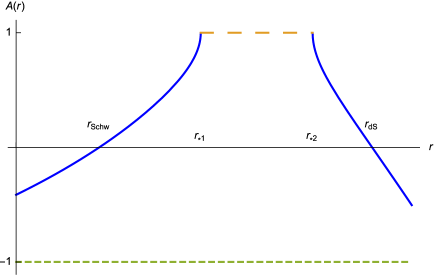
Figure 9: Black Hole with two horizons – a Schwarzschild-type at $r_{\rm Schw}$ and a de Sitter-type at $r_{\rm dS}$ separated by an intermediate finite-extent forbidden region $(r_{1*}<r<r_{2*})$.

5.2.3 $\mathbf{\bigl{(}M>0,c_{0}<0,c_{1}\;{\rm any}\bigr{)}}$

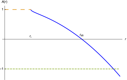
Figure 10: De Sitter-like geometry with a de Sitter-type horizon at $r_{\rm dS}$, and one internal finite-extent forbidden region $(0<r<r_{*})$.

5.3 Metrics With One Forbidden Region ($\mathbf{M<0}$)

5.3.1 $\mathbf{\bigl{(}M<0,0<c_{0}<1,c_{1}<4|M|\bigl{(}(1-c_{0})/3|M|\bigr{)}^{3/4}\bigr{)}}$

5.3.2 $\mathbf{\bigl{(}M<0,0<c_{0}<1,c_{1}>4|M|\bigl{(}(1-c_{0})/3|M|\bigr{)}^{3/4}\bigr{)}}$

5.3.3 $\mathbf{\bigl{(}M<0,0<c_{0}<1,c_{1}=4|M|\bigl{(}(1-c_{0})/3|M|\bigr{)}^{3/4}\bigr{)}}$

5.3.4 $\mathbf{\bigl{(}M<0,c_{0}>1,c_{1}\;{\rm any}\bigr{)}}$

5.4 Metrics With Two Forbidden Regions ($\mathbf{M<0}$)

5.4.1 $\mathbf{\bigl{(}M<0,c_{0}<0,c_{1}<4|M|\bigl{(}(1+|c_{0}|)/3|M|\bigr{)}^{3/4}\bigr{)}}$

5.4.2 $\mathbf{\bigl{(}M<0,c_{0}<0,c_{1}>4|M|\bigl{(}(1+|c_{0}|)/3|M|\bigr{)}^{3/4}\bigr{)}}$

5.4.3 $\mathbf{\bigl{(}M<0,c_{0}<0,c_{1}=4|M|\bigl{(}(1+|c_{0}|)/3|M|\bigr{)}^{3/4}\bigr{)}}$

5.5 Metrics with $\mathbf{M=0}$

5.5.1 $\mathbf{\bigl{(}M=0,c_{0}>1,c_{1}>0\bigr{)}}$

Here again $A(r)=1-\sqrt{P_{4}(r)}<0$ for all $r$ and the metric (51) describes in this case a slowly expanding Kantowski-Sachs universe: $|A\bigl{(}r(\xi)\bigr{)}|\sim\xi^{2/3}$ for $\xi\to\infty$.

5.5.2 $\mathbf{\bigl{(}M=0,c_{0}>1,c_{1}<0\bigr{)}}$

5.5.3 $\mathbf{\bigl{(}M=0,0<c_{0}<1,c_{1}>0\bigr{)}}$

5.5.4 $\mathbf{\bigl{(}M=0,c_{0}<0,c_{1}>0\bigr{)}}$

6 Avoiding Spacetime Singularities via Domain Walls

Let us consider two SSS solutions (19) with forbidden regions:

       (a) The one depicted on Fig.9 – describing black hole with two horizons (one Schwarzschild-type and one de Sitter-type) separated by an intermediate finite-extent forbidden region $(r_{*1}<r<r_{*2})$, where $r_{*1,2}$ are two roots of of the 4th-order polynomial under the square root in::

$$A_{1}(r)=1-\sqrt{Mr^{4}+c_{1}^{(1)}r+c_{0}^{(1)}}\;,$$ (67)

$$\bigl{(}M>0,c_{0}^{(1)}>1,c_{1}^{(1)}<-4M(c_{0}/3M)^{3/4}\bigr{)}\;.$$

       (b) The second one graphically depicted on Fig.10 – describing de Sitter-like geometry with a de Sitter-type horizon, and with one internal finite-extent forbidden region $(0<r<r_{*})$, where $r_{*}$ is a root of the 4th-order polynomial under the square root in:

$$A_{2}(r)=1-\sqrt{Mr^{4}+c_{1}^{(2)}r+c_{0}^{(2)}}\quad,\;\;\bigl{(}M>0,c_{0}^{(2)}<0,c_{1}^{(2)}\leavevmode\nobreak\ {\rm any}\bigr{)}\;.$$ (68)

Now, we can construct another SSS solution ${\widehat{A}}(r)$ without any spacetime singularities by picking a point $r={\widehat{r}}$ with ${\widehat{r}}<r_{1*}$ ($r_{1*}$ from (68)) and ${\widehat{r}}>r_{*}$ ($r_{*}$ from (67)), and glue together $A_{1}(r)$ and $A_{2}(r)$ at $r={\widehat{r}}$:

$${\widehat{A}}(r)=\left\{\begin{array}[]{ll}A_{1}(r)\;\;,&\quad 0<r\leq{\widehat{r}}\\ A_{2}(r)\;\;,&\quad{\widehat{r}}\leq r<\infty\end{array}\right.\;,$$ (71)

so that ${\widehat{A}}(r)$ is continuous at $r={\widehat{r}}$:

$$A_{1}({\widehat{r}})=A_{2}({\widehat{r}})\;\;\longrightarrow\;\;{\widehat{r}}=\frac{c_{0}^{(1)}-c_{0}^{(2)}}{c_{1}^{(2)}-c_{1}^{(1)}}\;,$$ (72)

but its first derivative has a discontinuity at $r={\widehat{r}}$:

$$\bigl{[}\partial_{r}{\widehat{A}}\bigr{]}_{{\widehat{r}}}\equiv\partial_{r}A_{2}({\widehat{r}})-\partial_{r}A_{1}({\widehat{r}})=-\frac{c_{1}^{(2)}-c_{1}^{(1)}}{2\sqrt{M{\widehat{r}}^{4}+c_{1}^{(2)}{\widehat{r}}+c_{0}^{(2)}}}\;,$$ (73)

and thus the second derivative acquires delta-function contribution at $r={\widehat{r}}$:

$$\partial_{r}^{2}{\widehat{A}}=\bigl{[}\partial_{r}{\widehat{A}}\bigr{]}_{{\widehat{r}}}\delta(r-{\widehat{r}})+\ldots\;.$$ (74)

As in the case of (45) above, Eq.(74) imply presence of thin-shell generated domain wall at $r={\widehat{r}}$ where the corresponding brane surface tension matching the delta-function term in (74) is (cf. (47) and (50)):

$$T^{\theta}_{\theta}=S^{\theta}_{\theta}\delta(r-{\widehat{r}})\quad,\quad S^{\theta}_{\theta}=\bigl{[}\partial_{r}{\widehat{A}}\bigr{]}_{{\widehat{r}}}\;,$$ (75)

with $\bigl{[}\partial_{r}{\widehat{A}}\bigr{]}_{{\widehat{r}}}$ as defined in (73). Note that the latter is negative, therefore so is the brane surface tension $S^{\theta}_{\theta}$, which confirms the exotic nature of the domain wall brane matter, as already pointed out above after Eq.(50).

The graphical representation of (71) (Fig.22) is completely analogous to the case of Fig.7 above where $\bigl{(}M>0,c_{0}>1,c_{1}=-4M(c_{0}/3M)^{3/4}\bigr{)}$.

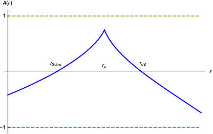
Figure 22: Blackhole with two horizons – internal Schwarzschild-type at $r_{\rm Schw}$ and external de Sitter-type at $r_{\rm dS}$, and with an additional domain wall at ${\widehat{r}}$ between the two horizons. The section of the graphics for $0<r<{\widehat{r}}$ is as in Fig.9, whereas the section for ${\widehat{r}}<r<\infty$ is as in Fig.10. Both forbidden regions in Fig.9 and Fig.10 are avoided.

The above described “cut and glue together” procedure closely resembles the “cut and paste” formalism for constructing timelike thin-shell wormholes in Ref.[36], ch.15.

7 Discussion and Outlook

In the present paper we have studied in some detail the full class of static spherically symmetric (SSS) solutions in the recently proposed by us new modified Gauss-Bonnet gravity in $D=4$ based on the formalism of non-Riemannian spacetime volume-forms which avoids the need to couple the Gauss-Bonnet scalar to matter fields or to employ higher powers of the latter as in ordinary $D=4$ Einstein-Gauss-Bonnet gravity models, where the latter couplings are needed to avoid the ordinary $D=4$ Gauss-Bonnet density to become total derivative.

The dynamically triggered constancy of the Gauss-Bonnet density due to the equations of motion resulting from the non-Riemannian spacetime volume element by itself completely determines the solutions for the SSS metric component function $g_{00}=-A(r)$ parametrized by three free integration constants. Depending on the signs and values of the latter one finds SSS solutions with deformed (anti)-de Sitter geometry, black holes of Schwarzschild-de Sitter type, domain walls and Kantowski-Sachs universes (expanding, contracting and bouncing), as well as a multitude of SSS solutions exhibiting physical spacetime singularities not hidden behind horizons, which border finite-extent or infinitely large forbidden space regions.

According to the cosmic sensorship principle [37] the above class of SSS solutions with naked (visible) spacetime singularities should be ruled out as physically acceptible solutions. However, we showed that it is possible to avoid the singularities by inserting appropriate domain walls and pairwise matching solutions with singularities along the domain wall (a procedure analogous to the construction of timelike thin-shell wormholes in Ref.[36]).

In various cases the field-theoretic Lagrangian actions of the corresponding matter sources for the above SSS gravity solutions are identified – as a complicated nonlinear electrodynamics with a non-analytic functional dependence on $F^{2}$ (the square of the Maxwell tensor), and in a special case – as the $SO(3)$ nonlinear sigma model (the “hedgehog” scalar field [30]).

An important next task is to study SSS solutions in the more general setting when the composite field $\chi\equiv\frac{\Phi(C)}{\sqrt{-g}}$ (9) will not be “frozen” to a constant, i.e., when one needs to solve the full modified Einstein equations (10) with $\chi=\chi(r)$. Moreover, in the latter case we will need to consider the more general form of SSS metric than (17):

$$ds^{2}=-A(r)dt^{2}+B(r)dr^{2}+r^{2}\bigl{(}d\theta^{2}+\sin^{2}\theta d\phi^{2}\bigr{)}\quad,\;\;B(r)\neq A^{-1}(r)\;.$$ (76)

Inserting the more general SSS ansatz (76) into the system of Eqs.(10) and (15), one gets a very complicated coupled system of highly nonlinear ordinary differentional equations of second order which clearly will require numerical treatment.

References

- [1] S. Capozziello and M. De Laurentis, Phys. Reports 509, 167 (2011) (arXiv:1108.6266).
- [2] S. Capozziello and V. Faraoni, “Beyond Einstein Gravity – A Survey of Gravitational Theories for Cosmology and Astrophysics”, (Springer, 2011).
- [3] S. Nojiri and S. Odintsov, Phys. Reports 505, 59 (2011).
- [4] S. Nojiri, S. Odintsov and V. Oikonomou, Phys. Reports 692, 1 (2017) (arXiv:1705.11098).
- [5] E. Guendelman, E. Nissimov and S. Pacheva, Bulg. J. Phys. 41, 123 (2014) (arXiv:1404.4733).
- [6] E. Guendelman, E. Nissimov and S. Pacheva, Int. J. Mod. Phys. A30, 1550133 (2015) (arXiv:1504.01031).
- [7] E. Guendelman, Mod. Phys. Lett. A14, 1043-1052 (1999) (arXiv:gr-qc/9901017).
- [8] E. Guendelman and A. Kaganovich, Phys. Rev. D60, 065004 (1999) (arXiv:gr-qc/9905029).
- [9] E. Guendelman, E. Nissimov and S. Pacheva, Eur. J. Phys. C75, 472-479 (2015) (arXiv:1508.02008); Eur. J. Phys. C76, 90 (2016) (arXiv:1511.07071).
- [10] E. Guendelman, E. Nissimov and S. Pacheva, Int. J. Mod. Phys. D25, 1644008 (2016) (arXiv:1603.06231).
- [11] E. Guendelman, E. Nissimov and S. Pacheva, in “Quantum Theory and Symmetries with Lie Theory and Its Applications in Physics”, vol.2 ed. V. Dobrev, Springer Proceedings in Mathematics and Statistics v.225 (Springer, 2018).
- [12] E. Guendelman, E. Nissimov and S. Pacheva, arXiv:1808.03640, to be published in 10th Jubilee Conference of Balkan Physical Union, AIP Conference Proceedings.
- [13] E. Berti, E. Barausse, V. Cardoso et al., Class. Quantum Grav. 32, 243001 (2015) (arXiv:1501.07274).
- [14] L. Barack, V. Cardoso, S. Nissanke et al., arXiv:1806.05195, to appear in Class. Quant. Grav. (2018).
- [15] S. Nojiri and S. D. Odintsov, Phys. Lett. B631, 1 (2005) (hep-th/0508049).
- [16] S. Nojiri, S.D. Odintsov and O.G. Gorbunova, J. Physics A39, 6627 (2006) (arXiv:hep-th/0510183).
- [17] G. Cognola, E. Elizalde, S. Nojiri, S.D. Odintsov and S. Zerbini, Phys. Rev. D73, 084007 (2006) (arXiv:hep-th/0601008).
- [18] A. De Felice and S. Tsujikawa, Phys. Lett. B675, 1 (2009) (arXiv:0810.5712).
- [19] P.Kanti, R.Gannouji and N. Dadhich, Phys. Rev. D92, 041302 (2015) (arXiv:1503.01579); Phys. Rev. D92, 083524 (2015) (arXiv:1506.04667).
- [20] L. Sberna and P. Pani, Phys. Rev. D96, 124022 (2017) (arXiv:170806371).
- [21] M. Heydari-Fard, H. Razmi and M. Yousefi, Int. J. Mod. Phys. D26, 1750008 (2017).
- [22] S.Carloni and J.Mimoso Eur. Phys. J. C77, 547 (2017).
- [23] M. Benetti, S. Santos da Costa, S. Capozziello, J. S. Alcaniz and M. De Laurentis, Int. J. Mod. Phys. D27, 1850084 (2018) (arXiv:1803.00895.
- [24] S.Odintsov, V.Oikonomou and S. Banerjee, arXiv:1807.00335.
- [25] E. Guendelman, E. Nissimov and S. Pacheva, arXiv:1809.00321.
- [26] R. Myrzakulov, L. Sebastiani and S. Zerbini, Gen. Rel. Gravit. 45, 675 (2013) (arXiv:1208.3392).
- [27] P. Bargue and E. Vagenas, Eur. Phys. Lett. 115, 60002 (2016) (arXiv:1609.07933).
- [28] I. Radinschi, T. Grammenos, F. Rahaman, A. Spanou, M. Cazacu, S. Chattapadhyay and A. Pasqua, arXiv:1807.00300, to appear in Advances in High Energy Physics.
- [29] T. Torii and H. Maeda, Phys. Rev. D72, 064007 (2005) (hep-th/0504141).
- [30] E. Guendelman and A. Rabinowitz, Phys. Rev. D44, 3152-3158 (1991).
- [31] K. Bronnikov, Phys. Rev. D63, 044005 (2001) (arXiv:gr-qc/0006014).
- [32] I. Dymnikova, Class. Quantum Grav. 21, 4417-29 (2004) (textslgr-qc/0407072).
- [33] A. Einstein and N. Rosen, Phys. Rev. 48, 73-77.
- [34] S. Blau, E. Guendelman and A. Guth, Phys. Rev. D35, 1747-1766 (1987).
- [35] R. Kantowski and R. Sachs, J. Math. Phys. 7, 443 (1966).
- [36] M. Visser, “Lorentzian Womholes”, Springer (1996).
- [37] R. Penrose, Riv. Nuovo Cim. 1, 252-276 (1969)..