Mapping the QCD phase diagram with statistics friendly distributions

Abstract

We demonstrate that the multiplicity distribution of a system located in the vicinity of a first-order phase transition can be successfully measured in terms of its factorial cumulants with a surprisingly small number of events. This finding has direct implications for the experimental search of a QCD phase transition conjectured to be located in the high baryon density region of the QCD phase diagram.

One of the key questions of the physics of strong interactions is the possible existence of a first-order phase transition accompanied by a critical point. While lattice QCD has established that the transition at vanishing net-baryon density is an analytic cross over Aoki et al. (2006), the presence of a first-order transition accompanied by a critical point has been conjectured based on many model calculations (see e.g. Stephanov (2004); Bzdak et al. (2019) for a review). To search for such a possible transition in experiment, fluctuations of conserved charges in relativistic heavy ion collisions have been considered as promising probes Jeon and Koch (2000); Asakawa et al. (2000); Stephanov (2009); Skokov et al. (2011); Stephanov (2011); Luo et al. (2012); Luo and Xu (2017); Herold et al. (2016); Zhou et al. (2012); Wang and Yang (2012); Karsch and Redlich (2011); Schaefer and Wagner (2012); Chen et al. (2011); Fu et al. (2010); Cheng et al. (2009). Special attention has been paid to the cumulants of the net-baryon or net-proton number distribution as they are particularly sensitive to the details of the transition from hadron gas to quark-gluon plasma in the cross-over region Skokov et al. (2011); Karsch and Redlich (2011) as well as near a potential critical point Stephanov (2009). This sensitivity is expected to increase with the order of the cumulant Stephanov (2009), the measurement of which is commonly believed to require increasing statistics.

In this paper we show, quite generally, that it requires surprisingly few events to determine if a system is located close to a first-order phase transition. This finding has direct implications on the search for the QCD phase transition, but will also be relevant for any other (mesoscopic) systems where fluctuation measurements are meaningful. It is well known that the multiplicity distribution of a system close to a first-order phase transition is a two-component or bi-modal distribution reflecting the two (dense and dilute) phases. If the system is right at the transition it has two maxima of equal magnitude, reflecting the equal probability of the two phases. As one moves away from the transition, one of the maxima becomes smaller, reflecting the fact that away from the transition one phase is much more probable than the other. Thus, for small systems and not too far from the transition, the presence of the other phase still shows up in the multiplicity distribution (for a detailed discussion, see Bzdak et al. (2018)). As discussed in Bzdak et al. (2018), such a two-component multiplicity distribution, even in the case when one of the components is rather small, has a very characteristic behavior of its factorial cumulants: with increasing order they increase rapidly in magnitude with alternating sign (in contrast, ultrarelativistic quantum molecular dymamics (UrQMD) calculations give higher order factorial cumulants consistent with zero He and Luo (2017)). This characteristic may be used to establish the existence of a two-component multiplicity distribution, which in turn would provide strong evidence that the system is close to a first-order phase transition.

Such a characterization requires factorial cumulants of many orders that are commonly believed to require large statistics. However, as we show, the two-component distributions relevant for a first-order phase transition are remarkably statistics friendly in the sense that for a given and rather limited number of events factorial cumulants can be reliably extracted to a surprisingly high order. Surprisingly, this is even the case if the second mode (component) is rather tiny and is difficult to see directly in the multiplicity distribution. This finding, therefore, demonstrates that a search for a first-order phase transition via fluctuation measurements is practically feasible and does not require unrealistic levels of statistics.

In the following we illustrate our findings in the context of preliminary results of the STAR Collaboration. However, our arguments are quite general and are not restricted to the QCD phase transition. The preliminary results from the STAR Collaboration for the ratio of fourth-order over second-order (net)-proton cumulants show an intriguing pattern Luo (2015a). It grows rapidly with decreasing beam energy from $\sqrt{s}=19.6$ GeV reaching a large value at $7.7$ GeV. It was argued Bzdak et al. (2017) that this behavior is caused by a strong increase of multi-proton correlations with decreasing energy. In addition it was found Bzdak et al. (2018), that at the lowest energy, $\sqrt{s}=7.7{\rm\,GeV}$, where the deviation of the cumulants from a Poisson baseline (or rather binomial due to baryon conservation) are the largest, the first four (factorial) cumulants, so far measured by STAR, are consistent with a two-component proton multiplicity distribution, albeit with the second component being rather small. Of course the first four cumulants are not enough to sufficiently constrain the multiplicity distribution. Therefore, it is essential to measure (factorial) cumulants of higher order to either confirm or rule out that the underlying distribution is indeed a two-component one consistent with a first-order phase transition. As we show this is possible due to the “statistics friendly” properties of these two-component distributions even for the very limited statistics of the present STAR data set.

Specifically, in this paper we study various proton multiplicity distributions to evaluate the statistical errors of higher order factorial cumulants. In our studies we choose a rather small number of events, approximately 150000 (144393 to be more precise XL- (2018)), which is the statistics underlying the STAR measurement for the most central Au+Au collisions at $\sqrt{s}=7.7$ GeV at RHIC Adamczyk et al. (2014); Luo (2015a). We will only consider multiplicity distributions of one species of particles, which are protons in our case.

To evaluate the statistical errors numerically, we sample the number of protons, $N$, $n_{\rm events}=144393$ times from a given multiplicity distribution $P(N)$. We then calculate the cumulants, $K_{n}$ and the factorial cumulants $C_{n}$ for $n=2,...,9$. Next we repeat this sampling $n_{\rm run}$ times, where $n_{\rm run}$ is sufficiently large so that the results presented below do not depend on $n_{\rm run}$. This procedure then gives us $n_{\rm run}$ “measurements” or samples of $K_{n}$ and $C_{n}$, $\{K^{(1)}_{n},\ldots,K^{(n_{\rm run})}_{n}\}$ and $\{C^{(1)}_{n},\ldots,C^{(n_{\rm run})}_{n}\}$.

From these samples we calculate the variance, for example, in the case of the factorial cumulants $C_{n}$ we have

$$\mathrm{Var}\left(C_{n}\right)=\frac{1}{n_{\mathrm{run}}}\sum_{i=1}^{n_{\mathrm{run}}}\left(C_{n}^{(i)}\right)^{2}-\left(\frac{1}{n_{\mathrm{run}}}\sum_{i=1}^{n_{\mathrm{run}}}C_{n}^{(i)}\right)^{2}.$$ (1)

The expected absolute error, $\Delta C_{n}$, is then given by $\Delta C_{n}=\sqrt{\mathrm{Var}\left(C_{n}\right)}$, whereas the relative error is $\Delta C_{n}/C_{n}$, where $C_{n}$ denotes the true value directly calculated from the multiplicity distribution $P(N)$.

An alternative way to calculate the expected error is by means of the delta method (see, e.g., Davison (2003); Luo (2015b); Luo and Xu (2017) for details). In the case at hand, where we want to calculate the errors for (factorial) cumulants, application of the delta method is straightforward. Let us discuss this in more detail for the case of the factorial cumulant. The random variables are the moments about zero, $\mu_{k}=\left\langle N^{k}\right\rangle$. Therefore, we express the factorial cumulant, $C_{n}$, in terms of the moments, $C_{n}=F(\mu_{1},\ldots,\mu_{n})$. Then according to the delta method the variance of $C_{n}$ for a sample with $n_{\rm events}$ events is given by

$$\mathrm{Var}\left(C_{n}\right) = \sum_{i=1}^{n}\sum_{j=1}^{n}\frac{\partial F}{\partial\mu_{i}}\frac{\partial F}{\partial\mu_{j}}\mathrm{Cov}\left(\mu_{i},\mu_{j}\right),$$ (2)

$$\mathrm{Cov}(\mu_{i},\mu_{j}) = \frac{1}{n_{\mathrm{events}}}\left(\mu_{i+j}-\mu_{i}\mu_{j}\right).$$ (3)

The absolute error is then again given by $\Delta C_{n}=\sqrt{\mathrm{Var}\left(C_{n}\right)}$. For example, we obtain the following for the variance of $C_{2}$ (after re-expressing the moments $\mu_{i}$ in terms of factorial cumulants)

$$\mathrm{Var}\left(C_{2}\right)=\frac{1}{n_{\rm events}} \left[2\left(C_{1}+C_{2}\right)^{2}+2C_{2}+4C_{3}+C_{4}\right].$$ (4)

We find that the so obtained errors are in perfect agreement with those determined via the aforementioned numerical sampling method.

After having presented the methods for error determination let us turn to the results. The essential point of the present paper is the observation that a small deviation from Poisson or binomial distributions can result in rather peculiar distributions, which we call statistics friendly distributions. From these distributions one may obtain factorial cumulants of high orders with a rather limited number of events. One example is a simple two-component distribution discussed recently in Ref. Bzdak et al. (2018)

$$P(N)=(1-\alpha)P_{(a)}(N)+\alpha P_{(b)}(N),$$ (5)

where both $P_{(a)}$ and $P_{(b)}$ are the proton multiplicity distributions characterized by small or even vanishing factorial cumulants. This distribution not only serves as a nice example for a statistics friendly distribution, but also, as argued recently in Ref. Bzdak et al. (2018), such a distribution would be consistent with a system with a finite number of particles being close to a first-order phase transition. The analysis in Ref. Bzdak et al. (2018) found that $P(N)$ given by Eq. (5) with $\alpha\approx 0.0033$, $P_{(a)}(N)$ given by binomial ($B=350$, $p\approx 0.1144$) and $P_{(b)}(N)$ given by Poisson ($\langle N_{(b)}\rangle=25.3525$) is able to reproduce the preliminary results by the STAR Collaboration for the proton cumulants at $\sqrt{s}=7.7{\rm\,GeV}$ Luo (2015a). In addition it was found that the above distribution predicts factorial cumulants to roughly scale like $C_{n+1}/C_{n}\sim-15$, i.e., they alter in sign from order to order while increasing in absolute value by more than an order of magnitude. In other words, the small admixture of a Poisson distribution changes the factorial cumulants dramatically, from being close to zero to almost exponentially increasing in magnitude. The same dramatic difference can also be seen in the expected error for a finite sampling. This is shown in Fig. 1, where in panel (a) we show the histogram of $C_{n}^{(i)}/C_{n}$ from our numerical sampling (based on $n_{\rm events}=144393$ events) for the binomial distribution only, i.e., $P_{(a)}(N)$. For completeness we note that the analytical values of $C_{n}$ for binomial are given by $C_{n}=(-1)^{n+1}(n-1)!Bp^{n}$. The distribution gets very wide already for $C_{3}$. In contrast, in panel (b) of Fig. 1 we show equivalent histograms for the two-component distribution, Eq. (5). Again, the small admixture of a Poisson distribution changes the situation dramatically. In this case the distributions are so narrow that a measurement of even the 8-th order factorial cumulants may be feasible with as little as 150000 events.

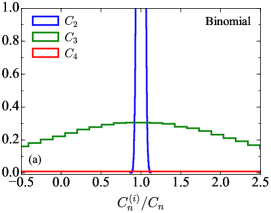
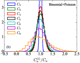
Figure 1: Histogram (normalized to unity) of the factorial cumulant, $C_{n}^{(i)}$, fluctuating from experiment to experiment, divided by a known (evaluated analytically) value, $C_{n}$, based on 144393 events sampled from (a) the binomial distribution ($B=350$, $p=0.114$, $\langle N\rangle=pB\approx 40$) and (b) a distribution given by Eq. (5) (see text for details). The statistical errors are given by the widths of the corresponding histograms. In the panel (a), the histograms’ order by the height at the maximum is (from largest to smallest) $C_{2}$, $C_{3}$, and $C_{4}$. In the panel (b) the order (from largest to smallest) is: $C_{2}$, $C_{4}$, $C_{5}$, $C_{3}$, $C_{6}$, $C_{7}$, and $C_{8}$.

This finding is quantified in Fig. 2, where we show the relative errors $\Delta C_{n}/C_{n}$ for various distributions again based on $n_{\rm events}=144393$ event. The relative error for both the binomial distribution and the negative binomial distribution (NBD) with $\langle N\rangle=40$ and $k=80$, increase essentially exponentially with increasing order of the factorial cumulant. Obviously all of these distributions are statistics hungry, and the measurement of higher order factorial cumulants with good accuracy requires very large statistics. For the two-component model, labeled “Binomial + Poisson”, on the other hand the relative errors remain very small even for $C_{9}$. The actual values for the relative errors are (0.036, 0.16, 0.13, 0.14, 0.18, 0.26, 0.42, 0.91) for $(\Delta C_{2}/C_{2},\ldots,\Delta C_{9}/C_{9})$.

We also show as “Binomial + Poisson + effi” the result one would obtain, if one takes a finite detection efficiency of $\epsilon=0.65$ into account, that is $\left\langle N_{(b)}\right\rangle=25.3525\times\epsilon$, $p=0.1144\times\epsilon$ so that $\left\langle N\right\rangle=40\times\epsilon$. Again, the relative error for the factorial cumulants remains small but larger than that in the case without efficiency. Here we have (0.056, 0.29, 0.27, 0.31, 0.41, 0.61, 1.06, 2.55) for $(\Delta C_{2}/C_{2},\ldots,\Delta C_{9}/C_{9})$. This also means that using the efficiency uncorrected STAR data one could try to measure the factorial cumulants up to the seventh order where $\Delta C_{7}/C_{7}=1\pm 0.61$.

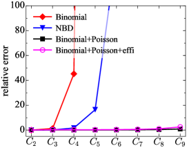
Figure 2: The relative error, $\Delta C_{n}/C_{n}$, of factorial cumulants for various proton multiplicity distributions based on 144393 events, as present in the most central $Au+Au$ collisions at RHIC. The binomial and negative binomial distributions presented here are statistically very demanding, whereas the distribution given by. Eq. (5) (Binomial+Poisson) with $\langle N\rangle=40$, allows to successfully measure higher order factorial cumulants with a relatively small number of events. This feature is also present for the efficiency uncorrected distribution (Binomial+Poisson+effi) where $\langle N\rangle=40\times 0.65$.

The above results may be understood qualitatively in the following way. In general we have two types of multiplicity distributions, $P(N)$. One where the higher order factorial cumulants are driven by the tails (Poisson, binomial, NBD etc.) and the other one where the higher order factorial cumulants are driven by some structure away from the tails. This is exactly the case of our model. To be a bit more precise the factorial cumulants of Eq. (5), assuming $\alpha\ll 1$ are given by

$$C_{n}\,\approx\,C_{n}^{(a)}+(-1)^{n}\alpha\mkern 1.5mu\overline{\mkern-1.5muN\mkern-1.5mu}\mkern 1.5mu^{n},$$ (6)

where $C_{n}^{(a)}$ is a factorial cumulant characterizing $P_{(a)}(N)$ and $\mkern 1.5mu\overline{\mkern-1.5muN\mkern-1.5mu}\mkern 1.5mu=\langle N_{(a)}\rangle-\langle N_{(b)}\rangle$. For $C_{n}^{(a)}$ being a Poisson or binomial the values of $C_{n}$ are completely dominated by the term $\alpha\mkern 1.5mu\overline{\mkern-1.5muN\mkern-1.5mu}\mkern 1.5mu^{n}$, which results in very large factorial cumulants. The error, $\Delta C_{n}$, on the other hand, is of the same magnitude as that of the first term, $\Delta C^{(a)}_{n}$ (in practice $\Delta C_{n}^{(a)}/\Delta C_{n}$ ranges from $\sim 0.95$ for $n=2$ to $\sim 0.2$ for $n=9$). Thus we have a situation, where the error of the factorial cumulant is of the same magnitude as that of a binomial distribution, but the factorial cumulant is orders of magnitude larger. Consequently, and not surprisingly, the relative error is much smaller for the two-component distribution than for the binomial distribution. It is worth noting that $C_{n}$ scales linearly with $\alpha$ and the two-component distribution is statistics friendly even if the second mode is tiny, i.e., $\alpha$ is small (provided $\mkern 1.5mu\overline{\mkern-1.5muN\mkern-1.5mu}\mkern 1.5mu^{n}$ is large enough).

Finally, we note that in the case of Eq. (5), the regular cumulnats are less statistics friendly. This is presented in Fig. 3. The reason for this is the same as just stated. The absolute errors for both cumulants and factorial cumulants are of the same magnitude, $\Delta K_{n}\sim\Delta C_{n}$. On the other hand, for the two-component model, the factorial cumulants are very large while the regular cumulants are only modestly larger than that of a simple binomial distribution. This is a result of the alternating signs of the factorial cumulants. For example, the sixth order cumulant, $K_{6}$, is given in terms of the factorial cumulants as $K_{6}=\langle N\rangle+31C_{2}+90C_{3}+65C_{4}+15C_{5}+C_{6}$ (see e.g., Ref. Bzdak et al. (2018)). For our example of ”binomial+Poisson+effi”, where we see a rapid increase in the relative error, we have $C_{6}\approx 3080$, $15C_{5}\approx-4600$ and $65C_{4}\approx 1970$. As a result, $K_{6}\approx 180\ll C_{6}$, and consequently the relative error is much larger for $K_{6}$ as compared to $C_{6}$.

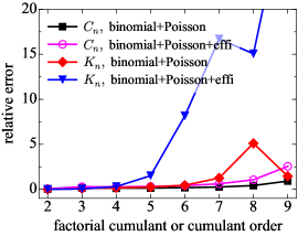
Figure 3: The relative errors of the factorial cumulants, $\Delta C_{n}/C_{n}$, and the regular cumulants, $\Delta K_{n}/K_{n}$, based on 144393 events sampled from a distribution given by Eq. (5).

In summary, we demonstrated that for the multiplicity distribution given by Eq. (5), which is relevant in the context of searching for structures in the QCD phase diagram, factorial cumulants of high orders can be determined with a relatively small number of events. This is in contrast to various statistics hungry distributions (Poisson, binomial, NBD, etc.), for which the error increases nearly exponentially with increasing order. As shown in Ref. Bzdak et al. (2018), the distribution, Eq. (5), describes the preliminary STAR data for proton cumulants (up to the forth order) in central Au+Au collisions at $\sqrt{s}=7.7{\rm\,GeV}$. Because this distribution is statistics friendly, it can be further tested by evaluating the higher order factorial cumulants even with the presently available STAR data set of $144393$ events for the most central collisions. We also pointed out that factorial cumulants are more statistics friendly when compared to regular cumulants, which, in the case of Eq. (5), results from a delicate cancellation of large factorial cumulants. Assuming that $C_{4}=170$ (as extracted from preliminary STAR data) we predict:

$$C_{5} = -307\,(1\pm 0.31),\quad C_{6}=3085\,(1\pm 0.41),$$

$$C_{7} = -30155\,(1\pm 0.61),\quad C_{8}=271492\,(1\pm 1.06),$$

for efficiency uncorrected data and

$$C_{5} = -2645\,(1\pm 0.14),\quad C_{6}=40900\,(1\pm 0.18),$$

$$C_{7} = -615135\,(1\pm 0.26),\quad C_{8}=8520220\,(1\pm 0.42),$$

for $\langle N\rangle=40$, corresponding to the efficiency corrected data. In the next phase of the RHIC beam energy scan the statistics is expected to increase by roughly a factor of $\sim 25$ sta (2014) reducing the above errors by about a factor of 5. It would be desirable to also analyze $C_{5}$ and higher order proton (not net-proton) factorial cumulants at much higher energies, say, $\sqrt{s}=200$ GeV, where a first-order phase transition is not anticipated. Thus the factorial cumulants are not expected to alter in sign while increasing in absolute value. It was checked in Ref. Bzdak et al. (2017) that $C_{3}$ and $C_{4}$ alter in sign but their magnitudes are very small.

Our message does not rely on the ability to estimate the errors of $C_{n}$ in an experiment. The reason is the following. We conjecture that the multiplicity distribution at 7.7 GeV is a two-component one and describe the preliminary data up to the fourth order. Next, we run a sufficient number of independent experiments with each experiment resulting in one measured number $C_{n}$. The histogram of the measured values, as shown in Fig. 1(b), is narrow if the distribution is given by our conjectured one. Now STAR makes one measurement only and obtains $C_{5}$, $C_{6}$, $C_{7}$, $C_{8}$. If our conjecture is correct, that is, the distribution is a two-component one, the numbers measured by STAR should be consistent with our predictions. If the numbers are significantly off our predictions, then our conjecture is falsified. We also note that this procedure is quite general and not restricted to the STAR data discussed here: Measure the first four factorial cumulants then see if they are consistent with a two-component distribution. If so, test this distribution by comparing the measured higher factorial cumulants with the prediction of the two-component model.

In conclusion, we have shown that two-component multiplicity distributions as expected in the vicinity of a first-order phase transition are “statistics-friendly”. This allows for the determination of factorial cumulants of high order even with limited statistics, and opens a novel way to search for the phase structure of mesoscopic systems.

Acknowledgments: We thank Andrzej Bialas and Jan Steinheimer for useful comments. A.B. is partially supported by the Ministry of Science and Higher Education, and by the National Science Centre Grant No. 2018/30/Q/ST2/00101. V.K. is supported by the U.S. Department of Energy, Office of Science, Office of Nuclear Physics, under contract number DE-AC02-05CH11231. This work also received support within the framework of the Beam Energy Scan Theory (BEST) Topical Collaboration.

References

- Aoki et al. (2006) Y. Aoki, G. Endrodi, Z. Fodor, S. D. Katz, and K. K. Szabo, Nature 443, 675 (2006), arXiv:hep-lat/0611014 .
- Stephanov (2004) M. A. Stephanov, Prog. Theor. Phys. Suppl. 153, 139 (2004), arXiv:hep-ph/0402115 .
- Bzdak et al. (2019) A. Bzdak, S. Esumi, V. Koch, J. Liao, M. Stephanov, and N. Xu, (2019), arXiv:1906.00936 [nucl-th] .
- Jeon and Koch (2000) S. Jeon and V. Koch, Phys. Rev. Lett. 85, 2076 (2000), arXiv:hep-ph/0003168 [hep-ph] .
- Asakawa et al. (2000) M. Asakawa, U. W. Heinz, and B. Muller, Phys. Rev. Lett. 85, 2072 (2000), hep-ph/0003169 .
- Stephanov (2009) M. Stephanov, Phys. Rev. Lett. 102, 032301 (2009), arXiv:0809.3450 [hep-ph] .
- Skokov et al. (2011) V. Skokov, B. Friman, and K. Redlich, Phys. Rev. C83, 054904 (2011), arXiv:1008.4570 [hep-ph] .
- Stephanov (2011) M. Stephanov, Phys. Rev. Lett. 107, 052301 (2011), arXiv:1104.1627 [hep-ph] .
- Luo et al. (2012) X.-F. Luo, B. Mohanty, H. G. Ritter, and N. Xu, Phys. Atom. Nucl. 75, 676 (2012), arXiv:1105.5049 [nucl-ex] .
- Luo and Xu (2017) X. Luo and N. Xu, Nucl. Sci. Tech. 28, 112 (2017), arXiv:1701.02105 [nucl-ex] .
- Herold et al. (2016) C. Herold, M. Nahrgang, Y. Yan, and C. Kobdaj, Phys. Rev. C93, 021902 (2016), arXiv:1601.04839 [hep-ph] .
- Zhou et al. (2012) D.-M. Zhou, A. Limphirat, Y.-l. Yan, C. Yun, Y.-p. Yan, X. Cai, L. P. Csernai, and B.-H. Sa, Phys. Rev. C85, 064916 (2012), arXiv:1205.5634 [nucl-th] .
- Wang and Yang (2012) X. Wang and C. B. Yang, Phys. Rev. C85, 044905 (2012), arXiv:1202.4857 [nucl-th] .
- Karsch and Redlich (2011) F. Karsch and K. Redlich, Phys. Rev. D84, 051504 (2011), arXiv:1107.1412 [hep-ph] .
- Schaefer and Wagner (2012) B. J. Schaefer and M. Wagner, Phys. Rev. D85, 034027 (2012), arXiv:1111.6871 [hep-ph] .
- Chen et al. (2011) L. Chen, X. Pan, F.-B. Xiong, L. Li, N. Li, Z. Li, G. Wang, and Y. Wu, J. Phys. G38, 115004 (2011).
- Fu et al. (2010) W.-j. Fu, Y.-x. Liu, and Y.-L. Wu, Phys. Rev. D81, 014028 (2010), arXiv:0910.5783 [hep-ph] .
- Cheng et al. (2009) M. Cheng et al., Phys. Rev. D79, 074505 (2009), arXiv:0811.1006 [hep-lat] .
- Aggarwal et al. (2010) M. M. Aggarwal et al. (STAR), Phys. Rev. Lett. 105, 022302 (2010), arXiv:1004.4959 [nucl-ex] .
- Adamczyk et al. (2014) L. Adamczyk et al. (STAR), Phys. Rev. Lett. 112, 032302 (2014), arXiv:1309.5681 [nucl-ex] .
- Rustamov (2017) A. Rustamov (ALICE), Proceedings, 26th International Conference on Ultra-relativistic Nucleus-Nucleus Collisions (Quark Matter 2017): Chicago, Illinois, USA, February 5-11, 2017, Nucl. Phys. A967, 453 (2017), arXiv:1704.05329 [nucl-ex] .
- Kitazawa and Asakawa (2012a) M. Kitazawa and M. Asakawa, Phys. Rev. C85, 021901 (2012a), arXiv:1107.2755 [nucl-th] .
- Kitazawa and Asakawa (2012b) M. Kitazawa and M. Asakawa, Phys. Rev. C86, 024904 (2012b), [Erratum: Phys. Rev. C86, 069902 (2012)], arXiv:1205.3292 [nucl-th] .
- Bzdak et al. (2018) A. Bzdak, V. Koch, D. Oliinychenko, and J. Steinheimer, Phys. Rev. C98, 054901 (2018), arXiv:1804.04463 [nucl-th] .
- He and Luo (2017) S. He and X. Luo, Phys. Lett. B774, 623 (2017), arXiv:1704.00423 [nucl-ex] .
- Bzdak et al. (2017) A. Bzdak, V. Koch, and N. Strodthoff, Phys. Rev. C95, 054906 (2017), arXiv:1607.07375 [nucl-th] .
- Luo (2015a) X. Luo (STAR), Proceedings, 9th International Workshop on Critical Point and Onset of Deconfinement (CPOD 2014): Bielefeld, Germany, November 17-21, 2014, PoS CPOD2014, 019 (2015a), arXiv:1503.02558 [nucl-ex] .
- XL- (2018) X. Luo (STAR), private communication (2018).
- Davison (2003) A. Davison, Statistical Models, Cambridge Series in Statistical and Probabilistic Mathematics (Cambridge University Press, 2003).
- Luo (2015b) X. Luo, Phys. Rev. C91, 034907 (2015b), arXiv:1410.3914 [physics.data-an] .
- sta (2014) STAR Note 598, https://drupal.star.bnl.gov/STAR/ starnotes/public/sn0598 (2014).