Langevin-gradient parallel tempering for Bayesian neural learning

Abstract

Bayesian neural learning feature a rigorous approach to estimation and uncertainty quantification via the posterior distribution of weights that represent knowledge of the neural network. This not only provides point estimates of optimal set of weights but also the ability to quantify uncertainty in decision making using the posterior distribution. Markov chain Monte Carlo (MCMC) techniques are typically used to obtain sample-based estimates of the posterior distribution. However, these techniques face challenges in convergence and scalability, particularly in settings with large datasets and network architectures. This paper address these challenges in two ways. First, parallel tempering is used used to explore multiple modes of the posterior distribution and implemented in multi-core computing architecture. Second, we make within-chain sampling schemes more efficient by using Langevin gradient information in forming Metropolis-Hastings proposal distributions. We demonstrate the techniques using time series prediction and pattern classification applications. The results show that the method not only improves the computational time, but provides better prediction or decision making capabilities when compared to related methods.

1 Introduction

Although backpropagation neural networks have gained immense attention and success for a wide range of problems [1], they face a number of challenges such as finding suitable values of hyper-parameters [2, 3, 4] and appropriate network topology [5, 6]. These challenges remain when it comes to different neural network architectures, in particular deep neural networks architectures which have a large number of parameters [7]. Another limitation of current techniques is the lack of uncertainty quantification in decision making or prediction. Bayesian neural networks can address most of these shortfalls. Bayesian methods account for the uncertainty in prediction and decision making via the posterior distribution. Note that the posterior is the conditional probability that determined after taking into account the prior distribution and the relevant evidence or data via sampling methods. Bayesian methods can account for the uncertainty in parameters (weights) and topology by marginalization over them in the predictive posterior distribution, [8, 9]. In other words, as opposed to conventional neural networks, Bayesian neural learning use probability distributions to represent the weights [10, 11], rather than single-point estimates by gradient-based learning methods. Markov Chain Monte Carlo methods (MCMC) implement Bayesian inference that sample from a probability distribution [12, 13] where a Markov chain is constructed after a number of steps such that the desired distribution becomes the equilibrium distribution [14, 15]. In other words, MCMC methods provide numerical approximations of multi-dimensional integrals [16]. Examples of MCMC methods include the Laplace approximation [8], Hamiltonian Monte Carlo [17], expectation propagation [18] and variational inference [19].

Despite the advantages, Bayesian neural networks face a number of challenges that include efficient proposal distributions for convergence, scalability and computational efficiency for larger network architectures and datasets. Hence, number of attempts have been proposed for enhancing Bayesian neural learning with optimization strategies to form proposals that feature gradient information [20, 21, 22, 23]. Moreover, in the case of deep learning where thousands to millions of weights are involved, approximate Bayesian learning methods have emerged. Srivastava et al. [24] presented ”dropouts” for deep learning where the key idea was to randomly drop neurons along with their connections during training to prevent over-fitting. Gal et al. used the concept of dropouts in a Bayesian framework for uncertainty quantification in model parameters that feature weights and network topology for deep learning [25] which was further extended for computer vision problems [26]. Although promising for uncertainty quantification, it could be argued that the approach does not fully approximate MCMC based sampling methods typically used for Bayesian inference.

Parallel tempering [27, 28] is a MCMC method that features multiple replica Markov chains that provide global and local exploration which makes them suitable for irregular and multi-modal distributions [29, 30]. Parallel tempering carries out an exchange of parameters in neighboring replicas during sampling that is helpful in escaping local minima. Another feature of parallel tempering is their feasibility of implementation in multi-core or parallel computing architectures. In multi-core implementation, factors such as interprocess communications need to be considered during the exchange between the neighboring replicas [31], which need to be accounted for when designing parallel tempering for neural networks.

In the literature, parallel tempering has been used for restricted Boltzmann machines [32] [33]. Desjardins et al. [34] showed that parallel tempering is more effective than Gibbs sampling for restricted Boltzmann machines as they lead to faster and better convergence. Brakel et al. [35] extended the method by featuring efficient exchange of information among the replicas and implementing estimation of gradients by averaging over different replicas. Furthermore, Fischer et al. [36] gave an analysis on the bounds of convergence of parallel tempering for restricted Boltzmann machines. They showed the significance of geometric spacing of temperature values of the replicas against linear spacing.

The adoption of Bayesian techniques in estimating neural networks has been slow, because of the challenges in large datasets and the limitations of MCMC methods for large scale inference. Parallel tempering overcomes many of these challenges. The within-chain proposals do not necessarily require gradient information, which avoids limitations of gradient-based learning [37]. Although, random-walk proposals are typically used for parallel tempering, it is worthwhile to explore other proposals such as those based on Langevin gradients that are used during sampling [23]. This approach has shown to greatly enhance MCMC methods for neural networks used for time series prediction. The synergy of Langevin gradients with parallel tempering can alleviate major weaknesses in MCMC methods in terms of efficient proposals required for Bayesian neural learning.

In this paper, we present a multi-core parallel tempering approach for Bayesian neural networks that takes advantage of high performance computing for time series prediction and pattern classification problems. We use Gaussian likelihood for prediction and multinomial likelihood for pattern classification problems, receptively. Moreover, we also compare the posterior distributions and the performance in terms of prediction and classification for the selected problems. Furthermore, we investigate the effect on computational time and convergence given the use of Langevin gradients for proposals in parallel tempering. The major contribution of the paper is in the development of parallel tempering for Bayesian neural learning based on parallel computing.

The rest of the paper is given as follows. Section 2 gives a background on Bayesian neural networks and parallel tempering. Section 3 presents the proposed method while, Section 4 gives design of experiments and results. Section 5 provides a discussion of the results with implications, and section 6 conclusions the paper with directions of future work.

2 Background

2.1 Parallel tempering

Parallel tempering (also known as replica exchange or the Multi-Markov Chain method)[38, 30, 39] has been motivated by thermodynamics of physical systems [38, 29] . Overall, in parallel tempering, multiple MCMC chains (known as replicas) are executed at different temperature values defined by the temperature ladder. The temperature ladder is used for altering each replica’s likelihood function which enables different level of exploration capabilities. Furthermore, typically the chain at the neighboring replicas are swapped at certain intervals depending on Metropolis-Hastings acceptance criterion. Typically, gradient free proposals within the replica’s are used for proposals for exploring multi-modal and discontinuous posteriors [40, 41]. Determining the optimal temperature ladder for the replicas has been a challenge that attracted some attention in the literature. Rathore et al. [42] studied the efficiency of parallel tempering in various problems regarding protein simulations and presented an approach for dynamic allocation of the temperatures. Katzgraber et al.[43] proposed systematic optimization of temperature sets using an adaptive feedback method that minimize the round-trip times between the lowest and highest temperatures which effectively increases efficiency. Bittner et al. [44] showed that by adapting the number of sweeps between replica exchanges, the average round-trip time can be significantly decreased to achieve close to 50% swap rate among the replicas. This increases the efficiency of the parallel tempering algorithm. Furthermore, Patriksson and Spoel [29] presented an approach to predict a set of temperatures for use in parallel tempering in the application of molecular biology. All these techniques have been applied to specific settings, none of which use a neural network architecture.

In the canonical implementation, the exchange is limited to neighboring replicas conditioned by the a probability that is determined during sampling. Calvo proposed an alternative technique [45] where the swap probabilities are calculated a priori and then one swap is proposed. Fielding et al.[46], considered replacing the original target posterior distribution with the Gaussian process approximation which requires less computational requirement. The authors replaced true target distribution with the approximation in the high temperature chains while retaining the true target in the lowest temperature chain. Furthermore, Liu et al. proposed an approach to reduce the number of replica by adapting acceptance probability for exchange for computational efficiency [47].

Although the approaches discussed for adapting temperature and improving swapping are promising, the addition of proposals for methods for temperature values can be computationally expensive. Moreover, there is no work that has evaluated the respective methods for enhancements on benchmark problems to fully grasp the strengths and weaknesses of the approached.

A number of challenges are there when considering multi-core implementations since parallel tempering features exchange or transition between neighboring replicas. One needs to consider efficient strategies that take into account interprocess communication in such systems [48]. In order to address this, Li et al. presented a decentralized implementation of parallel tempering was presented that eliminates global synchronization and reduces the overhead caused by interprocess communication in exchange of solutions between the chains that run in parallel cores [48]. Parallel tempering has also been implemented in a distributed volunteer computing network where computers belonging to the general public are used with help of multi-threading and graphic processing units (GPUs) [49]. Furthermore, field programmable gate array (FPGA) implementation of parallel tempering showed much better performance than multi-core and GPU implementations [50].

Parallel tempering has been used for a number of fields of which some are discussed as follows. Musiani and Giorgetti [51] presented a review of computational techniques used for simulations of protein aggregation where parallel tempering was presented as a widely used technique. Xie et al. [52] simulated lysozome orientations on charged surfaces using an adaption of the parallel tempering. Tharrington and Jordon [53] used parallel tempering to characterize the finite temperature behavior of $H_{2}O$ clusters. Littenberg and Neil used parallel tempering for detection problem in gravitational wave astronomy [54]. Moreover, Reid et. al used parallel tempering with multi-core implementation for inversion problem for exploration of Earth’s resources [55].

2.2 Bayesian neural networks

Bayesian inference provides the methodology to update the probability for a hypothesis, called a prior distribution, as more evidence or information becomes available via a likelihood function, to give a posterior distribution. Bayesian neural networks or neural learning uses the posterior distribution of the weights and biases [56] to make inference regarding these quantities. MCMC techniques are used to get sampling estimates of these posterior distributions [9, 11].

In neural network models, the priors can be informative about the distribution of the weights and biases given the network architecture and expert knowledge. For example it is well known that allowing large values of the weights will put more probability mass on the outcome being either zero or one, [57]. For this reasons the weights are often restricted to lie within the range of [-5,5], which could be implemented using a uniform prior distribution. Examples of priors informed by prior knowledge include [10, 17, 58].

The limitations regarding convergence and scalability of MCMC sampling methods has impeded the use of Bayesian methods in neural networks. A number of techniques have been applied to address this issue by incorporating approaches from the optimization literature. Gradient based methods such as Hamiltonian MCMC by Neal et al. [59] and Langevin dynamics [60], have significantly improved the rate of convergence of MCMC chains. Chen et al [61] used simulated annealing to improve stochastic gradient MCMC algorithm for deep neural networks.

In the time series prediction literature, Liang et al. present an MCMC algorithm for neural networks for selected time series problems [62], while Chandra et al. present Langevin gradient Bayesian neural networks for prediction [23]. For short term time series forecasting Bayesian techniques have been used for controlling model complexity and selecting inputs in neural networks [63] while Bayesian recurrent neural networks [64] have been very effective for time series prediction. Evolutionary algorithms have also been combined with MCMC sampling for Bayesian neural networks for time series forecasting [22].

In classification problems, initial work was done by Wan who provided a Bayesian interpretation for classification with neural networks [65]. Moving on, a number of successful applications of Bayesian neural networks for classification exist, such as Internet traffic classification [58].

Considering other networks architectures, Hinton et al.[33] used complementary priors to derive a fast greedy algorithm for deep belief networks to form an undirected associative memory with application to form a generative model of the joint distribution of handwritten digit images and their labels. Furthermore, parallel tempering has been used in improving the Gaussian Bernoulli Restricted Boltzmann Machine’s (RBMs) train in [66]. Prior to this, Cho et al. [67] demonstrated the efficiency of Parallel Tempering in RBMs. Desjardins et al. utilized parallel tempering for maximum likelihood training of RBMs [68] and later used it for deep learning using RBMs [69]. Thus parallel tempering has been vital in development of one of the fundamental building blocks of deep learning - RBMs.

3 Methodology

In this section, we provide the details for using multi-core parallel tempering for time series prediction and pattern classification problems. The multi-core parallel tempering features two implementations that are different by; 1.) random-walk proposals , and 2.) Langevin-gradient proposals. We first present the foundations followed by the details of the implementations.

3.1 Model and priors for time series prediction

Let $y_{t}$ denote a univariate time series. We assume that $y_{t}$ is generated from a signal plus noise model where the signal is a neural network and the noise is assumed to be i.i.d. Gaussian with variance $\tau^{2}$, so that,

$$y_{t}=f({\bf x}_{t})+\epsilon_{t},\;\mbox{for}\;t=1,2,\ldots,n$$ (1)

where $f({\bf x}_{t})=E(y_{t}|{\bf x}_{t})$, is an unknown function, ${\bf x}_{t}=(y_{t-1},\ldots,y_{t-D})$ is a vector of lagged values of $y_{t}$, and $\epsilon_{t}$ is the noise with $\epsilon_{t}\sim\mathcal{N}(0,\tau^{2})$ $\forall t$.

We transform into a state-space vector through Taken’s theorem [70] which is governed by the embedding dimension (D) and time-lag (T).
From Taken’s Theorem, we define

$$\mathcal{A}_{D,T}=\{t;t>D,\mod(t-(D+1),T)=0.\}$$ (2)

Let ${\bf y}_{\mathcal{A_{D,T}}}$ to be the set of $y_{t}$’s for which $t\in\mathcal{A_{D,T}}$, then, $\forall t\in\mathcal{A_{D,T}}$. In this representation the embedding dimension $D$ is equal to the number of inputs in a feed-forward neural network, which we denote by I. The expected value of $y_{t}$ given $\bf x_{t}=(y_{1},\ldots,y_{t-1})$ is given by:

$$f({\bf x}_{t})=g\bigg{(}\delta_{o}+\sum_{h=1}^{H}v_{h}\times g\bigg{(}\delta_{h}+\sum_{i=1}^{I}w_{ih}x_{t,i}\bigg{)}\bigg{)},$$ (3)

where $\delta_{o}$ and $\delta_{h}$ are the biases for the output and hidden $h$ layers, respectively, $v_{h}$ is the weight which maps the hidden layer $h$ to the output, $w_{ih}$ is the weight which maps $x_{t,i}$ to the hidden layer $h$ and $g$ is the activation function, which we assume to be a sigmoid function for the hidden and output layer units of the neural network. The parameter vector needed to define the likelihood function contains; the variance of the signal, $\tau^{2}$, given in Equation 1; the weights of the input to hidden layer $\mathbf{\tilde{w}}$; the weights of the hidden to output layer, $\mathbf{\tilde{v}}$; the bias to the hidden layer ${\boldsymbol{\delta}_{h}}$, and the output layer ${\boldsymbol{\delta}_{o}}$. There are in total $L=(I*H+H+(O-1)*H+O-1)+1$, parameters, where $I$ is the number of inputs, $H$ is the number of hidden layers, $O$ is the number of classes of the output variable. Note that the number of parameters needed to map a single hidden layer to the output layer is $O-1$.

$$f_{o}({\bf x}_{t})=g\bigg{(}\delta_{o}+\sum_{h=1}^{H}v_{ho}\times g\bigg{(}\delta_{h}+\sum_{i=1}^{I}w_{ih}y_{t,i}\bigg{)}\bigg{)},$$ (4)

for $o=1,\ldots,O-1$, where $\delta_{o}$ and $\delta_{h}$ are the biases for the output $o$ and hidden $h$ layer, respectively, $v_{h}o$ is the weight which maps the hidden layer $h$ to output layer $o$, $w_{ih}$ is the weight which maps $y_{t,i}$ to the hidden layer $h$ and $g$ is the activation function, which we assume to be a sigmoid function for the hidden and output layer units of the neural network. The likelihood function is the multivariate normal probability density function and is given by

$$p({\bf y_{\mathcal{A}_{D,T}}}|\boldsymbol{\theta}) = -\frac{1}{(2\pi\tau^{2})^{n/2}}\times$$

$$\exp\left(-\frac{1}{2\tau^{2}}\sum_{t\in\mathcal{A_{D,T}}}\left(y_{t}-E(y_{t}|{\bf x}_{t})\right)^{2}\right)$$

where $E(y_{t}|{\bf x}_{t})$ is given by (4).

We assume that the elements of $\boldsymbol{\theta}$ are independent apriori. In addition we assume apriori that the weights $\mathbf{w}$, $\mathbf{v}$, and biases $\boldsymbol{\delta}$, have a normal distribution with zero mean and variance $\sigma^{2}$. Our prior is now

$$p(\boldsymbol{\theta}) \propto \frac{1}{(2\pi\sigma^{2})^{L/2}}\times$$ (6)

$$\exp\Bigg{\{}-\frac{1}{2\sigma^{2}}\bigg{(}\sum_{h=1}^{H}\sum_{d=1}^{D}w_{dh}^{2}+$$

$$\sum_{k=1}^{K}\sum_{h=1}^{H}(\delta_{hk}^{2}+v_{hk}^{2})+\delta_{o}^{2}\bigg{)}\Bigg{\}}$$

$$\times\tau^{2(1+\nu_{1})}\exp\left(\frac{-\nu_{2}}{\tau^{2}}\right)$$

3.2 Model and priors or classification problems

When the data are discrete, such as in a classification problem, it is inappropriate to model the data as Gaussian. So for discrete data with $K$ possible classes, we assume that the data, $\mathbf{y}=(y_{1},\ldots,y_{n})$ are generated from a multinomial distribution with parameter vector $\boldsymbol{\pi}=(\pi_{1},\ldots,\pi_{K})$ where $\sum_{k=1}^{K}\pi_{k}=1$. To write the likelihood we introduce a set of indicator variables $z_{i,k}$ where

$$z_{i,k}=\begin{cases}1,&\text{if }y_{i}=k\\ 0,&\text{otherwise}\end{cases}$$ (7)

for $i=1,\ldots,n$ and $k=1,\ldots,K$. The likelihood function is then

$$p(\bf y_{|}\boldsymbol{\pi}) = \prod_{i=1}^{n}\prod_{k=1}^{K}\pi_{k}^{z_{i,k}}$$ (8)

for classes $k=1,\ldots,K$ where $\pi_{k}$, the output of the neural network, is the probability that the data are generated by category $k$. The dependence between this probability and the input features $\mathbf{x}$ is modelled as a multinomial logit function

$$\pi_{k}=\frac{\exp(f(x_{k}))}{\sum_{j=1}^{K}\exp(f(x_{j}))}$$ (9)

where $f(x)$ is given by equation4 and the priors for the weights and biases are given by equation 8.gm

3.3 Estimation via Metropolis-Hastings parallel tempering

In parallel tempering, each replica corresponds to a predefined temperature ladder which governs the invariant distribution where the higher temperature value gives more chance in accepting weaker proposals. Hence, parallel tempering [71, 39] has the feature to sample multi-modal posterior distributions [72] with temperature ladder where the replicas can be implemented in distributed or multi-core architectures. Given $M$ replicas of an ensemble, defined by multiple temperature levels, the state of the ensemble is specified by $\Theta=({\theta}_{1},\ldots,{\theta}_{M})$, where $\theta_{i}$ is the replica at temperature level $T_{i}$. The samples of $\theta$ from the posterior distribution are obtained by proposing values of $\theta^{p}$, from some known distribution $q(\theta)$. The chain moves to this proposed value of $\theta^{p}$ with a probability $\alpha$ or remains at its current location, $\theta^{c}$, where $\alpha$ is chosen to ensure that the chain is reversible and has stationary distribution, $p(\theta|\mathbf{D})$.

The development of transitions kernels or proposals which efficiently explore posterior distributions is the subject of much research. Random-walk proposals feature a small amount of Gaussian noise to the current value of the chain $\theta^{c}$. This has the advantage of having an easier implementation but can be computationally expensive because many samples are needed for accurate exploration.

The Markov chains in the parallel replicas have stationary distributions which are equal to (up to a proportionality constant) $p(\theta|\mathbf{D})^{\beta}$; where $\beta\in[0,1]$, with $\beta=0$ corresponding to a stationary distribution which is uniform, and $\beta=1$ corresponding to a stationary distribution which is the posterior. The replicas with smaller values of $\beta$ are able to explore a larger regions of distribution, while those with higher values of $\beta$ typically explore local regions. Communication between the parallel replicas is essential for the efficient exploration of the posterior distribution. This is done by considering the chain and the parameters as part of the space to be explored. Suppose there are $R$ replicas, indexed by $m$, with corresponding stationary distributions, $p_{m}(\theta|\mathbf{D})=p(\theta|\mathbf{D})^{\beta_{r}}$, for, $m=1,\ldots,R$, with $\beta_{1}=1$ and $\beta_{R}<\beta_{R-1}<\ldots,\beta_{1}$, then the pair $(m,\theta)$ are jointly proposed and accepted/rejected according to the Metropolis-Hastings criterion. The stationary distribution of this sampler is proportional to $p(\theta|\mathbf{D})^{\beta_{m}}p(m)$. The quantity $p(m)$ must be chosen by the user and is referred to as a pseudoprior.

3.4 Langevin gradient-based proposals

We utilize Langevin-gradients to update the parameters at each iteration rather than only by using random-walk [73]. The gradients are calculated as follows:

$$\boldsymbol{\theta}^{p} \sim \mathcal{N}(\bar{\boldsymbol{\theta}}^{[k]},\Sigma_{\theta}),\;\mbox{where}\;$$ (10)

$$\bar{\boldsymbol{\theta}}^{[k]} = \boldsymbol{\theta}^{[k]}+r\times\nabla E_{\bf y_{\mathcal{A}_{D,T}}}[\boldsymbol{\theta}^{[k]}],$$

$$E_{\bf y_{\mathcal{A}_{D,T}}}[\boldsymbol{\theta}^{[k]}] = \sum_{t\in{\mathcal{A}_{D,T}}}(y_{t}-f({\bf x}_{t})^{[k]})^{2},$$

$$\nabla E_{\bf y_{\mathcal{A}_{D,T}}}[\boldsymbol{\theta}^{[k]}] = \left(\frac{\partial{E}}{\partial{\theta_{1}}},\ldots,\frac{\partial{E}}{\partial{\theta_{L}}}\right)$$

$r$ is the learning rate, $\Sigma_{\theta}=\sigma^{2}_{\theta}I_{L}$ and $I_{L}$ is the $L\times L$ identity matrix. So that the newly proposed value of $\boldsymbol{\theta}^{p}$, consists of 2 parts:

1. An gradient descent based weight update given by Equation (3.4)

2. Add an amount of noise, from $\mathcal{N}(0,\Sigma_{\theta})$.

We note that the feature of Langevin-gradients is incorporated in Algorithm 1 where the proposals consider gradients as given in above equations instead of the random-walk. Note that the Langevin-gradients are applied with a probability ( $L_{prob}=0.5$ for example).

3.5 Algorithm

This parallel tempering algorithm for Bayesian neural learning is given in Algorithm 1. At first, the algorithm initializes the replicas by following the temperature ladder which is in a geometric progression. Along with this, the hyper-parameters such as the maximum number of samples, number of replicas, swap interval and the type of proposals (random-walk or Langevin-gradients) is chosen. We note that the algorithm uses parallel tempering for global exploration and reverts to canonical MCMC in distributed mode for local exploration. The major change is in the temperature ladder, when in local exploration, all the replicas are set to temperature of 1. The local exploration also features swap of neighboring replica. Hence, one needs to set the percentage of samples for global exploration phase beforehand. The sampling begins by executing each of the replicas in parallel (Step 1). Each replica $\theta$ is updated when the respective proposal is accepted using the Metropolis-Hasting acceptance criterion given by Step 1.3 of Algorithm 1. In case the proposal is accepted, the proposal becomes part of the posterior distribution, otherwise the last accepted sample is added to the posterior distribution as shown in Step 1.3. This procedure is repeated until the replica swap interval is reached ($Swap_{int}$). When all the replicas have sampled till the swap interval, the algorithm evaluates if the neighboring replicas need to be swapped by using the Metropolis-Hastings acceptance criterion as done for within replica proposals (Step 2).

Algorithm 1 Metropolis-Hastings Parallel Tempering (MHPT)

Result: Draw samples from $p(\theta|\mathbf{D})$

1. Set maximum number of samples ($Max_{samples}$), swap interval ($Swap_{int}$), and number of replicas ($R$)
2. Initialize $\theta=\theta^{[0]}$, and $m=m^{[0]}$ 
3. Set the current value of $\theta$, to $\theta^{c}=\theta^{[0]}$ and $m$ to $m^{c}=m^{[0]}$ 
4. Choose type of proposal (Random-walk (RW) or Langevin-gradients (LG)
5. Choose Langevin-gradient frequency (LG-freq)
6. Set percentage of samples for global exploration phase
while $Max_{samples}$ do

       for $m=1,\ldots,R$ do

             for $k=1,\ldots,$ $Swap_{int}$ do

                   *Local/Global exploration phase
if $global$ is true then

                         $R_{temp}=1/Temp_{m}$ 

                  else

                         $R_{temp}=1$ 

                  end Step 1: Replica sampling
1.1 Propose new sample (solution)
Draw $l\sim U[0,1]$
if ($LG$ is true) and ($l<LG-freq$) then

                         Conditional on $m^{c}$ propose a new value of $\theta$ using Langevin-gradients, $\theta^{p}\sim q(\theta|\theta^{c},m^{c})$, where $q(\theta|\theta^{c},m^{c})$ is given in Equation 10 

                  else

                         Conditional on $m^{c}$ propose a new value of $\theta$, using Random-Walk

                  end 1.2 Compute acceptance probability 

$$\alpha=\min\left(1,\frac{p(\theta^{p}|\mathbf{D},m^{c})^{\beta_{m}^{c}}q(\theta^{c}|\theta^{p},m^{c})}{p(\theta^{c}|\mathbf{D},m^{c})^{\beta_{m}^{c}}q(\theta^{p}|\theta^{c},m^{c})}\right)$$

  1.3 Acceptance criterion Draw $u\sim U[0,1]$ 
if $u<\alpha$ then

                         $\theta^{[k]}=\theta^{p}$ 

                  else

                         $\theta^{[k]}=\theta^{c}$ 

                  end

            endStep 2: Replica transition
2.1 Propose a new value of replica swap transition $m^{p}$, from $q(m^{p}|m^{c})$.
2.2 Compute acceptance probability 

$$\alpha=\min\left(1,\frac{p(\theta^{[k]}|\mathbf{D})^{\beta_{m^{p}}}p(m^{p})q(m^{c}|m^{p})}{p(\theta^{[k]}|\mathbf{D})^{\beta_{m^{c}}}p(m^{c})q(m^{p}|m^{c})}\right)$$

  2.3 Neighboring replica swap
Draw $u\sim U[0,1]$ 
if $u<\alpha$ then

                   $m^{[k]}=m^{p}$ 

            else

                   $m^{[k]}=m^{c}$ 

            end

      end

end

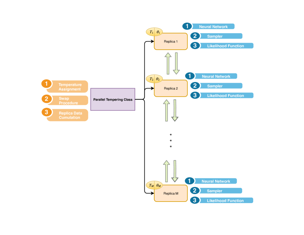
Figure 1: An overview of the different replica’s that are executed on a multi-processing architecture. Note that the main process controls the given replicas and enables them to exchange the neighboring replicas given the swap time and probability of exchange is satisfied.

The multi-core implementation takes into account operating system concepts such as interprocess communications when considering exchange of solutions between the neighboring replicas [31]. The implementation is done in multi-core fashion by which each replica runs on a single central processing unit (CPU). Figure 1 gives an overview of the different replicas that are executed on the multi-processing software wherein each replica runs on a separate core with inter-process communication for exchanging neighboring replicas. The main process runs on a separate core which controls the replicas and enables them to exchange the neighboring replicas given the swap interval and probability of exchange is satisfied. Each replica is allocated a fixed sampling time controlled by the number of iterations. The main process waits for all samplers to complete their required sampling till the swap interval iteration after which the samplers attempt configuration exchange. Once the replica reaches this junction, the main process proposes configuration swaps between adjacent samplers based on likelihoods of adjacent chains. Main process notifies the replicas post swapping to resume sampling with latest configurations in the chain for each replica. The process continues with the sampling and proposing swaps until the the maximum sampling time.

We utilize multi-processing software development packages for the resources to have efficient inter-process communication [31] taking into account the swapping of replicas at certain intervals in the iterations. We implement our own parallel tempering for multi-core architecture using the Python multiprocessing library [74] and release an open-source software package for the same given here . The software we developed is very generic and can be modified easily to suit a large set of applications.

4 Experiments and Results

This section presents the experimental evaluation of multi-core parallel tempering for Bayesian neural learning given selected time series prediction and classification problems.

4.1 Experimental Design

We present experimental design that features parallel tempering based on random-walk (PT-RW) and Langevin gradient (PT-LG) proposals based on [23]. We use geometric temperature spacing [75] to determine the temperature for each replica of the respective algorithms. In all experiments, we use a hybrid parallel tempering implementation where parallel tempering is used in the first stage that compromises of 60 percent of the sampling time. In the second stage, the framework changes to canonical MCMC where the temperature value of the replicas become 1. In this way, parallel tempering is used mostly for exploration or global search in the first phase which is followed by exploitation or local search in the second phase. Moreover, first 50 percent of samples are discarded as burn-in period required for convergence. This is a standard procedure in sampling methods used for Bayesian inference. Furthermore, the Langevin-gradient proposals are applied with a probability of 0.5 for every sample proposed. The effect of the learning rate used for the Langevin-gradient are evaluated in the experiments. The experiments are designed as follows.

• Evaluate effect of maximum temperature for a selected time series problem;

• Evaluate effect of swap interval for a selected time series problem;

• Evaluate effect of Langevin-gradient rate for a selected time series problem;

• Compare PT-RW and PT-LG for a range time series prediction problems;

• Compare PT-RW and PT-LG for pattern classification problems.

We used one hidden layer feedforward neural network where the number of hidden units was $h=5$ for time series prediction problems. In the case of pattern classification, the number of hidden layers is provided in Table 1. We evaluate the effect of the hyper-parameters in parallel tempering, which include the maximum geometric temperature spacing and swap interval for swapping neighboring replicas. Note that all experiments used 10 replicas with a multi-core implementation that was experimented using high-performance computing environment in order to ensure that each replica is executed on a separate core.

In random-walk proposals, we draw and add a Gaussian noise to the weights and biases of the network from a standard normal distribution, with mean of 0 and standard deviation of $0.025$. As given in Equation 4 whereas for $\eta$ (where $\eta$ is defined as $\eta=log(var(y-E(y|{\bf x}))$), the random-walk step is $0.2$. The random-walk step becomes the standard deviation when we draw the weights and $\eta$ from the normal distribution centered around $0$. The parameters of the priors (see Equation (6)) were set as ${\sigma}^{2}=25,{\nu}_{1}=0$ and ${\nu}_{2}=0$.

4.1.1 Time series problems

The benchmark problems used are Sunspot, Lazer, Mackey-Glass, Lorenz, Henon and Rossler time series. Takens’ embedding theorem [70] is applied with selected values as follows. Dimension, $D=4$ and time lag, $T=2$ is used for reconstruction of the respective time series into state-space vector as done in previous works [76, 77]. All the problems used first one thousand data points of the time series from which 60% was used for training and remaining for testing. The prediction performance is measured by root mean squared error as follows

$$RMSE=\sqrt{\frac{1}{N}\sum_{i=1}^{N}(y_{i}-\hat{y_{i}})^{2}}$$

where $y_{i}$ and $\hat{y_{i}}$ are the true value and the predicted value respectively. $N$ is the total length of the data. The maximum sampling time is set to 100,000 samples for the respective time series problems.

4.1.2 Pattern classification problems

We selected six pattern classification problems from University of California Irvine machine learning repository [78]. The problems were selected according to their size and complexity in terms of number of features and samples. We experiment with small datasets with small number of features (Iris and Cancer), then with small dataset with high number of features (Ionosphere). Moreover, three relatively large datasets with high number features, one with low number of classes (Bank-Market) and others with high number of classes (Pen-Digit and Chess) as shown in Table 1.

Table 1: Classification Dataset Description

Dataset	Instances	Attributes	Classes	Hidden Units
Iris	150	4	3	12
Breast Cancer	569	9	2	12
Ionosphere	351	34	2	50
Bank-Market	11162	20	2	50
Pen-Digit	10992	16	10	30
Chess	28056	6	18	25

4.2 Results: time series prediction

Table 2: Evaluate maximum geometric temperature

Max. temp.	Train (mean, best, std)	Test (mean, best, std)	Swap per.	Accept per.	Time (min.)
2	0.0639 0.0208 0.0292	0.0543 0.0184 0.0244	31.97	30.26	3.65
4	0.0599 0.0206 0.0299	0.0523 0.0176 0.0248	38.21	33.74	3.94
6	0.0656 0.0220 0.0299	0.0576 0.0210 0.0277	48.59	36.01	4.70
8	0.0692 0.0277 0.0311	0.0584 0.0209 0.0261	44.97	37.72	3.79
10	0.0635 0.0250 0.0293	0.0547 0.0212 0.0251	43.97	38.14	3.73

Table 3: Evaluate swap interval

Swap interval	Train (mean, best, std)	Test (mean, best, std)	Swap per.	Accept per.	Time (min.)
100	0.0628 0.0233 0.0286	0.0554 0.0213 0.0264	31.33	34.19	3.66
200	0.0608 0.0226 0.0308	0.0521 0.0194 0.0262	40.65	33.41	3.49
300	0.0657 0.0190 0.0328	0.0562 0.0173 0.0263	39.01	34.38	3.47
400	0.0648 0.0238 0.0281	0.0552 0.0214 0.0230	40.11	34.35	3.68
500	0.0676 0.0220 0.0310	0.0577 0.0190 0.0279	50.00	34.82	3.83
600	0.0621 0.0255 0.0266	0.0549 0.0209 0.0247	50.00	32.62	3.54
700	0.0614 0.0197 0.0320	0.0522 0.0169 0.0280	47.36	34.10	3.52
800	0.0739 0.0217 0.0291	0.0666 0.0214 0.0264	31.57	36.08	3.52

Table 4: Evaluate LG Rate

LG-frequency	Train (mean, best, std)	Test (mean, best, std)	Swap per.	Accept per.	Time (min.)
0	0.0628 0.0233 0.0286	0.0554 0.0213 0.0264	31.33	34.19	3.66
0.1	0.0539 0.0224 0.0286	0.0500 0.0238 0.0273	34.20	30.50	6.06
0.2	0.0361 0.0099 0.0261	0.0331 0.0083 0.0239	45.66	26.33	7.33
0.3	0.0346 0.0096 0.0226	0.0318 0.0077 0.0233	39.42	23.84	9.10
0.4	0.0365 0.0113 0.0249	0.0340 0.0107 0.0232	45.57	22.74	10.12
0.5	0.0451 0.0188 0.0266	0.0402 0.0177 0.0248	32.88	21.19	11.6
0.6	0.0464 0.0247 0.0245	0.0433 0.0205 0.0234	52.32	19.65	13.22
0.7	0.0396 0.0232 0.0234	0.0373 0.0214 0.0202	48.65	18.74	15.23
0.8	0.0350 0.0195 0.0230	0.0346 0.0168 0.0231	45.13	16.66	17.63

We first show results for effect of different parameter values for selected time series problem. Table 2 shows the performance of the PT-RW method for Lazer problem given different values of the maximum temperature of the geometric temperature ladder given fixed swap interval of 100 samples. We note that the maximum temperature has a direct effect on the swap probability. Higher values would implies that some of the replicas with high values of the temperature gives more opportunities for exploration as it allows the replica to get out of the local minimum while the replicas with lower temperature values focus on exploitation of a local region in the likelihood landscape. The results show that temperature value of 4 gives the best results in prediction denoted by lowest RMSE for training and test performance considering both the train and test datasets. It seems that the problems requires less lower swap rate as it needs to concentrate more on exploiting local region. Moving on, Table 3 shows the results for the changes in the swap interval that determines how often to calculate the swap probability for swapping given maximum geometric temperature of 4. Note that during swapping, the master process freezes all the replica sampling process and calculates the swap probability in order to swap between neighboring replicas. We note that there is not a major difference in the performance given the range of swap interval considered. Howsoever, the results show that the swap interval of 200 is best for time series problems. Furthermore, Table 4 shows the effects of the Langevin-gradient frequency (LG-frequency) where swap interval of 100 samples was used with learning rate of 0.1. We notice that the higher rate of using gradients review more time. This is due to the computational cost of calculating gradients for the given proposals. The LG-frequency of [0.2 - 0.4] shows the best results in prediction with moderate computational load. These values may be slightly different for the different problems.

Considering the hyper-parameters (maximum temperature, swap interval and LG-frequency) from previous results, Table 5 provides results for PT-RW and PT-LG for the selected problems. Note that we provide experimentation of two experimental setting for PT-LG (learning rate) where learning rate of 0.1 and 0.01 are used. The results show that PT-LG (0.1) gives the best performance in terms of training and test performance (RMSE) for Lazer, Sunspot, Lorenz and Henon problems. In other problems (Mackey, Rossler), it achieves similar performance when compared to PT-RW and PT-LG (0.01). We note that a highly significant improvement in results is made for the Henon and Lazer problems with PT-LG (0.1). We can infer that the learning rate is an important parameter to harness the advantage of Langevin-gradients. In terms of computational time, we notice that PT-LG is far more time consuming than PT-RW, due to the cost of calculating the gradients.

In terms of percentage of accepted proposals over the entire sampling process, PT-LG (0.1) has least acceptance percentage of the proposals. On the other hand, we notice that PT-RW has the highest acceptance percentage followed by PT-LG (0.01) . Moreover, the swap percentage is generally higher for PT-LG (0.1) when compared to others for most of the problems. It could be argued that the higher rate of accepted proposals deteriorates the results. This could imply that weaker proposals are accepted more often in these settings, hence there is emphasis on exploration rather than exploitation. The higher swap percentage indicates exploration over local minimums. Furthermore, small learning rate (0.01) forces the gradient to have little influence on the proposals and hence PT-LG (0.01) behaves more like PT-RW.

Table 5: Prediction Results

Dataset	Method	Train (mean, best, std)	Test (mean, best, std)	Swap per.	Accept per.	Time (min.)
Lazer	PT-RW	0.0640 0.0218 0.0325	0.0565 0.0209 0.0270	42.26	35.31	4.53
	PT-LG (0.10)	0.0383 0.0187 0.0240	0.0353 0.0161 0.0212	48.45	19.91	11.53
	PT-LG (0.01)	0.0446 0.0160 0.0283	0.0414 0.0160 0.0253	51.45	30.97	11.50
Sunspot	PT-RW	0.0242 0.0041 0.0170	0.0239 0.0050 0.0161	44.45	18.30	4.82
	PT-LG(0.10)	0.0199 0.0031 0.0155	0.0192 0.0033 0.0146	48.45	12.57	11.61
	PT-LG (0.01)	0.0215 0.0032 0.0168	0.0204 0.0034 0.0154	46.94	15.16	11.47
Mackey	PT-RW	0.0060 0.0005 0.0051	0.0061 0.0005 0.0051	42.11	8.19	4.59
	PT-LG (0.1)	0.0061 0.0009 0.0047	0.0062 0.0009 0.0048	49.10	5.72	11.68
	PT-LG (0.01)	0.0064 0.0008 0.0052	0.0065 0.0008 0.0053	48.58	8.38	11.43
Lorenz	PT-RW	0.0192 0.0033 0.0113	0.0171 0.0037 0.0094	39.48	14.48	4.45
	PT-LG (0.1)	0.0181 0.0018 0.0117	0.0157 0.0018 0.0094	50.37	9.66	11.48
	PT-LG (0.01)	0.0173 0.0023 0.0123	0.0147 0.0024 0.0095	46.30	11.91	11.42
Rossler	PT-RW	0.0173 0.0011 0.0144	0.0175 0.0011 0.0148	48.11	12.53	4.22
	PT-LG (0.1)	0.0172 0.0008 0.0154	0.0175 0.0009 0.0155	39.57	8.58	11.60
	PT-LG (0.01)	0.0171 0.0011 0.0136	0.0173 0.0011 0.0135	50.18	10.98	11.36
Henon	PT-RW	0.1230 0.0296 0.0167	0.1198 0.0299 0.0161	48.58	38.08	4.21
	PT-LG (0.1)	0.0201 0.0025 0.0146	0.0190 0.0029 0.0131	47.43	11.39	11.41
	PT-LG (0.01)	0.0992 0.0347 0.0221	0.0963 0.0341 0.0209	36.04	36.27	11.49

4.3 Results: classification

The multinomial likelihood given in Equation 8 is used for pattern classification experiments that compare PT-RW and PT-LG. We used maximum sampling time of 50,000 samples with LG-frequency of 0.5, swap interval of 100 and maximum temperature of 10. The results for the classification performance along with the time taken and acceptance for the respective dataset is provided in Table 6. We use PT-LG(learning rate) of 0.01 and 0.1 and compare the performance with random-walk (PT-RW) proposals. The results show that PT-LG(0.01) overall achieves the best training and generalization performance for all the given problems. PT-LG(0.1) has similar training and test performance when compared to PT-RW for certain problems (Bank and Pen-Digit) only. In majority of the cases PT-LG(0.1) outperforms PT-RW. We notice that the smaller datasets (Iris, Ionosphere and Cancer) have much higher acceptance percentage of proposals when compared to larger datasets. Furthermore, the higher computational cost of applying Langevin-gradients is evident in all the problems.

Table 6: Classification Results

Dataset	Method	Train (mean, best, std)	Test (mean, best, std)	Swap perc.	Accept perc.	Time (min.)
Iris	PT-RW	51.39 15.02 91.43	50.18 41.78 100.00	52.56	95.32	1.26
	PT-LG ( 0.1)	64.93 21.51 100.00	59.33 39.84 100.00	51.08	51.48	1.81
	PT-LG (0.01)	97.32 0.92 99.05	96.76 0.96 99.10	51.77	97.55	2.09
Ionosphere	PT-RW	68.92 16.53 91.84	51.29 30.73 91.74	50.61	89.32	3.50
	PT-LG (0.1)	65.78 10.87 85.71	84.63 9.54 96.33	47.83	45.46	4.70
	PT-LG (0.01)	98.55 0.55 99.59	92.19 2.92 98.17	51.77	92.40	5.07
Cancer	PT-RW	83.78 20.79 97.14	83.55 27.85 99.52	40.18	89.71	2.78
	PT-LG (0.1)	83.87 17.33 97.55	90.59 16.67 99.52	41.71	43.87	5.13
	PT-LG(0.01)	97.00 0.29 97.75	98.77 0.32 99.52	49.25	94.67	5.09
Bank	PT-RW	78.39 1.34 80.11	77.49 0.90 79.45	49.13	61.59	27.71
	PT-LG(0.1)	77.90 1.92 79.71	77.74 1.27 79.57	46.17	29.61	69.89
	PT-LG(0.01)	80.75 1.45 85.41	79.96 0.81 82.61	50.00	31.50	86.94
Pen-Digit	PT-RW	76.67 17.44 95.24	71.93 16.59 90.62	45.60	50.72	57.13
	PT-LG(0.1)	73.91 17.36 91.98	70.09 16.08 85.68	46.89	24.95	87.06
	PT-LG(0.01)	84.98 7.42 96.02	81.24 6.82 91.25	51.08	25.09	86.62
Chess	PT-RW	89.48 17.46 100.00	90.06 15.93 100.00	48.09	69.09	252.56
	PT-LG(0.1)	100.00 0.00 100.00	100.00 0.00 100.00	49.88	92.61	327.45
	PT-LG(0.1)	100.00 0.00 100.00	100.00 0.00 100.00	50.12	88.87	323.10

Figure 2: Posterior distribution with sampling trace-plot of a selected weight in the input-hidden layer for Iris problem given by PT-LG.

5 Discussion

We presented a multi-core implementation of parallel tempering with variations such as random-walk and Langevin-gradients for time series prediction and pattern classification problems. The goal is to harness the advantage of parallel computing for large datasets where thousands of samples are required for convergence for a posterior distribution. We demonstrated the concept using smaller time series prediction datasets in order to effectively study the effects of certain hyper-parameters. The experiments revealed that it is important to have the right hyper-parameter setting such as swap-interval and maximum temperature for geometric temperature spacing. Moreover, the learning rate used for Langevin-gradients can also be an issue given the type of problem, which also depends on the nature of the time series; whether it is synthetic or real-world problem and how much of noise and inconsistencies are present. We noticed that the Langevin-gradients has more effect since it improved the results further for real-world time series (Lazer and Sunspot problems). In certain cases, higher level of noise and chaotic behavior is present in synthetic time series, such as the Henon time series. In this case, the Langevin-gradient significantly improved performance. One needs to take into account the computational costs of calculating the gradients as shown in the results. Earlier, we found that rate of [0.2 - 0.3] gives the best performance in terms of accuracy in prediction and also computation time for time series problems. Hence, it is worthwhile to use lower values of LG-frequency. Furthermore, our implementation and experiments were limited to ten replicas, which could be increased for bigger datasets and problems.

In the case of classification problems, we observe that both variations of Langevin-gradient parallel tempering significantly improved the classification performance for majority of the problems. In some cases, the classification performance was slightly improved, however, Langevin-gradients have used high computational time in general. In general, we noticed that lower learning rate (0.01) had best performance for classification problem, but had little effect for the time series prediction problems. Therefore, the sampling is highly sensitive to the Langevin-gradient learning rate which needs to be tailored for the type of the problem. Furthermore, note that the rate at which the Langevin-gradient is applied adds to the computational cost. We need to further highlight that the parallel tempering is used mostly for exploration in the first phase of sampling and most of these values are discarded given 50 percent of burnin period. The second phase follows canonical MCMC sampling, while taking advantage of swap and also multi-core implementation for lowering computational time.

We tested small scale to medium scale classification problems that considered a few hundred to thousands of weights in the neural networks. Large number of neural network weights implies large scale inference which has been a challenge of Bayesian neural networks that have mainly been limited to small scale problems. Multi-core parallel tempering has demonstrated to have potential to be applied to deep learning that involve recurrent neural networks and convolution networks that typical deal with thousands to millions of weights. Although, millions of weights is a huge task for vision related problems, given the incorporation of Langevin-gradients, this could be possible. Another possibility is to use stochastic gradient descent implementation for Langevin-gradients with parallel tempering. We only considered calculation of gradient for entire datasets which could be difficult for big data problems. The deep learning literature has been constantly trying to improve learning methods that have novel methodologies to feature gradient information which can be used to give better proposals for inference via parallel tempering. This further opens up Bayesian inference for new neural network architectures such as long short-term memory recurrent networks (LSTMs) and generative adversarial networks [79, 80]. Furthermore, the use of efficient priors via transfer learning methods could also be a direction, where the priors feature knowledge learn from similar problems. Although uncertainty quantification is not a major requirement in some of the computer vision problems, in specific domains such as medical imaging and security, it is important to feature a Bayesian perspective that can be used to fuse many aspects of the data. For instance, three-dimensional (3D) face recognition could provide data from different sensors and cameras that can be fused given a Bayesian methodology. Furthermore, the framework proposed could be used for other models, such as in Earth science, which have expensive models that require efficient optimization or parameter estimation techniques [81]. Related work has explored the use of such framework for estimation of Solid Earth evolution models. In such problems, due to the complexity of the models, there is no scope for incorporating gradients since they are unavailable. In such cases, the need to develop heuristic methods for acquiring gradients is important. Hence, meta-heuristic and evolutionary algorithms could be incorporated with parallel tempering in models that do not have gradients. This could also apply to dynamic and complex neural network architectures, which has in past been addressed through neuro-evolution [82, 77].

6 Conclusions and Future Work

The major contributions of the paper can be highlighted as follows. 1.) the application of multi-core parallel tempering for enhancing Bayesian neural networks; 2.) the use of Langevin-gradient based proposals to enhance proposals in parallel tempering; 3.) and the application of the methodology to prediction and classification problems of varying degrees of complexity with performance evaluation in terms of the quality of decision making. The experimental analysis have shown that Langevin-gradient parallel tempering significantly improves the convergence with better prediction and classification performance. Moreover, additional computational costs are needed for Langevin-gradients and in future work such challenges can be tacked with more efficient gradient proposals. This motivates the use of the methodology for large scale problems that faced challenges with canonical implementations of Bayesian neural networks.

In future work, the implementation of parallel tempering in multi-core architectures can be applied to deep neutral network architectures and various applications that require uncertainty quantification in prediction or decision making process.

References

- Rumelhart et al. [????] D. E. Rumelhart, G. E. Hinton, R. J. Williams, Learning representations by back-propagating errors, Cognitive modeling 5 (????) 1.
- Zeiler [2012] M. D. Zeiler, Adadelta: an adaptive learning rate method, arXiv preprint arXiv:1212.5701 (2012).
- Cawley and Talbot [2007] G. C. Cawley, N. L. Talbot, Preventing over-fitting during model selection via bayesian regularisation of the hyper-parameters, Journal of Machine Learning Research 8 (2007) 841–861.
- Bengio [2000] Y. Bengio, Gradient-based optimization of hyperparameters, Neural computation 12 (2000) 1889–1900.
- Lawrence et al. [1996] S. Lawrence, C. L. Giles, A. C. Tsoi, What size neural network gives optimal generalization? Convergence properties of backpropagation, Technical Report, Institute for Advanced Computer Studies, University of Maryland, College Park, MD 20742, 1996.
- White and Ligomenides [1993] D. White, P. Ligomenides, Gannet: A genetic algorithm for optimizing topology and weights in neural network design, in: International Workshop on Artificial Neural Networks, Springer, pp. 322–327.
- Schmidhuber [2015] J. Schmidhuber, Deep learning in neural networks: An overview, Neural networks 61 (2015) 85–117.
- MacKay [1992] D. J. MacKay, A practical bayesian framework for backpropagation networks, Neural computation 4 (1992) 448–472.
- MacKay [1996] D. J. MacKay, Hyperparameters: Optimize, or integrate out?, in: Maximum entropy and Bayesian methods, Springer, 1996, pp. 43–59.
- MacKay [1995] D. J. MacKay, Probable networks and plausible predictions—a review of practical bayesian methods for supervised neural networks, Network: Computation in Neural Systems 6 (1995) 469–505.
- Robert [2014] C. Robert, Machine learning, a probabilistic perspective, 2014.
- Hastings [1970] W. K. Hastings, Monte carlo sampling methods using markov chains and their applications, Biometrika 57 (1970) 97–109.
- Metropolis et al. [1953] N. Metropolis, A. W. Rosenbluth, M. N. Rosenbluth, A. H. Teller, E. Teller, Equation of state calculations by fast computing machines, The journal of chemical physics 21 (1953) 1087–1092.
- Raftery and Lewis [1996] A. E. Raftery, S. M. Lewis, Implementing mcmc, Markov chain Monte Carlo in practice (1996) 115–130.
- van Ravenzwaaij et al. [2016] D. van Ravenzwaaij, P. Cassey, S. D. Brown, A simple introduction to markov chain monte–carlo sampling, Psychonomic bulletin & review (2016) 1–12.
- Banerjee et al. [2014] S. Banerjee, B. P. Carlin, A. E. Gelfand, Hierarchical modeling and analysis for spatial data, Crc Press, 2014.
- Neal [2012] R. M. Neal, Bayesian learning for neural networks, volume 118, Springer Science & Business Media, 2012.
- Jylänki et al. [2014] P. Jylänki, A. Nummenmaa, A. Vehtari, Expectation propagation for neural networks with sparsity-promoting priors., Journal of Machine Learning Research 15 (2014) 1849–1901.
- Hinton and Van Camp [1993] G. E. Hinton, D. Van Camp, Keeping the neural networks simple by minimizing the description length of the weights, in: Proceedings of the sixth annual conference on Computational learning theory, ACM, pp. 5–13.
- Li et al. [2016] C. Li, C. Chen, D. Carlson, L. Carin, Preconditioned stochastic gradient langevin dynamics for deep neural networks, in: Thirtieth AAAI Conference on Artificial Intelligence.
- Liang [2007] F. Liang, Annealing stochastic approximation monte carlo algorithm for neural network training, Machine Learning 68 (2007) 201–233.
- Kocadağlı and Aşıkgil [2014] O. Kocadağlı, B. Aşıkgil, Nonlinear time series forecasting with bayesian neural networks, Expert Systems with Applications 41 (2014) 6596–6610.
- Chandra et al. [2017] R. Chandra, L. Azizi, S. Cripps, Bayesian neural learning via langevin dynamics for chaotic time series prediction, in: D. Liu, S. Xie, Y. Li, D. Zhao, E.-S. M. El-Alfy (Eds.), Neural Information Processing.
- Srivastava et al. [2014] N. Srivastava, G. Hinton, A. Krizhevsky, I. Sutskever, R. Salakhutdinov, Dropout: A simple way to prevent neural networks from overfitting, The Journal of Machine Learning Research 15 (2014) 1929–1958.
- Gal and Ghahramani [2016] Y. Gal, Z. Ghahramani, Dropout as a bayesian approximation: Representing model uncertainty in deep learning, in: international conference on machine learning, pp. 1050–1059.
- Kendall and Gal [2017] A. Kendall, Y. Gal, What uncertainties do we need in bayesian deep learning for computer vision?, in: Advances in Neural Information Processing Systems, pp. 5580–5590.
- Marinari and Parisi [1992] E. Marinari, G. Parisi, Simulated tempering: a new monte carlo scheme, EPL (Europhysics Letters) 19 (1992) 451.
- Geyer and Thompson [1995] C. J. Geyer, E. A. Thompson, Annealing markov chain monte carlo with applications to ancestral inference, Journal of the American Statistical Association 90 (1995) 909–920.
- Patriksson and van der Spoel [2008] A. Patriksson, D. van der Spoel, A temperature predictor for parallel tempering simulations, Physical Chemistry Chemical Physics 10 (2008) 2073–2077.
- Hukushima and Nemoto [1996] K. Hukushima, K. Nemoto, Exchange monte carlo method and application to spin glass simulations, Journal of the Physical Society of Japan 65 (1996) 1604–1608.
- Lamport [1986] L. Lamport, On interprocess communication, Distributed computing 1 (1986) 86–101.
- Salakhutdinov et al. [2007] R. Salakhutdinov, A. Mnih, G. Hinton, Restricted boltzmann machines for collaborative filtering, in: Proceedings of the 24th international conference on Machine learning, ACM, pp. 791–798.
- Hinton et al. [2006] G. E. Hinton, S. Osindero, Y.-W. Teh, A fast learning algorithm for deep belief nets, Neural computation 18 (2006) 1527–1554.
- Desjardins et al. [2010] G. Desjardins, A. Courville, Y. Bengio, P. Vincent, O. Delalleau, Tempered markov chain monte carlo for training of restricted boltzmann machines, in: Proceedings of the thirteenth international conference on artificial intelligence and statistics, pp. 145–152.
- Brakel et al. [2012] P. Brakel, S. Dieleman, B. Schrauwen, Training restricted boltzmann machines with multi-tempering: harnessing parallelization, in: International Conference on Artificial Neural Networks, Springer, pp. 92–99.
- Fischer and Igel [2015] A. Fischer, C. Igel, A bound for the convergence rate of parallel tempering for sampling restricted boltzmann machines, Theoretical Computer Science 598 (2015) 102 – 117.
- Pascanu et al. [2013] R. Pascanu, T. Mikolov, Y. Bengio, On the difficulty of training recurrent neural networks, in: International Conference on Machine Learning, pp. 1310–1318.
- Swendsen and Wang [1986] R. H. Swendsen, J.-S. Wang, Replica monte carlo simulation of spin-glasses, Physical review letters 57 (1986) 2607.
- Hansmann [1997] U. H. Hansmann, Parallel tempering algorithm for conformational studies of biological molecules, Chemical Physics Letters 281 (1997) 140–150.
- Sen and Stoffa [1996] M. K. Sen, P. L. Stoffa, Bayesian inference, gibbs’ sampler and uncertainty estimation in geophysical inversion, Geophysical Prospecting 44 (1996) 313–350.
- Maraschini and Foti [2010] M. Maraschini, S. Foti, A monte carlo multimodal inversion of surface waves, Geophysical Journal International 182 (2010) 1557–1566.
- Rathore et al. [2005] N. Rathore, M. Chopra, J. J. de Pablo, Optimal allocation of replicas in parallel tempering simulations, The Journal of chemical physics 122 (2005) 024111.
- Katzgraber et al. [2006] H. G. Katzgraber, S. Trebst, D. A. Huse, M. Troyer, Feedback-optimized parallel tempering monte carlo, Journal of Statistical Mechanics: Theory and Experiment 2006 (2006) P03018.
- Bittner et al. [2008] E. Bittner, A. Nußbaumer, W. Janke, Make life simple: Unleash the full power of the parallel tempering algorithm, Physical review letters 101 (2008) 130603.
- Calvo [2005] F. Calvo, All-exchanges parallel tempering, The Journal of chemical physics 123 (2005) 124106.
- Fielding et al. [2011] M. Fielding, D. J. Nott, S.-Y. Liong, Efficient mcmc schemes for computationally expensive posterior distributions, Technometrics 53 (2011) 16–28.
- Liu et al. [2005] P. Liu, B. Kim, R. A. Friesner, B. J. Berne, Replica exchange with solute tempering: A method for sampling biological systems in explicit water, Proceedings of the National Academy of Sciences 102 (2005) 13749–13754.
- Li et al. [2009] Y. Li, M. Mascagni, A. Gorin, A decentralized parallel implementation for parallel tempering algorithm, Parallel Computing 35 (2009) 269 – 283.
- Karimi et al. [2011] K. Karimi, N. Dickson, F. Hamze, High-performance physics simulations using multi-core cpus and gpgpus in a volunteer computing context, The International Journal of High Performance Computing Applications 25 (2011) 61–69.
- Mingas et al. [2017] G. Mingas, L. Bottolo, C.-S. Bouganis, Particle mcmc algorithms and architectures for accelerating inference in state-space models, International Journal of Approximate Reasoning 83 (2017) 413–433.
- Musiani and Giorgetti [2017] F. Musiani, A. Giorgetti, Protein aggregation and molecular crowding: Perspectives from multiscale simulations, in: International review of cell and molecular biology, volume 329, Elsevier, 2017, pp. 49–77.
- Xie et al. [2010] Y. Xie, J. Zhou, S. Jiang, Parallel tempering monte carlo simulations of lysozyme orientation on charged surfaces, The Journal of chemical physics 132 (2010) 02B602.
- Tharrington and Jordan [2003] A. N. Tharrington, K. D. Jordan, Parallel-tempering monte carlo study of (h2o) n= 6-9, The Journal of Physical Chemistry A 107 (2003) 7380–7389.
- Littenberg and Cornish [2009] T. B. Littenberg, N. J. Cornish, Bayesian approach to the detection problem in gravitational wave astronomy, Physical Review D 80 (2009) 063007.
- Reid et al. [2013] A. Reid, E. V. Bonilla, L. McCalman, T. Rawling, F. Ramos, Bayesian joint inversions for the exploration of Earth resources, in: IJCAI, pp. 2877–2884.
- Richard and Lippmann [1991] M. D. Richard, R. P. Lippmann, Neural network classifiers estimate bayesian a posteriori probabilities, Neural computation 3 (1991) 461–483.
- Krogh and Hertz [1992] A. Krogh, J. A. Hertz, A simple weight decay can improve generalization, in: Advances in neural information processing systems, pp. 950–957.
- Auld et al. [2007] T. Auld, A. W. Moore, S. F. Gull, Bayesian neural networks for Internet traffic classification, IEEE Transactions on neural networks 18 (2007) 223–239.
- Neal et al. [2011] R. M. Neal, et al., Mcmc using hamiltonian dynamics, Handbook of Markov Chain Monte Carlo 2 (2011).
- Welling and Teh [2011] M. Welling, Y. W. Teh, Bayesian learning via stochastic gradient langevin dynamics, in: Proceedings of the 28th International Conference on Machine Learning (ICML-11), pp. 681–688.
- Chen et al. [2016] C. Chen, D. Carlson, Z. Gan, C. Li, L. Carin, Bridging the gap between stochastic gradient mcmc and stochastic optimization, in: Artificial Intelligence and Statistics, pp. 1051–1060.
- Liang [2005] F. Liang, Bayesian neural networks for nonlinear time series forecasting, Statistics and computing 15 (2005) 13–29.
- Hippert and Taylor [2010] H. S. Hippert, J. W. Taylor, An evaluation of bayesian techniques for controlling model complexity and selecting inputs in a neural network for short-term load forecasting, Neural networks 23 (2010) 386–395.
- Mirikitani and Nikolaev [2010] D. T. Mirikitani, N. Nikolaev, Recursive bayesian recurrent neural networks for time-series modeling, IEEE Transactions on Neural Networks 21 (2010) 262–274.
- Wan [1990] E. A. Wan, Neural network classification: A bayesian interpretation, IEEE Transactions on Neural Networks 1 (1990) 303–305.
- Cho et al. [2011] K. Cho, A. Ilin, T. Raiko, Improved learning of gaussian-bernoulli restricted boltzmann machines, in: International conference on artificial neural networks, Springer, pp. 10–17.
- Cho et al. [2010] K. Cho, T. Raiko, A. Ilin, Parallel tempering is efficient for learning restricted boltzmann machines, in: Neural Networks (IJCNN), The 2010 International Joint Conference on, IEEE, pp. 1–8.
- Desjardins et al. [2010] G. Desjardins, A. Courville, Y. Bengio, Adaptive parallel tempering for stochastic maximum likelihood learning of rbms, arXiv preprint arXiv:1012.3476 (2010).
- Desjardins et al. [2014] G. Desjardins, H. Luo, A. Courville, Y. Bengio, Deep tempering, arXiv preprint arXiv:1410.0123 (2014).
- Takens [1981] F. Takens, Detecting strange attractors in turbulence, in: Dynamical Systems and Turbulence, Warwick 1980, Lecture Notes in Mathematics, 1981, pp. 366–381.
- Earl and Deem [2005] D. J. Earl, M. W. Deem, Parallel tempering: Theory, applications, and new perspectives, Physical Chemistry Chemical Physics 7 (2005) 3910–3916.
- Neal [1996] R. M. Neal, Sampling from multimodal distributions using tempered transitions, Statistics and computing 6 (1996) 353–366.
- Chandra et al. [2017] R. Chandra, L. Azizi, S. Cripps, Bayesian neural learning via langevin dynamics for chaotic time series prediction, in: Neural Information Processing - 24th International Conference, ICONIP 2017, Guangzhou, China, November 14-18, 2017, Proceedings, Part V, pp. 564–573.
- Singh et al. [2013] N. Singh, L.-M. Browne, R. Butler, Parallel astronomical data processing with python: Recipes for multicore machines, Astronomy and Computing 2 (2013) 1–10.
- Kone and Kofke [2005] A. Kone, D. A. Kofke, Selection of temperature intervals for parallel-tempering simulations, The Journal of chemical physics 122 (2005) 206101.
- Chandra et al. [2018] R. Chandra, Y.-S. Ong, C.-K. Goh, Co-evolutionary multi-task learning for dynamic time series prediction, Applied Soft Computing 70 (2018) 576 – 589.
- Chandra et al. [2017] R. Chandra, Y.-S. Ong, C.-K. Goh, Co-evolutionary multi-task learning with predictive recurrence for multi-step chaotic time series prediction, Neurocomputing 243 (2017) 21–34.
- Asuncion and Newman [2007] A. Asuncion, D. Newman, UCI machine learning repository, 2007.
- Hochreiter and Schmidhuber [1997] S. Hochreiter, J. Schmidhuber, Long short-term memory, Neural computation 9 (1997) 1735–1780.
- Goodfellow et al. [2014] I. Goodfellow, J. Pouget-Abadie, M. Mirza, B. Xu, D. Warde-Farley, S. Ozair, A. Courville, Y. Bengio, Generative adversarial nets, in: Advances in neural information processing systems, pp. 2672–2680.
- Chandra et al. [2018] R. Chandra, R. D. Müller, R. Deo, N. Butterworth, T. Salles, S. Cripps, Multi-core parallel tempering bayeslands for basin and landscape evolution, CoRR abs/1806.10939 (2018).
- Potter and De Jong [2000] M. A. Potter, K. A. De Jong, Cooperative coevolution: An architecture for evolving coadapted subcomponents, Evol. Comput. 8 (2000) 1–29.