Bautin bifurcation in delayed reaction-diffusion systems with application to the Segel-Jackson model

Abstract

In this paper, we present an algorithm for deriving the normal forms of Bautin bifurcations in reaction-diffusion systems with time delays and Neumann boundary conditions. On the center manifold near a Bautin bifurcation, the first and second Lyapunov coefficients are calculated explicitly, which completely determine the dynamical behavior near the bifurcation point. As an example, the Segel-Jackson predator-prey model is studied. Near the Bautin bifurcation we find the existence of fold bifurcation of periodic orbits, as well as subcritical and supercritical Hopf bifurcations. Both theoretical and numerical results indicate that solutions with small (large) initial conditions converge to stable periodic orbits (diverge to infinity).

1 Introduction

In recent years, Hopf bifurcation in reaction-diffusion systems with time delays has been widely studied Faria2001 ; Su-Wei-Shi . The results are used to interpret the oscillation behaviors in many subjects, such as, biology Chen ; Yi , chemistry Wei , and epidemics Jin , etc. The authors usually investigated the change of stability of equilibria and the existence of Hopf bifurcations. Furthermore, they calculated the normal forms near the Hopf bifurcations to determine the stability of bifurcating periodic solutions and direction of Hopf bifurcations. The framework of deriving normal forms is due to the center manifold reduction technique introduced in Yi ; Hassard ; Wu ; Lin .

As is known to all, supercritical Hopf bifurcations with negative first Lyapunov coefficient lead a system to stable periodic orbits at the side of bifurcation point that the equilibrium becomes unstable; whereas subcritical Hopf bifurcations with positive first Lyapunov coefficient induce unstable periodic orbits at the side of bifurcation point that the equilibrium becomes stable. General theory about Hopf bifurcation can be found in Holmes ; Wiggins2 ; Kuz for ordinary differential equations, in Hassard for functional differential equations, and in Wu ; Henry for partial differential equations or partial functional differential equations. If we introduce another parameter and with the change of that parameter, Hopf bifurcation points forms a curve in the two-parameter plane. Thus, at the intersection of the supercritical Hopf bifurcation and subcritical Hopf bifurcation curves, there will be a point with zero first Lyapunov coefficient that makes possible Bautin bifurcation happen which is of codimension two Holmes ; Wiggins2 ; Kuz ; jmaa . Near a Bautin bifurcation, the dynamical behavior of a system is quite complicated: the bifurcation point separates branches of subcritical and supercritical Hopf bifurcations in the parameter space. For parameter values near the singularity, the system has two limit cycles which collide and disappear via a fold bifurcation of periodic orbits.

So far, there are few papers on codimension two bifurcations in delay equation, most of which focus in retarded functional differential equationsGuo ; Jiang , and neutral functional differential equations Niu1 ; Niu2 . The study on codimension two bifurcations of delayed reaction-diffusion equations just begins in recent few years, and most of which are about Turing-Hopf bifurcation Song , Hopf-zero bifurcationAn or Double Hopf bifurcationDu . Near these bifurcations the spatially non-homogeneous steady-state solutions have been found as well as periodic solutions and quasi-periodic solutions. Bautin bifurcations have been found and analyzed in ordinary differential equations ode1 ; ode2 ; ode3 ; ode4 or in delay differential equations Xu1 ; Xu2 ; Ion . However, to our best knowledge, there are not any research papers found in literature about Bautin bifurcations in reaction-diffusion systems with time delays.

Motivated by such a consideration, in this paper we will give universal derivations of the first and second Lyapunov coefficients for Bautin bifurcations in reaction-diffusion equations with time delays, then the normal form of Bautin bifurcations is given and has two different kinds of bifurcation diagrams. The results are then applied to a Segel-Jackson prey-predator modelWang ; Segel

$$\left\{\begin{array}[]{l}\frac{\partial u(x,t)}{\partial t}=d\Delta u(x,t)+[1+ku(x,t)]u(x,t)-au(x,t)v(x,t)\\ \frac{\partial v(x,t)}{\partial t}=\Delta v(x,t)+u(x,t-\tau)v(x,t-\tau)-v^{2}(x,t)\end{array}~{}~{}~{}~{}~{}x\in[0,l\pi],t>0.\right.$$ (1)

In such a system with time delay and homogeneous boundary conditions, we find that Bautin bifurcation appears in $(k,\tau)$ plane. Both subcritical and supercritical Hopf bifurcations are found theoretically near the bifurcation point.

The rest part of the paper will be organized as follows. In section 2, the fifth-order normal form near a pair of imaginary roots in a general reaction-diffusion system of $N$ equations with time delays are derived, from which detailed and explicit formulae to determine the first and second Lyapunov coefficients for Bautin bifurcation are given. In section 3, we apply the results to a Segel-Jackson model, in which we find a Bautin bifurcation, and both subcritical and supercritical Hopf bifurcations are theoretically analyzed. To support the results some simulations are performed to illustrate the dynamical behaviors near the Bautin bifurcation. Finally a conclusion section completes this paper.

2 Bautin bifurcation in a reaction-diffusion system with time delays

We consider the following general form of a reaction-diffusion system with delays,

$$\frac{dU(t)}{dt}=D(\mu)\Delta U(t)+L(\mu)(U_{t})+F(\mu,U_{t}).$$ (2)

Here the state variable $U$ maps $[-1,+\infty)$ to $X$, and the state space is

$$X=\left\{(u_{1},u_{2},\ldots,u_{N})\in\left[{H^{2}(0,l\pi)}\right]^{N}:\left.\left(\frac{du_{1}}{dx},\frac{du_{2}}{dx},\ldots,\frac{du_{N}}{dx}\right)\right|_{x=0,l\pi}=0\right\}.$$

Notice that here we use homogeneous Neumann boundary conditions, and a one dimensional space interval $[0,l\pi]$. Using the general notation of delayed equations Wu , the state $U_{t}$ in phase space $\mathscr{C}:=C([-1,0],X)$ is defined by $U_{t}(\theta)=U(t+\theta)$ for any $\theta\in[-1,0]$. The bifurcation parameter $\mu=(\mu_{1},\mu_{2})\in\mathbb{R}^{2}$. The diffusion matrix $D(\mu)=\mathrm{diag}~{}(d_{1}(\mu),d_{2}(\mu)),\ldots,d_{n}(\mu))$.  $L:{\mathbb{R}}^{2}\times\mathscr{C}\rightarrow X$ is a bounded linear operator. $F:{\mathbb{R}}^{2}\times\mathscr{C}\rightarrow X$ is a $C^{k}$ $(k\geq 5)$ function of the form $(F_{1},F_{2},\ldots,F_{N})^{\rm T}$ and satisfies $F(\mu,0)=0$ and $D_{\varphi}F(\mu,0)=0$, which means $U_{t}=0$ is a steady states of system (2).

The linearized equation of system (2) at $U_{t}=0$ is

$$\frac{dU(t)}{dt}=D(\mu)\Delta U(t)+L(\mu)U_{t}.$$ (3)

Since we are about to calculate the fifth order normal form at a Bautin bifurcation, we first assume that when $\mu\in V$, with $V$ representing some neighbourhood of the origin in $\mathbb{R}^{2}$, the characteristic equation of (3)

$$det\left[\lambda{\rm{I}}+\frac{n^{2}}{l^{2}}D(\mu)-L(\mu)(\rm e^{\lambda\cdot}I)\right]=0$$ (4)

has a pair of roots $\alpha(\mu)\pm\rm i\omega(\mu)$ for some $n=n_{0}$ where $\alpha(\mu)$ and $\omega(\mu)$ are both continuously differentiable, and $\alpha(0)=0$, $\omega(0)=\omega_{0}>0$. We further assume that all the other roots of (4) have negative real parts for $\mu\in V$. Thus the center manifold will be locally attractive and the local dynamical behaviors of (3) will be governed by the normal form on the center manifold Lin .

The solution operator of Eq.(2) generates a $C_{0}$-semigroup with the infinitesimal generator $A_{\mu}$ defined by

$$A_{\mu}\phi=\left\{\begin{array}[]{ll}\dot{\phi}(\theta),&\theta\in[-1,0),\\ D(\mu)\Delta\phi(0)+L(\mu)\phi,&\theta=0.\end{array}\right.$$ (5)

The domain of $A_{\mu}$ is chosen by

$${\rm dom}(A_{\mu}):=\{\phi\in\mathscr{C}:\dot{\phi}\in\mathscr{C},\phi(0)\in{\rm dom}(\Delta),\dot{\phi}(0)=D(\mu)\Delta\phi(0)+L(\mu)\phi\}.$$

We rewrite Eq.(2) as an abstract ordinary differential equation

$$\frac{d}{dt}{U_{t}}=A_{\mu}U_{t}+R(\mu,U_{t})$$ (6)

with the nonlinearity

$$R(\mu,U_{t})(\theta)=\left\{\begin{array}[]{ll}0,&\theta\in[-1,0),\\ F(\mu,U_{t}),&\theta=0.\end{array}\right.$$

Write the Fourier basis of $X$ by $\{b_{n}e_{1},b_{n}e_{2},\ldots,b_{n}e_{N}\}_{n=0}^{+\infty}$ with $e_{1}=(1,0,\ldots,0)^{\rm T}$, $e_{2}=(0,1,\ldots,0)^{\rm T},\ldots,$ $e_{N}=(0,0,\ldots,1)^{\rm T}$, and $b_{n}=\frac{\cos\frac{nx}{l}}{\|\cos\frac{nx}{l}\|_{L_{2}}}$. Here the $L_{2}$ norm is

$$\|\cos\frac{nx}{l}\|_{L_{2}}=\left\{\begin{array}[]{l}\sqrt{\frac{1}{l\pi}},~{}~{}n=0,\\ \sqrt{\frac{2}{l\pi}},~{}~{}n\neq 0.\end{array}\right.$$

Also denote by $\beta_{n}=(b_{n},b_{n},\ldots,b_{n})^{\rm T}$, then for any $\phi=(\phi^{(1)},\phi^{(2)},\ldots,\phi^{(N)})^{\rm T}\in\mathscr{C}$, we can define $\phi_{n}=<\phi,\beta_{n}>=(<\phi^{(1)},b_{n}>,<\phi^{(2)},b_{n}>,\ldots,<\phi^{(N)},b_{n}>)^{\rm T}$.

Now we have the action of $A_{\mu}$ on $\phi_{n}b_{n}$, denoted by $A_{\mu,n}$ as

$$A_{\mu,n}(\phi_{n}b_{n})=\left\{\begin{array}[]{l}\dot{\phi}(\theta)b_{n},\theta\in[-1,0),\\ \int_{-1}^{0}d\eta_{n}(\mu,\theta)\phi_{n}(\theta)b_{n},\theta=0,\end{array}\right.$$

with the function of bounded variation $\eta_{n}$ satisfying

$$-\frac{n^{2}}{l^{2}}D(\mu)\phi_{n}(0)+L_{\mu}(\phi_{n})=\int_{-1}^{0}d\eta_{n}(\mu,\theta)\phi_{n}(\theta).$$

Consider the adjoint operator of $A_{0}$, $A^{\ast}$ given by

$$A^{\ast}\varphi(s)=\left\{\begin{array}[]{ll}-\dot{\varphi}(s),&s\in(0,1],\\ \sum\limits_{n=0}^{\infty}\int_{-1}^{0}d\eta_{n}^{\textrm{T}}(0,t)\varphi_{n}(-t)b_{n},&s=0,\end{array}\right.$$

for some $\varphi\in\mathscr{C}^{\ast}=\mathscr{C}([0,1],X)$ and $\varphi_{n}=<\varphi,b_{n}>$. According to the formal adjoint theory given in Wu ; Hale , we define the bilinear form by

$$(\varphi,\phi)=\sum_{k,j=0}^{\infty}(\varphi_{k},\phi_{j})_{c}\int_{0}^{l\pi}b_{k}b_{j}dx.$$ (7)

In fact, $\int_{0}^{l\pi}b_{k}b_{j}dx=0$, $\forall k\neq j$. Thus, we only need to define $(\varphi_{n},\phi_{n})_{c}$ from Hassard ; Wu , as

$$(\varphi_{n},\phi_{n})_{c}=\bar{\varphi}_{n}^{\textrm{T}}(0)\phi_{n}(0)-\int_{-1}^{0}\int_{\xi=0}^{\theta}\bar{\varphi}_{n}^{\textrm{T}}(\xi-\theta)d\eta_{n}(0,\theta)\phi_{n}(\xi)d\xi.$$

Let $q(\theta)b_{n_{0}}$ and $q^{\ast}(s)b_{n_{0}}$ be the eigenfunctions of $A_{0}$ and $A^{\ast}$ corresponding to $\rm i\omega_{0}$ and $-\rm i\omega_{0}$ respectively, with $({q^{\ast}},q)_{c}=1,(q^{\ast},\bar{q})_{c}=0$.

Write the centerspace

$$P=\{zqb_{n_{0}}+\bar{z}\bar{q}b_{n_{0}}|z\in\mathbb{C}\}$$

and its orthogonal complement space

$$Q=\{\phi\in\mathscr{C}|(q^{\ast}b_{n_{0}},\phi)=0~{}and~{}(\bar{q}^{\ast}b_{n_{0}},\phi)=0\},$$

then $\mathscr{C}=P\bigoplus Q$ and the state variable $U_{t}$ of Eq.(6) could be decomposed by

$$U_{t}=z(t)q(\cdot)b_{n_{0}}+\bar{z}(t)\bar{q}(\cdot)b_{n_{0}}+W(t,\cdot)$$ (8)

where $W(t,\cdot)\in Q.$

Obviously $z(t)=(q^{\ast}b_{n_{0}},U_{t})$ and $W(t,\theta)=U_{t}(\theta)-2{\rm Re}\{z(t)q(\theta)b_{n_{0}}\}$. Thus, we have

$$\dot{z}(t)=\textrm{i}\omega_{0}z(t)+\bar{q}^{\ast\textrm{T}}(0)<F(0,U_{t}),\beta_{n_{0}}>,$$ (9)

where the nonlinear term is given by

$$<F,\beta_{n}>=(<F_{1},b_{n}>,<F_{2},b_{n}>,\ldots,<F_{N},b_{n}>)^{\textrm{T}}.$$

Using the center manifold theorem Wu ; Lin , $W(t,\cdot)$ can be expressed by a series of $z$ and $\bar{z}$, starting at quadratic terms

$$W(t,\cdot)=W(z,\bar{z},\cdot)=\sum\limits_{i+j\geq 2}W_{ij}(\cdot)\frac{z^{i}\bar{z}^{j}}{i!j!}$$ (10)

where $z$ and $\bar{z}$ are approximately the local coordinates for center manifold $\mathscr{C}_{0}$ in two directions $qb_{n_{0}}$ and $\bar{q}b_{n_{0}}$, respectively. For solution $U_{t}\in\mathscr{C}_{0},$ we have $U_{t}=z(t)q(\cdot)b_{n_{0}}+\bar{z}(t)\bar{q}(\cdot)+W(z(t),\bar{z}(t),\theta)$ and denote by

$$F(0,U_{t})|_{\mathscr{C}_{0}}=\tilde{F}(0,z,\bar{z}).$$

We write the Taylor formula

$$\tilde{F}(0,z,\bar{z})=\sum\limits_{i+j\geq 2}\frac{\partial^{(i+j)}\tilde{F}}{\partial^{i}z\partial^{j}\bar{z}}\frac{z^{i}\bar{z}^{j}}{i!j!}.$$

Now the equation (9) on the center manifold is expressed by

$$\dot{z}(t)=\textrm{i}\omega_{0}z(t)+g(z(t),\bar{z}(t)).$$ (11)

In order to calculate the normal form, we expand

$$g(z,\bar{z})=\sum\limits_{i+j\geq 2}g_{ij}\frac{z^{i}\bar{z}^{j}}{i!j!}.$$ (12)

According to the theory about normal form at a pair of imaginary roots Kuz . We have the normal form till fifth order given by

$$\dot{z}=(\nu(\mu)+i)z+l_{1}(\mu)z^{2}\bar{z}+l_{2}(\mu)z^{3}{\bar{z}}^{2}+O(|z|^{6})$$ (13)

with $\nu(\mu)=\frac{\alpha(\mu)}{\omega(\mu)}$,

$$l_{1}(\mu)=\frac{1}{2\omega_{0}}\left({\rm Re}g_{21}-\frac{1}{\omega_{0}}{{\rm Im}}\{g_{20}g_{11}\}\right)$$ (14)

and

$$\begin{array}[]{rl}&12l_{2}(\mu)=\frac{1}{\omega_{0}}{\rm Re}{g_{32}}\\ &~{}~{}+\frac{1}{\omega_{0}^{2}}{{\rm Im}}\left\{g_{20}\bar{g}_{31}-g_{11}(4g_{31}+3\bar{g}_{22})-\frac{1}{3}g_{02}(g_{40}+\bar{g}_{13})-g_{30}g_{12}\right\}\\ &~{}~{}+\frac{1}{\omega_{0}^{3}}{\rm Re}\left\{g_{20}\left[\bar{g}_{11}(3g_{12}-\bar{g}_{30})+g_{02}\left(\bar{g}_{12}-\frac{1}{3}g_{30}\right)+\frac{1}{3}\bar{g}_{02}g_{03}\right]\right\}\\ &~{}~{}+\frac{1}{\omega_{0}^{3}}{\rm Re}\left\{g_{11}\left[\bar{g}_{02}\left(\frac{5}{3}\bar{g}_{30}+3g_{12}\right)+\frac{1}{3}g_{02}\bar{g}_{03}-4g_{11}g_{30}\right]\right\}\\ &~{}~{}+\frac{3}{\omega_{0}^{3}}{{\rm Im}}\{g_{20}g_{11}\}{{\rm Im}}\{g_{21}\}+\frac{1}{\omega_{0}^{4}}{{\rm Im}}\{g_{11}\bar{g}_{02}[\bar{g}_{20}^{2}-3\bar{g}_{20}g_{11}-4g_{11}^{2}\}\\ &~{}~{}+\frac{1}{\omega_{0}^{4}}{{\rm Im}}\left\{g_{11}g_{20}\right\}[3{\rm Re}\{g_{11}g_{20}\}-2|g_{02}|^{2}].\end{array}$$ (15)

Notice that some $g_{ij}$’s may depend on the form of $W_{ij}$. By using (6) and (8), we have

$$\begin{array}[]{ll}\dot{W}&=\dot{U_{t}}-\dot{z}qb_{n_{0}}-\dot{\bar{z}}\bar{q}b_{n_{0}}\\ &=\left\{\begin{array}[]{ll}A_{0}W-2{\rm Re}\{g(z,\bar{z})q(\theta)\}b_{n_{0}},&\theta\in[-r,0)\\ A_{0}W-2{\rm Re}\{g(z,\bar{z})q(\theta)\}b_{n_{0}}+\tilde{F},&\theta=0\end{array}\right.\\ &:=A_{0}W+H(z,\bar{z},\theta).\end{array}$$ (16)

Again, expending $H(z,\bar{z},\theta)$ as

$$H(z,\bar{z})=\sum\limits_{i+j\geq 2}H_{ij}\frac{z^{i}\bar{z}^{j}}{i!j!},$$ (17)

we have

$$H_{ij}(\theta)=\left\{\begin{array}[]{ll}-g_{ij}q(\theta)b_{n_{0}}-\bar{g}_{ji}\bar{q}(0)b_{n_{0}},&\theta\in[-r,0)\\ -g_{ij}q(0)b_{n_{0}}-\bar{g}_{ji}\bar{q}(0)b_{n_{0}}+\frac{\partial^{(i+j)}\tilde{F}}{\partial^{i}z\partial^{j}\bar{z}},&\theta=0\end{array}\right.$$

and

$$\begin{array}[]{l}(A_{0}-2\rm i\omega_{0}I)W_{20}(\theta)=-H_{20}(\theta),~{}A_{0}W_{11}(\theta)=-H_{11}(\theta),\\ (A_{0}+2\rm i\omega_{0}I)W_{02}(\theta)=-H_{02}(\theta),\\ (A_{0}-3\rm i\omega_{0}I)W_{30}(\theta)-3g_{20}W_{20}(\theta)-3\bar{g}_{02}W_{11}(\theta)=-H_{30}(\theta),\\ (A_{0}-\rm i\omega_{0}I)W_{21}(\theta)-(g_{20}+2\bar{g}_{11})W_{11}(\theta)-2g_{11}W_{20}(\theta)-\bar{g}_{02}W_{02}(\theta)=-H_{21}(\theta),\\ (A_{0}+{\rm i}\omega_{0}I)W_{12}(\theta)-(\bar{g}_{20}+2g_{11})W_{11}(\theta)-2\bar{g}_{11}W_{02}(\theta)-g_{02}W_{20}(\theta)=-H_{12}(\theta),\\ (A_{0}+3{\rm i}\omega_{0}I)W_{03}(\theta)-3g_{02}W_{11}(\theta)-3\bar{g}_{20}W_{02}(\theta)=-H_{03}(\theta),\\ (A_{0}-2{\rm i}\omega_{0}I)W_{31}(\theta)-3(g_{20}+\bar{g}_{11})W_{21}(\theta)-(g_{30}+3\bar{g}_{12})W_{11}(\theta)-3g_{11}W_{30}(\theta)\\ ~{}~{}~{}~{}-3g_{21}W_{20}(\theta)-\bar{g}_{03}W_{02}(\theta)-3\bar{g}_{02}W_{12}(\theta)=-H_{31}(\theta),\\ A_{0}W_{22}(\theta)-g_{02}W_{30}(\theta)-(g_{20}+4\bar{g}_{11})W_{12}(\theta)-2(g_{21}+\bar{g}_{21})W_{11}(\theta)-2g_{12}W_{20}(\theta)\\ ~{}~{}~{}~{}-(\bar{g}_{20}+4g_{11})W_{21}(\theta)-2\bar{g}_{12}W_{02}(\theta)-\bar{g}_{02}W_{03}(\theta)=-H_{22}(\theta).\end{array}$$ (18)

Recalling the definition of $A_{0}$ in (5), we know (18) is actually a group of ordinary differential equations about $W_{ij}(\theta)$ with some given boundary conditions, solving which the explicit expressions of $W_{ij}$ and $g_{ij}$ are finally obtained.

According to the general results about Bautin bifurcations in Holmes , we assume $l_{1}(0)=0$, $l_{2}(0)\neq 0$ and the map $\mu\mapsto(\nu(\mu),l_{1}(\mu))$ is regular at $\mu=0$, then the system undergoes a Bautin bifurcation. Precisely, the bifurcation diagram is given by Figure 1.

Following the results given in Holmes , we know that near the Bautin bifurcation, when $l_{2}(0)<0$ two limit cycles (region III) collide on the curve standing for fold bifurcation of periodic orbits, then disappear, and leave the system a stable equilibrium (region I), which undergoes a supercritical Hopf bifurcation and lead the system to stable periodic oscillations (region II). This is shown in Figure 1 (a). When $l_{2}(0)>0$, the situation is shown in Figure 1 (b), where the fold bifurcation of periodic orbits eliminates two limit cycles (region III), and leave the system an unstable equilibrium (region I), which undergoes a subcritical Hopf bifurcation and unstable periodic orbits appear (region II).

In the coming section, an example of Segel-Jackson model will be analyzed, where we find a Bautin bifurcation with $l_{2}(0)>0$ appears.

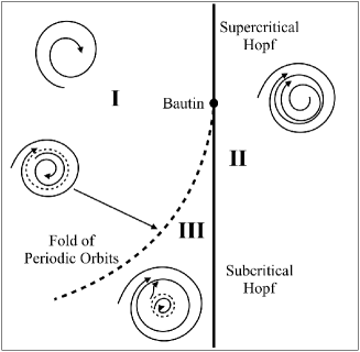
a) b)

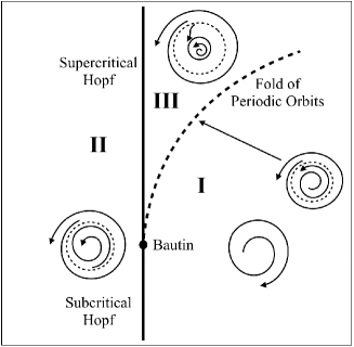
Figure 1: The Bautin bifurcation diagram near the equilibrium for a) $l_{2}(0)<0$ and b) $l_{2}(0)>0$.

3 Example: Segel-Jackson model

In this section, we shall investigate the Bautin bifurcation for the Segel-Jackson model.

$$\left\{\begin{array}[]{l}\frac{\partial u(x,t)}{\partial t}=d\Delta u(x,t)+[1+ku(x,t)]u(x,t)-au(x,t)v(x,t)\\ \frac{\partial v(x,t)}{\partial t}=\Delta v(x,t)+u(x,t-\tau)v(x,t-\tau)-v^{2}(x,t)\end{array}~{}~{}~{}~{}~{}x\in[0,l\pi],t>0\right..$$ (19)

$u(x,t)$ stands for the density of the prey and $v(x,t)$ the predator. $d$ is the diffusion rate of the prey whereas the diffusion rate of predator is normalized by 1. $1+ku(x,t)$ stands for the reproduction rate per capita of prey. $a$ is the ability of the predator hunting the prey.

Equipping (19) with homogeneous Neumann boundary condition $\left.\frac{\partial u}{\partial x}\right|_{x=0,l\pi}=\left.\frac{\partial v}{\partial x}\right|_{x=0,l\pi}=0$, there are two constant equilibria of system (19): one is the trivial equilibrium $E_{0}=(0,0)$ and the other is the unique positive equilibrium $E_{\ast}=(u^{\ast},v^{\ast})=(\frac{1}{a-k},\frac{1}{a-k})$, provided that $k<a$.

The linear equation of system (19) at $E_{\ast}$ is

$$\left\{\begin{array}[]{l}\frac{\partial u(x,t)}{\partial t}=d\Delta u(x,t)+\frac{k}{a-k}u(x,t)+\frac{a}{k-a}v(x,t),\\ \frac{\partial v(x,t)}{\partial t}=\Delta v(x,t)+\frac{2}{k-a}v(x,t)+\frac{1}{a-k}u(x,t-\tau)+\frac{1}{a-k}v(x,t-\tau).\end{array}\right.$$ (20)

Then we have the characteristic equation of system (20) is

$$\lambda^{2}+A_{n}\lambda+B\lambda{{\rm e}}^{-\lambda\tau}+C_{n}+D_{n}{{\rm e}}^{-\lambda\tau}=0,$$ (21)

with $A_{n}=\frac{k-2}{k-a}+\frac{(d+1)n^{2}}{l^{2}}$, $B=\frac{1}{k-a}$, $C_{n}=\left(\frac{k}{a-k}-\frac{dn^{2}}{l^{2}}\right)\left(\frac{2}{k-a}-\frac{n^{2}}{l^{2}}\right)$, $D_{n}=\frac{k+a}{(a-k)^{2}}-\frac{dn^{2}}{(a-k)l^{2}}$.

In the following, we will discuss the stability of $E_{\ast}$, regarding time delay $\tau$ and $k$ as bifurcation parameters.

When $\tau=0$, Eq.(21) becomes

$$\lambda^{2}+(A_{n}+B)\lambda+C_{n}+D_{n}=0.$$ (22)

In fact, this is just the case investigated in Wang , and we state the main results here: when $\tau=0$, assume that

$$k<\min\{1,a,d\}~{}~{}~{}~{}~{}~{}(H_{1})$$

holds true, then the positive equilibrium $E_{\ast}$ is locally asymptotically stable.

In the following part, we will investigate the existence of Hopf bifurcations destabilizing $E_{\ast}$ as $\tau$ increases, where we always assume $(H_{1})$ holds true.

When $\tau>0$, following the method given in wei2 , we plug $\lambda={\rm i}\omega$ into Eq.(21) and separate the real and imaginary parts, then obtain

$$\left\{\begin{array}[]{l}D_{n}\cos\omega\tau+B\omega\sin\omega\tau=\omega^{2}-C_{n},\\ -D_{n}\sin\omega\tau+B\omega\cos\omega\tau=-A_{n}\omega.\end{array}\right.$$ (23)

This is a linear equation about unknowns $\cos\omega\tau$ and $\sin\omega\tau$. Once $\omega$ and $n$ are fixed, we can solve from (23) that $\cos\omega\tau:=\tilde{C}_{n}(\omega)$ and $\sin\omega\tau:=\tilde{S}_{n}(\omega).$

Adding the square of both sides of Eq.(23), we have an algebraic equation about $\omega^{2}$, denoted by

$$(\omega^{2})^{2}+M_{1}\omega^{2}+M_{2}=0$$ (24)

with $M_{1}=-2C_{n}+A_{n}^{2}-B^{2}$ and $M_{2}=C_{n}^{2}-D_{n}^{2}$.

If $M_{1}<0,~{}M_{2}>0,~{}M_{1}^{2}-4M_{2}>0$ hold true, Eq.(24) has two positive roots, given by

$$\omega=\omega_{n}^{\pm}=\sqrt{\frac{-M_{1}\pm\sqrt{M_{1}^{2}-4M_{2}}}{2}}.$$

Else if $M_{2}<0$ holds true, Eq.(24) has only one positive root, denoted by

$$\omega=\omega_{n}^{+}=\sqrt{\frac{-M_{1}+\sqrt{M_{1}^{2}-4M_{2}}}{2}}.$$

Plugging $\omega_{n}^{+}$ or $\omega_{n}^{\pm}$ into Eq.(23), at most two sequences of possible Hopf bifurcation values are obtained, which are denoted by

$$\tau_{n,j}^{\pm}=\left\{\begin{array}[]{ll}\frac{\arccos\tilde{C}_{n}(\omega_{n}^{\pm})+2j\pi}{\omega_{n}^{\pm}},&~{}if~{}\tilde{S}_{n}(\omega_{n}^{\pm})\geq 0\\ \frac{\arcsin\tilde{S}_{n}(\omega_{n}^{\pm})+2\pi+2j\pi}{\omega_{n}^{\pm}},&~{}if~{}\tilde{S}_{n}(\omega_{n}^{\pm})<0~{}and~{}\tilde{C}_{n}(\omega_{n}^{\pm})\geq 0\\ \frac{-\arcsin\tilde{S}_{n}(\omega_{n}^{\pm})+\pi+2j\pi}{\omega_{n}^{\pm}},&~{}if~{}\tilde{S}_{n}(\omega_{n}^{\pm})<0~{}and~{}\tilde{C}_{n}(\omega_{n}^{\pm})<0\end{array}\right.~{}~{}~{}~{}n,j=0,1,2,\cdots.$$ (25)

We know when $\tau=\tau_{n,j}^{\pm},n,j=0,1,2,\cdots$, Eq.(21) has a pair of imaginary roots. By re-scaling time $t\rightarrow t/\tau$, making transformation $\tilde{u}=u(x,t)-u^{\ast},$ $\tilde{v}=v(x,t)-v^{\ast}$ and dropping the tildes for convenience, we have system (19) becomes

$$\left\{\begin{array}[]{l}\frac{\partial u}{\partial t}=\tau\left[d\Delta u+(1+2ku^{\ast}-av^{\ast})u-au^{\ast}v+f_{1}(u_{t},v_{t})\right]\\ \frac{\partial v}{\partial t}=\tau\left[\Delta v-2v^{\ast}v+v^{\ast}u_{t}(-1)+u^{\ast}v_{t}(-1)+f_{2}(u_{t},v_{t})\right]\end{array}\right.$$ (26)

where $u=u(x,t)$, $v=v(x,t)$. For any $(\phi_{1},\phi_{2})\in\mathscr{C}:=C([-1,0],X)$ and $X:=\{(u,v)\in H^{2}(0,l\pi)\times H^{2}(0,l\pi):\frac{du}{dx}=\frac{dv}{dx}=0~{}at~{}x=0,l\pi\}$, two nonlinear functionals are defined by

$$f_{1}(\phi_{1},\phi_{2})=k{\phi_{1}}^{2}(0)-a{\phi_{1}}(0){\phi_{2}}(0)$$ (27)

and

$$f_{2}(\phi_{1},\phi_{2})=-\phi_{2}^{2}(0)+\phi_{1}(-1)\phi_{2}(-1).$$ (28)

We will calculate the first and second Lyapunov coefficients of the normal forms when $\tau=\tau^{\ast}\in\{\tau_{n,j}^{\pm},~{}n,j=0,1,2,\cdots\}$ and for any fixed $k$, while Eq.(21) has a pair of imaginary roots $\lambda=\pm\textrm{i}\omega_{n}^{\pm}$ for $n=n_{0}$. For simplification, we denote $\omega_{n_{0}}^{\pm}$ by $\omega^{\ast}$.

Let $\tau=\tau^{\ast}+\epsilon$. We can rewrite system (26) in an abstract form in the phase space $\mathscr{C}:=C([-1,0],X)$ as

$$\dot{U}(t)=\tilde{D}\Delta U(t)+L_{\epsilon}(U_{t})+F(\epsilon,U_{t})$$ (29)

where  $\tilde{D}=(\tau^{\ast}+\epsilon)D$, $D=\left(\begin{array}[]{cc}d&0\\ 0&1\end{array}\right)$ and $L_{\epsilon}:\mathscr{C}\rightarrow X$, $F:\mathscr{C}\rightarrow X$ are defined, respectively, by

$$L_{\epsilon}(\phi)=(\tau^{\ast}+\epsilon)B_{1}\phi(0)+(\tau^{\ast}+\epsilon)B_{2}\phi(-1)$$

and

$$F(\epsilon,\phi)=(F_{1}(\epsilon,\phi(\theta)),F_{2}(\epsilon,\phi(\theta)))^{\textrm{T}}$$

with

$$B_{1}=\left(\begin{array}[]{cc}1+2ku^{\ast}-av^{\ast}&-au^{\ast}\\ 0&-2v^{\ast}\end{array}\right),~{}~{}B_{2}=\left(\begin{array}[]{cc}0&0\\ v^{\ast}&u^{\ast}\end{array}\right),$$

$$F_{1}(\epsilon,\phi)=(\tau^{\ast}+\epsilon)f_{1}(\phi_{1}(\theta),\phi_{2}(\theta)),~{}~{}~{}for~{}any~{}\phi=(\phi_{1},\phi_{2})\in\mathscr{C}$$ (30)

and

$$F_{2}(\epsilon,\phi)=(\tau^{\ast}+\epsilon)f_{2}(\phi_{1}(\theta),\phi_{2}(\theta)),~{}~{}~{}for~{}any~{}\phi=(\phi_{1},\phi_{2})\in\mathscr{C}.$$ (31)

Thus, the linearized equation of system (26) at the equilibrium $(0,0)$ has the form

$$\dot{U}(t)=\tilde{D}\Delta U(t)+L_{\epsilon}(U_{t}).$$ (32)

We have that the solution operator of system (26) forms a $C_{0}$ semigroup with the infinitesimal generator $A_{\epsilon}$,

$$A_{\epsilon}\phi=\left\{\begin{array}[]{ll}\dot{\phi}(\theta),&\theta\in[-r,0),\\ \tilde{D}\Delta\phi(0)+L_{\epsilon}(\phi),&\theta=0.\end{array}\right.$$ (33)

The domain of $A_{\epsilon}$ is chosen by

$${\rm dom}(A_{\epsilon}):=\{\phi\in\mathscr{C}:\dot{\phi}\in\mathscr{C},\phi(0)\in{\rm dom}(\Delta),\dot{\phi}(0)=\tilde{D}\Delta\phi(0)+L_{\epsilon}(\phi)\}.$$

In order to use the results we obtained in the precious section, in the space $\mathscr{C}$ we rewrite Eq.(29) as the abstract form

$$\dot{U}(t)=A_{\epsilon}U_{t}+R(\epsilon,U_{t})$$ (34)

where the nonlinear term is given by

$$R(\epsilon,U_{t})(\theta)=\left\{\begin{array}[]{ll}0,&\theta\in[-1,0),\\ F(\epsilon,U_{t}),&\theta=0.\end{array}\right.$$

In the state space $X$, we know, $\left(\cos\frac{nx}{l}(0,1)^{\textrm{T}},\cos\frac{nx}{l}(1,0)^{\textrm{T}}\right),~{}~{}n=0,1,2,\cdots,$ are eigenfunctions of $\Delta$ with the no-flux boundary conditions. Moreover, they form a basis of $X$ which are normalized by $b_{n}=\frac{\cos(\frac{nx}{l})}{\|\cos\frac{nx}{l}\|_{L_{2}}}$. For convenience we use $\beta_{n}=\{b_{n}(1,0)^{\textrm{T}},b_{n}(0,1)^{\textrm{T}}\}$ to be the basis of $X$.

Using the notations introduced in Section 2, for any $\phi=(\phi^{(1)},\phi^{(2)})^{\textrm{T}}\in\mathscr{C}$, we denote

$$\phi_{n}=<\phi,\beta_{n}>=\left(<\phi^{(1)},b_{n}>,<\phi^{(2)},b_{n}>\right)^{\textrm{T}}$$

as the coordinates of $\phi$ on $\beta_{n}$ in $X$.

The restriction of $A$, $A_{\epsilon,n}$ is then defined by

$$A_{\epsilon,n}(\phi_{n}(\theta)b_{n})=\left\{\begin{array}[]{ll}\dot{\phi}_{n}(\theta)b_{n},&\theta\in[-1,0),\\ \int_{-1}^{0}d\eta_{n}(\epsilon,\theta)\phi_{n}(\theta)b_{n},&\theta=0,\end{array}\right.$$

with

$$\eta_{n}(\epsilon,\theta)=\left\{\begin{array}[]{ll}-(\tau^{\ast}+\epsilon)B_{2},&\theta=-1,\\ 0,&\theta\in(-1,0),\\ (\tau^{\ast}+\epsilon)(B_{1}-\frac{n^{2}}{l^{2}}D),&\theta=0.\end{array}\right.$$

Similarly, the linear operator $L_{2}$ has the restriction

$$L_{\epsilon,n}(\phi_{n})=(\tau^{\ast}+\epsilon)B_{1}\phi_{n}(0)+(\tau^{\ast}+\epsilon)B_{2}\phi_{n}(-1).$$

Obviously, we have, from the linear Eq.(32)

$$-\frac{n^{2}}{l^{2}}\tilde{D}\phi_{n}(0)+L_{\epsilon,n}(\phi_{n})=\int_{-1}^{0}d\eta_{n}(\epsilon,\theta)\phi_{n}(\theta)b_{n}.$$

Similar as the previous section we can define the adjoint operator $A^{\ast}$ of $A_{0}$ as

$$A^{\ast}\varphi(s)=\left\{\begin{array}[]{ll}-\dot{\varphi}(s),&s\in(0,1],\\ \sum\limits_{n=0}^{\infty}\int_{-1}^{0}d\eta_{n}^{\textrm{T}}(0,t)\varphi_{n}(-t)b_{n},&s=0.\end{array}\right.$$

As we stated at the beginning of this section, we can calculate the eigenfunctions of $A_{0}$ and $A^{\ast}$ at the eigenvalue $\textrm{i}\omega^{\ast}\tau^{\ast}$ and $-\textrm{i}\omega^{\ast}\tau^{\ast}$, which are, respectively, $qb_{n_{0}}$ and $q^{\ast}b_{n_{0}}$.

By direct calculations, we have $q(\theta)=(1,q_{1})^{\textrm{T}}\textrm{e}^{\textrm{i}\omega^{\ast}\tau^{\ast}\theta}$ and $q^{\ast}(s)=M(q_{2},1)^{\textrm{T}}\textrm{e}^{\textrm{i}\omega^{\ast}\tau^{\ast}s}$. Here

$$q_{1}=\frac{1+2ku^{\ast}-av^{\ast}-\frac{dn^{2}}{l^{2}}+\textrm{i}\omega^{\ast}\tau^{\ast}}{au^{\ast}},$$

$$q_{2}=\frac{-2v^{\ast}-\frac{n^{2}}{l^{2}}+\textrm{e}^{\textrm{i}\omega^{\ast}\tau^{\ast}}u^{\ast}+\textrm{i}\omega^{\ast}\tau^{\ast}}{au^{\ast}}$$

and

$$\bar{M}=[{(\bar{q_{2}}+q_{1})+\textrm{e}^{-\textrm{i}\omega^{\ast}\tau^{\ast}}\tau^{\ast}(v^{\ast}+q_{1}u^{\ast})}]^{-1},$$

such that $(q^{\ast},q)_{c}=1$. By the formal adjoint theory, we have $(\bar{q^{\ast}},q)_{c}=(q^{\ast},\bar{q})=0.$ By using the standard theory of phase space decomposition, we have the eigenvalues $\Lambda=\{\pm\textrm{i}\omega^{\ast}\tau^{\ast}\}$ can be used to decompose $\mathscr{C}$ by $\mathscr{C}=P\bigoplus Q$. The center space $P$ is given by

$$P=\{zqb_{n_{0}}+\bar{z}qb_{n_{0}}|z\in\mathbb{C}\}$$

and its orthogonal complement space is

$$Q=\{\phi\in\mathscr{C}|(q^{\ast}b_{n_{0}},\phi)=0~{}and~{}(\bar{q}^{\ast}b_{n_{0}},\phi)=0\}.$$

Thus, the state of system (34) could be decomposed, correspondingly, by

$$U_{t}=z(t)q(\cdot)b_{n_{0}}+\bar{z}(t)\bar{q}(\cdot)b_{n_{0}}+W(t,\cdot)$$

where $W(t,\cdot)\in Q.$

Notice the relation between $q^{\ast}$ and $q$, we calculate $z(t)$ by

$$z(t)=(q^{\ast}b_{n_{0}},U_{t}).$$ (35)

Thus, $W(t,\theta)=U_{t}(\theta)-2{\rm Re}\{z(t)q(\theta)b_{n_{0}}\}$. Then we obtain the reduced equation onto the center space

$$\dot{z}(t)=\textrm{i}\omega_{0}z(t)+\bar{q}^{\ast\textrm{T}}<F(0,U_{t}),\beta_{n_{0}}>,$$ (36)

where the nonlinear term is given by

$$<F,\beta_{n}>:=(<F_{1},b_{n}>,<F_{2},b_{n}>)^{\textrm{T}},$$

with $F_{1}$ and $F_{2}$ already defined in (30) and (31).

Using the center manifold theorem Lin , there exists a center manifold $\mathscr{C}_{0}$ and on $\mathscr{C}_{0}$ we have $W(t,\cdot)$ can be expressed by series

$$\begin{array}[]{ll}W(t,\cdot)&=W(z(t),\bar{z}(t),\cdot)=W_{20}\frac{z^{2}}{2}+W_{11}z\bar{z}+W_{02}\frac{\bar{z}^{2}}{2}+W_{30}\frac{z^{3}}{6}+W_{21}\frac{z^{2}\bar{z}}{2}+W_{12}\frac{z\bar{z}^{2}}{2}\\ &+W_{03}\frac{\bar{z}^{3}}{6}+W_{31}\frac{z^{3}\bar{z}}{6}+W_{22}\frac{z^{2}\bar{z}^{2}}{4}+\cdots.\end{array}$$ (37)

For solution $U_{t}\in\mathscr{C}_{0},$ we have $U_{t}=z(t)q(\cdot)b_{n_{0}}+\bar{z}(t)\bar{q}(\cdot)+W(z(t),\bar{z}(t),\theta)$ and denote by

$$F(0,U_{t})|_{\mathscr{C}_{0}}=\tilde{F}(0,z,\bar{z}).$$

We write the Taylor expression

$$\begin{array}[]{ll}\tilde{F}(0,z,\bar{z})&=\tilde{F}^{\prime\prime}_{zz}\frac{z^{2}}{2}+\tilde{F}^{\prime\prime}_{z\bar{z}}z\bar{z}+\tilde{F}^{\prime\prime}_{\bar{z}\bar{z}}\frac{\bar{z}^{2}}{2}+\tilde{F}^{\prime\prime\prime}_{zzz}\frac{z^{3}}{6}+\tilde{F}^{\prime\prime\prime}_{zz\bar{z}}\frac{z^{2}\bar{z}}{2}+\tilde{F}^{\prime\prime\prime}_{z\bar{z}\bar{z}}\frac{z\bar{z}^{2}}{2}+\tilde{F}^{\prime\prime\prime}_{\bar{z}\bar{z}\bar{z}}\frac{\bar{z}^{3}}{6}\\ &+\tilde{F}^{\prime\prime\prime\prime}_{zzzz}\frac{z^{4}}{24}+\tilde{F}^{\prime\prime\prime\prime}_{zzz\bar{z}}\frac{z^{3}\bar{z}}{6}+\tilde{F}^{\prime\prime\prime\prime}_{zz\bar{z}\bar{z}}\frac{z^{2}\bar{z}^{2}}{4}+\tilde{F}^{\prime\prime\prime\prime}_{z\bar{z}\bar{z}\bar{z}}\frac{z\bar{z}^{3}}{6}+\tilde{F}^{\prime\prime\prime\prime}_{\bar{z}\bar{z}\bar{z}\bar{z}}\frac{\bar{z}^{4}}{24}\\ &+\tilde{F}^{\prime\prime\prime\prime\prime}_{zzz\bar{z}\bar{z}}\frac{z^{3}\bar{z}^{2}}{12}+\cdots.\end{array}$$ (38)

In fact, from Eqs.(27-28) and (30-31), we have

$$\begin{array}[]{l}\tilde{F}^{\prime\prime}_{zz}=\tau^{\ast}\left(\begin{array}[]{c}2k-2aq_{1}\\ -2q_{1}^{2}+2q_{1}{{\rm e}}^{-2{{\rm i}}\omega^{\ast}\tau^{\ast}}\end{array}\right)b_{n_{0}}^{2},\\ \tilde{F}^{\prime\prime}_{\bar{z}\bar{z}}=\tau^{\ast}\left(\begin{array}[]{c}2k-2a\bar{q}_{1}\\ -2\bar{q}_{1}^{2}+2\bar{q}_{1}{{\rm e}}^{2{{\rm i}}\omega^{\ast}\tau^{\ast}}\end{array}\right)b_{n_{0}}^{2},\\ \tilde{F}^{\prime\prime}_{z\bar{z}}=\tau^{\ast}\left(\begin{array}[]{c}2k-a(q_{1}+\bar{q}_{1})\\ -2\bar{q}_{1}q_{1}+(q_{1}+\bar{q}_{1})\end{array}\right)b_{n_{0}}^{2},\end{array}$$ (39)

and all the rest higher-order derivatives are zero.

Now rewrite the equation on the center manifold (36) as

$$\dot{z}(t)=\textrm{i}\omega_{0}z(t)+g(z,\bar{z}).$$ (40)

In order to calculate the normal form, we expand

$$\begin{array}[]{ll}g(z,\bar{z})&=g_{20}\frac{z^{2}}{2}+g_{11}z\bar{z}+g_{02}\frac{\bar{z}^{2}}{2}+g_{21}\frac{z^{2}\bar{z}}{2}+g_{12}\frac{z\bar{z}^{2}}{2}+g_{03}\frac{\bar{z}^{3}}{6}+g_{40}\frac{z^{4}}{24}+g_{31}\frac{z^{3}\bar{z}}{6}+g_{22}\frac{z^{2}\bar{z}^{2}}{4}\\ &+g_{13}\frac{z\bar{z}^{3}}{6}+g_{04}\frac{\bar{z}^{4}}{24}+g_{32}\frac{z^{3}\bar{z}^{2}}{12}+\cdots.\end{array}$$ (41)

By comparing the same order of terms, we obtain the expressions of $g_{ij}$’s, which, together with the detailed derivations, are given in the Appendix.

According to the results given in Section 2, the first and second Lyapunov coefficients can be expressed by

$$l_{1}(k,\tau^{\ast})=\frac{1}{2\omega^{\ast}\tau^{\ast}}\left({\rm Re}g_{21}-\frac{1}{\omega^{\ast}\tau^{\ast}}{{\rm Im}}\{g_{20}g_{11}\}\right)$$ (42)

and

$$\begin{array}[]{rl}&12l_{2}(k,\tau^{\ast})=\frac{1}{\tau^{\ast}\omega^{\ast}}{\rm Re}{g_{32}}\\ &~{}~{}+\frac{1}{(\tau^{\ast}\omega^{\ast})^{2}}{{\rm Im}}\left\{g_{20}\bar{g}_{31}-g_{11}(4g_{31}+3\bar{g}_{22})-\frac{1}{3}g_{02}(g_{40}+\bar{g}_{13})-g_{30}g_{12}\right\}\\ &~{}~{}+\frac{1}{(\tau^{\ast}\omega^{\ast})^{3}}{\rm Re}\left\{g_{20}\left[\bar{g}_{11}(3g_{12}-\bar{g}_{30})+g_{02}\left(\bar{g}_{12}-\frac{1}{3}g_{30}\right)+\frac{1}{3}\bar{g}_{02}g_{03}\right]\right\}\\ &~{}~{}+\frac{1}{(\tau^{\ast}\omega^{\ast})^{3}}{\rm Re}\left\{g_{11}\left[\bar{g}_{02}\left(\frac{5}{3}\bar{g}_{30}+3g_{12}\right)+\frac{1}{3}g_{02}\bar{g}_{03}-4g_{11}g_{30}\right]\right\}\\ &~{}~{}+\frac{3}{(\tau^{\ast}\omega^{\ast})^{3}}{{\rm Im}}\{g_{20}g_{11}\}{{\rm Im}}\{g_{21}\}+\frac{1}{(\tau^{\ast}\omega^{\ast})^{4}}{{\rm Im}}\{g_{11}\bar{g}_{02}[\bar{g}_{20}^{2}-3\bar{g}_{20}g_{11}-4g_{11}^{2}\}\\ &~{}~{}+\frac{1}{(\tau^{\ast}\omega^{\ast})^{4}}{{\rm Im}}\left\{g_{11}g_{20}\right\}[3{\rm Re}\{g_{11}g_{20}\}-2|g_{02}|^{2}].\end{array}$$ (43)

Fixing $a=5$ and $d=1$, we can use the method above to determine the Hopf bifurcation values of $\tau$ for any given $k$. By using the formula (25) , we know at $(k,\tau)=(k^{\ast},\tau^{\ast})=(0.3075,0.6543)$, the characteristic equation (21) has a pair of imaginary roots $\lambda=\pm 0.4233{{\rm i}}$, i.e., $\omega^{\ast}=0.4233$, and all the rest roots have negative real part. Further calculations from Eq.(42) and (43) yield $l_{1}(k^{\ast},\tau^{\ast})=0$ (as shown in Figure 2 (a)) and $l_{2}(k^{\ast},\tau^{\ast})=0.0376>0$.

The transversality condition can be verified, numerically, by

$$\left|\begin{array}[]{cc}\frac{\partial\frac{\alpha(k,\tau)}{\omega(k,\tau)}}{\partial k}&\frac{\partial\frac{\alpha(k,\tau)}{\omega(k,\tau)}}{\partial\tau}\\ \frac{\partial l_{1}(k,\tau)}{\partial k}&\frac{\partial l_{1}(k,\tau)}{\partial\tau}\end{array}\right|_{(k,\tau)={k^{\ast},\tau^{\ast}}}=\left|\begin{array}[]{cc}\frac{\alpha^{\prime}_{k}(k^{\ast},\tau^{\ast})}{\omega(k^{\ast},\tau^{\ast})}&\frac{\alpha^{\prime}_{\tau}(k^{\ast},\tau^{\ast})}{\omega(k^{\ast},\tau^{\ast})}\\ \frac{\partial l_{1}(k,\tau)}{\partial k}&\frac{\partial l_{1}(k,\tau)}{\partial\tau}\end{array}\right|=\left|\begin{array}[]{cc}0.2946&0.3085\\ 1.5728&-1.1954\end{array}\right|=-0.8374\neq 0.$$ (44)

Thus the map $(k,\tau)\mapsto(\frac{\alpha(k,\tau)}{\omega(k\tau)},l_{1}(k,\tau))$ is regular at $(k^{\ast},\tau^{\ast})$, and the system undergoes a Bautin bifurcation at $(k^{\ast},\tau^{\ast})$ with the bifurcation diagram topologically equivalent to Figure 1 (b). When $k<k^{\ast}=0.3075$, the Hopf bifurcation is subcritical, as shown in Figure 3 (a). The Bautin bifurcation diagrams is shown in Figure 2 (b). When $k>k^{\ast}$, the Hopf bifurcation is supercritical. As shown in Figure 3 (b), the fold bifurcation of periodic orbits eliminates the stable and unstable periodic orbits.

In fact, we find that when $k=0.8$ and $\tau\in(0.9566,1.1550)$, solutions with small initial values converge to a stable periodic orbits (Figure 4), and those with large initial values diverge to infinity as time goes to infinity (Figure 5).

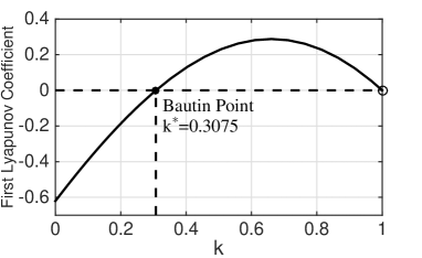
a) b)

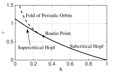
Figure 2: $a=5$. a) the first Lyapunov coefficient $l_{1}$ varies with respect to $k$. b) the Bautin bifurcation diagram near the Bautin point $(k^{\ast},\tau^{\ast})=(0.3075,0.6543)$.

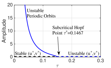
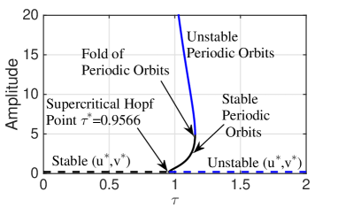
Figure 3: $a=5$. (a) Subcritical bifurcation diagram when $k=0.8$. (b) Supercritical bifurcation diagram when $k=0.1$.

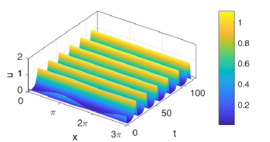
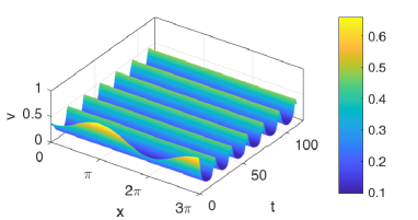
Figure 4: $k=0.1$ $a=5$. For $\tau=1.05$, the solution of (19) with initial value $u_{0}(x,t)=0.3-0.16\cos x$, $v_{0}(x,t)=0.5-0.16\cos x$ converges to a periodic solution.

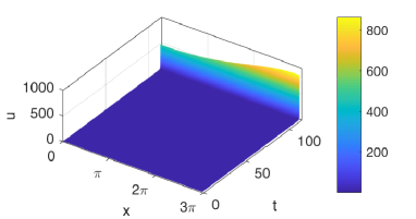
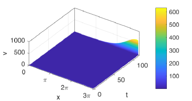
Figure 5: $k=0.1$, $a=5$. For $\tau=1.05$, the solution of (19) with initial value $u_{0}(x,t)=10.3-0.16\cos x$, $v_{0}(x,t)=10.5-0.16\cos x$ diverges to infinity.

Conclusion

In this paper, a universal and explicit method to calculate the first and second Lyapunov coefficients at a pair of imaginary eigenvalues in reaction-diffusion system with time delays is given, which can be used to determine the dynamics near a Bautin bifurcation point. As an example, the method is applied to the Segel-Jackson model. Near the Bautin bifurcation we theoretically proved that solutions with small (large) initial values are convergent to stable periodic oscillations (diverge to infinity).

Appendix

In this Appendix, we will give detailed formulae to calculating $g_{ij}$’s, then the first and second Lyapunov coefficients are determined.

In fact, by comparing the same order of terms, we have

$$g_{20}=2\bar{M}\tau^{\ast}\left[\bar{q_{2}}(k-aq_{1})+(-q_{2}^{2}+q_{1}\textrm{e}^{-2\textrm{i}\omega^{\ast}\tau^{\ast}})\right]\int_{0}^{l\pi}b_{n_{0}}^{3}dx,$$

$$g_{11}=\bar{M}\tau^{\ast}\{\bar{q_{2}}[2k-a(\bar{q_{1}}q_{1})]-2q_{1}\bar{q_{1}}+\bar{q_{1}}+q_{1}\}\int_{0}^{l\pi}b_{n_{0}}^{3}dx,$$

$$g_{02}=2\bar{M}\tau^{\ast}\left[\bar{q_{2}}(k-a\bar{q_{1}})+(-\bar{q_{2}}^{2}+\bar{q_{1}}\textrm{e}^{2\textrm{i}\omega^{\ast}\tau^{\ast}})\right]\int_{0}^{l\pi}b_{n_{0}}^{3}dx,$$

$$g_{30}=3\bar{M}\tau^{\ast}\int_{0}^{l\pi}\left\{\bar{q_{2}}(k+1)W_{20}^{(1)}(0)-q_{1}\left[W_{20}^{(1)}(0)+W_{20}^{(2)}(0)\right]+2W_{20}^{(1)}(-1)\right\}b_{n_{0}}^{2}dx,$$

$$\begin{array}[]{ll}g_{21}=&\bar{M}\tau^{\ast}\bar{q_{2}}\int_{0}^{l\pi}\left\{2k\left[W_{11}^{(1)}(0)+W_{20}^{(1)}(0)\right]\right.\\ &\left.-a\left[2W_{11}^{(2)}(0)+W_{20}^{(2)}(0)+\bar{q_{1}}W_{20}^{(1)}(0)+2q_{1}W_{11}^{(1)}(0)\right]\right\}b_{n_{0}}^{2}dx\\ &+\frac{1}{2}\bar{M}\tau^{\ast}\int_{0}^{l\pi}\left\{-\left[8q_{1}W_{11}^{(2)}(0)+2\bar{q}_{1}W_{20}^{(2)}(0)+W_{20}^{(2)}(0)W_{02}^{(2)}(0)\right]+\left[4\textrm{e}^{-\textrm{i}\omega^{\ast}\tau^{\ast}}W_{11}^{(2)}(-1)\right.\right.\\ &\left.\left.+2\textrm{e}^{\textrm{i}\omega^{\ast}\tau^{\ast}}W_{20}^{(2)}(-1)+2\textrm{e}^{\textrm{i}\omega^{\ast}\tau^{\ast}}\bar{q}_{1}W_{20}^{(1)}(-1)+4\textrm{e}^{-\textrm{i}\omega^{\ast}\tau^{\ast}}q_{1}W_{11}^{(1)}(-1)\right]\right\}b_{n_{0}}^{2}dx,\end{array}$$

$$\begin{array}[]{ll}g_{12}=&\bar{M}\tau^{\ast}\bar{q_{2}}\int_{0}^{l\pi}\left\{k\left[3W_{02}^{(1)}(0)+4W_{11}^{(1)}(0)\right]\right.\\ &\left.-a\left[2W_{11}^{(2)}(0)+W_{02}^{(2)}(0)+{q_{1}}W_{02}^{(1)}(0)+2\bar{q}_{1}W_{11}^{(1)}(0)\right]\right\}b_{n_{0}}^{2}dx\\ &+\bar{M}\tau^{\ast}\int_{0}^{l\pi}\left\{-\left[(q_{1}+\bar{q}_{1}W_{20}^{(2)}(0)+2(\bar{q}_{1}+1)W_{11}^{(2)}(0)+q_{1}W_{02}^{(2)}(0)\right]+\left[\textrm{e}^{-\textrm{i}\omega^{\ast}\tau^{\ast}}W_{02}^{(2)}(-1)\right.\right.\\ &\left.\left.+2\textrm{e}^{\textrm{i}\omega^{\ast}\tau^{\ast}}W_{11}^{(2)}(-1)+2\bar{q}_{1}\textrm{e}^{\textrm{i}\omega^{\ast}\tau^{\ast}}W_{11}^{(1)}(-1)+\textrm{e}^{-\textrm{i}\omega^{\ast}\tau^{\ast}}q_{1}W_{02}^{(1)}(-1)\right]\right\}b_{n_{0}}^{2}dx,\end{array}$$

$$\begin{array}[]{ll}g_{03}=&3\bar{M}\tau^{\ast}\int_{0}^{l\pi}\left\{2\bar{q}_{2}kW_{20}^{(1)}(0)-a\bar{q}_{2}\left[W_{02}^{(2)}(0)+\bar{q}_{1}W_{02}^{(1)}(0)\right]-2\bar{q}_{1}W_{02}^{(2)}(0)\right.\\ &+\left.\textrm{e}^{-\textrm{i}\omega^{\ast}\tau^{\ast}}\left[W_{02}^{(2)}(-1)+\bar{q}_{1}W_{02}^{(1)}(-1)\right]\right\}b_{n_{0}}^{2}dx,\end{array}$$

$$\begin{array}[]{ll}g_{40}=&2\bar{M}\tau^{\ast}\bar{q}_{2}\left\{k\left[4\int_{0}^{l\pi}W_{30}^{(1)}(0)b_{n_{0}}^{2}dx+3\int_{0}^{l\pi}\left(W_{20}^{(1)}(0)\right)^{2}b_{n_{0}}dx\right]\right.\\ &\left.-2a\int_{0}^{l\pi}\left[W_{30}^{(2)}(0)+q_{1}W_{30}^{(1)}(0)\right]b_{n_{0}}^{2}dx-3a\int_{0}^{l\pi}W_{20}^{(1)}(0)W_{20}^{(2)}(0)b_{n_{0}}dx\right\}\\ &+2\bar{M}\tau^{\ast}\left\{-\left[4q_{1}\int_{0}^{l\pi}W_{30}^{(2)}(0)b_{n_{0}}^{2}dx+3\int_{0}^{l\pi}\left[2\left(W_{20}^{(2)}(0)\right)^{2}+W_{20}^{(1)}(-1)W_{20}^{(2)}(-1)\right]b_{n_{0}}dx\right]\right.\\ &\left.+2\textrm{e}^{-\textrm{i}\omega^{\ast}\tau^{\ast}}\int_{0}^{l\pi}\left[W_{30}^{(2)}(-1)+q_{1}W_{30}^{(1)}(-1)\right]b_{n_{0}}^{2}dx\right\},\end{array}$$

$$\begin{array}[]{ll}g_{31}=&\bar{M}\tau^{\ast}\bar{q}_{2}\left\{k\int_{0}^{l\pi}\left[9W_{21}^{(1)}(0)+W_{30}^{(1)}(0)\right]b_{n_{0}}^{2}dx+\int_{0}^{l\pi}\left[k-3aW_{20}^{(2)}(0)\right]W_{20}^{(1)}(0)W_{11}^{(1)}(0)b_{n_{0}}dx\right.\\ &\left.-a\int_{0}^{l\pi}\left[3W_{21}^{(2)}(0)+W_{30}^{(2)}(0)+\bar{q}_{1}W_{30}^{(1)}(0)+3q_{1}W_{21}^{(1)}(0)\right]b_{n_{0}}^{2}dx\right\}\\ &+\bar{M}\tau^{\ast}\left\{-\int_{0}^{l\pi}\left[3q_{1}W_{21}^{(2)}(0)+2\bar{q}_{1}W_{30}^{(2)}(0)\right]b_{n_{0}}^{2}dx\right.\\ &\left.-\int_{0}^{l\pi}\left[W_{20}^{(2)}(0)W_{11}^{(2)}(0)-W_{20}^{(1)}(-1)W_{11}^{(2)}(-1)\right]b_{n_{0}}dx\right.\\ &\left.+3\textrm{e}^{-\textrm{i}\omega^{\ast}\tau^{\ast}}\int_{0}^{l\pi}\left[W_{21}^{(2)}(-1)+q_{1}W_{21}^{(1)}(-1)\right]b_{n_{0}}^{2}dx\right.\\ &\left.+\textrm{e}^{\textrm{i}\omega^{\ast}\tau^{\ast}}\int_{0}^{l\pi}\left[W_{30}^{(2)}(-1)+\bar{q}_{1}W_{31}^{(1)}(-1)\right]b_{n_{0}}^{2}dx\right\},\end{array}$$

$$\begin{array}[]{ll}g_{22}=&\bar{M}\tau^{\ast}\bar{q}_{2}\left\{4k\int_{0}^{l\pi}\left[W_{12}^{(1)}(0)+W_{21}^{(1)}(0)\right]b_{n_{0}}^{2}dx+k\int_{0}^{l\pi}\left[2W_{20}^{(1)}(0)W_{02}^{(1)}(0)+\left(W_{11}^{(1)}(0)\right)^{2}\right]b_{n_{0}}dx\right.\\ &\left.-2a\int_{0}^{l\pi}\left[W_{12}^{(2)}(0)+W_{20}^{(2)}(0)+\bar{q}_{1}W_{21}^{(1)}(0)+q_{1}W_{12}^{(1)}(0)\right]b_{n_{0}}^{2}dx\right.\\ &\left.-a\int_{0}^{l\pi}\left[W_{20}^{(1)}(0)W_{02}^{(2)}(0)+4W_{11}^{(1)}(0)W_{11}^{(2)}(0)+W_{02}^{(1)}(0)W_{20}^{(2)}(0)\right]b_{n_{0}}dx\right\}\\ &+\bar{M}\tau^{\ast}\left\{-4\int_{0}^{l\pi}\left[q_{1}W_{12}^{(2)}(0)+\bar{q}_{1}W_{21}^{(2)}(0)\right]b_{n_{0}}^{2}dx+4\left(\textrm{e}^{-\textrm{i}\omega^{\ast}\tau^{\ast}}+\textrm{e}^{\textrm{i}\omega^{\ast}\tau^{\ast}}\right)\int_{0}^{l\pi}W_{21}^{(2)}(-1)b_{n_{0}}^{2}dx\right.\\ &\left.-\int_{0}^{l\pi}\left[W_{20}^{(2)}(0)W_{02}^{(2)}(0)+\left(W_{11}^{(2)}(0)\right)^{2}-W_{11}^{(1)}(-1)W_{11}^{(2)}(-1)\right]b_{n_{0}}dx\right.\\ &\left.+2\int_{0}^{l\pi}\left[\bar{q}_{1}\textrm{e}^{\textrm{i}\omega^{\ast}\tau^{\ast}}W_{21}^{(1)}(-1)+q_{1}\textrm{e}^{-\textrm{i}\omega^{\ast}\tau^{\ast}}W_{12}^{(1)}(-1)\right]b_{n_{0}}^{2}dx\right.\\ &\left.+\int_{0}^{l\pi}W_{22}^{(2)}(-1)\left[W_{20}^{(1)}(-1)+W_{02}^{(1)}(-1)\right]b_{n_{0}}dx\right\},\end{array}$$

$$\begin{array}[]{ll}g_{13}=&\bar{M}\tau^{\ast}\bar{q}_{2}\left\{2k\int_{0}^{l\pi}\left[W_{03}^{(1)}(0)+3W_{12}^{(1)}(0)\right]b_{n_{0}}^{2}dx+k\int_{0}^{l\pi}W_{02}^{(1)}(0)W_{11}^{(1)}(0)b_{n_{0}}dx\right.\\ &\left.-a\int_{0}^{l\pi}\left[3W_{12}^{(2)}(0)+W_{03}^{(2)}(0)+q_{1}W_{03}^{(1)}(0)+3\bar{q}_{1}W_{12}^{(1)}(0)\right]b_{n_{0}}^{2}dx\right.\\ &\left.-3a\int_{0}^{l\pi}\left[W_{11}^{(1)}(0)W_{02}^{2)}(0)+W_{02}^{(1)}(0)W_{11}^{(2)}(0)\right]b_{n_{0}}dx\right\}\\ &+\bar{M}\tau^{\ast}\left\{-2\int_{0}^{l\pi}\left[q_{1}W_{03}^{2)}(0)+3\bar{q}_{1}W_{12}^{2)}(0)\right]b_{n_{0}}^{2}dx\right.\\ &\left.+\textrm{e}^{-\textrm{i}\omega^{\ast}\tau^{\ast}}\int_{0}^{l\pi}\left[W_{03}^{(2)}(-1)+q_{1}W_{03}^{(1)}(-1)\right]b_{n_{0}}^{2}dx\right.\\ &\left.+3\textrm{e}^{\textrm{i}\omega^{\ast}\tau^{\ast}}\int_{0}^{l\pi}\left[W_{12}^{(2)}(-1)+\bar{q}_{1}W_{12}^{(1)}(-1)\right]b_{n_{0}}^{2}dx\right.\\ &\left.+3\int_{0}^{l\pi}W_{02}^{(1)}(-1)W_{11}^{(2)}(-1)b_{n_{0}}dx\right\},\end{array}$$

$$\begin{array}[]{ll}g_{04}=&2\bar{M}\tau^{\ast}\bar{q}_{2}\left\{\int_{0}^{l\pi}\left[(14k-2a\bar{q}_{1})W_{03}^{(1)}(0)-2aW_{03}^{(2)}(0)\right]b_{n_{0}}^{2}dx\right.\\ &\left.+3(k-a)\int_{0}^{l\pi}W_{02}^{(1)}(0)\left[W_{02}^{(1)}(0)+W_{02}^{(2)}(0)\right]b_{n_{0}}dx\right\}\\ &+2\bar{M}\tau^{\ast}\left\{-4\bar{q}_{1}\int_{0}^{l\pi}W_{03}^{(2)}(0)b_{n_{0}}^{2}dx+2\textrm{e}^{\textrm{i}\omega^{\ast}\tau^{\ast}}\int_{0}^{l\pi}\left[W_{03}^{(2)}(-1)+\bar{q}_{1}W_{03}^{(1)}(-1)\right]b_{n_{0}}^{2}dx\right.\\ &\left.-3\int_{0}^{l\pi}\left[\left(W_{02}^{(2)}(0)\right)^{2}-W_{02}^{(1)}(-1)W_{02}^{(2)}(-1)\right]b_{n_{0}}dx\right\}\end{array}$$

and

$$\begin{array}[]{ll}g_{32}=&\bar{M}\tau^{\ast}\bar{q}_{2}\left\{2k\int_{0}^{l\pi}\left[3W_{22}^{(1)}(0)+2W_{31}^{(1)}(0)\right]b_{n_{0}}^{2}dx\right.\\ &\left.+k\int_{0}^{l\pi}\left[9W_{20}^{(1)}(0)W_{12}^{(1)}(0)+12W_{11}^{(1)}(0)W_{21}^{(1)}(0)+2W_{02}^{(1)}(0)W_{30}^{(1)}(0)\right]b_{n_{0}}dx\right.\\ &\left.-a\int_{0}^{l\pi}\left[3W_{22}^{(2)}(0)+2W_{31}^{(2)}(0)+2\bar{q}_{1}W_{31}^{(1)}(0)+3q_{1}W_{21}^{(1)}(0)\right]b_{n_{0}}^{2}dx\right.\\ &\left.-a\int_{0}^{l\pi}\left[3W_{20}^{(1)}(0)W_{12}^{(2)}(0)+6W_{11}^{(1)}(0)W_{21}^{(2)}(0)+W_{02}^{(1)}(0)W_{30}^{(2)}(0)\right.\right.\\ &\left.\left.+W_{30}^{(1)}(0)W_{02}^{(2)}(0)+6W_{21}^{(1)}(0)W_{11}^{(2)}(0)+3W_{12}^{(1)}(0)W_{20}^{(2)}(0)\right]b_{n_{0}}dx\right\}\\ &+2\bar{M}\tau^{\ast}\left\{-2\int_{0}^{l\pi}\left[3q_{1}W_{22}^{(2)}(0)+2\bar{q}_{1}W_{31}^{(2)}(0)\right]b_{n_{0}}^{2}dx\right.\\ &\left.-\int_{0}^{l\pi}\left[12W_{11}^{(2)}(0)W_{21}^{(2)}(0)+2W_{02}^{(2)}(0)W_{30}^{(2)}(0)+3W_{12}^{(2)}(0)W_{20}^{(2)}(0)\right]b_{n_{0}}dx\right.\\ &\left.+3\textrm{e}^{-\textrm{i}\omega^{\ast}\tau^{\ast}}\int_{0}^{l\pi}\left[W_{22}^{(2)}(-1)+q_{1}W_{22}^{(1)}(-1)\right]b_{n_{0}}^{2}dx\right.\\ &\left.+2\textrm{e}^{\textrm{i}\omega^{\ast}\tau^{\ast}}\int_{0}^{l\pi}\left[W_{31}^{(2)}(-1)+\bar{q}_{1}W_{31}^{(1)}(-1)\right]b_{n_{0}}^{2}dx\right.\\ &\left.+\int_{0}^{l\pi}\left[3W_{20}^{(1)}(-1)W_{12}^{(2)}(-1)+W_{02}^{(1)}(-1)W_{30}^{(2)}(-1)\right.\right.\\ &\left.\left.+W_{30}^{(1)}(-1)W_{02}^{(2)}(-1)+6W_{21}^{(1)}(-1)W_{11}^{(2)}(-1)\right]b_{n_{0}}dx\right\}.\end{array}$$

In the current step, we still need to calculate $W_{ij}(\theta)$. Express $H(z,\bar{z},\theta)$ by the Taylor series, we have

$$H(z,\bar{z},\cdot)=H_{20}\frac{z^{2}}{2}+H_{11}z\bar{z}+H_{02}\frac{\bar{z}^{2}}{2}+H_{30}\frac{z^{3}}{6}+H_{21}\frac{z^{2}\bar{z}}{2}+H_{12}\frac{z\bar{z}^{2}}{2}+H_{03}\frac{\bar{z}^{3}}{6}+H_{31}\frac{z^{3}\bar{z}}{6}+H_{22}\frac{z^{2}\bar{z}^{2}}{4}+\cdots.$$

Obviously

$$H_{ij}(\theta)=\left\{\begin{array}[]{ll}-g_{ij}q(\theta)b_{n_{0}}-\bar{g}_{ji}\bar{q}(0)b_{n_{0}},&\theta\in[-r,0),\\ -g_{ij}q(0)b_{n_{0}}-\bar{g}_{ji}\bar{q}(0)b_{n_{0}}+\frac{\partial^{(i+j)}\tilde{F}}{\partial^{i}z\partial^{j}\bar{z}},&\theta=0.\end{array}\right.$$

Notice the definition of $A_{0}$ and Eq.(18), then we have

$$\begin{array}[]{l}(A_{0}-2{\rm i}\omega^{\ast}\tau^{\ast}I)W_{20}(\theta)=-H_{20}(\theta),~{}A_{0}W_{11}(\theta)=-H_{11}(\theta),\\ (A_{0}+2{\rm i}\omega^{\ast}\tau^{\ast}I)W_{02}(\theta)=-H_{02}(\theta),\\ (A_{0}-3{\rm i}\omega^{\ast}\tau^{\ast}I)W_{30}(\theta)-3g_{20}W_{20}(\theta)-3\bar{g}_{02}W_{11}(\theta)=-H_{30}(\theta),\\ (A_{0}-{\rm i}\omega^{\ast}\tau^{\ast}I)W_{21}(\theta)-(g_{20}+2\bar{g}_{11})W_{11}(\theta)-2g_{11}W_{20}(\theta)-\bar{g}_{02}W_{02}(\theta)=-H_{21}(\theta),\\ (A_{0}+{\rm i}\omega^{\ast}\tau^{\ast}I)W_{12}(\theta)-(\bar{g}_{20}+2g_{11})W_{11}(\theta)-2\bar{g}_{11}W_{02}(\theta)-g_{02}W_{20}(\theta)=-H_{12}(\theta),\\ (A_{0}+3{\rm i}\omega^{\ast}\tau^{\ast}I)W_{30}(\theta)-3g_{02}W_{11}(\theta)-3\bar{g}_{20}W_{02}(\theta)=-H_{03}(\theta),\\ (A_{0}-2{\rm i}\omega^{\ast}\tau^{\ast}I)W_{31}(\theta)-3(g_{20}+\bar{g}_{11})W_{21}(\theta)-(g_{30}+3\bar{g}_{12})W_{11}(\theta)-3g_{11}W_{30}(\theta)\\ ~{}~{}~{}~{}-3g_{21}W_{20}(\theta)-\bar{g}_{03}W_{02}(\theta)-3\bar{g}_{02}W_{12}(\theta)=-H_{31}(\theta),\\ A_{0}W_{22}(\theta)-g_{02}W_{30}(\theta)-(g_{20}+4\bar{g}_{11})W_{12}(\theta)-2(g_{21}+\bar{g}_{21})W_{11}(\theta)-2g_{12}W_{20}(\theta)\\ ~{}~{}~{}~{}-(\bar{g}_{20}+4g_{11})W_{21}(\theta)-2\bar{g}_{12}W_{02}(\theta)-\bar{g}_{02}W_{03}(\theta)=-H_{22}(\theta).\end{array}$$ (45)

Similar with the results given in Xu1 , we can solve these functions by

$$W_{20}(\theta)=\frac{{\rm i}g_{20}}{\omega^{\ast}\tau^{\ast}}q(0)b_{n_{0}}{\rm e}^{{\rm i}\omega^{\ast}\tau^{\ast}\theta}+\frac{{\rm i}\bar{g}_{20}}{3\omega^{\ast}\tau^{\ast}}\bar{q}(0)b_{n_{0}}{\rm e}^{-{\rm i}\omega^{\ast}\tau^{\ast}\theta}+T_{1}{\rm e}^{2{\rm i}\omega^{\ast}\tau^{\ast}\theta},$$

$$W_{11}(\theta)=-\frac{{\rm i}g_{11}}{\omega^{\ast}\tau^{\ast}}q(0)b_{n_{0}}{\rm e}^{{\rm i}\omega^{\ast}\tau^{\ast}\theta}+\frac{{\rm i}\bar{g}_{11}}{\omega^{\ast}\tau^{\ast}}\bar{q}(0)b_{n_{0}}{\rm e}^{-{\rm i}\omega^{\ast}\tau^{\ast}\theta}+T_{2},$$

$$W_{02}(\theta)=-\frac{{\rm i}\bar{g}_{20}}{\omega^{\ast}\tau^{\ast}}\bar{q}(0)b_{n_{0}}{\rm e}^{-{\rm i}\omega^{\ast}\tau^{\ast}\theta}-\frac{{\rm i}g_{02}}{3\omega^{\ast}\tau^{\ast}}q(0)b_{n_{0}}{\rm e}^{{\rm i}\omega^{\ast}\tau^{\ast}\theta}+T_{3}{\rm e}^{-2{\rm i}\omega^{\ast}\tau^{\ast}\theta},$$

$$W_{30}(\theta)=\frac{{\rm i}S_{30}^{(1)}}{2\omega^{\ast}\tau^{\ast}}q(0)b_{n_{0}}{\rm e}^{{\rm i}\omega^{\ast}\tau^{\ast}\theta}+\frac{{\rm i}S_{30}^{(2)}}{4\omega^{\ast}\tau^{\ast}}\bar{q}(0)b_{n_{0}}{\rm e}^{-{\rm i}\omega^{\ast}\tau^{\ast}\theta}+\frac{{\rm i}S_{30}^{(3)}}{\omega^{\ast}\tau^{\ast}}\bar{q}(0)b_{n_{0}}{\rm e}^{2{\rm i}\omega^{\ast}\tau^{\ast}\theta}+\frac{{\rm i}S_{30}^{(4)}}{3\omega^{\ast}\tau^{\ast}}+T_{4}{\rm e}^{3{\rm i}\omega^{\ast}\tau^{\ast}\theta},$$

$$W_{21}(\theta)=S_{21}^{(1)}q(0)b_{n_{0}}\theta{\rm e}^{{\rm i}\omega^{\ast}\tau^{\ast}\theta}+\frac{{\rm i}S_{21}^{(2)}}{2\omega^{\ast}\tau^{\ast}}\bar{q}(0)b_{n_{0}}{\rm e}^{-{\rm i}\omega^{\ast}\tau^{\ast}\theta}-\frac{{\rm i}S_{21}^{(3)}}{\omega^{\ast}\tau^{\ast}}{\rm e}^{2{\rm i}\omega^{\ast}\tau^{\ast}\theta}+\frac{{\rm i}S_{21}^{(4)}}{3\omega^{\ast}\tau^{\ast}}{\rm e}^{-2{\rm i}\omega^{\ast}\tau^{\ast}\theta}+\frac{{\rm i}S_{21}^{(5)}}{\omega^{\ast}\tau^{\ast}}+T_{5}{\rm e}^{{\rm i}\omega^{\ast}\tau^{\ast}\theta},$$

$$W_{12}(\theta)=-\frac{{\rm i}S_{12}^{(1)}}{2\omega^{\ast}\tau^{\ast}}q(0)b_{n_{0}}{\rm e}^{{\rm i}\omega^{\ast}\tau^{\ast}\theta}+S_{12}^{(2)}\bar{q}(0)b_{n_{0}}\theta{\rm e}^{-{\rm i}\omega^{\ast}\tau^{\ast}\theta}-\frac{{\rm i}S_{12}^{(3)}}{3\omega^{\ast}\tau^{\ast}}{\rm e}^{2{\rm i}\omega^{\ast}\tau^{\ast}\theta}+\frac{{\rm i}S_{12}^{(4)}}{\omega^{\ast}\tau^{\ast}}{\rm e}^{-2{\rm i}\omega^{\ast}\tau^{\ast}\theta}-\frac{{\rm i}S_{12}^{(5)}}{\omega^{\ast}\tau^{\ast}}+T_{6}{\rm e}^{-{\rm i}\omega^{\ast}\tau^{\ast}\theta},$$

$$W_{03}(\theta)=-\frac{{\rm i}S_{03}^{(1)}}{4\omega^{\ast}\tau^{\ast}}q(0)b_{n_{0}}{\rm e}^{{\rm i}\omega^{\ast}\tau^{\ast}\theta}-\frac{{\rm i}S_{03}^{(2)}}{2\omega^{\ast}\tau^{\ast}}\bar{q}(0)b_{n_{0}}{\rm e}^{-{\rm i}\omega^{\ast}\tau^{\ast}\theta}-\frac{{\rm i}S_{03}^{(3)}}{\omega^{\ast}\tau^{\ast}}{\rm e}^{-2{\rm i}\omega^{\ast}\tau^{\ast}\theta}-\frac{{\rm i}S_{03}^{(4)}}{3\omega^{\ast}\tau^{\ast}}+T_{7}{\rm e}^{-3{\rm i}\omega^{\ast}\tau^{\ast}\theta},$$

$$\begin{array}[]{l}W_{31}(\theta)=\frac{{\rm i}S_{31}^{(1)}}{\omega^{\ast}\tau^{\ast}}{\rm e}^{{\rm i}\omega^{\ast}\tau^{\ast}\theta}+\frac{S_{31}^{(11)}}{(\omega^{\ast}\tau^{\ast})^{2}}{\rm e}^{{\rm i}\omega^{\ast}\tau^{\ast}\theta}+\frac{{\rm i}S_{31}^{(11)}}{\omega^{\ast}\tau^{\ast}}\theta{\rm e}^{{\rm i}\omega^{\ast}\tau^{\ast}\theta}+\frac{{\rm i}S_{31}^{(2)}}{3\omega^{\ast}\tau^{\ast}}{\rm e}^{-{\rm i}\omega^{\ast}\tau^{\ast}\theta}+\frac{S_{31}^{(21)}}{9(\omega^{\ast}\tau^{\ast})^{2}}{\rm e}^{-{\rm i}\omega^{\ast}\tau^{\ast}\theta}\\ +\frac{{\rm i}S_{31}^{(21)}}{3\omega^{\ast}\tau^{\ast}}\theta{\rm e}^{-{\rm i}\omega^{\ast}\tau^{\ast}\theta}+S_{31}^{(3)}\theta{\rm e}^{2{\rm i}\omega^{\ast}\tau^{\ast}\theta}+\frac{{\rm i}S_{31}^{(4)}}{4\omega^{\ast}\tau^{\ast}}{\rm e}^{-2{\rm i}\omega^{\ast}\tau^{\ast}\theta}-\frac{{\rm i}S_{31}^{(5)}}{\omega^{\ast}\tau^{\ast}}{\rm e}^{3{\rm i}\omega^{\ast}\tau^{\ast}\theta}+\frac{{\rm i}S_{31}^{(6)}}{2\omega^{\ast}\tau^{\ast}}+T_{8}{\rm e}^{2{\rm i}\omega^{\ast}\tau^{\ast}\theta}\end{array}$$

and

$$\begin{array}[]{l}W_{22}(\theta)=-\frac{{\rm i}S_{22}^{(1)}}{\omega^{\ast}\tau^{\ast}}{\rm e}^{{\rm i}\omega^{\ast}\tau^{\ast}\theta}-\frac{S_{22}^{(11)}}{\omega^{\ast}\tau^{\ast}}\theta{\rm e}^{{\rm i}\omega^{\ast}\tau^{\ast}\theta}+\frac{{\rm i}S_{22}^{(11)}}{(\omega^{\ast}\tau^{\ast})^{2}}{\rm e}^{{\rm i}\omega^{\ast}\tau^{\ast}\theta}+\frac{{\rm i}S_{22}^{(2)}}{\omega^{\ast}\tau^{\ast}}{\rm e}^{-{\rm i}\omega^{\ast}\tau^{\ast}\theta}+\frac{S_{22}^{(21)}}{\omega^{\ast}\tau^{\ast}}\theta{\rm e}^{-{\rm i}\omega^{\ast}\tau^{\ast}\theta}\\ +\frac{{\rm i}S_{22}^{(21)}}{(\omega^{\ast}\tau^{\ast})^{2}}{\rm e}^{-{\rm i}\omega^{\ast}\tau^{\ast}\theta}-\frac{{\rm i}S_{22}^{(3)}}{2\omega^{\ast}\tau^{\ast}}{\rm e}^{2{\rm i}\omega^{\ast}\tau^{\ast}\theta}+\frac{{\rm i}S_{22}^{(4)}}{2\omega^{\ast}\tau^{\ast}}{\rm e}^{-2{\rm i}\omega^{\ast}\tau^{\ast}\theta}-\frac{{\rm i}S_{22}^{(5)}}{3\omega^{\ast}\tau^{\ast}}{\rm e}^{3{\rm i}\omega^{\ast}\tau^{\ast}\theta}+\frac{{\rm i}S_{22}^{(6)}}{3\omega^{\ast}\tau^{\ast}}{\rm e}^{-3{\rm i}\omega^{\ast}\tau^{\ast}\theta}+S_{22}^{(7)}\theta+T_{9}.\end{array}$$

The coefficients with form $S_{ij}^{(k)}$’s are given by

$$S_{30}^{(1)}=3\frac{{\rm i}g_{20}^{2}}{\omega^{\ast}\tau^{\ast}}+3\frac{{\rm i}g_{20}\bar{g}_{02}}{\omega^{\ast}\tau^{\ast}}+g_{30},~{}S_{30}^{(2)}=\frac{{\rm i}\bar{g}_{02}g_{20}}{\omega^{\ast}\tau^{\ast}}+3\frac{{\rm i}\bar{g}_{11}\bar{g}_{02}}{\omega^{\ast}\tau^{\ast}}+\bar{g}_{03},~{}S_{30}^{(3)}=3g_{20}T_{1},~{}S{30}^{(4)}=3\bar{g}_{02}T_{2},$$

$$S_{21}^{(1)}=-(g_{20}+2\bar{g}_{11})\frac{{\rm i}g_{11}}{\tau^{\ast}\omega^{\ast}}+2g_{11}\frac{{\rm i}g_{20}}{\tau^{\ast}\omega^{\ast}}-\frac{{\rm i}g_{02}\bar{g}_{02}}{3\tau^{\ast}\omega^{\ast}}+g_{21},$$

$$S_{21}^{(2)}=(g_{20}+2\bar{g}_{11})\frac{{\rm i}\bar{g}_{11}}{\tau^{\ast}\omega^{\ast}}+2g_{11}\frac{{\rm i}\bar{g}_{02}}{3\tau^{\ast}\omega^{\ast}}-\frac{{\rm i}\bar{g}_{20}\bar{g}_{02}}{\tau^{\ast}\omega^{\ast}}+\bar{g}_{12},$$

$$S_{21}^{(3)}=2g_{11}T_{1},S_{21}^{(4)}=\bar{g}_{02}T_{3},S_{21}^{(5)}=(g_{02}+2\bar{g}_{11})T_{2},$$

$$S_{12}^{(1)}=\frac{{\rm i}g_{20}g_{02}}{\omega^{\ast}\tau^{\ast}}-(2g_{11}+\bar{g}_{20})\frac{{\rm i}g_{11}}{\omega^{\ast}\tau^{\ast}}-2\bar{g}_{11}\frac{{\rm i}g_{02}}{3\omega^{\ast}\tau^{\ast}}+g_{12},$$

$$S_{12}^{(2)}=\frac{{\rm i}\bar{g}_{02}g_{02}}{3\omega^{\ast}\tau^{\ast}}+(2g_{11}+\bar{g}_{20})\frac{{\rm i}g_{11}}{\omega^{\ast}\tau^{\ast}}-2\frac{{\rm i}\bar{g}_{20}\bar{g}_{11}}{\omega^{\ast}\tau^{\ast}}+\bar{g}_{21},$$

$$S_{12}^{(3)}=g_{02}T_{1},S_{12}^{(4)}=2\bar{g}_{11}T_{3},S_{12}^{(5)}=(2g_{11}+2\bar{g}_{20})T_{2},$$

$$S_{03}^{(1)}=-3\frac{{\rm i}g_{11}g_{02}}{\omega^{\ast}\tau^{\ast}}-\frac{{\rm i}g_{02}\bar{g}_{20}}{\omega^{\ast}\tau^{\ast}}+g_{03},~{}S_{03}^{(2)}=3\frac{{\rm i}\bar{g}_{11}g_{02}}{\omega^{\ast}\tau^{\ast}}-3\frac{{\rm i}\bar{g}_{20}^{2}}{\omega^{\ast}\tau^{\ast}}+\bar{g}_{30},~{}S_{03}^{(3)}=3\bar{g}_{20}T_{3},~{}S_{03}^{(4)}=3g_{02}T_{2},$$

$$S_{31}^{(1)}=\left[3g_{21}\frac{{\rm i}g_{20}}{\omega^{\ast}\tau^{\ast}}-(g_{30}+3\bar{g}_{12})\frac{{\rm i}g_{11}}{\omega^{\ast}\tau^{\ast}}-\frac{{\rm i}g_{02}\bar{g}_{03}}{3\omega^{\ast}\tau^{\ast}}+3g_{11}\frac{{\rm i}S_{30}^{(1)}}{2\omega^{\ast}\tau^{\ast}}-3\bar{g}_{02}\frac{{\rm i}S_{12}^{(1)}}{2\omega^{\ast}\tau^{\ast}}+g_{31}\right]q(0)b_{n_{0}}+3(g_{20}+\bar{g}_{11})T_{5},$$

$$S_{31}^{(11)}=3(g_{20}+\bar{g}_{11})S_{21}^{(1)}q(0)b_{n_{0}},$$

$$S_{31}^{(2)}=\left[g_{21}\frac{{\rm i}\bar{g}_{02}}{\omega^{\ast}\tau^{\ast}}+(g_{30}+3\bar{g}_{12})\frac{{\rm i}\bar{g}_{11}}{\omega^{\ast}\tau^{\ast}}-\frac{{\rm i}\bar{g}_{20}\bar{g}_{03}}{\omega^{\ast}\tau^{\ast}}+3g_{11}\frac{{\rm i}S_{30}^{(2)}}{4\omega^{\ast}\tau^{\ast}}+3(\bar{g}_{11}+g_{20})\frac{{\rm i}S_{21}^{(2)}}{2\omega^{\ast}\tau^{\ast}}+\bar{g}_{13}\right]q(0)b_{n_{0}}-3g_{02}T_{6},$$

$$S_{31}^{(21)}=3\bar{g}_{02}S_{12}^{(2)}\bar{q}(0)b_{n_{0}},$$

$$S_{31}^{(3)}=3g_{21}T_{1}+3g_{11}\frac{{\rm i}S_{30}^{(3)}}{\omega^{\ast}\tau^{\ast}}-3(g_{20}+\bar{g}_{11})\frac{{\rm i}S_{21}^{(3)}}{\omega^{\ast}\tau^{\ast}}-3\bar{g}_{02}\frac{{\rm i}S_{12}^{(3)}}{3\omega^{\ast}\tau^{\ast}},$$

$$S_{31}^{(4)}=\bar{g}_{03}T_{3}+(\bar{g}_{11}+g_{20})\frac{{\rm i}S_{21}^{(4)}}{\omega^{\ast}\tau^{\ast}}+3\bar{g}_{02}\frac{{\rm i}S_{12}^{(4)}}{\omega^{\ast}\tau^{\ast}},$$

$$S_{31}^{(5)}=3g_{11}T_{4},$$

$$S_{31}^{(6)}=(g_{30}+3\bar{g}_{12})T_{2}+g_{11}\frac{{\rm i}S_{30}^{(4)}}{\omega^{\ast}\tau^{\ast}}+3(\bar{g}_{11}+g_{20})\frac{{\rm i}S_{21}^{(5)}}{\omega^{\ast}\tau^{\ast}}-3\bar{g}_{02}\frac{{\rm i}S_{12}^{(5)}}{\omega^{\ast}\tau^{\ast}},$$

$$\begin{array}[]{l}S_{22}^{(1)}=\left[g_{02}\frac{{\rm i}S_{30}^{(1)}}{2\omega^{\ast}\tau^{\ast}}-(g_{20}+4\bar{g}_{11})\frac{{\rm i}S_{12}^{(1)}}{2\omega^{\ast}\tau^{\ast}}-2(g_{21}+\bar{g}_{21})\frac{{\rm i}g_{11}}{\omega^{\ast}\tau^{\ast}}+2g_{12}\frac{{\rm i}g_{20}}{\omega^{\ast}\tau^{\ast}}-2\bar{g}_{12}\frac{{\rm i}g_{02}}{3\omega^{\ast}\tau^{\ast}}-\bar{g}_{02}\frac{{\rm i}S_{03}^{(1)}}{4\omega^{\ast}\tau^{\ast}}+g_{22}\right]\\ ~{}~{}~{}~{}\times q(0)b_{n_{0}}+(4g_{11}+\bar{g}_{20})T_{5},\end{array}$$

$$S_{22}^{(11)}=(4g_{11}+\bar{g}_{20})S_{21}^{(1)}q(0)b_{n_{0}},$$

$$\begin{array}[]{l}S_{22}^{(2)}=\left[g_{02}\frac{{\rm i}S_{30}^{(2)}}{4\omega^{\ast}\tau^{\ast}}+2(g_{21}+\bar{g}_{21})\frac{{\rm i}\bar{g}_{11}}{\omega^{\ast}\tau^{\ast}}+2g_{12}\frac{{\rm i}\bar{g}_{02}}{3\omega^{\ast}\tau^{\ast}}+4(g_{11}+\bar{g}_{20})\frac{{\rm i}S_{21}^{(2)}}{2\omega^{\ast}\tau^{\ast}}-2\bar{g}_{12}\frac{{\rm i}\bar{g}_{20}}{\omega^{\ast}\tau^{\ast}}-\bar{g}_{02}\frac{{\rm i}S_{03}^{(2)}}{2\omega^{\ast}\tau^{\ast}}+\bar{g}_{22}\right]\\ ~{}~{}~{}~{}\times\bar{q}(0)b_{n_{0}}+(4\bar{g}_{11}+g_{20})T_{6},\end{array}$$

$$S_{22}^{(21)}=(4\bar{g}_{11}+g_{20})S_{12}^{(2)}\bar{q}(0)b_{n_{0}},$$

$$S_{22}^{(3)}=[g_{02}\frac{{\rm i}S_{30}^{(3)}}{\omega^{\ast}\tau^{\ast}}-(g_{20}+4\bar{g}_{11})\frac{{\rm i}S_{12}^{(3)}}{3\omega^{\ast}\tau^{\ast}}+2g_{12}T_{1}-(\bar{g}_{20}+4g_{11})\frac{{\rm i}S_{21}^{(3)}}{\omega^{\ast}\tau^{\ast}},$$

$$S_{22}^{(4)}=-\bar{g}_{02}\frac{{\rm i}S_{03}^{(3)}}{\omega^{\ast}\tau^{\ast}}+(g_{20}+4\bar{g}_{11})\frac{{\rm i}S_{12}^{(4)}}{\omega^{\ast}\tau^{\ast}}+2\bar{g}_{12}T_{3}+(\bar{g}_{20}+4g_{11})\frac{{\rm i}S_{21}^{(4)}}{3\omega^{\ast}\tau^{\ast}},$$

$$S_{22}^{(5)}=g_{02}T_{4},~{}~{}~{}S_{22}^{(6)}=\bar{g}_{02}$$

and

$$S_{22}^{(7)}=g_{02}\frac{{\rm i}S_{30}^{(4)}}{3\omega^{\ast}\tau^{\ast}}-(g_{20}+4\bar{g}_{11})\frac{{\rm i}S_{21}^{(5)}}{\omega^{\ast}\tau^{\ast}}+2(g_{21}+\bar{g}_{21})T_{2}+4(g_{11}+\bar{g}_{20})\frac{{\rm i}S_{21}^{(5)}}{\omega^{\ast}\tau^{\ast}}-\bar{g}_{02}\frac{{\rm i}S_{03}^{(4)}}{3\omega^{\ast}\tau^{\ast}}.$$

Now the only unknowns are $T_{j}^{\prime}s$, they can be calculated by expanding $T_{j}$ as $T_{j}=\sum_{n=0}^{\infty}T_{j}^{n}b_{n}$, then from (45), we have

$$\left(2{\rm i}\omega^{\ast}\tau^{\ast}I-\int_{-1}^{0}d\eta_{n}(0,\theta){\rm e}^{2{\rm i}\omega^{\ast}\tau^{\ast}\theta}\right)T_{1}^{n}=<\tilde{F}^{\prime\prime}_{zz},\beta_{n}>,$$

$$\int_{-1}^{0}d\eta_{n}(0,\theta)T_{2}^{n}=-<\tilde{F}^{\prime\prime}_{z\bar{z}},\beta_{n}>,$$

$$\left(-2{\rm i}\omega^{\ast}\tau^{\ast}I-\int_{-1}^{0}d\eta_{n}(0,\theta){\rm e}^{-2{\rm i}\omega^{\ast}\tau^{\ast}\theta}\right)T_{3}^{n}=<\tilde{F}^{\prime\prime}_{\bar{z}\bar{z}},\beta_{n}>,$$

$$\left(3{\rm i}\omega^{\ast}\tau^{\ast}I-\int_{-1}^{0}d\eta_{n}(0,\theta){\rm e}^{3{\rm i}\omega^{\ast}\tau^{\ast}\theta}\right)T_{4}^{n}=<\tilde{F}^{\prime\prime\prime}_{zzz}-\frac{3{\rm i}g_{20}}{\omega^{\ast}\tau^{\ast}}\tilde{F}^{\prime\prime}_{zz}-\frac{{\rm i}\bar{g}_{02}}{\omega^{\ast}\tau^{\ast}}\tilde{F}^{\prime\prime}_{z\bar{z}},\beta_{n}>,$$

$$\begin{array}[]{l}\left({\rm i}\omega^{\ast}\tau^{\ast}I-\int_{-1}^{0}d\eta_{n}(0,\theta){\rm e}^{{\rm i}\omega^{\ast}\tau^{\ast}\theta}\right)T_{5}^{n}=<\tilde{F}^{\prime\prime\prime}_{zz\bar{z}}+\frac{2{\rm i}g_{11}}{\omega^{\ast}\tau^{\ast}}\tilde{F}^{\prime\prime}_{zz}-\frac{{\rm i}\bar{g}_{02}}{3\omega^{\ast}\tau^{\ast}}\tilde{F}^{\prime\prime}_{\bar{z}\bar{z}}-\frac{{\rm i}(2\bar{g}_{11}+g_{20})}{\omega^{\ast}\tau^{\ast}}\tilde{F}^{\prime\prime}_{z\bar{z}},\beta_{n}>\\ ~{}~{}~{}+\left[2g_{11}\frac{{\rm i}g_{20}}{\omega^{\ast}\tau^{\ast}}-(2\bar{g}_{11}+g_{20})\frac{{\rm i}g_{11}}{\omega^{\ast}\tau^{\ast}}-\frac{{\rm i}\bar{g}_{02}g_{02}}{3\omega^{\ast}\tau^{\ast}}+g_{21}\right]\left(\int_{-1}^{0}d\eta_{n}(0,\theta)\theta{\rm e}^{{\rm i}\omega^{\ast}\tau^{\ast}\theta}-I\right)<q(0)b_{n_{0}},\beta_{n}>,\end{array}$$

$$\begin{array}[]{l}\left(-{\rm i}\omega^{\ast}\tau^{\ast}I-\int_{-1}^{0}d\eta_{n}(0,\theta){\rm e}^{-{\rm i}\omega^{\ast}\tau^{\ast}\theta}\right)T_{6}^{n}=<\tilde{F}^{\prime\prime\prime}_{z\bar{z}\bar{z}}+\frac{{\rm i}g_{02}}{3\omega^{\ast}\tau^{\ast}}\tilde{F}^{\prime\prime}_{zz}-\frac{2{\rm i}\bar{g}_{11}}{\omega^{\ast}\tau^{\ast}}\tilde{F}^{\prime\prime}_{\bar{z}\bar{z}}+\frac{{\rm i}(2g_{11}+\bar{g}_{20})}{\omega^{\ast}\tau^{\ast}}\tilde{F}^{\prime\prime}_{z\bar{z}},\beta_{n}>\\ ~{}~{}~{}+\left[g_{02}\frac{{\rm i}\bar{g}_{02}}{3\omega^{\ast}\tau^{\ast}}+(2g_{11}+\bar{g}_{20})\frac{{\rm i}\bar{g}_{11}}{\omega^{\ast}\tau^{\ast}}-\frac{2{\rm i}\bar{g}_{11}\bar{g}_{20}}{\omega^{\ast}\tau^{\ast}}+\bar{g}_{21}\right]\left(\int_{-1}^{0}d\eta_{n}(0,\theta)\theta{\rm e}^{-{\rm i}\omega^{\ast}\tau^{\ast}\theta}-I\right)<\bar{q}(0)b_{n_{0}},\beta_{n}>,\end{array}$$

$$\left(-3{\rm i}\omega^{\ast}\tau^{\ast}I-\int_{-1}^{0}d\eta_{n}(0,\theta){\rm e}^{-3{\rm i}\omega^{\ast}\tau^{\ast}\theta}\right)T_{7}^{n}=<\tilde{F}^{\prime\prime\prime}_{\bar{z}\bar{z}\bar{z}}+\frac{3{\rm i}\bar{g}_{20}}{\omega^{\ast}\tau^{\ast}}\tilde{F}^{\prime\prime}_{\bar{z}\bar{z}}+\frac{{\rm i}g_{02}}{\omega^{\ast}\tau^{\ast}}\tilde{F}^{\prime\prime}_{z\bar{z}},\beta_{n}>,$$

$$\begin{array}[]{l}\left(2{\rm i}\omega^{\ast}\tau^{\ast}I-\int_{-1}^{0}d\eta_{n}(0,\theta){\rm e}^{2{\rm i}\omega^{\ast}\tau^{\ast}\theta}\right)T_{8}^{n}=\left(3g_{21}+\frac{3{\rm i}g_{11}g_{20}}{\omega^{\ast}\tau^{\ast}}-\frac{6{\rm i}g_{11}\bar{g}_{11}}{\omega^{\ast}\tau^{\ast}}-\frac{{\rm i}g_{02}\bar{g}_{02}}{\omega^{\ast}\tau^{\ast}}\right)\\ \times\left(\int_{-1}^{0}d\eta_{n}(0,\theta){\rm e}^{2{\rm i}\omega^{\ast}\tau^{\ast}\theta}-I\right)T_{1}^{n}+<\tilde{F}^{\prime\prime\prime}_{zzz\bar{z}}+\frac{3{\rm i}g_{11}}{\omega^{\ast}\tau^{\ast}}\tilde{F}^{\prime\prime\prime}_{zzz}-\frac{3{\rm i}(g_{20}+\bar{g}_{11})}{\omega^{\ast}\tau^{\ast}}\tilde{F}^{\prime\prime}_{zz\bar{z}}-\frac{{\rm i}\bar{g}_{02}}{\omega^{\ast}\tau^{\ast}}\tilde{F}^{\prime\prime\prime}_{z\bar{z}\bar{z}\bar{z}},\beta_{n}>\\ +\left[\frac{6g_{11}\bar{g}_{11}}{(\omega^{\ast}\tau^{\ast})^{2}}+\frac{15g_{20}g_{11}}{(\omega^{\ast}\tau^{\ast})^{2}}+\frac{g_{02}\bar{g}_{02}}{3(\omega^{\ast}\tau^{\ast})^{2}}\right]<\tilde{F}_{zz},\beta_{n}>-\left[\frac{{\rm i}\bar{g}_{03}}{4\omega^{\ast}\tau^{\ast}}+\frac{3\bar{g}_{02}g_{20}}{4(\omega^{\ast}\tau^{\ast})^{2}}+\frac{5\bar{g}_{11}\bar{g}_{02}}{4(\omega^{\ast}\tau^{\ast})^{2}}\right]<\tilde{F}_{\bar{z}\bar{z}},\beta_{n}>\\ +\left[\frac{7\bar{g}_{02}g_{11}}{2(\omega^{\ast}\tau^{\ast})^{2}}-\frac{9\bar{g}_{11}g_{20}}{2(\omega^{\ast}\tau^{\ast})^{2}}-\frac{\bar{g}_{02}\bar{g}_{20}}{2(\omega^{\ast}\tau^{\ast})^{2}}-\frac{3\bar{g}_{11}^{2}}{(\omega^{\ast}\tau^{\ast})^{2}}-\frac{{\rm i}g_{30}}{2\omega^{\ast}\tau^{\ast}}-\frac{3{\rm i}\bar{g}_{12}}{2\omega^{\ast}\tau^{\ast}}-\frac{3g_{20}^{2}}{2(\omega^{\ast}\tau^{\ast})^{2}}\right]<\tilde{F}_{z\bar{z}},\beta_{n}>\end{array}$$

and

$$\begin{array}[]{l}-\int_{-1}^{0}d\eta_{n}(0,\theta)T_{9}^{n}=2\left(\frac{2{\rm i}g_{11}g_{20}}{\omega^{\ast}\tau^{\ast}}-\frac{{\rm i}\bar{g}_{11}\bar{g}_{20}}{\omega^{\ast}\tau^{\ast}}+g_{21}+\bar{g}_{21}\right)\left(\int_{-1}^{0}d\eta_{n}(0,\theta)\theta-I\right)T_{2}^{n}\\ +<\tilde{F}^{\prime\prime\prime\prime}_{zz\bar{z}\bar{z}}+\frac{{\rm i}g_{02}}{3\omega^{\ast}\tau^{\ast}}\tilde{F}^{\prime\prime\prime}_{zzz}-\frac{{\rm i}\bar{g}_{02}}{3\omega^{\ast}\tau^{\ast}}\tilde{F}^{\prime\prime\prime}_{\bar{z}\bar{z}\bar{z}}+\frac{{\rm i}(\bar{g}_{20}+4g_{11}}{(\omega^{\ast}\tau^{\ast})^{2}}\tilde{F}^{\prime\prime\prime}_{zz\bar{z}}-\frac{{\rm i}(g_{20}+4\bar{g}_{11}}{(\omega^{\ast}\tau^{\ast})^{2}}\tilde{F}^{\prime\prime\prime}_{z\bar{z}\bar{z}},\beta_{n}>\\ +\left[\frac{{\rm i}g_{12}}{\omega^{\ast}\tau^{\ast}}-\frac{4g_{11}^{2}}{(\omega^{\ast}\tau^{\ast})^{2}}-\frac{g_{11}\bar{g}_{20}}{(\omega^{\ast}\tau^{\ast})^{2}}+\frac{2\bar{g}_{11}g_{02}}{(\omega^{\ast}\tau^{\ast})^{2}}\right]<\tilde{F}_{zz},\beta_{n}>\\ +\left[-\frac{{\rm i}\bar{g}_{12}}{\omega^{\ast}\tau^{\ast}}-\frac{4\bar{g}_{11}^{2}}{(\omega^{\ast}\tau^{\ast})^{2}}-\frac{\bar{g}_{11}g_{20}}{(\omega^{\ast}\tau^{\ast})^{2}}+\frac{2\bar{g}_{02}g_{11}}{(\omega^{\ast}\tau^{\ast})^{2}}\right]<\tilde{F}_{\bar{z}\bar{z}},\beta_{n}>\\ +2\left[\frac{3g_{20}g_{11}}{(\omega^{\ast}\tau^{\ast})^{2}}+\frac{3\bar{g}_{11}\bar{g}_{20}}{(\omega^{\ast}\tau^{\ast})^{2}}+\frac{8|g_{11}|^{2}}{(\omega^{\ast}\tau^{\ast})^{2}}+\frac{|g_{20}|^{2}}{(\omega^{\ast}\tau^{\ast})^{2}}+\frac{|g_{02}|^{2}}{3(\omega^{\ast}\tau^{\ast})^{2}}\right]<\tilde{F}_{z\bar{z}},\beta_{n}>.\end{array}$$

Recalling Eq.(39), all the variables $T_{j}$’s can be solved explicitly, so we can determine the first and second Lyapunov coefficients at any $(k,\tau^{\ast})$ by using Eqs.(42-43).

References

(1) Faria T. Stability and bifurcation for a delayed predator-prey model and the effect of diffusion. Journal of Mathematical Analysis and Applications, 2001, 254(2): 433-463.
(2) Su Y, Wei J, Shi J. Hopf bifurcations in a reaction-diffusion population model with delay effect. Journal of Differential Equations, 2009, 247(4): 1156-1184.
(3) Chen S, Shi J, Wei J. Global stability and Hopf bifurcation in a delayed diffusive Leslie-Gower predator-prey system. International Journal of Bifurcation and Chaos, 2012, 22(03): 1250061.
(4) Yi F, Wei J, Shi J. Bifurcation and spatiotemporal patterns in a homogeneous diffusive predator-prey system. Journal of Differential Equations, 2009, 246(5): 1944-1977.
(5) Wei X, Wei J. Turing instability and bifurcation analysis in a diffusive bimolecular system with delayed feedback. Communications in Nonlinear Science and Numerical Simulation, 2017, 50: 241-255.
(6) Sun G Q, Jin Z, Liu Q X, et al. Spatial pattern in an epidemic system with cross-diffusion of the susceptible. Journal of Biological Systems, 2009, 17(01): 141-152.
(7) Hassard B D, Kazarinoff N D, Wan Y H. Theory and applications of Hopf bifurcation. Cambridge University Press, 1981.
(8) Wu J. Theory and applications of partial functional differential equations. Springer Science & Business Media, 2012.
(9) Lin X, So J W H, Wu J. Centre manifolds for partial differential equations with delays. Proceedings of the Royal Society of Edinburgh Section A: Mathematics, 1992, 122(3-4): 237-254.
(10) Guckenheimer J, Holmes P. Nonlinear Oscillations, Dynamical Systems, and Bifurcations of Vector Fields. Springer Science & Business Media, 2013.
(11) Wiggins, S.: Introduction to Applied Nonlinear Dynamical Systems and
Chaos, Springer, New York (1980)
(12) Kuznetsov Y A. Elements of Applied Bifurcation Theory. Springer Science & Business Media, 2013.
(13) Henry D. Geometric Theory of Semilinear Parabolic Equations. Springer, 2006.
(14) Ferreira J D, Nieva A P G, Yepez W M,
Lyapunov coefficients for degenerate Hopf bifurcations and an application in a model of competing populations.
Journal of Mathematical Analysis and Applications, 2017, 455(1): 1-51.
(15) Guo S, Chen Y, Wu J. Two-parameter bifurcations in a network of two neurons with multiple delays. Journal of Differential Equations, 2008, 244(2): 444-486.
(16) Jiang W, Yuan Y. Bogdanov-Takens singularity in Van der Pol’s oscillator with delayed feedback. Physica D: Nonlinear Phenomena, 2007, 227(2): 149-161.
(17) Niu B, Jiang W. Multiple bifurcation analysis in a NDDE arising from van der Pol’s equation with extended delay feedback. Nonlinear Analysis: Real World Applications, 2013, 14(1): 699-717.
(18) Niu B, Jiang W. Nonresonant Hopf-Hopf bifurcation and a chaotic attractor in neutral functional differential equations. Journal of Mathematical Analysis and Applications, 2013, 398(1): 362-371.
(19) Song Y, Zhang T, Peng Y. Turing-opf bifurcation in the reaction-iffusion equations and its applications. Communications in Nonlinear Science and Numerical Simulation, 2016, 33: 229-258.
(20) An Q, Jiang W. Hopf-zero bifurcation and the normal forms in reaction-diffusion systems with time delays. arXiv preprint arXiv:1710.10411, 2017.
(21) Du Y, Niu B, Guo Y, Wei J. Double Hopf bifurcation in delayed reaction-diffusion systems.
arXiv:1804.03775, 2018.
(22)Ermentrout B, Drover J D. Nonlinear coupling near a degenerate Hopf (Bautin) bifurcation. SIAM Journal On Applied Mathematics, 2003, 63(5): 1627-1647.
(23)Lü Z, Duan L. Codimension-2 Bautin bifurcation in the Lü system. Physics Letters A, 2007, 366(4): 442-446.
(24)Liu X, Liu S. Codimension-two bifurcation analysis in two-dimensional Hindmarsh-Rose model. Nonlinear Dynamics, 2012, 67(1): 847-857.
(25)Yang X, Yang M, Liu H, et al. Bautin bifurcation in a class of two-neuron networks with resonant bilinear terms. Chaos, Solitons & Fractals, 2008, 38(2): 575-589.
(26)Zhen B, Xu J. Bautin bifurcation analysis for synchronous solution of a coupled FHN neural system with delay. Communications in Nonlinear Science and Numerical Simulation, 2010, 15(2): 442-458.
(27)Song Z, Xu J. Bursting near Bautin bifurcation in a neural network with delay coupling. International Journal of Neural Systems, 2009, 19(05): 359-373.
(28)Ion A V. On the Bautin bifurcation for systems of delay differential equations. Acta Univ. Apulensis, 2004, 8: 235-246.
(29) Wang J, Wang Y. Bifurcation analysis in a diffusive Segel-Jackson model. Journal of Mathematical Analysis and Applications, 2014, 415(1): 204-216.
(30) Segel L A, Jackson J L. Dissipative structure: an explanation and an ecological example. Journal of Theoretical Biology, 1972, 37(3): 545-559.
(31) Hale J K, Lunel S M V. Introduction to functional differential equations. Springer Science & Business Media, 2013.
(32)Ruan S, Wei J. On the zeros of transcendental functions with applications to stability of delay differential equations with two delays. Dynamics of Continuous Discrete and Impulsive Systems Series A, 2003, 10: 863-874.
b)
b)
b)
b)