Controllability of localized quantum states on infinite graphs through bilinear control fields
Abstract.
In this work, we consider the bilinear Schrödinger equation (BSE) in the Hilbert space with an infinite graph. The Laplacian is equipped with self-adjoint boundary conditions, is a bounded symmetric operator and with . We study the well-posedness of the (BSE) in suitable subspaces of preserved by the dynamics despite the dispersive behaviour of the equation. In such spaces, we study the global exact controllability and the “energetic controllability”. We provide examples involving for instance infinite tadpole graphs.
Key words and phrases:
Bilinear control, infinite graph2010 Mathematics Subject Classification:
35Q40, 93B05, 93C05Online published https://doi.org/10.1080/00207179.2019.1680868
In this version, the references of the preprint
articles cited in the original work were updated.
1. Introduction
We study the evolution of a particle confined in an infinite graph structure and subjected to an external field that plays the role of a control.

Its dynamics is described by the so-called bilinear Schrödinger equation
| (1) |
in , where is the graph. The operator is a self-adjoint Laplacian, while the action of the controlling external field is given by the bounded symmetric operator and by the function , which accounts its intensity. We call the unitary propagator generated by (when it is defined).
It is natural to wonder whether, given any couple of states and , there exists steering the bilinear quantum system from into . The bilinear Schrödinger equation is said to be exactly controllable when the dynamics reach precisely the target.
We denote it approximately controllable when it is possible to approach the target as close as desired. If it is possible to control (either exactly, or approximately) more initial states at the same time with the same , then the equation is said to be simultaneously controllable.
The controllability of finite-dimensional quantum systems (i.e. modeled by an ordinary differential equation) is currently well-established. If we consider the bilinear Schrödinger equation in such that and are Hermitian matrices and is the control, then the controllability of the problem is linked to the rank of the Lie algebra spanned by and (we refer to [Alt02] by Altafini and [Cor07] by Coron). Nevertheless, the Lie algebra rank condition can not be used for infinite-dimensional quantum systems (see [Cor07] for further details). Thus, different techniques were developed in order to deal with this type of problems.
Regarding the linear Schrödinger equation, the controllability and observability properties are reciprocally dual (often referred to the Hilbert Uniqueness Method). One can therefore address the control problem directly or by duality with various techniques: multiplier methods ([Lio83]), microlocal analysis ([BLR92]), Carleman estimates ([MOR08]).
Even though the linear Schrödinger equation is widely studied in the literature, the bilinear Schrödinger equation in a generic Hilbert space can not be approached with the same techniques since it is not exactly controllable in . We refer to the work on bilinear systems [BMS82] by Ball, Mardsen and Slemrod, where the well-posedness and the non-controllability are provided. Despite they prove the well-posedness of the bilinear Schrödinger equation in when and , they also show that it is not exactly controllable in for (see [BMS82, Theorem 3.6]).
Because of the Ball, Mardsen and Slemrod result, many authors have considered weaker notions of controllability when . Let
In [BL10], Beauchard and Laurent prove the well-posedness and the local exact controllability of the bilinear Schrödinger equation in for , when is a multiplication operator for suitable .
In [Mor14], Morancey proves the simultaneous local exact controllability of two or three (1) in for suitable operators .
In [MN15], Morancey and Nersesyan extend the previous result. They achieve the simultaneous global exact controllability of finitely many (1) in for a wide class of multiplication operators with .
In [Duc20], the author ensures the simultaneous global exact controllability in projection of infinite (1) in for bounded symmetric operators .
The author exhibits the global exact controllability of the bilinear Schrödinger equation between eigenstates via explicit controls and explicit times in [Duc19].
The global approximate controllability of the bilinear Schrödinger equation is proved with many different techniques in literature as the following. The outcome is achieved with Lyapunov techniques by Mirrahimi in [Mir09] and by Nersesyan in [Ner10]. Adiabatic arguments are considered by Boscain, Chittaro, Gauthier, Mason, Rossi and Sigalotti in [BCMS12] and [BGRS15]. Lie-Galerking methods are used by Boscain, Boussaïd, Caponigro, Chambrion and Sigalotti in [BdCC13] and [BCS14].
Control problems involving networks have been very popular in the last decades, however the bilinear Schrödinger equation on compact graphs has been only studied in [Duc18b] and [Duc18a]. In the mentioned works, the well-posedness and the global exact controllability of the (1) are provided in some spaces with . In [Duc18a], another weaker result is introduced, the so-called energetic controllability. In particular, a bilinear quantum system is said to be energetically controllable with respect to some energy levels when there exist corresponding bounded states such that
The peculiarity of the bilinear Schrödinger equation on compact graphs is that, even though admits purely discrete spectrum (see [Kuc04, Theorem 18]), the uniform gap condition is satisfied if and only if . This hypothesis is crucial for the classical arguments adopted in the previous works as [BL10], [Duc20], [Duc19] and [Mor14]. To this purpose, new techniques are developed in [Duc18b] and [Duc18a] in order to achieve controllability results.
1.1. Novelties of the work
Up to our knowledge, the controllability of the bilinear
Schrödinger equation on infinite graphs is still an open problem.
The main reason can be found on the dispersive phenomena characterizing the equation on infinite graphs (not considering the difficulties already appearing on compact graphs; see [Duc18b] and [Duc18a]).
A characteristic feature of the Schrödinger equation is the loss of localization of the wave packets during the evolution, the dispersion. This effect can be measured by -time decay, which implies a spreading out of the solutions, due to the time invariance of the -norm. In [AAN17], Ali Mehmeti-Ammari-Nicaise prove that the free Schrödinger group on the tadpole graph satisfies the standard dispersive estimate and that it is independent of the length of the circle (compact part of the graph) (see also [AAN15, Ali Mehmeti-Ammari-Nicaise] for the case of the star-shaped network and with potential). The proof of this result is based on an appropriate decomposition of the kernel of the resolvent. This technique gives a full characterization of the spectrum made of the point spectrum and of the absolutely continuous one, while the singular continuous spectrum is empty.
Our strategy can be resumed as follows.
-
•
When has discrete spectrum, we construct some eigenfunctions of in denoted . The flow of the Schrödinger equation preserves
-
•
When stabilizes the space the bilinear Schrödinger equation is well-posed in and in for suitable when is sufficiently regular.
- •
In the first part of the work, we consider a specific localized on the “head” of an infinite tadpole . The chosen is symmetric with respect to the natural symmetry axis of and we denote the space of those -functions that are antisymmetric with respect to (see Figure 3). We prove the global exact controllability in .
In the second part, we generalize the results for generic graphs and we apply them for those containing a star graph (Section 4).
In presence of suitable substructures in an infinite graph , it is possible to construct eigenfunctions of . For instance, when contains a self-closing edge of length , the functions
are eigenfunctions of . If preserves the span of , then the controllability could be achieved. The same argument is true for graphs containing more self-closing edges or other suitable substructures (see Remark 4.3 for few examples).
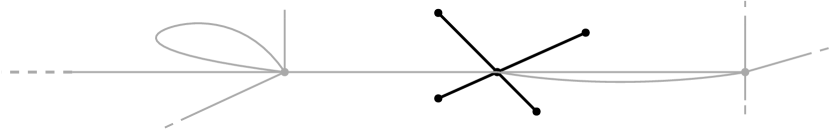
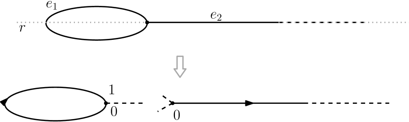
2. Infinite tadpole graph
Let be an infinite tadpole graph composed by two edges and . The self-closing edge , the “head”, is connected to in the vertex and it is parametrized in the clockwise direction with a coordinate going from to (the length of ). The “tail” is a half-line equipped with a coordinate starting from in and going to .
We consider as domain of functions , such that with . Let be the Hilbert space equipped with the norm induced by the scalar product
For , we introduce the spaces and the bilinear Schrödinger equation in
| (BSE*) |
The Laplacian is equipped with self-adjoint boundary conditions as is equipped with Neumann-Kirchhoff boundary conditions, i.e.
for every . We assume with and . We call the unitary propagator generated by the operator
The (BSE*) corresponds to the following Cauchy systems respectively in and with and
Let be an orthonormal system of made by eigenfunctions of and corresponding to the eigenvalues such that
We define and, for , the spaces
| (2) |
equipped with the norms
2.1. Well-posedness
Proposition 2.1.
Let and . There exists a unique mild solution of the (BSE*) in , i.e. a function such that
| (3) |
Moreover, there exists so that , while for every and
Proof.
The statement is proved by using the techniques developed in the proof of [Duc18b, Proposition 4.1], which generalize the ones of [BL10, Lemma 1; Proposition 2].
1) Let . We notice for almost every and . Let so that
We prove . For such that ,
Now, there exists so that
We notice for almost every and . Thus,
From [Duc18b, Proposition B.6], there exist uniformly bounded for in bounded intervals such that
and . For every , the last inequality shows that and the provided upper bound is uniform. The Dominated Convergence Theorem leads to .
2) As , we have thanks to the arguments of [Duc20, Remark 2.1]. Let . We consider the map with
For every , from the first point of the proof, there exists uniformly bounded for lying on bounded intervals, such that
If is small enough, then is a contraction and Banach Fixed Point Theorem implies that there exists such that When is not sufficiently small, one considers a partition of with . We choose a partition such that each is so small that the map , defined on the interval , is a contraction and we apply the Banach Fixed Point Theorem.
In conclusion, if , then . By multiplying (BSE*) with , we obtain that , which leads to for every and . The generalization for follows from a classical density argument. ∎
2.2. Global exact controllability
We recall that and respectively are an orthonormal system of made by eigenfunctions of and the corresponding eigenvalues. They are such that
Let be the unitary propagator representing the dynamics of (BSE*) at time for and with control .
Theorem 2.2.
Proof.
1) Local exact controllability in . For , let
We prove the existence of so that, for every , there exists such that To this purpose, we consider the map , the sequence with elements for , such that
with defined in (5). The local exact controllability of the bilinear Schrödinger equation in with is equivalent to the surjectivity of the map . As
the controllability is equivalent to the local surjectivity of . To this end, we use the Generalized Inverse Function Theorem ([Lue69, Theorem 1; p. 240]) and we study the surjectivity of the Fréchet derivative of with . Let with . As in the proof of [Duc19, Proposition 2.1], the map is the sequence of elements with so that
The surjectivity of corresponds to the solvability of the moments problem
| (4) |
By direct computation, we know and, for , there holds
Thus, there exists such that for every Now,
In conclusion, the solvability of is guaranteed by [Duc18b, Proposition B.5] since
2) Global exact controllability. Let be so that 1) is valid. Thanks to Remark B.3 (Appendix B), for any such that , there exist , and such that
and From 1), there exist such that
In conclusion, there exist and such that
3) Energetic controllability. The energetic controllability follows as for every and ∎
3. Generic graphs
Let be a generic infinite graph composed by edges of lengths and vertices .
Let the bilinear Schrödinger equation in the Hilbert space
| (BSE) |
The Laplacian is equipped with self-adjoint boundary conditions, is a bounded symmetric operator and . When the (BSE) is well-posed, we call the unitary propagator generated by We call and the external and the internal vertices of , i.e.
For every vertex of , we denote and each is considered to be parametrized with a coordinate going from to . We equip with the scalar product
We call the norm in and, for , we introduce the spaces
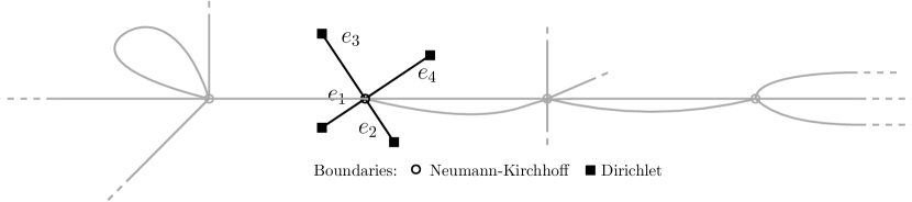
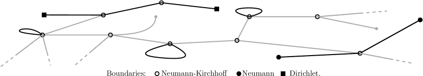
In the (BSE), the operator is a self-adjoint Laplacian such that the functions in satisfy the following boundary conditions. Each is equipped with Neumann-Kirchhoff boundary conditions when the function is continuous in and
The derivatives are assumed to be taken in the directions away from the vertex (outgoing directions). In addition, the external vertices are equipped with Dirichlet or Neumann type boundary conditions. As in [Duc18b], we respectively call (), () and () the Neumann-Kirchhoff, Dirichlet and Neumann boundary conditions characterizing .
In the current work, we denote a graph as quantum graph when a self-adjoint Laplacian is defined on . We say that is equipped with one of the previous boundaries in a vertex , when each satisfies it in . By simplifying the notation of [Duc18b], we say that is equipped with () (or ()) when, for every , the function satisfies () (or ()) in every and verifies () in every . In addition, the graph is equipped with (/) when, for every and , the function satisfies () or () in and verifies () in every .
Let be an orthonormal system of made by eigenfunctions of and let be the corresponding eigenvalues. We define
with . Let () be the external (internal) vertices of .
Remark 3.1.
Let be such that (the spectrum of in the Hilbert space ). As is a compact graph, thanks to [Duc18b, Lemma 2.3], for every we have in , i.e. there exists such that
Now, is the quantum graph associated to a Laplacian so that
Let be the entire part of . For , we define the spaces
| (5) |
We equip the space for with the norm such that
Let and
Assumptions I ().
The operator is bounded and symmetric in , .
-
(1)
There exists such that for every .
-
(2)
For every such that and it holds
Assumptions II ().
Let one of the following points be satisfied.
-
(1)
When is equipped with (/) and , there exists such that
-
(2)
When is equipped with () and , there exist and such that and
-
(3)
When is equipped with () and , there exists such that If , then there exists such that there holds
From now on, we omit the terms and from the notations of Assumptions I and Assumptions II when their are not relevant.
3.1. Interpolation properties and well-posedness
We present interpolation properties for the spaces with . The result follows from [Duc18b, Proposition 4.2] as is a compact graph.
Proposition 3.2 (Proposition 4.2; [Duc18b]).
Let be an orthonormal system of made by eigenfunctions of .
1) If the quantum graph is equipped with (/), then
2) If the quantum graph is equipped with (), then
3) If the quantum graph is equipped with (), then
In the following section, we ensure the well-posedness of the (BSE).
Proposition 3.3.
Let the couple satisfy Assumptions II with and . Let be introduced in Assumptions II.
1) Let and . Let The map and there exists uniformly bounded for lying on intervals so that
2) Let and . There exists a unique mild solution of the (BSE) (relation ). Moreover, there exists so that, for every and ,
Proof.
The result is obtained by generalizing the proof of Proposition 2.1.
1) (a) Assumptions II.1 . Let for almost every , and . We prove that . First, and
| (6) |
We estimate for each and . We suppose . Let be the derivative of and be the primitive of so that We call the two points of the boundaries of an edge . For every , and , there exist so that
| (7) |
We consider [Duc18b, Lemma 2.3] since is a compact graph. There exist such that for every and
| (8) |
Remark 3.4.
We notice for every where is a self-adjoint Laplacian with compact resolvent. Thus,
and, for almost every and ,
Let for be so that and Now,
for every and . Thus, and there exists such that, for every and , we have . Thanks to the identities , and to Remark 3.4, there exists such that
| (9) |
Again, as is a compact graph, [Duc18b, Lemma 2.4] is valid for the sequence and, from [Duc18b, Proposition B.6], there exist uniformly bounded for in bounded intervals such that
| (10) |
and . We underline that the identity is also valid when , which is proved by isolating the term with and by repeating the steps above. For every , the inequality (10) shows that . The provided upper bounds are uniform and the Dominated Convergence Theorem leads to .
Let for almost every and . The same techniques adopted above shows that .
We denote for and . Let be the space of functions so that belongs to a Banach space for almost every and . The first part of the proof implies
Classical interpolation results (as [BL76, Theorem 4.4.1] with ) lead to with . Thanks to Proposition 3.2, if and for almost every and , then , which achieves the proof.
(b) Assumptions II.3 . If is equipped with (), then and from Proposition 3.2. As above, if for almost every and , then , while if for almost every and , then . From the interpolation techniques, if and for almost every and , then .
(c) Assumptions II.2 . Let for almost every and and be equipped with . In this framework, the last line of is zero. Indeed, as and, for , we have thanks to the () boundary conditions (the terms assume different signs according to the orientation of the edges connected in ). After, for every , thanks to the in , we have . From , we obtain
Now, is a Hilbert basis of and we proceed as in (8), (9) and (10). From [Duc18b, Proposition B.6], there exists uniformly bounded such that
If for almost every and , then Equivalently when for almost every and , we have As above, from Proposition 3.2, if and for almost every and , then
3.2. Controllability results
Definition 3.5.
Let be an orthonormal system of made by eigenfunctions of and let be the corresponding eigenvalues.
Before proceeding with the main result of the work, we notice the following fact. As is a compact graph, [Duc18b, Lemma 2.4] implies
| (11) |
(the parameter is equal to when corresponds to an interval).
Theorem 3.6.
Let be a quantum graph. We assume that
| (12) |
If satisfies Assumptions I and Assumptions II for , then the (BSE) is globally exactly controllable in for with from Assumptions I and energetically controllable in
Proof.
1) Local exact controllability. The proof follows as the point 1. of the proof of Theorem 2.2 by considering instead of . The peculiarity of this case is that assumes value in while in
In the current framework, the moments problem is defined for sequences in and thanks to the point 1. of Assumptions I. The solvability of is guaranteed by [Duc18b, Proposition B.5] thanks to since
4. Example
Let a star graph be a graph composed by edges . Each edge is
parametrized with a coordinate going from to the length of the edge . We set the in the external vertex belonging to .

Let be a graph containing as sub-graph a star graph equipped with () and composed by the edges . Let the couple of edges be of length , while be long .
Corollary 4.1.
Let be such that for every and
while for every . There exists an orthonormal system composed by eigenfunctions of such that the (BSE) is globally exactly controllable in with and energetically controllable in
Proof.
Let be some eigenfunctions of and the corresponding eigenvalues. We define and so that, for every , there exist and so that for and
Spectral behaviour. We notice that are irrationally independent and is an algebraic irrational number. As in the proof of [Duc18b, Lemma 2.6], thanks [Duc18b, Proposition A.1], for every there exist and such that
Assumptions I.1 For the entire part of , we have
The last relation implies the existence of such that for every and the point 1. of Assumptions I() is verified.
Assumptions I.2 We prove that the point 2. of Assumptions I() is satisfied. By direct computation, it follows
For so that and , we have
Indeed, the identity is never verified as it would imply
Remark 4.2.
We notice that, for every different numbers, such that , it holds . Indeed, we have
Now, if , then and since , which is impossible as .
In conclusion, implies and then
Thus, and Assumptions I() is valid.
Remark 4.3.
As in [Duc18a, Section 6], the techniques just developed are valid when contains suitable sub-graphs denoted “uniform chains”. A uniform chain is a sequence of edges of equal length connecting vertices such that . We also assume that either are equipped with (), , or and are equipped with ().
Let contain uniform chains , composed by edges of lengths . Let and be respectively the sets of indices such that the external vertices of are equipped with and , while . If , then the energetic controllability can be guaranteed in
Acknowledgments. The second author has been financially supported by the ISDEEC project by ANR-16-CE40-0013.
Appendix A Analytic perturbation
We adapt the perturbation theory from [Duc20, Appendix B] as done in [Duc18b, Appendix C]. Indeed, [Duc20] considers the (BSE) on and is the Dirichlet Laplacian. As in [Duc20, Appendix B], we decompose
We consider as a perturbative term of . Let us consider the (BSE) with a quantum graph. Let be an orthonormal system of made by eigenfunctions of and let be the relative eigenvalues. Let be an orthonormal system in made by eigenfunctions of and be the relative eigenvalues.
Remark.
From (11), we notice that there does not exist consecutive such that This fact leads to a partition of in subsets that we call with . By definition, for every , if , then while if and , then This also defines an equivalence relation in such that are equivalent if and only if there exists such that The sets are the corresponding equivalence classes and .
We denote as the application mapping in such that , while is such that . Moreover, is so that . Let and be the projector onto We define the orthogonal projector.
Lemma A.1.
Let the hypotheses of Theorem 3.6 be satisfied. There exists a neighborhood of in such that there exists so that
Moreover, for , the operator is invertible with bounded inverse from to for every .
Proof.
The claim follows as [Duc20, Lemma B.2 & Lemma B.3].∎
Lemma A.2.
Let the hypotheses of Theorem 3.6 be satisfied. There exists a neighborhood of in such that, up to a countable subset and for every ,
Proof.
For , we decompose where , and is orthogonal to for every . Moreover, and for every and
Now, Lemma A.1 leads to the existence of such that, for every ,
| (13) |
and Let for every . We compute and
Thanks to , it follows . Let
As , it follows uniformly in . Thanks to
we have uniformly in . Now, there exists such that
| (14) |
where uniformly in . When , the identity is still valid. For each such that , there exists such that uniformly in and
Thanks to the third point of Assumptions I, there exists a neighborhood of in small enough such that, for each , we have that every function is not constant and analytic. Now, is a discrete subset of and
is a countable subset of , which achieves the proof of the first claim. The second relation is proved with the same technique. For , the analytic function is not constantly zero since and is a countable subset of . ∎
Lemma A.3.
Let the hypotheses of Theorem 3.6 be satisfied. Let and for introduced in Assumptions II. Let such that (the spectrum of in the Hilbert space ) and such that is a positive operator. There exists a neighborhood of in such that,
| (15) |
Proof.
Let be the neighborhood provided by Lemma A.2. The proof follows the one of [Duc20, Lemma B.6]. We suppose that and is positive such that we can assume . If , then the proof follows from the same arguments.
Thanks to Remark 3.1, we have in . We prove the existence of such that, for every ,
| (16) |
Let . The relation is proved by iterative argument. First, it is true for when as there exists such that for . When if and for , then there exist such that, for ,
and . Second, we assume be valid for when for and for every . We prove for when for and for every . Now, there exists such that for every . Thus, as , there exist such that, for every ,
As in the proof of [Duc20, Lemma B.6], the relation (16) is valid for any when for and for and for every . The opposite inequality follows by decomposing
In our framework, Assumptions II ensure that the parameter is equal to .
If the second point of Assumptions II is verified for , then preserves and for introduced in Assumptions II. Proposition 3.2 claims that and the argument of [Duc20, Remark 2.1] implies (also as ). Thus, the identity (15) is valid because , and with . If the third point of Assumptions II is verified for , then , and for . The claim follows thanks to Proposition 3.2 since stabilizes and for introduced in Assumptions II. If instead, then the conditions and are sufficient to guarantee (15).∎
Appendix B Global approximate controllability
Let us consider the notation introduced in Section 3.
Definition B.1.
The (BSE) is said to be globally approximately controllable in with when, for every , such that and , there exist and such that .
Proposition B.2.
Let satisfy Assumptions I and Assumptions II for and . The (BSE) is globally approximately controllable in for with from Assumptions II .
Proof.
In the point 1) of the proof, we suppose that admits a non-degenerate chain of connectedness (see [BdCC13, Definition 3]). We treat the general case in the point 2) .
1) (a) Preliminaries. Let be the orthogonal projector for every Up to reordering of , the couples for admit non-degenerate chains of connectedness in . Let and for
-
Claim.
(17)
Let and . We define such that is an orthonormal basis of . The operator is the unitary map such that for every The provided definition implies . Thus, for every , there exists large enough satisfying the claim.
1) (b) Finite dimensional controllability. Let be the set of such that and with implies for . For every and , we define the matrix with elements , and for Let and . Fixed a piecewise constant control taking value in and , we introduce the control system on
| (18) |
-
Claim. is controllable, i.e. for , there exist , , such that
For every , we define the matrices , and as follow. For we have and while and Moreover, for and We consider the basis of
Thanks to [Sac00, Theorem 6.1], the controllability of (18) is equivalent to prove that for the Lie algebra of The claim si valid as it is possible to obtain the matrices , and for every by iterated Lie brackets of elements in .
1) (c) Finite dimensional estimates. Let and be defined in 1) (a). Thanks to the previous claim and to the fact that , there exist , and such that
| (19) |
-
Claim. For every and from , there exist and such that for every and
(20) (21)
We consider the results developed in [Cha12, Section 3.1 & Section 3.2] by Chambrion and leading to [Cha12, Proposition 6] since admits a non-degenerate chain of connectedness ([BdCC13, Definition 3]). Each is a rotation in a two dimensional space for every and this work allows to explicit and satisfying such that for every and
| (22) |
As , we have for
1) (d) Infinite dimensional estimates.
-
Claim. Let . There exist such that for every , there exist and such that and
(23)
Let 1) (c) be valid with . Although, the following result is valid for any . There exists such that . Thanks to , there exists large enough such that,
The identity leads to the existence of such that for every , there exist and such that and
| (24) |
The relation and the triangular inequality achieve the claim.
1) (e) Global approximate controllability with respect to the -norm. Let and .
-
Claim. There exist such that for every , there exist and such that and
(25)
We assume that , but the same proof is also valid for the generic case. From the point 1) (d), there exist two controls respectively steering close to and close to . Vice versa, thanks to the time reversibility, there exists a control steering close to . In other words, there exist , and such that
The chosen controls and satisfy (25). The claim is proved as
1) (f) Global approximate controllability in higher regularity norm. Let with and . Let be such that and .
-
Claim. There exist and such that .
We consider the propagation of regularity developed by Kato in [Kat53]. We notice that is maximal dissipative in for suitable . Let and . We know that and the arguments of [Duc20, Remark 2.1] imply that . For and , we have
We know for and . Equivalently,
We call and the propagator generated by such that . Thanks to [Kat53, Section 3.10], for every , it follows
For every , and , there exists depending on such that
| (26) |
Now, we notice that, for every , from the Cauchy-Schwarz inequality, we have and there exists such that . By following the same idea, for every , there exist and such that
| (27) |
In conclusion, the point 1) (e), the relation and the relation ensure the claim.
1) (g) Conclusion. Let be defined in Assumptions II. If , then and the global approximate controllability is verified in since If , then with from Assumptions II. Now, , thanks to Proposition 3.2, and implies . The global approximate controllability is verified in since If , then for and from Proposition 3.2. Now, that implies . The global approximate controllability is verified in since
2) Generalization. Let do not admit a non-degenerate chain of connectedness and
If satisfies Assumptions I and Assumptions II, then Lemma A.2 and Lemma A.3 (Appendix A) are valid. We consider belonging to the neighborhoods provided by the two lemmas and we denote a Hilbert basis of made by eigenfunctions of . The steps of the point 1) can be repeated by considering the sequence instead of and the spaces in substitution of with . The claim is equivalently proved thanks to Lemma A.3. ∎
Remark B.3.
As Proposition B.2, the (BSE*) is globally approximately controllable in (defined in ). In other words, for every , such that and , we have
Indeed, for every so that and such that
there exists so that, thanks to Remark we have
In conclusion, the statement of Lemma A.2 is valid when is small enough. Thus, admits a non-degenerate chain of connectedness. The arguments adopted in the proof of Proposition B.2 lead to the claim.
References
- [AAN17] F. Ali Mehmeti, K. Ammari and S. Nicaise, Dispersive effects for the Schrödinger equation on a tadpole graph, Journal of Mathematical Analysis and Applications, 448 (2017), 262–280
- [AAN15] F. Ali Mehmeti, K. Ammari and S. Nicaise, Dispersive effects and high frequency behaviour for the Schrödinger equation in star-shaped networks, Port. Math., 72 (2015), 309–355.
- [Alt02] C. Altafini, Controllability of quantum mechanical systems by root space decomposition, J. Math. Phys., 43 (2002), 2051–2062.
- [BCMS12] U. Boscain, F. Chittaro, P. Mason and M. Sigalotti, Adiabatic control of the Schrödinger equation via conical intersections of the eigenvalues, IEEE Trans. Automat. Control., 57 (2012), 1970–1983.
- [BCS14] U. Boscain, M. Caponigro, and M. Sigalotti, Multi-input Schrödinger equation: controllability, tracking, and application to the quantum angular momentum, J. Differential Equations, 256 (2014), 3524–3551.
- [BdCC13] N. Boussaïd, M. Caponigro and T. Chambrion. Weakly coupled systems in quantum control, IEEE Trans. Automat. Control., 58 (2013), 2205–2216.
- [BGRS15] U. Boscain, J.-P. Gauthier, F. Rossi and M. Sigalotti, Approximate controllability, exact controllability, and conical eigenvalue intersections for quantum mechanical systems, Comm. Math. Phys., 333 (2015), 1225–1239.
- [BL76] J. Bergh and J. Löfström, Interpolation spaces. An introduction, Grundlehren der Mathematischen Wissenschaften, No. 223, Springer-Verlag, Berlin-New York, 1976.
- [BL10] K. Beauchard and C. Laurent, Local controllability of 1D linear and nonlinear Schrödinger equations with bilinear control, J. Math. Pures Appl., 94 (2010), 520–554.
- [BLR92] C. Bardos, G. Lebeau and J. Rauch, Sharp sufficient conditions for the observation, control, and stabilization of waves from the boundary, SIAM J. Control Optim., 30 (1992), 1024–1065.
- [BMS82] J.-M. Ball, J.-E. Marsden, and M. Slemrod, Controllability for distributed bilinear systems, SIAM J. Control Optim., 20 (1982), 575–597.
- [Cha12] T. Chambrion, Periodic excitations of bilinear quantum systems, Automatica J. IFAC., 48 (2012), 2040–2046.
- [Cor07] J.-M. Coron, Control and nonlinearity, volume 136, Mathematical Surveys and Monographs, American Mathematical Society, Providence, RI, 2007.
- [Duc18a] A. Duca, Global exact controllability of bilinear quantum systems on compact graphs and energetic controllability, submitted: https://arxiv.org/abs/1809.06249, 2018.
- [Duc18b] A. Duca, Bilinear quantum systems on compact graphs: well-posedness and global exact controllability, submitted: https://hal.archives-ouvertes.fr/hal-01830297, 2018.
- [Duc19] A. Duca. Controllability of bilinear quantum systems in explicit times via explicit control fields. To be published in International Journal of Control, 2019.
- [Duc20] A. Duca. Simultaneous global exact controllability in projection of infinite 1D bilinear Schrödinger equations. Dynamics of Partial Differential Equations, 17(3):275–306, 2020.
- [Kat53] T. Kato, Integration of the equation of evolution in a Banach space. J. Math. Soc. Japan., 5 (1953), 208–234.
- [Kuc04] P. Kuchment, Quantum graphs. I, Some basic structures, Special section on quantum graphs, Waves Random Media, 14 (2004), S107–S128.
- [Lio83] J.-L. Lions, Contrôle des systèmes distribués singuliers, volume 13, Méthodes Mathématiques de l’Informatique, Gauthier-Villars, Montrouge, 1983.
- [Lue69] D.-G. Luenberger, Optimization by vector space methods, John Wiley & Sons, Inc., New York-London-Sydney, 1969.
- [Mir09] M. Mirrahimi, Lyapunov control of a quantum particle in a decaying potential, Ann. Inst. H. Poincaré Anal. Non Linéaire., 26 (2009), 1743–1765.
- [MN15] M. Morancey and V. Nersesyan, Simultaneous global exact controllability of an arbitrary number of 1D bilinear Schrödinger equations, J. Math. Pures Appl.,, 103 (2015), 228–254.
- [MOR08] A. Mercado, A. Osses and L. Rosier, Inverse problems for the Schrödinger equation via Carleman inequalities with degenerate weights, Inverse Problems, 24 (2008), 015017, 18.
- [Mor14] M. Morancey, Simultaneous local exact controllability of 1D bilinear Schrödinger equations, Ann. Inst. H. Poincaré Anal. Non Linéaire., 31 (2014), 501–529.
- [Ner10] V. Nersesyan, Global approximate controllability for Schrödinger equation in higher Sobolev norms and applications, Ann. Inst. H. Poincaré Anal. Non Linéaire, 27 (2010), 901–915.
- [Sac00] Yu.-L. Sachkov, Controllability of invariant systems on Lie groups and homogeneous spaces. Dynamical systems, 8. J. Math. Sci. (New York), 100 (2000), 2355–2427.