Abstract

A lattice system of spinor atoms or molecules experiencing quadratic Zeeman effect is considered. This can be an optical lattice with sufficiently deep wells at lattice sites, so that the system is in an isolating state, where atoms are well localized. But their effective spins can move in the presence of external magnetic fields. The dynamics of spins, starting from an initial nonequilibrium state, is investigated. The system is immersed into a magnetic coil of an electric circuit, creating a magnetic feedback field. Two types of quadratic Zeeman effect are treated, a nonresonant, so-called static-current quadratic Zeeman effect and a quasi-resonant alternating-current quadratic Zeeman effect. Spin dynamics in these conditions is highly nonlinear. Different regimes of spin dynamics, starting from a strongly nonequilibrium state, are studied. Conditions for realizing fast spin reversal are found, which can be used in quantum information processing and spintronics.

1 Introduction

Atomic (or molecular) systems interacting through dipolar and spinor forces have been a topic of intensive research in recent years, as can be inferred from the books and review articles [1, 2, 3, 4, 5, 6, 7, 8, 9]. A great advantage of these systems is the richness of their properties and the possibility of tuning the latter in a rather wide range.

In the present paper, we study spinor atomic systems forming lattices. These can be either self-organized lattices or optical lattices created by laser beams. Our main concern is not the motion of atoms, but the dynamics of effective spin variables. Therefore we consider deep lattices, where atoms, being well localized, form insulating states. Thus the atomic motion is frozen, while effective spins can move, especially if external magnetic fields are applied.

In the presence of external magnetic fields, spinor atoms can experience quadratic Zeeman effect. There are, actually, two types of the effect. One is the nonresonant static-current quadratic Zeeman effect arising in atoms possessing hyperfine structure, hence a nonzero nuclear spin [10, 11, 12, 13].

The other type of quadratic Zeeman effect is the so-called quasi-resonant alternating-current quadratic Zeeman effect, due to the alternating-current Stark shift. The latter can be produced by applying either a linearly polarized microwave driving field inducing hyperfine transitions in an atom [14, 15, 16] or applying off-resonance linearly polarized light inducing transitions between internal spin states [17, 18, 19, 20]. The linearly polarized quasiresonance alternating fields exert the quadratic shift along the polarization axis.

We shall take into account both these phenomena, the static-current quadratic Zeeman effect and the alternating-current quadratic Zeeman effect. Our aim is to study how the presence of these effects influences spin dynamics in spinor lattices and how this influence could be employed for governing spin motion.

The main difference of the present work from the previous publications on spinor atomic systems is in the following five points:

1. We concentrate our attention on the study of spin dynamics, while the spatial motion of atoms is frozen in a deep insulating lattice. This regime is important for spintronics.

2. We consider strongly nonequilibrium dynamics, but not slight deviations from equilibrium, which requires to deal with special methods of solving spin evolution equations.

3. Both types of the quadratic Zeeman effect are taken into account, the nonresonant static-current, as well as the quasi-resonant alternating-current effects, which provides efficient tools for influencing spin motion.

4. In addition to a stationary magnetic field, the sample is subject to the action of a feedback magnetic field formed by a magnetic coil of an electric circuit. Such a configuration allows for a powerful possibility of regulating spin dynamics.

5. Conditions for realizing fast spin reversal are investigated. This mechanism can be employed in spintronics and information processing.

2 Hamiltonian of spinor atoms

A spinor atom (or molecule) is characterized by a total angular momentum ${\bf F}$ that is a matrix vector

$${\bf F}=[{\bf F}_{mn}]=\sum_{\alpha}F^{\alpha}{\bf e}_{\alpha}=\sum_{\alpha}[F^{\alpha}_{mn}]{\bf e}_{\alpha}\qquad(\alpha=x,y,z)\;,$$ (1)

with the matrix elements labeled by the index $m=-F,-F+1,\ldots,F$. The related field operators are the columns

$$\hat{\psi}({\bf r})=[\hat{\psi}_{m}({\bf r})]\qquad(m=-F,-F+1,\ldots,F)\;.$$ (2)

The time dependence of the field operators is assumed, but not shown for brevity. The total Hamiltonian of a system of spinor atoms can be written as a sum of three terms

$$\hat{H}=\hat{H}_{0}+\hat{H}_{Z}+\hat{H}_{int}\;.$$ (3)

Here the first term is the single-atom part not containing the angular momentum,

$$\hat{H}_{0}=\int\hat{\psi}^{\dagger}({\bf r})\left[-\hbar^{2}\;\frac{\nabla^{2}}{2m}+U({\bf r})\right]\hat{\psi}({\bf r})\;d{\bf r}\;,$$ (4)

where $U({\bf r})$ is an external field, for instance, due to an optical lattice.

The second term is the Zeeman energy Hamiltonian

$$\hat{H}_{Z}=\hat{H}_{LZ}+\hat{H}_{QZ}$$ (5)

including the parts caused by the linear and quadratic Zeeman effects. The linear Zeeman term is

$$\hat{H}_{LZ}=-\mu_{F}\int\hat{\psi}^{\dagger}({\bf r})\;{\bf B}\cdot{\bf F}\;\hat{\psi}({\bf r})\;d{\bf r}\;,$$ (6)

where $\mu_{F}=-g_{F}\mu_{B}$, with $g_{F}$ being the Landé factor and $\mu_{B}$, Bohr magneton. The external magnetic field ${\bf B}={\bf B}({\bf r},t)$, in general, is a function of spatial and time variables.

As is mentioned in the Introduction, quadratic Zeeman effect can be of two types, nonresonant static-current Zeeman effect and quasi-resonant alternating-current Zeeman effect. The corresponding Hamiltonian is

$$\hat{H}_{QZ}=Q_{Z}\int\hat{\psi}^{\dagger}({\bf r})\;({\bf B}\cdot{\bf F})^{2}\;\hat{\psi}({\bf r})\;d{\bf r}\;+\;q_{Z}\int\hat{\psi}^{\dagger}({\bf r})\;(F^{z})^{2}\;\hat{\psi}({\bf r})\;d{\bf r}\;,$$ (7)

with the static-current Zeeman parameter

$$Q_{Z}=\mp\;\frac{\mu_{F}^{2}}{\Delta W(1+2I)^{2}}\;,$$ (8)

in which $\Delta W$ is a hyperfine energy splitting and $I$ is nuclear spin, and with the alternating-current Zeeman parameter

$$q_{Z}=-\;\frac{\hbar\Omega^{2}_{R}}{4\Delta}\;,$$ (9)

where $\Omega_{R}$ is the Rabi frequency of the driving alternating field and $\Delta$ is the detuning from an internal (spin or hyperfine) transition. The polarization of the driving field is assumed to be along the axis $z$. The sign minus or plus in the static-current Zeeman parameter $Q_{Z}$ is defined by the relative alignment of the nuclear and the total electron spin projections of the atom: minus for parallel projections, while plus for antiparallel projections. The sign of the alternating-current Zeeman parameter $q_{Z}$ can be varied by using either positive or negative detuning. The parameter $q_{Z}$ can be tailored at high resolution and rapidly adjusted to the desired values.

The interaction Hamiltonian

$$\hat{H}_{int}=\hat{H}_{F}+\hat{H}_{D}$$ (10)

is the sum of a term $\hat{H}_{F}$ describing local interactions of atoms, each having an angular momentum ${\bf F}$, and of a term $\hat{H}_{D}$ corresponding to nonlocal dipolar interactions. For rotationally symmetric pair collisions in the $s$-wave approximation, the angular momentum $f$ of the pair of colliding atoms has to be even, which is valid for bosons as well as for fermions. Then the binary collisions of atoms are characterized by the interaction potential

$$\Phi_{F}({\bf r})=\delta({\bf r})\sum_{f}4\pi\hbar^{2}\;\frac{a_{f}}{m}\hat{P}_{f}\;,$$ (11)

where $a_{f}$ is the scattering length of a pair of atoms with the angular momentum of the pair $f$ and $\hat{P}_{f}$ is a projection operator onto a state with an even angular momentum $f$. The Hamiltonian of such local atomic interactions reads as

$$\hat{H}_{F}=\frac{1}{2}\sum_{klmn}\int\hat{\psi}^{\dagger}_{k}({\bf r})\hat{\psi}^{\dagger}_{l}({\bf r})\Phi_{klmn}\hat{\psi}_{m}({\bf r})\hat{\psi}_{n}({\bf r})\;d{\bf r}\;,$$ (12)

with $\Phi_{klmn}$ being a matrix element of potential (11).

Atoms, possessing angular momenta, also interact through dipolar forces. The related dipolar interaction Hamiltonian is

$$\hat{H}_{D}=\frac{\mu_{F}}{2}\sum_{klmn}\int\hat{\psi}^{\dagger}_{k}({\bf r})\hat{\psi}^{\dagger}_{l}({\bf r}^{\prime})\hat{\psi}_{m}({\bf r}^{\prime})\hat{\psi}_{n}({\bf r})D_{klmn}({\bf r}-{\bf r}^{\prime})\;d{\bf r}\;d{\bf r}^{\prime}\;,$$ (13)

with the dipolar interaction potential

$$D_{klmn}({\bf r})=\frac{({\bf F}_{kn}\cdot{\bf F}_{lm})-3({\bf F}_{kn}\cdot{\bf n})(({\bf F}_{lm}\cdot{\bf n})}{r^{3}}\;,$$ (14)

where $r\equiv|{\bf r}|$ and ${\bf n}\equiv{\bf r}/r$. Strictly speaking, the dipolar interactions should be regularized by taking into account the sizes of atoms and, in general, screening effects [8, 9, 21]. The regularized dipolar potential can be written in the form

$$\overline{D}_{klmn}({\bf r})=\Theta(r-b_{F})D_{klmn}({\bf r})\exp(-\varkappa_{F}r)\;,$$ (15)

in which $\Theta(r)$ is a unit-step function, $b_{F}$ is a short-range cutoff, and $\varkappa_{F}$ is a screening parameter. The regularized potential automatically excludes unphysical self-action, so that Hamiltonian (13) can be represented as

$$\hat{H}_{D}=\frac{\mu_{F}}{2}\sum_{klmn}\int\hat{\psi}^{\dagger}_{k}({\bf r})\hat{\psi}^{\dagger}_{n}({\bf r})\overline{D}_{klmn}({\bf r}-{\bf r}^{\prime})\hat{\psi}_{l}({\bf r}^{\prime})\hat{\psi}_{m}({\bf r}^{\prime})\;d{\bf r}\;d{\bf r}^{\prime}\;.$$ (16)

In what follows, we shall denote, for short, the dipolar potential as $D_{klmn}({\bf r})$, while keeping in mind its regularized form, when it is necessary to avoid unphysical consequences.

3 Deep insulating lattice

Suppose the atoms form a lattice, with the lattice vectors ${\bf a}_{j}$, where the index $j=1,2,\ldots,N$ enumerates lattice sites. Resorting to the single-band approximation, the field operators can be expanded over Wannier functions,

$$\hat{\psi}_{m}({\bf r})=\sum_{j}\hat{c}_{jm}w({\bf r}-{\bf a}_{j})\;.$$ (17)

The Wannier functions are assumed to be independent of the hyperfine index and can be chosen to be well localized [22], so that the lattice is insulating and intersite tunneling can be neglected.

It is possible to introduce effective spin operators

$${\bf S}_{j}\equiv\sum_{mn}\hat{c}^{\dagger}_{jm}{\bf F}_{mn}\hat{c}_{jn}$$ (18)

that are localized in the lattice sites. These operators satisfy the standard spin algebra for any type of statistics of atoms, whether bosons or fermions.

For a deep lattice, without tunneling, the total Hamiltonian (3) can be written as the sum

$$\hat{H}=\hat{H}_{L}+\hat{H}_{S}$$ (19)

of the local Hamiltonian

$$\hat{H}_{L}=\hat{H}_{0}+\hat{H}_{F}$$ (20)

and of the effective spin Hamiltonian

$$\hat{H}_{S}=\hat{H}_{Z}+\hat{H}_{D}\;.$$ (21)

The local Hamiltonian (20) can be shown [9] to commute with the spin Hamiltonian $H_{S}$, which we illustrate below. Therefore spin dynamics is governed only by the effective spin Hamiltonian.

The local Hamiltonian depends on the hyperfine angular momentum of atoms. Thus for $F=1$, the components of the angular momentum are

$$F_{mn}^{x}=\frac{1}{\sqrt{2}}\;(\delta_{m\;n-1}+\delta_{m\;n+1})\;,\qquad F_{mn}^{y}=\frac{i}{\sqrt{2}}\;(\delta_{m\;n-1}-\delta_{m\;n+1})\;,$$

$$F_{mn}^{z}=m\delta_{mn}\qquad(m,n=-1,0,1)\;.$$

As a result, we have

$$\hat{H}_{L}=\sum_{j}\left[h_{j}\hat{n}_{j}+\frac{\overline{c}_{0}}{2}\;\hat{n}_{j}(\hat{n}_{j}+1)+\frac{\overline{c}_{2}}{2}\;\left({\bf S}_{j}^{2}-2\hat{n}_{j}\right)\right]\;,$$ (22)

with the local-site energy

$$h_{j}\equiv\int w^{*}({\bf r}-{\bf a}_{j})\left[-\hbar^{2}\;\frac{\nabla^{2}}{2m}+U({\bf r})\right]w({\bf r}-{\bf a}_{j})\;d{\bf r}\;,$$ (23)

the operator density of atoms

$$\hat{n}_{j}\equiv\sum_{m}\hat{c}^{\dagger}_{jm}\hat{c}_{jm}\;,$$ (24)

and the interaction parameters

$$\overline{c}_{0}\equiv c_{0}\int|w({\bf r}-{\bf a}_{j})|^{4}\;d{\bf r}\;,\qquad\overline{c}_{2}\equiv c_{2}\int|w({\bf r}-{\bf a}_{j})|^{4}\;d{\bf r}\;,$$ (25)

in which

$$c_{0}\equiv\frac{4\pi}{3m}\;\hbar^{2}(2a_{2}+a_{0})\;,\qquad c_{2}\equiv\frac{4\pi}{3m}\;\hbar^{2}(a_{2}-a_{0})\;.$$ (26)

Here $a_{0}$ and $a_{2}$ are the scattering lengths for the collisions of atoms with the moments of atom pairs $f=0$ and $f=2$, respectively.

If the external magnetic field varies in space slower than the variation of the well localized Wannier functions, then the Zeeman Hamiltonian (5) takes the form

$$\hat{H}_{Z}=\sum_{j}\left[-\mu_{F}{\bf B}_{j}\cdot{\bf S}_{j}+Q_{Z}({\bf B}_{j}\cdot{\bf S}_{j})^{2}+q_{Z}(S_{j}^{z})^{2}\right]\;,$$ (27)

where ${\bf B}_{j}\equiv{\bf B}({\bf a}_{j})$. The dipolar Hamiltonian (13), for well localized atoms, becomes

$$\hat{H}_{D}=\frac{1}{2}\sum_{i\neq j}\;\sum_{\alpha\beta}D_{ij}^{\alpha\beta}S_{i}^{\alpha}S_{j}^{\beta}\;,$$ (28)

with the dipolar tensor

$$D_{ij}^{\alpha\beta}=\frac{\mu_{F}^{2}}{r_{ij}}\;(\delta_{\alpha\beta}-3n_{ij}^{\alpha}n_{ij}^{\beta})\exp(-\varkappa_{F}r_{ij})\;,$$ (29)

in which

$$r_{ij}\equiv|{\bf r}_{ij}|\;,\qquad{\bf n}_{ij}\equiv\frac{{\bf r}_{ij}}{r_{ij}}\;,\qquad{\bf r}_{ij}\equiv{\bf r}_{i}-{\bf r}_{j}\;.$$

For generality, we keep here the screening factor, which, although, is not principal for the following. If the screening is absent, then one should set $\varkappa_{F}=0$. The short-range cutoff can be omitted here, since the summation in Eq. (28) does not include coinciding lattice indices. A detailed derivation of Hamiltonian (19) for atoms with $F=1$ in a deep lattice can be found in the review [9].

The external magnetic field consists of a constant field $B_{0}$ along the axis $z$ and of a feedback field $H$ along the axis $x$, so that

$${\bf B}_{j}=B_{0}{\bf e}_{z}+H{\bf e}_{x}\;.$$ (30)

For the following, it is convenient to use the ladder spin operators connected with the spin components

$$S_{j}^{x}=\frac{1}{2}\;(S_{j}^{+}+S_{j}^{-})\;,\qquad S_{j}^{y}=-\;\frac{i}{2}\;(S_{j}^{+}-S_{j}^{-})\;.$$

Then the Zeeman Hamiltonian reads as

$$\hat{H}_{Z}=\sum_{j}\left\{-\mu_{F}B_{0}S_{j}^{z}-\;\frac{\mu_{F}H}{2}\;(S_{j}^{+}+S_{j}^{-})+(Q_{Z}B_{0}^{2}+q_{Z})(S_{j}^{z})^{2}\;+\right.$$

$$+\;\frac{Q_{Z}H^{2}}{4}\;\left[(S_{j}^{+})^{2}+(S_{j}^{-})^{2}+S_{j}^{+}S_{j}^{-}+S_{j}^{-}S_{j}^{+}\right]\;+$$

$$\left.+\;\frac{Q_{Z}B_{0}H}{2}\;\left[(S_{j}^{+}+S_{j}^{-})S_{j}^{z}+S_{j}^{z}(S_{j}^{+}+S_{j}^{-})\right]\right\}\;.$$ (31)

And the dipolar term takes the form

$$\hat{H}_{D}=\frac{1}{2}\sum_{i\neq j}\left[a_{ij}\left(S_{i}^{z}S_{j}^{z}-\;\frac{1}{2}\;S_{i}^{+}S_{j}^{-}\right)+b_{ij}S_{i}^{+}S_{j}^{+}+b_{ij}^{*}S_{i}^{-}S_{j}^{-}+2c_{ij}S_{i}^{+}S_{j}^{z}+2c_{ij}^{*}S_{i}^{-}S_{j}^{z}\right]\;,$$ (32)

in which

$$a_{ij}\equiv D_{ij}^{zz}\;,\qquad b_{ij}\equiv\frac{1}{4}\;(D_{ij}^{xx}-D_{ij}^{yy}-2iD_{ij}^{xy})\;,\qquad c_{ij}\equiv\frac{1}{2}\;(D_{ij}^{xz}-iD_{ij}^{yz})\;.$$

Note that the short-range regularization, excluding self-action, implies that

$$D_{jj}^{\alpha\beta}=0\;,\qquad a_{jj}=b_{jj}=c_{jj}=0\;.$$

4 Spin equations of motion

The constant external magnetic field defines the Zeeman frequency

$$\omega_{0}\equiv-\mu_{F}B_{0}>0\;.$$ (33)

To simplify the following formulas, we introduce the effective quadratic Zeeman parameter

$$Q\equiv Q_{Z}B_{0}^{2}+q_{z}\;,$$ (34)

define the local spin fluctuating fields

$$\xi_{i}\equiv\frac{1}{\hbar}\sum_{j}(a_{ij}S_{j}^{z}+c_{ij}S_{j}^{+}+c_{ij}^{*}S_{j}^{-})\;,\qquad\varphi_{i}\equiv\frac{1}{\hbar}\sum_{j}\left(\frac{a_{ij}}{2}S_{j}^{-}-2b_{ij}S_{j}^{+}-2c_{ij}S_{j}^{z}\right)\;,$$ (35)

and use the notation

$$f_{j}\equiv-i\left(\frac{\mu_{F}H}{\hbar}+\varphi_{j}\right)\;.$$ (36)

Employing the Heisenberg equations of motion, we find the equation for the ladder spin operator

$$\frac{dS_{j}^{-}}{dt}=-i(\omega_{0}+\xi_{j})S_{j}^{-}+f_{j}S_{j}^{z}-\;\frac{i}{\hbar}\;Q(S_{j}^{-}S_{j}^{z}+S_{j}^{z}S_{j}^{-})\;+$$

$$+\;\frac{i}{2\hbar}\;Q_{Z}H^{2}\left[(S_{j}^{+}+S_{j}^{-})S_{j}^{z}+S_{j}^{z}(S_{j}^{+}+S_{j}^{-})\right]\;-$$

$$-\;\frac{i}{2\hbar}\;Q_{Z}B_{0}H\left[S_{j}^{+}S_{j}^{-}+S_{j}^{-}S_{j}^{+}-4(S_{j}^{z})^{2}+2(S_{j}^{-})^{2}\right]$$ (37)

and the equation for the longitudinal spin component

$$\frac{dS_{j}^{z}}{dt}=-\;\frac{1}{2}(f_{j}^{+}S_{j}^{-}+S_{j}^{+}f_{j})\;+$$

$$+\;\frac{i}{2\hbar}\;Q_{Z}H^{2}\left[(S_{j}^{-})^{2}-(S_{j}^{+})^{2}\right]+\frac{i}{2\hbar}\;Q_{Z}B_{0}H\left[(S_{j}^{-}-S_{j}^{+})S_{j}^{z}+S_{j}^{z}(S_{j}^{-}-S_{j}^{+})\right]\;.$$ (38)

From these equations, we can derive the equations for the statistical averages of spin components. We are looking for the equations for the following quantities: the average transverse spin variable

$$u=\frac{1}{SN}\sum_{j}\;\langle S_{j}^{-}\rangle\;,$$ (39)

the coherence intensity

$$w=\frac{1}{SN(N-1)}\sum_{i\neq j}\;\langle S_{i}^{+}S_{j}^{-}\rangle\;,$$ (40)

and the longitudinal spin polarization

$$s=\frac{1}{SN}\sum_{j}\;\langle S_{j}^{z}\rangle\;.$$ (41)

To get a complete set of equations, we need to decouple the spin correlation functions. For different lattice sites, we use the mean-field approximation

$$\langle S_{i}^{\alpha}S_{j}^{\beta}\rangle=\langle S_{i}^{\alpha}\rangle\langle S_{j}^{\beta}\rangle\qquad(i\neq j)\;.$$ (42)

But for binary spin forms at the same site this approximation cannot be used, since, for instance, when $S=1/2$, then there is the exact equality

$$S_{j}^{\alpha}S_{j}^{\beta}+S_{j}^{\beta}S_{j}^{\alpha}=0\qquad\left(S=\frac{1}{2}\right)\;,$$

while the standard mean-field approximation would result in a nonzero quantity. The correct approximation for such single-site binary combinations, for arbitrary spins, reads [23, 24, 25] as

$$\langle S_{j}^{\alpha}S_{j}^{\beta}+S_{j}^{\beta}S_{j}^{\alpha}\rangle=\left(2-\;\frac{1}{S}\right)\langle S_{j}^{\alpha}\rangle\langle S_{j}^{\beta}\rangle\;.$$ (43)

This decoupling is exact for $S=1/2$ and asymptotically exact for large spins.

The other difficulty is that, averaging the terms of the type $\sum_{j}\xi_{j}S^{\alpha}_{j}$, for an ideal lattice, in the mean-field approximation one gets zero, because of the property of the dipolar tensor

$$\sum_{j}D_{ij}^{\alpha\beta}=0\;,\qquad\sum_{j}a_{ij}=\sum_{j}b_{ij}=\sum_{j}c_{ij}=0\;.$$

A more refined method, retaining the input of local dipolar fluctuations, is based on stochastic quantization [26, 27]. For this purpose, we define the averages

$$\left\langle\frac{1}{N}\sum_{j}\xi_{j}S_{j}^{\alpha}\right\rangle=\xi_{S}\;\frac{1}{N}\sum_{j}\;\langle S_{j}^{\alpha}\rangle\;,\qquad\left\langle\frac{1}{N}\sum_{j}\varphi_{j}S_{j}^{\alpha}\right\rangle=\varphi_{S}\;\frac{1}{N}\sum_{j}\;\langle S_{j}^{\alpha}\rangle\;.$$ (44)

The variables $\xi_{S}$ and $\varphi_{S}$, describing local dipolar fluctuations, are treated as stochastic variables. It is straightforward to show that these variables are responsible for the existence of dipolar spin waves [28]. The random variables are modeled by a Gaussian white noise [29, 30, 31] defined by the stochastic averages

$$\langle\langle\xi_{S}(t)\rangle\rangle=\langle\langle\varphi_{S}(t)\rangle\rangle=0\;,\qquad\langle\langle\xi_{S}(t)\xi_{S}(t^{\prime})\rangle\rangle=2\gamma_{3}\delta(t-t^{\prime})\;,$$

$$\langle\langle\varphi^{*}_{S}(t)\varphi_{S}(t^{\prime})\rangle\rangle=2\gamma_{3}\delta(t-t^{\prime})\;,\qquad\langle\langle\xi_{S}(t)\varphi_{S}(t^{\prime})\rangle\rangle=\langle\langle\varphi_{S}(t)\varphi_{S}(t^{\prime})\rangle\rangle=0\;,$$ (45)

where $\gamma_{3}$ is the attenuation caused by dipolar spin fluctuations.

Averaging Eqs. (37) and (38) over spin variables, we take into account the existence of longitudinal, $\gamma_{1}$, and transverse, $\gamma_{2}$, attenuations [32, 33]. We define the frequency related to the quadratic Zeeman effect,

$$\omega_{Q}\equiv(2S-1)\;\frac{Q}{\hbar}$$ (46)

and the effective frequency of spin rotation

$$\omega_{s}\equiv\omega_{0}+\omega_{Q}s=\omega_{0}(1+As)\;,$$ (47)

with the dimensionless quadratic Zeeman effect parameter

$$A\equiv\frac{\omega_{Q}}{\omega_{0}}=(2S-1)\;\frac{Q}{\hbar\omega_{0}}\;.$$ (48)

This shows that quadratic Zeeman effect induces an effective anisotropy in the system of spinor atoms.

Then we find the equations for the transverse component (39),

$$\frac{du}{dt}=-i(\omega_{s}+\xi_{S}-i\gamma_{2})u+fs\;+$$

$$+\;\frac{i}{2}\;(2S-1)Q_{Z}H^{2}(u^{*}+u)s-\;\frac{i}{2}\;(2S-1)Q_{Z}B_{0}H\left(w-2s^{2}+u^{2}\right)\;,$$ (49)

coherence intensity (40),

$$\frac{dw}{dt}=-2\gamma_{2}w+(u^{*}f+f^{*}u)s\;+$$

$$+\;\frac{i}{2}\;(2S-1)Q_{Z}H^{2}\left[(u^{*})^{2}-(u)^{2}\right]s+i(2S-1)Q_{Z}B_{0}H(u^{*}-u)s^{2}\;,$$ (50)

and for the longitudinal spin polarization (41),

$$\frac{ds}{dt}=-\;\frac{1}{2}\;(u^{*}f+f^{*}u)\;-$$

$$-\;\frac{i}{4}\;(2S-1)Q_{Z}H^{2}\left[(u^{*})^{2}-(u)^{2}\right]-\;\frac{i}{2}\;(2S-1)Q_{Z}B_{0}H(u^{*}-u)s-\gamma_{1}(s-s_{\infty})\;.$$ (51)

Here $s_{\infty}$ is a stationary spin polarization and we use the notation

$$f\equiv-i\left(\frac{\mu_{S}H}{\hbar}+\varphi_{S}\right)\;.$$ (52)

The transverse attenuation is

$$\gamma_{2}=\frac{1}{\hbar}\;\rho\mu_{F}^{2}S\;.$$ (53)

And the attenuation due to dipolar spin fluctuations can be estimated noticing that from equations (45) we have

$$\gamma_{3}=\left|\int_{0}^{\infty}\langle\langle\xi_{S}(t)\xi_{S}(0)\rangle\rangle\;dt\right|\;.$$ (54)

The equation of motion for $\xi_{S}(t)$ shows that its time dependence is close to

$$\xi_{S}(t)\cong\gamma_{2}\exp\{-i(\omega_{S}-i\gamma_{2})t\}\;.$$

Therefore, Eq. (54) gives the dipolar fluctuation attenuation

$$\gamma_{3}\cong\frac{\gamma_{2}^{2}}{\sqrt{\gamma_{2}^{2}+\omega_{s}^{2}}}\;.$$ (55)

5 Resonator feedback field

As is stated in Sec. 3, the external magnetic field (30) consists of two terms, a constant magnetic field $B_{0}$ and a magnetic field $H$ created by a magnetic coil of an electric circuit. The considered sample of volume $V$ is inserted into the coil of volume $V_{c}$. The electric circuit is characterized by a natural frequency $\omega$ and ringing attenuation $\gamma$. The natural frequency $\omega$ is tuned close to the Zeeman frequency $\omega_{0}$, because of which the circuit is called resonant. The moving spins of the sample induce in the coil electric current described by the Kirhhoff equation. In turn, this current creates a feedback field acting on the spins of the sample. The equation for the feedback field follows from the Kirhhoff equation [23, 24, 25, 26, 27] yielding

$$\frac{dH}{dt}+2\gamma H+\omega^{2}\int_{0}^{t}H(t^{\prime})\;dt^{\prime}=-4\pi\eta_{c}\;\frac{dm_{x}}{dt}\;,$$ (56)

where $\eta_{c}\equiv V/V_{c}$ is the coil filling factor and

$$m_{x}=\frac{\mu_{F}}{V}\sum_{j}\;\langle S_{j}^{x}\rangle$$ (57)

is the transverse magnetization density along the coil axis $x$.

The feedback-field Eq. (56) can be rewritten in the integral form

$$H=-4\pi\int_{0}^{t}G(t-t^{\prime})\dot{m}_{x}(t^{\prime})\;dt^{\prime},$$ (58)

in which the electromotive force is due to the moving magnetization

$$\dot{m}_{x}=\frac{1}{2}\;\eta_{c}\rho\mu_{F}S\;\frac{d}{dt}\;(u^{*}+u)$$ (59)

and the transfer function is

$$G(t)=\left[\cos(\omega^{\prime}t)-\;\frac{\gamma}{\omega^{\prime}}\;\sin(\omega^{\prime}t)\right]e^{-\gamma t}\;,\qquad\omega^{\prime}\equiv\;\sqrt{\omega^{2}-\gamma^{2}}\;.$$

As usual, we consider the situation when all attenuations are small, such that

$$\frac{\gamma}{\omega}\ll 1\;,\qquad\frac{\gamma_{1}}{\omega_{0}}\ll 1\;,\qquad\frac{\gamma_{2}}{\omega_{0}}\ll 1\;,\qquad\frac{\gamma_{3}}{\omega_{0}}\ll 1\;.$$ (60)

Then the coupling rate, induced by the coupling between the sample and the coil,

$$\gamma_{0}\equiv\frac{\pi}{\hbar}\;\eta_{c}\rho\mu_{F}^{2}S=\pi\eta_{c}\gamma_{2}\;,$$ (61)

is also small, as compared to $\omega_{0}$.

The integral equation (58) can be solved by an iteration procedure, which, to first order with respect to the coupling rate (61), gives

$$\mu_{F}H=i\hbar(uX-X^{*}u^{*})\;,$$ (62)

with the coupling function

$$X=\gamma_{0}\omega_{s}\left[\frac{1-\exp\{-i(\omega-\omega_{s})t-\gamma t\}}{\gamma+i(\omega-\omega_{s})}+\frac{1-\exp\{-i(\omega+\omega_{s})t-\gamma t\}}{\gamma-i(\omega+\omega_{s})}\right]\;.$$ (63)

Here the first term is resonant and prevails over the second, if $\omega_{s}$ is positive, while the second term becomes resonant, prevailing over the first, when $\omega_{s}$ is negative. Both these cases can be taken into account by the simplified expression

$$X\cong\left(\frac{\gamma_{0}\omega_{s}}{\gamma}\right)\;\frac{1-\exp(-i\Delta_{s}t-\gamma t)}{1+i\delta_{s}}\;,$$ (64)

in which

$$\Delta_{s}\equiv\omega-|\omega_{s}|=\omega-\omega_{0}|1+As|\;\qquad\delta_{s}\equiv\frac{\Delta_{s}}{\gamma}\;{\rm sgm}\;\omega_{s}\;.$$ (65)

Separating the coupling function into the real and imaginary parts, we define the dimensionless coupling functions

$$\alpha\equiv\frac{{\rm Re}X}{\gamma_{2}}\;,\qquad\beta\equiv\frac{{\rm Im}X}{\gamma_{2}}\;.$$ (66)

Thus we obtain for the real part

$$\alpha=\frac{g\gamma^{2}}{\gamma^{2}+\Delta_{s}^{2}}\;(1+As)\left\{1-[\cos(\Delta_{s}t)-\delta_{s}\sin(\Delta_{s}t)]e^{-\gamma t}\right\}$$ (67)

and for the imaginary part

$$\beta=-\;\frac{g\gamma^{2}}{\gamma^{2}+\Delta_{s}^{2}}\;(1+As)\left\{\delta_{s}-[\sin(\Delta_{s}t)+\delta_{s}\cos(\Delta_{s}t)]e^{-\gamma t}\right\}\;.$$ (68)

Here the quantity

$$g\equiv\frac{\gamma_{0}\omega_{0}}{\gamma\gamma_{2}}$$ (69)

is the dimensionless coupling parameter characterizing the strength of the coupling between the sample and the resonant electric circuit.

6 Averaging of stochastic equations

Equations (49) to (51) are stochastic differential equations. Because of the existence of small parameters (60), it is possible to classify the sought quantities into fast and slow functional variables and to treat the equations employing averaging techniques [34], as applied to stochastic differential equations [35]. By the structure of these equations, the variable $u$ has to be classified as fast, while $w$ and $s$, as slow. This allows us to solve the equation for the fast variable keeping there the slow variables as quasi-integrals of motion.

Substituting the feedback field into Eq. (49) yields the equation

$$\frac{du}{dt}=-i\Omega u-i\xi_{S}u-i\varphi_{S}s-X^{*}u^{*}s\;,$$ (70)

where

$$\Omega=\omega_{s}-i(\gamma_{2}-Xs)\;-$$

$$-\;(2S-1)\;\frac{Q_{Z}}{2\mu_{F}^{2}}\;\left(2|X|^{2}-X^{2}\right)ws-i(2S-1)\;\frac{Q_{Z}}{2\mu_{F}}\;B_{0}\left(Xw-X^{*}w-2Xs^{2}\right)\;.$$ (71)

This equation can be solved keeping the slow variables fixed and treating the random variables as functions of time, as is accepted for stochastic equations [36]. The result is the solution

$$u=u_{0}\exp\left\{-i\Omega t-i\int_{0}^{t}\xi_{S}(t^{\prime})\;dt^{\prime}\right\}\;-$$

$$-\;is\int_{0}^{t}\varphi_{S}(t^{\prime})\exp\left\{-i\Omega(t-t^{\prime})-i\int_{t^{\prime}}^{t}\xi_{S}(t^{\prime\prime})\;dt^{\prime\prime}\right\}\;dt^{\prime}\;.$$ (72)

Then solution (72) and the feedback field (62) are substituted into the equations for the slow variables, which are averaged over time and over the stochastic variables. Thus we get the equations for the coherence intensity

$$\frac{dw}{dt}=-2\gamma_{2}w+2\gamma_{2}\alpha ws+2\gamma_{3}s^{2}\;+$$

$$+\;2(2S-1)Q_{Z}\;\frac{\hbar\gamma_{2}^{2}}{\mu_{F}^{2}}\;\alpha\beta w^{2}s-2(2S-1)Q_{Z}\;\frac{B_{0}\gamma_{2}}{\mu_{F}}\;\alpha ws^{2}$$ (73)

and for the longitudinal spin polarization

$$\frac{ds}{dt}=-\gamma_{2}\alpha w-\gamma_{3}s\;-$$

$$-\;(2S-1)\;Q_{Z}\;\frac{\hbar\gamma_{2}^{2}}{\mu_{F}^{2}}\;\alpha\beta w^{2}+(2S-1)Q_{Z}\;\frac{B_{0}\gamma_{2}}{\mu_{F}}\;\alpha ws-\gamma_{1}(s-s_{\infty})\;.$$ (74)

Let us introduce the dimensionless quadratic Zeeman-effect parameter

$$q\equiv(2S-1)\;\frac{\hbar\gamma_{2}}{\mu_{F}^{2}}\;Q_{z}=S(2S-1)\rho Q_{Z}\;.$$ (75)

With the help of this parameter, we can write

$$(2S-1)\;\frac{B_{0}}{\mu_{F}}\;Q_{Z}=-q\;\frac{\omega_{0}}{\gamma_{2}}\;,\qquad(2S-1)\;\frac{Q_{Z}B_{0}^{2}}{\hbar\omega_{0}}=q\;\frac{\omega_{0}}{\gamma_{2}}\;.$$

And parameter (48) becomes

$$A=q\;\frac{\omega_{0}}{\gamma_{2}}+\frac{q_{Z}}{\hbar\omega_{0}}\;.$$ (76)

Finally, we obtain the equations for the coherence intensity

$$\frac{dw}{dt}=-2\gamma_{2}w+2\gamma_{2}\alpha ws+2\gamma_{3}s^{2}+2\gamma_{2}q\alpha\beta w^{2}s+2\omega_{0}q\alpha ws^{2}$$ (77)

and for the spin polarization

$$\frac{ds}{dt}=-\gamma_{2}\alpha w-\gamma_{3}s-\gamma_{2}q\alpha\beta w^{2}-\omega_{0}q\alpha ws-\gamma_{1}(s-s_{\infty})\;.$$ (78)

7 Analysis of spin dynamics

Let us first consider the very beginning of the process close to $t=0$. At very short time $t\rightarrow 0$, the coupling functions (67) and (68) are close to zero. The effective spin rotation frequency (47) is

$$\omega_{s}\simeq\omega_{s}(0)=\omega_{0}(1+As_{0})\qquad(t\rightarrow 0)$$

and attenuation (55) is

$$\gamma_{3}\simeq\frac{\gamma_{2}^{2}}{\sqrt{\gamma_{2}^{2}+\omega_{s}^{2}(0)}}\;.$$

When $|As_{0}|\ll 1$, then $\omega_{s}\simeq\omega_{0}$ and $\gamma_{3}\simeq\gamma_{2}^{2}/\omega_{0}$. But if $|As_{0}|\gg 1$, then $\omega_{s}\simeq\omega_{0}As_{0}$ and $\gamma_{3}\simeq\gamma_{2}^{2}/\omega_{0}|As_{0}|$.

At the beginning of the process, Eqs. (77) and (78) simplify to

$$\frac{dw}{dt}=-2\gamma_{2}w+2\gamma_{3}s^{2}\;,\qquad\frac{ds}{dt}=-\gamma_{3}s\;,$$ (79)

where we take into account that $\gamma_{1}\ll\gamma_{3}\ll\gamma_{2}$. These equations give

$$w\simeq w_{0}e^{-2\gamma_{2}t}+\frac{\gamma_{3}s_{0}^{2}}{\gamma_{2}-\gamma_{3}}\left(e^{-2\gamma_{3}t}-e^{-2\gamma_{2}t}\right)\;,\qquad s\simeq s_{0}e^{-\gamma_{3}t}\;,$$ (80)

with the initial conditions

$$w_{0}\equiv w(0)\;,\qquad s_{0}\equiv s(0)\;.$$

At short time, such that $\gamma_{2}t\ll 1$, we get

$$w\simeq w_{0}(1-2\gamma_{2}t)+2s_{0}^{2}\gamma_{3}t\;,\qquad s\simeq s_{0}(1-\gamma_{3}t)\qquad(\gamma_{2}t\ll 1)\;.$$ (81)

The form of these solutions shows the importance of spin fluctuations responsible for the appearance of the attenuation $\gamma_{3}$. Such spin fluctuations play the role of a trigger starting spin motion. The standard semiclassical approximation, where spin fluctuations are not taken into account, hence $\gamma_{3}$ is set to zero, would not lead to noticeable spin relaxation, if no initial coherence is imposed on the sample, hence if $w_{0}=0$, but could only exhibit a very slow relaxation of the spin polarization to $s_{\infty}$ during rather long time $T_{1}\equiv 1/\gamma_{1}$.

At arbitrary time, we need to solve Eqs. (77) and (78) numerically. For this purpose, it is convenient to measure time in units of $1/\gamma_{2}$. Also, we consider the case of resonance $\omega_{0}=\omega$, when the Zeeman frequency coincides with the circuit natural frequency. Then the equations to be solved acquire the form

$$\frac{dw}{dt}=-2w+2\alpha ws+2\;\frac{\gamma_{3}}{\gamma_{2}}\;s^{2}+2q\alpha\beta w^{2}s+2q\;\frac{\omega}{\gamma_{2}}\;\alpha ws^{2}\;,$$ (82)

and

$$\frac{ds}{dt}=-\alpha w-\;\frac{\gamma_{3}}{\gamma_{2}}\;s-q\alpha\beta w^{2}-q\;\frac{\omega}{\gamma_{2}}\;\alpha ws\;,$$ (83)

in which $\alpha$ and $\beta$ are the coupling functions (67) and (68), while $\gamma_{3}$ is attenuation (55).

In order to estimate the typical parameters of a spinor atomic system, let us take the values corresponding to spinor Bose atoms with $F=1$, such as ⁷Li, ²³Na, ⁴¹K, and ⁸⁷Rb (see [7, 9, 37] and references there in). The hyperfine splitting energy [38] is of the order $\Delta W\sim 10^{10}\hbar/{\rm s}\sim 10^{-17}$ erg. Then $Q_{Z}\sim 10^{-24}{\rm cm}^{3}$. For the atomic density $\rho\sim 10^{15}{\rm cm}^{-3}$, we have $q\sim\rho Q_{Z}\sim 10^{-9}$. Taking $\mu_{F}\sim\mu_{B}$ gives $\rho\mu_{F}^{2}\sim 10^{-25}$ erg. Therefore $\gamma_{2}\sim 10^{2}{\rm s}^{-1}$. The Zeeman frequency $\omega_{0}\sim\mu_{F}B_{0}/\hbar\sim 10^{7}B_{0}/$ Gs depends on the external magnetic field. For $B_{0}\sim(1-10^{4})$ G, we get $\omega_{0}\sim(10^{7}-10^{11}){\rm s}^{-1}$. Hence $\omega_{0}/\gamma_{2}\sim 10^{5}-10^{9}$. We take into account that $\gamma_{0}\sim\gamma_{2}$, $g\sim\omega_{0}/\gamma$, and $\alpha\sim\beta\sim g\sim\omega_{0}/\gamma$. Thus $q\omega_{0}/\gamma_{2}\sim 10^{-11}\omega_{0}{\rm s}\sim 10^{-4}-1$. The alternating-current Zeeman effect parameter can reach $q_{Z}\sim 10^{5}\hbar/{\rm s}$, from where $q_{Z}/\hbar\omega_{0}\sim 10^{-6}-10^{-2}$. Therefore $A\simeq q\omega_{0}/\gamma_{2}\sim 10^{-4}-1$. When the Zeeman frequency is in resonance with the electric circuit natural frequency, $\omega_{0}=\omega$, then $|As|$ can be of order of one or smaller and the effective detuning defined in Eq. (65) is

$$\Delta_{s}=-\omega_{0}As=-q\;\frac{\omega_{0}^{2}}{\gamma_{2}}\;s\;.$$ (84)

Generally, the parameter $A$, due to quadratic Zeeman effect, can be either positive or negative.

Solving Eqs. (82) and (83), we are interested in a self-organized process, when the spin motion is not pushed by an externally imposed coherent field, but starts from natural spin fluctuations inside the system and develops through the nonlinear interaction with the resonator feedback field. This implies the initial condition $w_{0}=0$.

For the longitudinal spin polarization, we take the initial condition $s_{0}=1$. This corresponds to a strongly nonequilibrium situation. The case of an equilibrium initial condition, when $s_{0}$ equals minus one, is not interesting, since then the system stays in the given state, just slightly oscillating around it and exhibiting no nontrivial dynamics.

From Eqs. (82) and (83) it is seen that spin dynamics strongly depends on the coupling functions (67) and (68) that are proportional to the effective coupling parameter

$$g_{eff}\equiv\frac{g\gamma^{2}}{\gamma^{2}+\Delta_{s}^{2}}\;(1+As_{0})\;.$$ (85)

Substituting here the expressions for $g$, $A$, and $\Delta_{s}$ yields

$$g_{eff}\equiv\left(\frac{\gamma\gamma_{0}}{\gamma_{2}^{2}}\right)\;\frac{(1+qs_{0}\omega/\gamma_{2})\;\omega/\gamma_{2}}{(\gamma/\gamma_{2})^{2}+q^{2}s_{0}^{2}(\omega/\gamma_{2})^{4}}\;.$$ (86)

The behavior of the parameter $g_{eff}$ as a function of the frequency $\omega$ is essentially influenced by the value of the quadratic Zeeman effect parameter $q$. Respectively, since the occurrence of noticeable spin motion is governed by the coupling functions, the delay time, when such a motion starts is proportional to the inverse of $g_{eff}$. The larger $g_{eff}$, the shorter the delay time. In the absence of the quadratic Zeeman effect, when $q=0$, we have

$$g_{eff}=\frac{\gamma_{0}\omega}{\gamma\gamma_{2}}=g\qquad(q=0)\;.$$ (87)

Then $g_{eff}$ monotonically increases with the increase of $\omega$, hence the delay time diminishes.

But in the presence of the quadratic Zeeman effect, the behavior of $g_{eff}$ is not monotonic. At small $\omega$, we get

$$g_{eff}\simeq\frac{\gamma_{0}\omega}{\gamma\gamma_{2}}\qquad(\omega\rightarrow 0)\;.$$ (88)

So that the coupling parameter first increases with $\omega$, and the delay time diminishes. But at large $\omega$, the behavior is different:

$$g_{eff}\simeq\frac{\gamma\gamma_{0}}{qs_{0}\omega}\qquad(\omega\rightarrow\infty)\;.$$ (89)

Then the magnitude of the coupling parameter diminishes with $\omega$, hence the delay time increases. The change of the behavior happens when $\omega$ is close to the critical value

$$\omega_{c}\sim\sqrt{\frac{\gamma\gamma_{2}}{|qs_{0}|}}\;.$$ (90)

More precisely, the maximum of the coupling parameter (88) is given by the solution to the equation

$$2q^{3}\omega^{5}+3q^{2}\omega^{4}-2q\gamma^{2}\omega-\gamma^{2}=0\;,$$

where we set $s_{0}=1$ and $\omega$ and $\gamma$ are measured in units of $\gamma_{2}$.

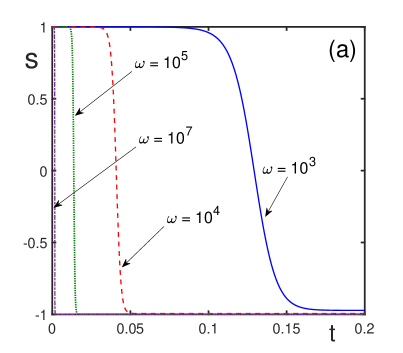
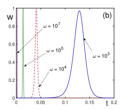
Figure 1: Temporal behavior of the longitudinal spin polarization $s$ (a) and coherence intensity $w$ (b) for $q=0$, $\gamma=10$, and different $\omega$ measured in units of $\gamma_{2}$. Time is measured in units of $1/\gamma_{2}$. The delay time of spin reversals diminishes with increasing $\omega$.

The influence of the quadratic Zeeman effect is illustrated by the numerical solution of Eqs. (82) and (83). When the quadratic Zeeman effect is absent, hence $q=0$, the spin polarization $s$ and coherence intensity $w$ are shown in Fig. 1. In agreement with the above discussion, the delay time of spin reversal diminishes with increasing $\omega$. The spin reversals are accompanied by the pulses of coherence intensity. The coherent motion of spins develops due to the action of the feedback field.

At small, but finite, parameters $q$ and for the frequencies smaller than the critical frequency, the behavior of solutions is similar to the case of zero $q$. However, approaching the critical frequency, the solutions exhibit oscillations after the spin reversal, which is caused by the oscillations in the coupling functions. This is demonstrated in Fig. 2, where for $\omega=10^{3}$ and $\omega=10^{4}$, there occurs a complete spin reversal without oscillations. And for $\omega=10^{5}$, the spin reversal is slightly incomplete and there are oscillations after the reversal. There is no noticeable difference for positive or negative $q=\pm 10^{-8}$. Here and in what follows, the frequencies and attenuations are measured in units of $\gamma_{2}$. Spin reversal time diminishes with increasing $\omega$.

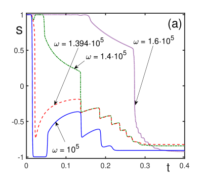
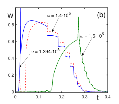
Figure 3: Spin polarization $s$ (a) and coherence intensity $w$ (b) as functions of time, measured in units of $1/\gamma_{2}$, for $q=10^{-8}$, $\gamma=10$ and different frequencies larger than or equal to $\omega=10^{5}$, in units of $\gamma_{2}$. Spin reversal time increases with increasing $\omega$.

For $q=10^{8}$ and the frequencies larger than $\omega=10^{5}$, the spin reversal time increases with increasing $\omega$, as is explained above and as is shown in Fig. 3.

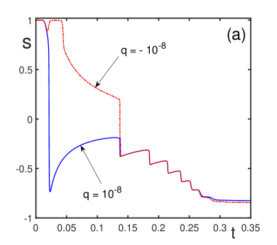
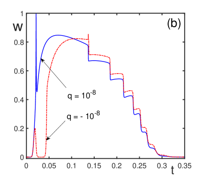
Figure 4: Spin polarization $s$ (a) and coherence intensity $w$ (b) as functions of time, measured in units of $1/\gamma_{2}$, for $\gamma=10$, $\omega=1.394\cdot 10^{5}$, in units of $\gamma_{2}$, and for $q=\pm 10^{-8}$.

In the vicinity of the critical frequency, there appears the dependence on the sign of $q$, as is illustrated in Fig. 4. The spin reversal time is larger for the negative $q$, since, as is seen from Eq. (85), a negative $A$ diminishes the effective coupling parameter $g_{eff}$, hence increases the spin reversal time.

As is demonstrated in Fig. 2, the oscillations in the solutions appear at large frequencies. To realize spin reversal without oscillations, one can proceed as follows. Notice that the oscillations arise due to the oscillating behavior of the coupling functions (67) and (68), which is caused by a nonzero value of the effective detuning $\Delta_{s}$ defined in Eq. (65). It is clear that to make oscillations smaller, it is necessary to diminish the parameter $A$, given in Eq. (76). This parameter combines the terms due to both the static-current quadratic Zeeman effect and alternating-current quadratic Zeeman effect. Since the sign of the alternating-current quadratic Zeeman effect parameter $q_{Z}$, defined in Eq. (9), can be easily varied by varying the detuning $\Delta$, it is possible to make its sign opposite to that of the static-current quadratic Zeeman effect parameter $Q_{Z}$, given in Eq. (8). This reduces the value of the combined parameter $A$, as a result reducing oscillations of the coupling functions (67) and (68). This compensation effect is illustrated in Fig. 5 for small $|A|\ll 1$. Then spin oscillations are suppressed for all frequencies and spin reversal time decreases with increasing $\omega$.

8 Conclusion

We have considered a system of spinor atoms loaded into a deep optical lattice, where atomic degrees of motion are frozen, while effective spin variables can move, being regulated by external magnetic fields. The sample is subject to a static magnetic field and a feedback field of a magnetic coil of a resonance electric circuit. The existence of the feedback field makes it possible to realize a coherent motion of spins leading to a fast spin reversal, when the sample is initially prepared in a strongly nonequilibrium state.

A system of spinor atoms, in addition to the usual linear Zeeman effect, can experience two types of quadratic Zeeman effect, the so-called nonresonant static-current quadratic Zeeman effect and a quasi-resonant alternating-current quadratic Zeeman effect. The influence of both these effects on spin dynamics is studied. Conditions are emphasized, when it is possible to realize fast spin reversal from an initially prepared strongly nonequilibrium state. Such spin reversals can find wide applications in spintronics and information processing.

For concreteness, we have considered spinor atoms, but, we think, the application of the present theory can be much wider. For instance, quantum dots in many aspects are similar to atoms, often being even termed artificial atoms [39]. Quantum dots can also experience quadratic Zeeman effect [40]. A system of quantum dots could be another example of a nontrivial influence of quadratic Zeeman effect on spin dynamics.

Author contribution statement

All authors contributed equally to the paper.

Figure Captions

Figure 1. Temporal behavior of the longitudinal spin polarization $s$ (a) and coherence intensity $w$ (b) for $q=0$, $\gamma=10$, and different $\omega$ measured in units of $\gamma_{2}$. Time is measured in units of $1/\gamma_{2}$. The delay time of spin reversals diminishes with increasing $\omega$.

Figure 2. Time dependence of the spin polarization $s$ (a) and coherence intensity $w$ (b) for $\gamma=10$, $q=\pm 10^{-8}$, and different $\omega$ in units of $\gamma_{2}$. Time is measured in units of $1/\gamma_{2}$. For the frequencies smaller than $\omega=10^{5}$, the time of spin reversal diminishes with increasing $\omega$.

Figure 3. Spin polarization $s$ (a) and coherence intensity $w$ (b) as functions of time, measured in units of $1/\gamma_{2}$, for $q=10^{-8}$, $\gamma=10$ and different frequencies larger than or equal to $\omega=10^{5}$, in units of $\gamma_{2}$. Spin reversal time increases with increasing $\omega$.

Figure 4. Spin polarization $s$ (a) and coherence intensity $w$ (b) as functions of time, measured in units of $1/\gamma_{2}$, for $\gamma=10$, $\omega=1.394\cdot 10^{5}$, in units of $\gamma_{2}$, and for $q=\pm 10^{-8}$.

Figure 5. Longitudinal spin polarization as a function of time measured in units of $1/\gamma_{2}$ for $|A|\ll 1$, $\gamma=10$, $q=\pm 10^{-7}$ and different $\omega$ measured in units of $\gamma_{2}$. Spin reversal time decreases with increasing $\omega$.

                 

                 

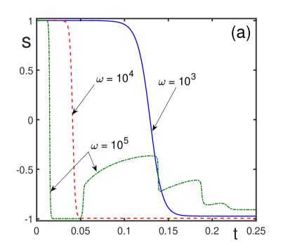
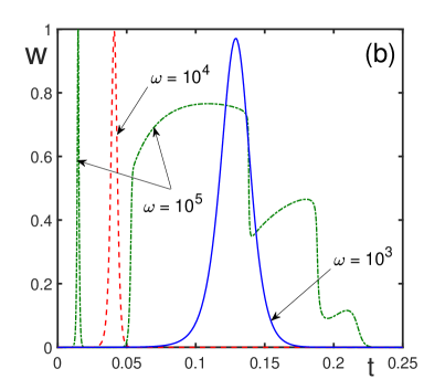
Figure 2: Time dependence of the spin polarization $s$ (a) and coherence intensity $w$ (b) for $\gamma=10$, $q=\pm 10^{-8}$, and different $\omega$ in units of $\gamma_{2}$. Time is measured in units of $1/\gamma_{2}$. For the frequencies smaller than $\omega=10^{5}$, the time of spin reversal diminishes with increasing $\omega$.

                 

                 

Figure 5: Longitudinal spin polarization as a function of time measured in units of $1/\gamma_{2}$ for $|A|\ll 1$, $\gamma=10$, $q=\pm 10^{-7}$ and different $\omega$ measured in units of $\gamma_{2}$. Spin reversal time decreases with increasing $\omega$.

References

- [1] A. Griesmaier, J. Phys. B 40, R91 (2007)
- [2] M.A. Baranov, Phys. Rep. 464, 71 (2008)
- [3] C.J. Pethick, H. Smith, Bose-Einstein Condensation in Dilute Gases (Cambridge University, Cambridge, 2008)
- [4] M. Ueda, Fundamentals and New Frontiers of Bose-Einstein Condensation (World Scientific, Singapore, 2010)
- [5] M.A. Baranov, M, Dalmonte, G. Pupillo, P. Zoller, Chem. Rev. 112, 5012 (2012)
- [6] B. Gadway, B Yan, J. Phys. B 49, 152002 (2016)
- [7] D.M. Stamper-Kurn, M. Ueda, Rev. Mod. Phys. 85, 1191 (2013)
- [8] V.I. Yukalov, E.P. Yukalova, Laser Phys. 26, 045501 (2016)
- [9] V.I. Yukalov, Laser Phys. 28, 053001 (2018)
- [10] F.A. Jenkins, E. Segre, Phys. Rev. 59, 52 (1939)
- [11] L.I. Schiff, H. Snyder, Phys. Rev. 59, 59 (1939)
- [12] J. Killingbeck, J. Phys. B 12, 25 (1979)
- [13] S.L. Coffey, A. Deprit, B. Miller, C.A. Williams, New York Acad. Sci. 497, 22 (1987)
- [14] F. Gerbier, A. Widera, S. Folling, O. Mandel, I. Bloch, Phys. Rev. A 73, 041602 (2006)
- [15] S.R. Leslie, J. Guzman, M. Vengalattore, J.D. Sau, M.L. Cohen, D.M. Stamper-Kurn, Phys. Rev. A 79, 043631 (2009)
- [16] E.M. Bookjans, A. Vinit, C. Raman, Phys. Rev. Lett. 107, 195306 (2011)
- [17] C. Cohen-Tannoudji, J. Dupon-Roc, Phys. Rev. A 5, 968 (1972)
- [18] L. Santos, M. Fattori, J. Stuhler, T. Pfau, Phys. Rev. A 75, 053606 (2007)
- [19] K. Jensen, V.M. Acosta, J.M. Higbie, M.P. Ledbetter, S.M. Rochester, D. Budker, Phys. Rev. A 79, 023406 (2009)
- [20] A. de Paz, A. Sharma, A. Chotia, E. Marechal, J. Huckans, P. Pedri, L. Santos, O. Gorceix, L. Vernac, B. Laburthe-Tolra, Phys. Rev. Lett. 111, 185305 (2013)
- [21] A.K. Jonscher, Universal Relaxation Rate (Chelsea Dielectrics, London, 1996)
- [22] N. Marzari, A.A. Mostofi, J.R. Yates, I. Souza, D. Vanderbilt, Rev. Mod. Phys. 84, 1419 (2012)
- [23] V.I. Yukalov, Laser Phys. 12, 1089 (2002)
- [24] V.I. Yukalov, E.P. Yukalova, Phys. Part. Nucl. 35, 348 (2004)
- [25] V.I. Yukalov, Phys. Rev. B 71, 184432 (2005)
- [26] V.I. Yukalov, Laser Phys. 5, 970 (1995)
- [27] V.I. Yukalov, Phys. Rev. B 53, 9232 (1996)
- [28] V.I. Yukalov, E.P. Yukalova, J. Magn. Magn. Mater. 465, 450 (2018)
- [29] N.G. van Kampen, Stochastic Processes in Physics and Chemistry (North-Holland, Amsterdam, 1981)
- [30] R. Kubo, M. Toda, N. Hashitsume, Statistical Physics (Springer, Berlin, 1985)
- [31] A.S. Mikhailov, Phys. Rep. 184, 307 (1989)
- [32] D. ter Haar, 1977 Lectures on Selected Topics in Statistical Mechanics (Pergamon, Oxford, 1977)
- [33] A. Abragam, M. Goldman, Nuclear Magnetism: Order and Disorder (Clarendon, Oxford, 1982)
- [34] N.N. Bogolubov, Y.A. Mitropolsky, Asymptotic Methods in the Theory of Nonlinear Oscillations (Gordon and Breach, New York, 1961)
- [35] M.I. Freidlin, D.A. Wentzell, Random Perturbations of Dynamical Systems ( Springer, New York, 1998)
- [36] J.A. Morrison, J. McKenna, in Stochastic Differential Equations, edited by J.B. Keller, H.P. McKean (Am. Math. Soc., Providence, 1973), p. 97
- [37] C. Frapolli, T. Zibold, A. Invernizzi, K.J. Garcia, J. Dalibard, F. Gerbier, Phys. Rev. Lett. 119, 050404 (2017).
- [38] I.S. Grigoriev, E.Z. Meilikhov, eds. Handbook of Physical Quantities (CRC, Boca Raton, 1996)
- [39] J.L. Birman, R.G. Nazmitdinov, and V.I. Yukalov, Phys. Rep. 526, 1 (2013)
- [40] S.J. Prado, C. Trallero-Giner, A.M. Alcalde, V. Lopez-Richard, G.E. Marques, Phys. Rev. B 67, 165306 (2003)