The z=0.54 LoBAL Quasar SDSS  J085053.12+445122.5: II. The Nature of Partial Covering in the Broad-Absorption-Line Outflow

Abstract

It has been known for 20 years that the absorbing gas in broad absorption line quasars does not completely cover the continuum emission region, and that partial covering must be accounted for to accurately measure the column density of the outflowing gas. However, the nature of partial covering itself is not understood. Extrapolation of the SimBAL spectral synthesis model of the HST COS UV spectrum from SDSS J0850+4451 reported by Leighly et al. (2018) to non-simultaneous rest-frame optical and near-infrared spectra reveals evidence that the covering fraction has wavelength dependence, and is a factor of 2.5 times higher in the UV than in the optical and near-infrared bands. The difference in covering fraction can be explained if the outflow consists of clumps that are small and either structured or clustered relative to the projected size of the UV continuum emission region, and have a more diffuse distribution on size scales comparable to the near-infrared continuum emission region size. The lower covering fraction over the larger physical area results in a reduction of the measured total column density by a factor of 1.6 compared with the UV-only solution. This experiment demonstrates that we can compare rest-frame UV and near-infrared absorption lines, specifically He I*$\lambda 10830$, to place constraints on the uniformity of absorption gas in broad absorbing line quasars.

1 Introduction

Broad absorption lines are found in the rest-frame UV spectra of a significant fraction of quasars (e.g., Weymann et al., 1991; Gibson et al., 2009). Most often, these lines are blueshifted with velocities as high as tens of thousands $\rm km\,s^{-1}$, indicating the presence of powerful outflows. Optical spectra of $z\sim 2$ broad absorption line quasars (BALQs) include absorption lines from Ly$\alpha$, N V, Si IV, and C IV, among others. Early on, scientists recognized that it might be possible to use these lines to determine the metallicity of the outflowing gas, thereby potentially constraining the physical conditions in the quasar central regions and the potential for enrichment of the IGM (see Hamann, 1998, and references therein). However, they quickly discovered that the implied metallicities were enormous (e.g., 20–100 times solar; Hamann, 1998). Especially problematic were quasars with P V$\lambda 1118,1128$ absorption lines, as phosphorus is a relatively rare element with an abundance only $9.3\times 10^{-4}$ that of carbon (Grevesse et al., 2007). Hamann (1998) proposed that, instead, the absorber only partially covers the continuum source, so that an absorption line from a high-abundance ion such as C⁺³ can be completely saturated without dropping to zero flux density, and a low-abundance ion such as P⁺⁴ can show significant optical depth.

Additional support for partial covering comes from doublet analysis in objects with relatively narrow absorption lines. The ratios of opacities of absorption lines from the same lower level are fixed by atomic physics. For example, due to the fine structure of the upper level, the C IV absorption line at 1548Å (upper level configuration ${}^{2}P_{3/2}$, with degeneracy 4) will have approximately twice the opacity of the line at 1550Å (upper level configuration ${}^{2}P_{1/2}$, with degeneracy 2). If the apparent opacities are less than 2:1, then the presence of partial covering is inferred (e.g., Hamann et al., 2001). In fact, partial covering is routinely used to distinguish narrow absorption lines (NALs) intrinsic to the quasar from absorption lines from intervening gas which would completely cover the continuum source (e.g., Misawa et al., 2007; Rodríguez Hidalgo et al., 2011; Ganguly et al., 2013).

The spectropolarimetric properties of BALQs also provide evidence for partial covering. Often, the polarization is stronger in the BAL troughs of polarized BALQs (Ogle et al., 1999; DiPompeo et al., 2013), indicating that at least in some cases, scattered light fills in the troughs, or at least contributes to the continuum in the trough.

Once partial covering was recognized to be nearly ubiquitous in quasars, investigators set about trying to account for it. Fortunately, many of the most prominent absorption lines come from lithium- or sodium-like ions (e.g., C⁺³, N⁺⁴, O⁺⁶, Mg⁺, Al⁺², Si⁺³, P⁺⁴, Ca⁺); all of these ions share the atomic structure discussed above for C⁺³, namely, a doublet transition from the ground state, with the optical depth ratios of 2:1 fixed by atomic physics. Optical depth measurements of both lines yield two equations for two unknowns (the covering fraction and the optical depth), implying that the true optical depth could be solved for exactly (e.g., Hamann et al., 2001). This method works well (e.g., Arav et al., 2005, 2008; Borguet et al., 2012, 2013; Chamberlain et al., 2015; Dunn et al., 2010; Finn et al., 2014; Gabel et al., 2005; Hamann et al., 1997, 2001, 2011; Hall et al., 2003; Moravec et al., 2017; Moe et al., 2009; Rodríguez Hidalgo et al., 2011) as long as both lines are not saturated. The fact that the optical depths are 2:1 means that these lines have a rather limited dynamic range in optical depth over which they are useful. Leighly et al. (2011) discussed a potentially very useful set of lines that arise from metastable helium, especially He I*$\lambda 10380$, the $2S\rightarrow 2P$ transition, and He I*$\lambda 3889$, the $2S\rightarrow 3P$ transition, which have an opacity ratio of 23:1. This high ratio makes these lines ideal for very high column density outflows, which are potentially the most interesting for identifying quasar activity that is likely to affect the host galaxy. The true column density of hydrogen can be estimated using the Lyman series lines (e.g., Gabel et al., 2005), although this can be difficult in cases where the Ly$\alpha$ forest is present and blended with the absorption lines of interest as is generally the case for quasars found at the epoch of peak quasar activity ($z=1$–3).

The partial covering analysis discussed above implicitly assumes that part of the continuum emission region is completely covered and the other part is completely bare. This “step function” (Arav et al., 2005) partial covering is not the only possibility, and indeed, early on it was recognized that abundant ions tended to have higher covering fractions than lower abundance ions (Hamann et al., 2001). A popular second model, called the inhomogeneous absorber (de Kool et al., 2002; Arav et al., 2005) or the power-law partial covering model (Arav et al., 2005; Sabra & Hamann, 2005), posits that the optical depth has a power-law distribution over the continuum emission region. The power-law partial covering model can naturally account for the difference in apparent covering fractions among ions. The step function and power-law partial covering models can be distinguished if there are more than two absorption lines from the same lower level, and detailed analysis shows that the inhomogeneous absorber model is sometimes preferred (de Kool et al., 2002; Arav et al., 2005).

Most of these analyses ignore the interesting question of the physical origin of partial covering. Absorption lines are observed along the line of sight to the continuum emission region in the central engine. From the point of view of an observer on Earth, the continuum emission region is spatially unresolved. But from the point of view of the absorber, the continuum emission region may be spatially resolved. Moreover, the continuum emission is assumed to come from an accretion disk, hotter in the center and cooler at larger radii, which means that the continuum emission region is resolved as a function of wavelength too. For example, a simple sum-of-blackbodies accretion disk model has radial temperature dependence $T\propto R^{-3/4}$. Therefore it is possible that the absorber, located in the vicinity of the torus at $\sim 1\rm\,pc$, for example, may present a higher covering fraction to the hot and compact central part of the accretion disk than to cooler parts at larger radii. Therefore, the covering fraction measured in the UV bandpass refers to a much smaller continuum emission region than the covering fraction in the optical and near-infrared bands. Analysis of partial covering as a function of wavelength would lead to an enhanced understanding of the geometry of the absorber in BALQs as well as constrain the relative angular sizes of the continuum emission regions as a function of wavelength. So, instead of only obtaining information along a single radial sight line, we would be able to investigate the angular distribution as well. A caveat is that we assume that negligible flux is scattered into our line of sight.

To do this experiment, we clearly need to analyze lines widely separated in wavelength to probe different size scales of the accretion disk. However, we cannot obtain this information from just any pair of absorption lines, due to the fact that abundant ions have higher covering fractions than less abundant ions: the pair of lines should have about the same optical depth in the gas. Leighly et al. (2011) showed that this criterion is fulfilled over a wide range of physical conditions by P V$\lambda\lambda 1118,1128$ and the metastable helium lines, in particular He I*$\lambda 10830$. These two lines probe dramatically different size scales of the accretion disk; for the sum-of-blackbodies model (e.g., Frank et al., 2002), the radius of the accretion disk emitting at 1 micron is a factor of 12 times larger than the radius of the accretion disk emitting at 1100Å (see §6.2). In terms of area, this corresponds to a factor of 140, i.e., dramatically different size scales.

The low redshift ($z=0.5422$) LoBAL quasar SDSS J085053.12$+$445122.5, hereafter referred to as SDSS J0850+4451, was discovered to have a He I*$\lambda 3889$ absorption line in its SDSS spectrum (e.g., Luo et al., 2013). We obtained Gemini GNIRS and LBT LUCI near-infrared spectroscopic observations and identified the presence of a deep He I*$\lambda 10830$ absorption line (§2 below). SDSS J0850$+$4451 was detected by GALEX, indicating that it was bright enough to be observed by HST using COS. The COS spectral analysis was described in Leighly et al. (2018), hereafter Paper I, using a novel spectral synthesis program called SimBAL. The results of that analysis are summarized in §4.1. We extrapolated the SimBAL best-fitting solutions to the optical and near-IR, finding that the predicted absorption was significantly deeper than observed (§4.2), and therefore apparently indicated differential partial covering. The HST and near-IR observations were not simultaneous, and we investigate the potential impact of variability on our result in Appendix A. In addition, the host galaxy emits strongly at 1 micron, i.e., under the He I*$\lambda 10830$ absorption line, so we performed spectral energy distribution (SED) fitting and image analysis to show that the contribution of the host galaxy to the 1-micron continuum is negligible and is therefore not filling in the absorption line (Appendix B). A quantitative analysis of the difference in covering fraction in the UV, optical, and near-IR is reported in §4.3, and an analysis of the difference in the covering fraction between the continuum and broad emission lines is discussed in §4.4. A discussion of the nature of the power-law covering-fraction parameterization is given in §5. The implications of our results on our understanding of the physical properties of partial covering are discussed in §6, and the summary of our principal results is given in §7. Vacuum wavelengths are used throughout. Cosmological parameters used depend on the context (e.g., when comparing with results from an older paper), and are reported in the text.

2 Observations and Data Reduction

We report data from taken at six different observatories. We obtained near-IR spectra at Gemini (§2.1) and LBT (§2.2) to measure the properties of the He I*$\lambda 10830$ line. To mitigate against absorption-line variability confounding the He I* analysis, we obtained new optical spectra at MDM observatory (§2.4) contemporaneous with the near-IR observations, as well as near-IR photometry to estimate the host galaxy contribution through SED fitting. Subsequent optical spectra obtained at APO (§2.6) and KPNO (§2.3), combined with the SDSS and BOSS spectra (§2.5), were used to track absorption-line variability. The log of all of the observations of SDSS J0850$+$4451 analyzed in this paper is given in Table 1.

Table 1: Observations of SDSS J0850$+$4451

Observatory and Instrument	Date	Exposure	Rest Frame Band Pass or	Resolution
		(s)	Effective Wavelength (Å)
SDSS	2002 Nov 27	9000.0	2472–5975	$100\rm\,km\,s^{-1}$
HST (WFC3 IR)	2010 April 9	905.9	12500	0.13 arc sec/pixel
LBT (LUCI)	2010 Dec 12	1500.0	9512–15304	$160\rm\,km\,s^{-1}$
MDM (CCDS)	2011 Feb 11	9600.0	3121–4108	$210\rm\,km\,s^{-1}$
Gemini (GNIRS)	2011 Apr 23, 24; 2011 Jun 6	1520.0	5513–16466	$240\rm\,km\,s^{-1}$
MDM (TIFKAM)	2012 Dec 29	990, 720, 720	8105, 10700, 14265	1.0 arcsec
APO (DIS)	2014 Apr 12	4500.0	2206–6353	380, $400\rm\,km\,s^{-1}$
BOSS	2015 Jan 20	3600.0	2345–6740	$89\rm\,km\,s^{-1}$
KPNO (KOSMOS)	2015 Apr 24	3600.0	3804–6631	$120\rm\,km\,s^{-1}$

2.1 Gemini GNIRS Observations

SDSS J0850$+$4451 was observed using GNIRS on the Gillett Gemini Telescope using a standard cross-dispersed mode (the SXD camera with the $31.7\rm\,l/mm$ grating) and a $0{\farcs}45$ slit. Observations were made on 23 April 2011, 24 April 2011, 26 May 2011, and 7 June 2011. The 26 May observation was deemed unusable due to detector noise, as the detector read mode had been mistakenly set at “Very Bright/Acq./High Bckgrd”, rather than “Very Faint Objects” mode. On 23 April 2011, $8\times 190$ second exposures were made, in an ABBA pattern. On 24 April 2011, $8\times 190$ second exposures were made, in an ABBA pattern. On 6 June 2011, $4\times 190$ second exposures were made, also in an ABBA pattern. A0 stars were observed at approximately the same airmass and adjacent to the object observation for telluric correction. The data were reduced using the IRAF Gemini package, coupled with the GNIRS XD reduction scripts, in the standard manner for near-infrared spectra, through the spectral extraction step. For telluric correction, the Gemini spectra of the source and the telluric standard star were converted to a format that resembled IRTF SpeX data sufficiently that the Spextool xtellcor package (Cushing et al., 2004; Vacca et al., 2003) could be used.

2.2 LBT Observation

SDSS J0850$+$4451 was observed using LBT LUCI on 12 December 2010. Six exposures were made, with the object offset along the slit between each observation. An A0 star was observed adjacent to the target observation at approximately the same airmass. There is no reduction pipeline for LUCI data, so the data were reduced by hand using IRAF. Because the target was much fainter than the sky lines, special care was taken to straighten the object trace and sky lines. Wavelength correction was obtained using sky lines. The telluric correction was performed using xtellcor_general, the generalization of the xtellcor procedure for 1-D (versus cross-dispersed) spectra (Cushing et al., 2004; Vacca et al., 2003).

The LBT spectrum and the three Gemini spectra were combined. First, the four spectra were resampled onto a common wavelength range, and averaged without weighting. The GNIRS spectrum obtained on 23 April 2011 appeared to have the best signal-to-noise ratio and the best calibration, and the other spectra were normalized and tilted to conform with that one.

In §6.3, we discuss an LBT observation of the quasar PG 1254$+$047. It was observed using LBT LUCI on 2013 Jan 3 for 960 seconds in eight exposures using an ABBA configuration. The A0 telluric star HD 116960 was observed immediately after the PG 1254$+$047 observation in four 12-second exposures for a total of 48 seconds. Standard methods for extraction and wavelength calibration were done using IRAF. The telluric correction was done using IRTF xtellcor_general (Vacca et al., 2003).

2.3 KPNO Observation

We obtained $3\times 1200\rm\,s$ optical spectra of SDSS J0850$+$4451 on the night of UT 24 April 2015 using the KOSMOS spectrograph (Martini et al., 2014) on the Mayall Telescope at the Kitt Peak National Observatory. We employed the blue VPH grism and center slit, which yielded spectra from 3804 – 6631Å at 0.69 Å ${\rm pixel}^{-1}$. The slit width was $0{\farcs}9$, and typical seeing was about $1{\farcs}2$. The resolution of the spectra, as measured by telluric emission lines, was 2.6 pixels at the center of the spectra and 2.8 pixels at either end.

The output images of the spectrograph had dimension $320\times 4096$ pixels, read out through two amplifier sections of size $160\times 4096$ pixels. All the data were contaminated by fixed pattern noise which was symmetric on the two amplifiers. The spectra were positioned along the slit so that they fully fell on one amplifier. The first step in the data processing was to apply an overscan correction on each amplifier, and then to remove the pattern noise by flipping the image section from the side not containing the spectrum and then subtracting it from the side that did. This also partially subtracted the night sky lines, which extended across both amplifiers. Other calibration steps were the subtraction of zero-exposure frames and the application of flat-field corrections; the latter were constructed from a combination of quartz lamps in the spectrograph and lamps illuminating a white spot on the inside of the telescope dome. After flat fielding, cosmic rays in the sky regions of the image were removed by hand using a filter that replaced pixel values more than 5$\sigma$ from the median with the median value. After cosmic-ray cleaning, the three exposures were averaged and the spectrum extracted in the usual fashion. Noise as a function of counts in the spectrum was estimated from the scatter after subtracting a highly smoothed spectrum. The spectrum was flux calibrated using observations of Feige 34 that were taken the same night as SDSS J0850$+$4451.

2.4 MDM Observations

SDSS J0850$+$4451 was observed using the Boller & Chivens CCD Spectrograph (CCDS) on the Hiltner 2.4m telescope at MDM observatory on 11 Feb 2011 under photometric conditions. Eight 20-minute observations were made. The data were reduced in a standard manner using IRAF.

SDSS J0850$+$4451 is a relatively faint target for 2MASS; the quality flags associated with this in the catalog are “BCB” indicating that the H band photometry is especially uncertain. Therefore, we also obtained deep JHK imaging observations in order to obtain the photometry for SED fitting with the goal of constraining the contribution of the host galaxy to the near-UV continuum (§B.1). We used TIFKAM (Depoy et al., 1993) at the 2.4m Hiltner Telescope of the MDM observatory. We employed the f/5 reimaging camera, which delivered a field 5.1 arcmin over 1024 pixels at a frame scale of $0\farcs 30\ {\rm pixel}^{-1}$. About 10% of each frame was slightly vignetted from an out-of-alignment internal baffle, but this was corrected in the reduction process.

The observations were obtained on the night of UT 2012 December 29. For each filter, we obtained a series of 90-second exposures with position offsets varied irregularly between exposures. The total exposure time in $J$ was 990 seconds, while in $H$ and $K$ the total was 720 seconds. After a small linearity correction, the pixel values in the images from each filter were scaled and then combined by a median to produce a sky frame; this was also corrected for dark current to generate a flat field. The corrected images were then combined by averaging to produce master images in each of $JHK$. Photometry of SDSS J0850$+$4451 was derived from these combined images with respect to the 2MASS catalog values for the other objects on each frame, which were almost always brighter than SDSS J0850$+$4451. SDSS J0850$+$4451 is one of the reddest objects in the nearby field, but its $J-H$ and $J-K$ colors are within the range spanned by the other objects. Evidence for significant color terms in the transformation to the 2MASS system was marginal, so in the end we derived a simple constant offset to transform from the instrumental TIFKAM “m” to 2MASS “M” magnitudes: $M=m+{\rm const}$. Errors in the photometry were derived from the standard deviation of the magnitudes on individual frames and propagation of the 2MASS catalog error values. The final values from our photometry were $J=16.202\pm 0.024$, $H=15.507\pm 0.023$ and $K=14.763\pm 0.028$.

2.5 SDSS and BOSS Spectra

SDSS J0850$+$4451 was observed using SDSS on 27 Nov 2002. The MDM and SDSS spectra had very similar emission and absorption lines, so they were averaged over the segment including the He I*$\lambda 3889$ line, in order to increase signal-to-noise ratio, after the MDM spectrum was tilted and scaled to match the SDSS spectrum.

SDSS J0850$+$4451 was observed again using BOSS on 20 Jan 2015. As will be discussed in §A.1, the continuum shows an unusual shape at the blue end of the spectrum (Fig. 3). Because this observation was made relatively close in time to the KPNO observation (within 3 months), and since the KPNO shows no such unnatural shape, we suspect that a calibration problem is responsible rather than a real change in continuum shape. Note that this should not be the atmospheric differential refraction problem known to plague the BOSS spectrograph (Margala et al., 2016) as correction for that issue was included in the DR14 pipeline.

2.6 APO Observation

We obtained spectra on the night of UT 2014 April 12 using the Dual Imaging Spectrograph (DIS) spectrograph on the ARC 3.5m telescope at the Apache Point Observatory. This two-channel spectrograph uses a dichroic to simultaneously obtain spectra in a blue and red channel. On the blue side we used the B400 grating, which delivered spectra from 3402–5564 Å at a dispersion of $1.82$ Å pixel^-1; the red side used the R300 grating, yielding spectra from 5281–9796Å at 2.66Å pixel^-1. We observed with a $1\farcs 5$ wide slit. The dispersed images in both channels underfill the CCD detectors spatially, so these wavelength ranges were set by determining the regions where the locations of the SDSS J0850$+$4451 spectrum could reliably be traced. The wavelength solution is not reliable for the first and last $\sim 100$ Å of each spectrum because of a lack of arc lamp lines near the edges of each image. The spectral resolution on the blue and red sides was 3.0 and 2.9 pixels FWHM, respectively. Image processing and spectral extraction were performed using the same techniques as for the KPNO spectra. Flux calibration was determined using spectra of Feige 34 obtained near in time to the SDSS J0850$+$4451 spectra.

3 Continuum Modeling

Our focus in this paper is on the absorption lines. Therefore, we model the continuum with several components including the emission lines and divide by the result before performing the absorption-line modeling. As in Paper I, we first correct the spectrum for Milky Way reddening using $E(B-V)=0.024$ (Schlafly & Finkbeiner, 2011), and for the cosmological redshift $0.5422$, estimated from the narrow [O III] line in the SDSS spectrum.

The SDSS J10850$+$4451 near-infrared continuum shows the characteristic break between the optical power law originating in the accretion disk and the near-infrared bump due to hot dust. We used Sherpa (Freeman et al., 2001) to model the entire continuum spectrum using a power law for the accretion disk continuum and a black body for the thermal dust emission, plus a modest contribution from Paschen recombination continuum near 8000Å. Both H$\alpha$ and Pa$\beta$ are present in the spectra. Both of these lines could be modeled with two Gaussians. H$\alpha$ is somewhat broad and mostly symmetric, while Pa$\beta$ is very broad with a prominent blue wing. Pa$\delta$ was also fit well with the same profile as Pa$\beta$. In the vicinity of the He I*$\lambda 10830$ absorption line, the principal emission lines are He I*$\lambda 10830$, and Pa$\gamma\,\lambda 10941$, plus some low-level emission longward of Pa$\gamma$, possibly attributed to O I$\lambda 11290$. We found that we could only obtain a satisfactory fit if He I*$\lambda 10830$ has a shape more similar to H$\alpha$, i.e., as two Gaussians with FWHM and wavelength tied to the H$\alpha$ parameters, but with the flux free to vary, plus a narrower He I* component with FWHM $1210\rm\,km\,s^{-1}$. It must be noted that a prominent sky line falls at the wavelength of the putative narrow component, so the properties and necessity of that component are uncertain. The resulting fit is shown in Fig. 1.

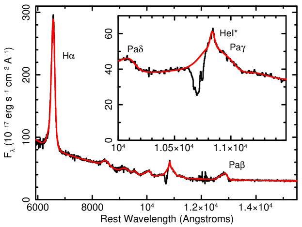
Figure 1: The combined Gemini GNIRS and LBT LUCI spectrum of SDSS J0850+4451, fitted with a continuum plus emission lines model (red curve). The inset shows the bandpass that includes the He I*$\lambda 10830$ absorption line. Principal emission lines are marked.

The combined SDSS and MDM spectrum (Fig. 2) shows that SDSS J0850$+$4451 is a broad-line AGN with modest, broadened Fe II emission. The absorption lines are easily identified against the continuum. For the blue optical wavelengths, we used the composite Fe II spectra developed in Leighly et al. (2011). For the region around Mg II, we used an Fe II emission spectrum extracted by us from the HST observation of I Zw 1 (Leighly & Moore, 2006). Both were convolved with a Gaussian with a width of $2000\rm\,km\,s^{-1}$. We modeled the spectrum with the broad Fe II, a broken power law, a small amount of Balmer continuum, and broad Gaussians for the Mg II emission lines, as well as broad Gaussians for H$\delta$ and He II$\lambda 4865$. This continuum isolates the He I*$\lambda 3889$, He I*$\lambda 3188$, and Mg II absorption lines (Fig. 2).

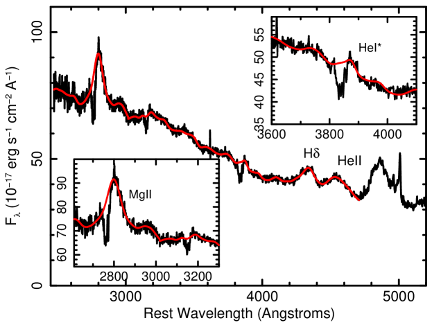
Figure 2: The combined SDSS and MDM spectrum of SDSS J0850+4451, fitted with a continuum model (red curve). The insets show the bandpasses that include the He I*$\lambda 3889$ (upper right), and Mg II and He I*$\lambda 3188$ absorption lines (lower left). Principal emission lines are marked.

4 Partial Covering Absorption in SDSS J0850$+$4451

4.1 Summary of Paper I

The goal of the multi-wavelength observations of SDSS J0850$+$4451 was to investigate the nature of partial covering in this object. In Paper I, we described the analysis of the HST COS spectrum of SDSS J0850$+$4451 using our novel spectral synthesis code SimBAL. We briefly review the most relevant aspects of that analysis and the results to set the stage for the partial-covering analysis described in this paper.

The SimBAL analysis method uses large grids of ionic column densities extracted from Cloudy (Ferland et al., 2013) models to create synthetic spectra as a function of velocity, covering fraction, ionization parameter, density, and a combination parameter $\log N_{H}-\log U$. We use the Markov Chain Monte Carlo code emcee (Foreman-Mackey et al., 2013) to compare the continuum-normalized HST spectrum with the synthetic spectra, using $\chi^{2}$ as the likelihood estimator. The results of the modeling process are posterior probability distributions of the model parameters, which were used to construct the best-fitting model spectrum and its uncertainties, and to extract best-fitting model parameters and uncertainties. From these, the physical parameters of the outflow, including the total column density, mass outflow rate, momentum flux, and kinetic luminosity were derived.

We developed an innovative method to model the velocity dependence of the outflow parameters. We divided the trough into a specified number of velocity bins, where each bin is required to have the same width, but the physical parameters of the gas were allowed to vary in each bin. The central velocity of the highest-velocity bin and the bin width were fitted parameters. For SDSS J0850$+$4451, we ran models with from 7 to 12 bins in order to investigate systematic uncertainty associated with the number of bins; we found that the dependence on number of bins is small. In addition, we considered two models for the continuum that differ somewhat in the modeling of the Ly$\alpha$ and N V emission line region; see Paper I for details. We considered two Cloudy input spectral energy distributions, a relatively soft one that may be characteristic of quasars (Hamann et al., 2011), and a hard one that may be more suitable for Seyferts (Korista et al., 1997). Finally we considered two cases for the metallicity, solar and $Z=3Z_{\odot}$, both for the soft SED. For the enhanced metallicity models, we followed Hamann et al. (2002): all metals were set to three times their solar value, while nitrogen was set to nine times the solar value, and helium was set to 1.14 times the solar value. As discussed in Paper I, the results were largely independent of these differences in models.

A number of results were robust to variations in our models. The trough spans $-6000$ to $-1000\rm\,km\,s^{-1}$. We found significant structure in $\log N_{H}-\log U$ as a function of velocity, namely an enhancement in the column density by a factor of three around $-4000\rm\,km\,s^{-1}$. We refer to the this velocity-resolved feature as “the concentration”. Both the ionization parameter and the column density were larger at higher speeds. The covering fraction showed a strong decrease with speed.

We estimated the bulk properties of the outflow from our results. The total column density of the outflowing gas $\log N_{H}$ lay between $22.4$ and $22.9\rm\,cm^{-2}$, depending on the metallicity ($Z=3Z_{\odot}$ and solar, respectively). The density-sensitive line C III*$\lambda 1175$ constrained the distance of the outflow from the continuum-emission region to be between 1 and 3 parsecs. C III*$\lambda 1175$ arises from three fine-structure levels, each of which has its own critical density (e.g., Gabel et al., 2005, Fig. 5). While the $J=0$ level is populated at relatively low densities, the $J=1$ becomes significantly populated toward $\log n=6\rm\,[cm^{-3}]$, increasing the opacity of the transition significantly. Assuming that the whole outflow (i.e., including the velocity bins that were not represented in the C III* line) lies at approximately the same distance from the central engine, we found that the mass outflow rate is 17–28 solar masses per year, the momentum flux is approximately equal to $L_{Bol}/c$, and the ratio of the kinematic to bolometric luminosity is 0.8–0.9%. This range is greater than 0.5% (Hopkins & Elvis, 2010), generally taken to be the lower bound required for a quasar outflow to effectively contribute to quasar feedback in galaxy evolution scenarios. The ability to model the velocity dependence of physical properties, as well as extract the global outflow properties illustrates the power of the forward-modeling methodology used by SimBAL.

4.2 Extrapolation to Longer Wavelengths

In the near UV and optical spectrum, we observe absorption lines from Mg II, He I*3188, and He I*3889 (Fig. 2). In the near-infrared spectrum, we observe He I*10830 (Fig. 1). We extrapolated best-fitting models from Paper I to longer wavelengths. As the solutions were largely independent of the number of bins, we chose the 11-bin models from Paper I as representative, and plot the results for the nominal soft SED, the hard SED, and the higher metallicity (and nominal soft SED) for each continuum model. The flux-density median model spectra are shown in Fig. 3.

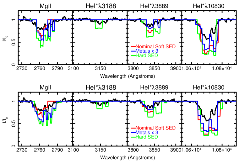
Figure 3: The median spectra from the parameter posterior distributions for the 11-velocity-bin model fitted to HST spectrum and extrapolated to longer wavelengths. The top panel shows the results using the first continuum model, and the lower panel shows the results using the second continuum model, characterized by stronger Ly$\alpha$ emission (see Paper I for details). While the overall correspondence between the shapes of the profiles is good (in particular, the “mitten” shape for He I*$\lambda 10830$), the model over-predicts the absorption line depth for the Mg II and He I* lines, especially for the He I*$\lambda 10830$ line.

This figure shows that the model that fits the UV over-predicts the Mg II and He I* opacity. Generally speaking, the hard SED produces the worst fit, predicting far more opacity for all three lines than observed. This is because a harder SED produces a thicker (e.g., Casebeer et al., 2006, Fig. 13) and hotter (e.g., Leighly et al., 2007, Fig. 14) H II region; He I* shows a mild dependence on temperature (Clegg, 1987). The enhanced metallicity model fits the He I*$\lambda 3889$ line rather well, but it over-predicts the Mg II absorption. All models predict much more absorption at He I*$\lambda 10830$ than is observed.

At first glance, this result might imply that the covering fraction of the longer wavelength continuum emission region is lower than that of the shorter wavelength continuum emission region. This would allow more continuum emission to reach the observer, producing a shallower line. However, there are two factors that we needed to consider before we could draw this conclusion. First, it turns out that SDSS J0850+4451 has demonstrated absorption line variability, and our ground-based optical and near-infrared observations were not simultaneous with the HST observation. We explore the potential effects of variability on our experiment in Appendix A. We conclude that variability is unlikely to have caused the difference between the observed line depths and the extrapolated model line depths, although we cannot rule it out absolutely. Second, the He I*$\lambda 10830$ line is located near 1 micron, the region of the spectrum where the host galaxy is the brightest. So it is conceivable that the continuum is diluted by the presence of the host galaxy, making the line appear shallower than it is. We explore this possibility in Appendix B. We conclude that the host galaxy contribution to the continuum under the He I*$\lambda 10830$ line is negligible.

4.3 Quantifying the Difference in Partial Covering

Having established that the difference in partial covering implied from the extrapolated best-fitting UV spectrum is not an artifact of variability or host galaxy contamination, we proceeded to investigate it quantitatively. As described in Paper I, we parameterized the partial covering using a power law, where $\tau=\tau_{max}x^{a}$. Here, $\tau$ is the integrated opacity of the line, and $\tau_{max}$ is proportional to $\lambda f_{ik}N({\rm ion})$, where $\lambda$ is the wavelength of the line, $f_{ik}$ is the oscillator strength, $N({\rm ion})$ is the ionic column density (e.g., Savage & Sembach, 1991), $x\in(0,1)$ represents the fractional surface area, and $a$, or more specifically $\log a$, is the parameter that is modeled. We chose this formalism because we compute the model spectrum line by line, and we require a scheme that is mathematically commutative. The power-law partial-covering model has been explored by de Kool et al. (2002); Sabra & Hamann (2001); Arav et al. (2005), and in several cases is has been found to provide a better fit than the step-function partial covering model (de Kool et al., 2002; Arav et al., 2005).

As discussed in Paper I, the power-law covering fraction has the property that the fraction of the continuum covered depends on the opacity of the line, which means that the residual intensity can vary dramatically among lines with different opacity for the same value of $a$. So a particular value of $\log a$ will produce lines that are nearly black for a common ion, and lines that are quite shallow for a rare ion. In addition, as discussed by Sabra & Hamann (2001, e.g., their Fig. 1), a value of $a$ equal to 1 ($\log a=0$) corresponds to 50% coverage (for a line with total opacity equal to 1), while $a$ approaching zero corresponds to full coverage, and high values of $a$ correspond to a small fraction covered. Thus, the fitting parameter $\log a$ has an inverse behavior: it is smaller for a larger fraction covered, and larger for a smaller fraction covered. See §5 for further discussion of inhomogeneous partial covering and the power law parameterization.

To investigate the difference in covering fraction between the UV and the long-wavelength spectrum, we performed a SimBAL analysis of the continuum-normalized spectrum between 2500–4200Å and 9000–11500Å. We made the assumption that, of all the variables required in the SimBAL analysis of the HST COS spectrum, only the covering fraction varies. As discussed in Paper I, the resulting physical parameters of the outflow depend little on the number of bins used to span the line profile, so we present the results for the 11-bin case. The variable parameters in this analysis were the 11 values of $\log a$, i.e., the log of the covering fraction index as a function of velocity. The results are shown in Fig. 4. The left panel shows, for reference, the results from fitting the full model to the UV data from Paper I. The partial covering parameter $\log a$ is plotted as a function of velocity for the 11-bin model for 6 combinations of continuum model, SED, and metallicity. The error bars show the 95% confidence intervals from the posterior distributions obtained for each of the model parameters. The middle panel shows the results for the fits of covering fraction at optical and near-IR wavelengths. The $\log a$ is clearly shifted to larger values, indicating a lower covering fraction. The median models overlaid on the data are shown in Fig. 5. While the reduced $\chi^{2}$ for the extrapolated models shown in Fig. 3 ranged from 1.6 to 3.3, indicating an unacceptable fit, the reduced $\chi^{2}$ for these models are all less than 1, indicating an acceptable fit. Physically, this result implies that the covering fraction along the line of sight to the optical and near-IR continuum emission region is lower than the covering fraction along the line of sight to the UV continuum emission region.

We have measured the difference between the covering fractions in the UV and the optical through infrared bands. In principle, there could be a continual decrease in covering fraction as a function of wavelengths. We tried to detect a difference in covering fraction between the three bands: UV, optical (i.e., Mg II and He I*$\lambda 3889$) and the infrared (He I*$\lambda 10830$). We were unable to obtain any useful constraints because of limitations of the data; specifically, the lines are rather shallow and the signal-to-noise ratios are moderate.

To quantify the difference between the covering fractions in the UV and at longer wavelengths, we fit a constant model to $\log a$ as a function of velocity for each of the six models. The $\log a$ varies as a function of velocity, and is not well constrained at low and high velocities where the absorption line is shallow, so we limited the fitting to range between $-4500\rm\,km\,s^{-1}$ and $-1500\rm\,km\,s^{-1}$. Computing the power of 10 of the resulting average values of $\log a$ results yields six estimates of $a$ each for the UV models and the long wavelength models respectively.

How do we interpret the differences in $a$ between the UV and the long wavelengths? We want to know how much more of the continuum emission source is covered in the UV compared with near-infrared and optical wavelengths. To determine this, we return to the definition of the power law covering fraction, $\tau=\tau_{max}x^{a}$, where $0<x<1$ represents the fractional surface area, and ask, at a particular value of $x$, what is the ratio of the fraction covered? Solving this equation for $x$ yields $x=(\tau/\tau_{max})^{1/a}$, and the fraction covered for a particular value of $\tau/\tau_{max}$ is given by $1-(\tau/\tau_{max})^{1/a}$. So in terms of $x$, we want to determine

$$\frac{f_{UV}}{f_{long}}=\frac{1-(\tau/\tau_{max})^{1/a_{UV}}}{1-(\tau/\tau_{max})^{1/a_{long}}}$$

where the “long” subscript refers to the optical through infrared wavelengths. A limiting value is given by $\tau\to\tau_{max}$, but the ratio becomes indeterminate. It turns out that the ratio of the fractions covered approaches the ratios of the $a$ values as $\tau$ approaches $\tau_{max}$. That is, for indices of $a_{UV}$ and $a_{long}$ in the UV and near-infrared, respectively, the ratio of the fractions covered will approach $a_{long}/a_{UV}$. The results are shown in the right panel in Fig. 4.

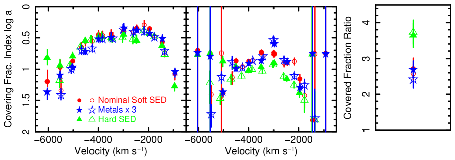
Figure 4: The partial covering parameter $\log a$ constraints. The left panel shows the results for the full model fit to the HST spectra. The open and solid points show the results from the first and second continuum models, respectively (see the text and Paper I for details). The middle panel shows the results from modeling the long wavelength spectra, fixing all parameters except the eleven covering fraction values at their best-fitting values from the UV-only model. The value of the covering fraction parameter $\log a$ is systematically higher, indicating a lower covering fraction (note that the y-axis goes from larger to smaller values). The right panel shows the ratio of the mean $a$ values obtained by fitting a constant between $-4500$ and $-1500\rm\,km\,s^{-1}$. The ratio of the fractions covered by a given opacity approaches these values as $\tau$ approaches $\tau_{max}$. We see that the UV-continuum-emitting region has a larger covering fraction by a factor 2.5 to 3.75 as $\tau$ approaches $\tau_{max}$.

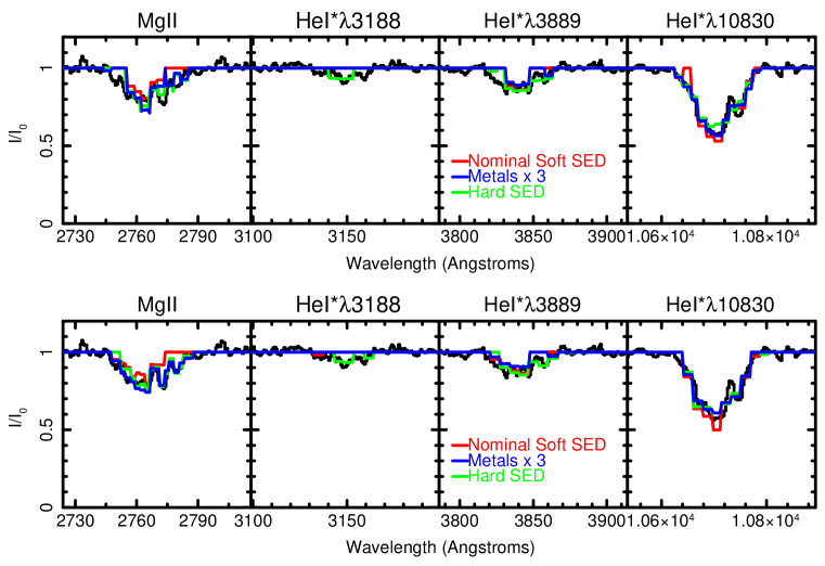
Figure 5: The median spectra for the 11-bin model fit to the optical through near-infrared wavelengths in which the eleven covering fraction values were allowed to vary, but the other parameters (ionization parameter $\log U$, column density parameter $\log N_{H}-\log U$, and density $\log n$) were fixed to the best-fitting values obtained from fitting the HST spectrum (Paper I). The reduced $\chi^{2}$ for these models ranges between 0.66 and 0.84, indicating an acceptable fit, and showing that these three models cannot be distinguished statistically.

While the three different models (the nominal SED, the hard SED, and the metals$\times 3$ case) yield covering fractions in both the UV and at longer wavelengths that follow essentially the same shape as a function of velocity (middle panel in Fig. 4), the normalizations for the different models are slightly different. Specifically, the hard SED model yields a consistently larger covering-fraction index parameter, indicating a lower covering fraction. This is because the hard SED produces a thicker Strömgren sphere (e.g., Casebeer et al., 2006, Fig. 13) and a hotter H II region (e.g., Leighly et al., 2007, Fig. 14), and given that the fraction of neutral helium in the metastable state increases with temperature (Clegg, 1987), more He I* is predicted per metal ion from the hard SED. The near-infrared spectrum has better signal-to-noise ratio than the optical spectrum, and the He I*$\lambda 10830$ is deep compared with He I*$\lambda 3889$ or Mg II, so the He I*$\lambda 10830$ drives the fit. Therefore, it is no surprise that the near-infrared covering fraction obtained from the hard SED simulations is lower than the others. As discussed in Paper I, the hard SED produces the least satisfactory fit to the HST COS spectrum. Therefore, we reject the relatively high covering-fraction ratio derived from the hard SED, and take as the representative value of the ratio of fraction of the UV continuum covered to the fraction of the optical through near-infrared continuum covered to be 2.5.

4.3.1 Spatial Non-Uniformity of the Physical Conditions of the Gas

We have assumed that the only difference between the UV absorption lines and the optical/infrared absorption lines is the covering fraction. But because the infrared continuum emission region is so much larger than the UV continuum emission region (we estimate the area ratios to be $A_{10700}/A_{1100}=140$ in §6.1), it is possible that the physical conditions of the gas are also different. The extrapolation of the UV solution to the optical and infrared absorption lines shown in Fig. 3 reveals the general shape is similar, and therefore the physical conditions are probably not dramatically different. In particular, the “mitten” shape of the He I*$\lambda 10830$ line is reproduced in the extrapolated solution. However, the “thumb” of the mitten, originating in absorption near $\sim-2000\rm\,km\,s^{-1}$ is longer in the extrapolated solution than in the data, suggesting that on average, the outflowing gas with velocity near $-2000\rm\,km\,s^{-1}$ covering the infrared continuum emitting region has somewhat higher opacity than that covering the UV continuum emission region.

We attempted to quantify the possible difference in physical conditions by fitting the optical and infrared $I/I_{0}$ spectrum with a model in which the ionization parameter, $\log N_{H}-\log U$, and covering fraction parameter $\log a$ were allowed to vary. There are no density diagnostic lines in that region of the spectrum, so we froze those parameters at the best fitting values from the UV model. We also froze the velocity offset and velocity width of the bins. Not surprisingly, the results are not very conclusive because there is not enough information among the Mg II and He I* lines to constrain the physical conditions. The ionization parameter is particularly poorly constrained. The $\log N_{H}-\log U$ is consistent with the UV solution within the concentration (between $-4400$ and $-3200\rm\,km\,s^{-1}$). At lower velocities, the $\log N_{H}-\log U$ is higher and the covering fraction parameter $\log a$ is larger (lower covering fraction) in the long wavelength solution compared with the UV solution, but with so few lines to constrain the solution, it is clear that these parameters are highly covariant.

Despite our failure to constrain the physical conditions at long wavelengths, the similarities and differences between the extrapolated UV solution and the observed long wavelength absorption lines suggest intriguing constraints on the spatial uniformity of the absorbing gas.

4.4 What About the Broad-line Region?

We conclude that the absorber in SDSS J0850$+$4451 presents a larger covering fraction to the UV emission region compared with the near-infrared continuum emission region, indicating the presence of structure in the absorbing outflow. Size scales are discussed in detail in §6.1, but it is expected that the broad line region should be located at a comparable or larger radius than the near-infrared-emitting accretion disk. The HST spectrum and continuum models, reproduced from Paper I, are shown for reference in Fig. 6. The rest wavelengths of prominent emission lines are marked. The onset of the outflow is at low enough velocity and the lines are deep enough that is clear that the broad line region is substantially absorbed. Comparison of this figure with Fig. 3 or Fig. 5 shows that the near-UV, optical and near-infrared absorption lines are not as deep as the UV absorption lines (e.g., C IV), giving the impression that the broad line region is fully absorbed, i.e., has a higher covering fraction than the near-infrared continuum emission region, a result that does not make sense considering the relative expected size scales (see §6.1).

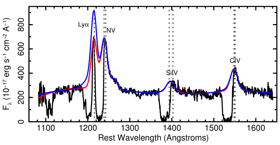
Figure 6: The HST COS spectrum (black line), and continuum models, reproduced from Paper I. The red line shows the first continuum model and the blue line shows the second continuum model; see Paper I for details. The rest wavelengths of prominent emission lines are marked. The onset of the outflow is at low enough velocity, and the lines are deep enough that is clear that at the broad line region emission is absorbed.

This impression is mistaken, due to the nature of the power-law covering fraction parameterization. As discussed in Paper I, in the power-law covering fraction parameterization, the fraction of the source covered, or alternatively, the residual intensity, depends on the total opacity of the line (see also Arav et al., 2005). The prominent UV lines, including C IV, Si IV, and N V, have relatively high opacities, since the ions that produce these lines are very abundant in the H II region of the ionized slab. The ions producing He I*$\lambda 10830$ and He I*$\lambda 3889$, which are also found in the H II region, are rarer, since they come from metastable helium (see Leighly et al., 2011, for a discussion). Mg II is a low-ionization line, and only starts to become commonplace as the hydrogen ionization front is approached (e.g., Fig. 10 in Lucy et al., 2014), so it also has relatively low opacity in SDSS 0850$+$4451 since its LoBAL classification means that the hydrogen ionization front is not present in the outflow (i.e., versus FeLoBALs, where the hydrogen ionization front is expected to be present). Therefore, Mg II is also expected to not be a very optically thick line. Therefore, it is possible that the broad-line region has a lower covering fraction than the UV continuum, even though casual examination of the spectrum suggests otherwise. We discuss inhomogeneous partial covering and the power-law covering fraction parameterization further in §5.

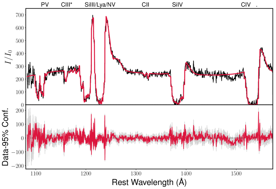
Figure 7: Results from fitting the 11-velocity-bin enhanced-metallicity model to the spectrum between 1080Å and 11500Å; the results for the UV spectrum are shown. In the top panel, the median synthetic spectrum (crimson) is overlaid on the spectrum (black). The lower panel shows the spectrum minus the median model and errors in gray, and the filled region between the spectrum and spectrum and plus and minus the 95% confidence synthetic spectra in crimson, respectively. Comparison with the enhanced metallicity model for the UV spectrum only (Fig. 14 in Paper I) shows that this model yields a comparable-quality fit.

We test this scenario by fitting all of the spectra: the HST COS spectrum analyzed in Paper I that samples the UV band, the combined SDSS and MDM spectra described in §2.4 and §2.5 (sampling the near-UV and optical, between 2500Å and 4000Å), and the combined LBT and Gemini spectra described in §2.1 and §2.2 (sampling the near-IR, between 9000Å and 11500Å). Although we now have developed a method to fit the continuum and line emission simultaneously with the absorption (Leighly et al., in preparation), for direct comparison with Paper I, we separate the line and continuum contributions to our continuum models and fit with the normalizations of these components fixed. As shown in Paper I, there is little dependence on the number of bins used to span the troughs, so the 11-bin model was chosen as representative. Three sets of 11 parameters modeled the covering fractions of the UV, the long wavelengths, and the broad line region, respectively. The UV continuum covering fraction was modeled using $\log a$ as in Paper I. The long wavelength continuum was modeled using $\Delta\log a_{long}$, and a prior was used to constrain these parameters to be greater than zero, i.e., making the physically reasonable assumption that the covering fraction of the longer wavelength continuum is lower than the covering fraction of the UV continuum (as shown in §4.3), and keeping in mind that a larger value of $a$ corresponds to a smaller covering fraction. To be specific, the covering fraction parameter in a particular velocity bin applied to the long wavelength continuum was $\log a+\Delta\log a_{long}$, where $\log a$ is the value applied to the same velocity bin in the UV, and $\Delta\log a_{long}$ is the model parameter. Finally, the broad lines were modeled with an additional $\Delta\log a_{lines}$, thereby making the physically reasonable assumption that the fraction covered is at least as small as that of the long wavelength continuum. Thus, the covering fraction applied to the line emission was $\log a+\Delta\log a_{long}+\Delta\log a_{lines}$.

Overall, the fits are good despite the increase in bandpass. The reduced $\chi^{2}$ computed over the points where the median model experienced opacity (see Paper I; this modified $\chi^{2}$ is used because the continuum is not allowed to vary) are found to be, for the first and second continuum models, respectively: 1.41 and 1.59 for solar metallicity and soft SED, 1.55 and 1.54 for the hard SED, and 1.15 and 1.18 for the soft SED and $\times 3$ metallicity. The values for the solar metallicity and hard SED are larger than the ones obtained for the UV-only models of Paper I (see Leighly et al., 2018, Fig. 5), but are comparable for the enhanced metallicity model, indicating that the $\times 3$ metallicity and soft SED model is preferred. Despite the additional constraints imposed by the inclusion of the long-wavelength spectra, the fit in the UV band is still good (Fig. 7).

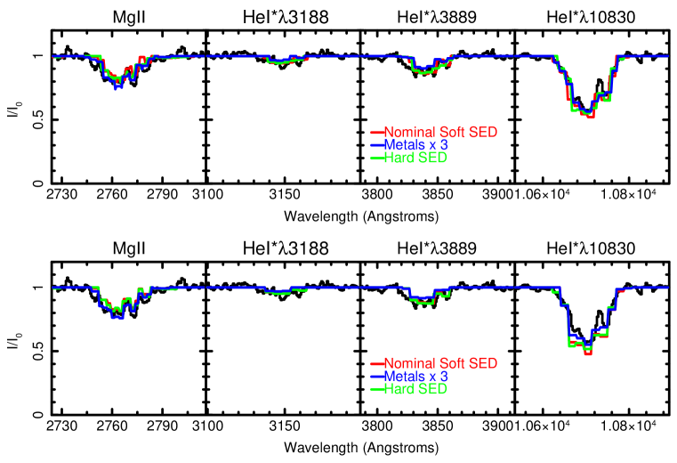
Figure 8: The long wavelength results from fitting the 11-velocity-bin model to the spectra between 1080Å and 11500Å. The models have been divided by the continuum to facilitate comparison with Fig. 5. Overall, the fits are comparable, with minor differences from line to line. We conclude that the model for the full wavelength range provides an excellent description of the spectra.

Fig. 8 shows the results in near-UV to near-IR spectra. Here, the spectra have been normalized by the continuum model to facilitate comparison with extrapolation analysis presented in §4.3. Comparison with Fig. 5 show that the fits are good and overall very similar to one another, although small differences are found from line to line. We conclude that the model presented in this section describes the full bandpass well.

The covering fraction results are shown in Fig. 9. The left-most panel shows the results for fitting the UV continuum and lines together from Paper I. The results from the new model presented in this paper are shown in the right three panels. The second-from-the-left panel shows the covering fraction for the UV continuum alone. The covering fraction index is somewhat smaller than the Paper I result, indicating a somewhat larger covering fraction for the UV continuum than found in Paper I. This is especially true around $-2000\rm\,km\,s^{-1}$, where the line emission is prominent.

The second-from-the-right panel shows the $\Delta\log a$ for the near-UV, optical, and near-IR wavelengths. The difference is particularly strong and robust near $-4000\rm\,km\,s^{-1}$, the location of the enhanced region of $\log N_{H}-\log U$ referred to in Paper I as “the concentration”. This result makes sense, since the ions that produce the long-wavelength lines are found deeper in the photoionized slab and are therefore most prominent in the velocities defined by the concentration. They are also coincident with the C III*$\lambda 1175$ feature discussed in Paper I, e.g., Fig. 6. The $\Delta\log a$ value is close to 0.4, the value obtained in §4.3.

The right-hand panel shows the $\Delta\log a_{lines}$ for the emission-line spectrum. These are, for the most part, consistent with $\Delta\log a_{lines}$ equal to zero. This can be interpreted as evidence that the broad line emission has the same covering fraction as the long wavelength continuum emission region. However, we note that in this model each velocity bin is fit by 3 covering fraction parameters. It seems reasonable to suspect that the data are over-fit, i.e., there are potentially too many covering-fraction degrees of freedom in each velocity bin, resulting in covariance among model parameters.

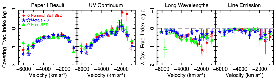
Figure 9: Results from fitting the 11-velocity-bin models to the UV through near-IR spectra. The open and solid symbols correspond the first and second UV continuum models shown in Fig. 6. Points at the end of an error bar denote upper limits. The left-most panel shows the results from Paper I, where the HST spectrum was modeled with a single set of covering-fraction parameters. The right three panels show the results from the model presented in this paper, where the UV continuum was assumed to have the largest covering fraction (corresponding to a lower value of $\log a$), the near-UV through near-IR continuum was assumed to have an equal or lower covering fraction, parameterized by $\Delta\log a_{long}$ required to be greater than or equal to zero, and the emission line region was parameterized by $\Delta\log a_{lines}$, also required to be greater than zero. The results show an offset for the long-wavelength continuum of $\Delta\log a_{long}$ close to 0.4, consistent with the value derived in §4.3. The results for the broad line region show that $\Delta\log a_{lines}$ is essentially consistent with zero, indicating that there is no evidence that the broad line region has a lower covering fraction than the long-wavelength continuum.

Allowing the covering fractions for the UV continuum, the long wavelength continuum, and the broad-line region continuum to vary independently causes the solution to shift compared with the UV-only models presented in Paper I. We find that these shifts are minor and the physical parameters describing the outflow are nearly the same. Fig. 10 shows the outflowing-gas physical parameters as a function of velocity; the results for the UV-only model fits from Paper I are reproduced for comparison. The results for the fitted ionization parameter $\log U$, the column density parameter $\log N_{H}-\log U$, and the derived parameter $\log N_{H}$ are roughly consistent between the two models, with small changes at low velocities where the broad emission lines dominate. The density $\log n$ appears to be much different for velocities higher and lower than that of the concentration (centered near $-4000\rm\,km\,s^{-1}$), but as discussed in Paper I, there are no density-dependent lines at those velocities and the density is unconstrained.

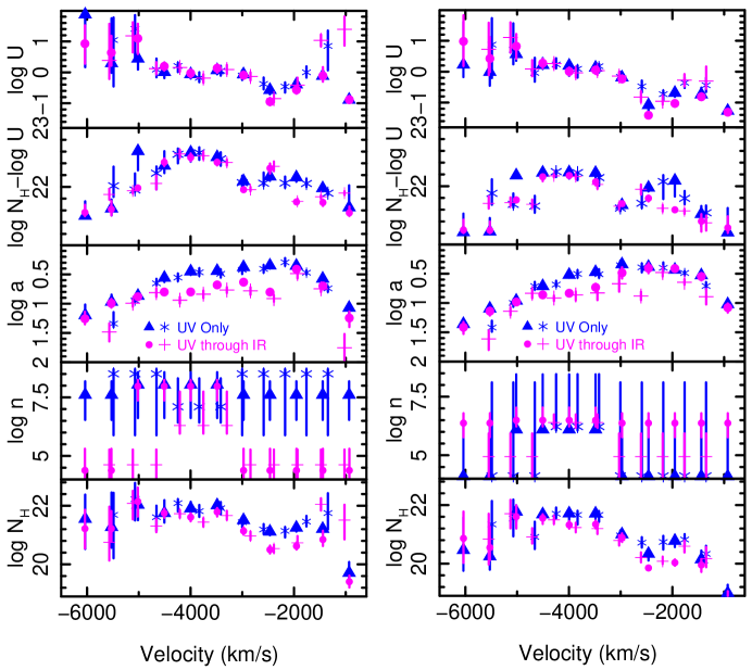
Figure 10: Results from fitting the 11-velocity-bin models to the spectra. The median values and 95% confidence regions from the posterior probability distributions are shown. The left (right) panel shows the results for solar ($Z=3Z_{\odot}$) metallicities, respectively. The star and plus markers (triangle and filled-circle markers) show the results for the first (second) UV continuum models, respectively. The blue symbols show the results from Paper I obtained from modeling the UV spectrum with a single set of covering fractions. The magenta symbols show the results presented in this paper, from fitting the UV through near-IR spectra with three covering fractions. Note that the density $\log n$ is constrained by the presence of C III*$\lambda 1175$ only in the concentration, i.e, between $-4500$ and $-3000\rm\,km\,s^{-1}$ (see Paper I for details. Overall, no significant shifts in the solutions are observed, with the exception of the covering fraction, and the covering-fraction-weighted column density.

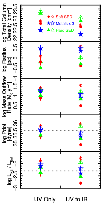
Figure 11: The derived quantities for the 11-velocity-bin model for the UV spectrum only (left side), and from the new analysis of the UV through near-infrared spectra presented in this paper (right side). In each case, the open (filled) symbols show the results using the first (second) continuum model. The top panel shows the total hydrogen column density in the outflow, weighted by the covering fraction in each bin. The column densitiess are lower for the UV through near-infrared models because the covering fraction is lower for larger size scales. The second-from-the-top panel shows the radius of the outflow obtained using the density constraints in the concentration. The next panel shows the mass outflow rate, assuming that the radius of all outflow components is the same as the radius of the concentration. The fourth panel shows the momentum flux $\dot{P}$, applying the same radius assumption, while the dashed line shows $L_{bol}/c$. Finally, the bottom panel shows the ratio of the kinetic luminosity to the bolometric luminosity, again with the same radius assumption. See text for further details. In each case, the median and 1 sigma error bars obtained from the MCMC model are plotted. The UV–near-IR modeling reported in this paper finds a weaker outflow than the UV-only modeling, principally due to the lower covering fraction observed on larger size scales.

Finally, we show the results of the derived parameters including the total column density, the radius of the outflow, the mass outflow rate, the momentum flux, and the ratio of kinetic to bolometric luminosity in Fig. 11. For comparison, we show the results from Paper I as well. In §6.1 we show that the infrared continuum emission region is 140 times larger than the UV continuum emission region. Therefore, the appropriate covering fraction to use for the UV–to–near-IR model is the one for the largest size scale, i.e., $\log a_{long}$ or $\log a_{lines}$, since the properties relevant for the larger area should dominate the outflow, at least as far as we can tell from the information we have. Therefore, we use $\log a_{lines}$ to weight the column densities, resulting in a reduction in the estimated total column density for the enhanced-metallicity models by a factor of $\sim 1.6$ compared with the results of Paper I to $\log N_{H}=22.19^{+0.058}_{-0.056}$ and $22.18^{+0.045}_{-0.043}\rm\,[cm^{-2}]$ for the first and second continuum models respectively (1-sigma errors). The factor of 1.6 is lower than than the ratio of the two covering fractions which was estimated in §4.3 to be 2.5. The difference is that the value of 2.5 was extracted from the well-sampled data in the center of the velocity profile, from $-4500$ to $-1500\rm\,km\,s^{-1}$, while the column density was obtained from the whole profile. If we extract the column density from those that range of velocities only, the difference is a factor of 2.5, as expected.

Other parameters shift due to the reduction in column density and small shifts in the best fit. Specifically, the radius of the outflow is found to be $\log R=0.47^{+0.03}_{-0.04}$ and $0.34\pm 0.04\rm\,[pc]$, the mass outflow rate is $\log\dot{M}=1.07\pm 0.07$ and $0.88^{+0.05}_{-0.06}\rm\,[M_{\odot}\,yr^{-1}]$, and the log of the ratio of the kinetic to bolometric luminosity is $-2.20\pm 0.09$ and $-2.41\pm 0.07$, for the first and second continuum enhanced-metallicity models, respectively. Notably, the kinetic luminosity for the enhanced metallicity models decreases to 0.39–0.63% for the second and first continuum models. This range straddles the 0.5% value taken to be a conservative cutoff for effective galaxy feedback (Hopkins & Elvis, 2010). Therefore, SDSS J0850$+$4451 does not appear to be undergoing strong feedback from the BAL outflow.

To summarize, we have shown that there exists in SDSS J0850$+$4451 a hierarchy of partial covering. The spectra are consistent with a model in which the covering fraction parameter $\log a$ to the optical and near-IR continuum is about 0.4 higher than to the UV continuum (i.e., consistent with the analysis presented in §5, and implying a covering fraction that is lower by a factor of about 2.5). The covering fraction to the broad line region is mostly consistent with that of the long-wavelength continuum, and therefore the broad line region has a lower covering fraction than the UV continuum. In addition, while in Paper I we found only mild support for the preference for high metallicity, the support is much stronger here, given that the reduced $\chi^{2}$ values evaluated over the non-zero opacity portions of the spectra are larger than 1.2 for the solar metallicity and hard SED models, and only the models with $Z=3Z_{\odot}$ are acceptable. Finally, taking into account the lower covering fraction over the larger area results in a reduction in the total column density and other outflow parameters including the kinetic luminosity.

5 Understanding the Power-law Partial Covering Parameterization of Inhomogeneous Partial Covering

The traditional form of partial covering, wherein a fraction of the emission region is covered uniformly by the absorber and the remainder is not covered, is easy to understand intuitively: one needs to only imagine an eclipse. Inhomogeneous partial covering is much less intuitive. Because partial covering seems to be extremely important in shaping the spectrum of SDSS 0850$+$4451, as well as other objects modeled using SimBAL, we explore the nature of partial covering in this section.

Four factors must be considered in order to understand how absorption lines are shaped: the concept of inhomogeneous partial covering itself, the mapping of the output of the photoionization models (ionic column densities) to the power-law parameterization, the opacity of the particular line, and the relative brightness of the background source. We will explore each of these in turn. Note that substantial previous discussions of inhomogeneous partial covering are given in de Kool et al. (2002); Arav et al. (2005); Sabra & Hamann (2005).

5.1 Inhomogeneous Partial Covering and the Power Law Parameterization

The concept of inhomogeneous partial covering can be illustrated using a toy model (e.g., de Kool et al., 2002). Fig. 12 shows linear gray-scale images for two examples of distributions of “clouds”. Each cloud was constructed with opacity in the center of the two-dimensional cloud projection set to $\tau_{0}=1$. The left image illustrates the case where there are many clouds (500) and each cloud has a steep radial opacity profile ($r^{-1.5}$). The right image illustrates the case where there are fewer clouds (150) and each cloud has a flat opacity profile ($r^{-0.5}$). The distribution of optical depths is given in the right panel. As might be expected, many clouds with a steep opacity profile yield low opacity across a large fraction of the continuum source, and a small fraction of the continuum is covered by a high opacity. In contrast, few clouds with flat opacity profiles yield significant opacity across a large fraction of the continuum source.

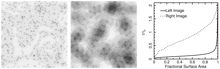
Figure 12: A toy model illustrates inhomogeneous partial covering (see also de Kool et al., 2002). The left images illustrate two scenarios of opacity profile and density of “clouds”, with the far left (middle) image illustrating the case of many (few) clouds with steep (shallow) opacity profiles. The gray-scale is linear, and in each case, the opacity in the center of each cloud, $\tau_{0}$, is equal to 1. The right plot shows the resulting optical depth distribution over the whole image, normalized by $\tau_{0}$. The power law parameterization for inhomogeneous partial covering is intended to model a wide range of distributions of optical depth across a continuum source.

The toy model is useful for illustrating the concept of partial covering, but given that we do not know anything about the “clouds” except their approximate size (§6.2), we use a power-law parameterization for fitting. The power law parameterization is given by $\tau=\tau_{max}x^{a}$ where $x$ is the fractional surface area, as above, and $a$ is the fit index. Fig. 13 illustrates the opacity for different values of $a$. A small value of $a$ corresponds to relatively high opacity over a large fraction of the continuum emission region. A large value of $a$ corresponds to a low opacity over most of the continuum emission region, and a high opacity over a small fraction.

5.1.1 Cloudy and the Power Law Parameterization

As discussed by Sabra & Hamann (2005), the power-law opacity profile $\tau(x)=\tau_{max}x^{a}$ yields the following residual intensity equation:

$$I(\lambda)=\frac{1}{a}\frac{1}{\tau_{max}^{1/a}}\Gamma(1/a)P(1/a,\tau_{max}),$$

where $\Gamma$ and $P$ are the complete and incomplete Gamma functions, respectively. This is the equation that is used in SimBAL.

Cloudy computes photoionization equilibrium in a slab of gas; there is no provision in the software for partial covering. How the ionic column densities produced by the Cloudy simulations map to the power-law opacity profile is a matter of interpretation. There are at least two possibilities: the opacity of an ion calculated using Cloudy corresponds to the average opacity across the continuum emission region (i.e., $N_{ion}\Rightarrow\bar{\tau}$, where $\bar{\tau}=\int_{0}^{1}\tau_{max}x^{a}dx=\tau_{max}/(1+a)$), or the opacity of the ion maps to the maximum opacity (i.e., $N_{ion}\Rightarrow\tau_{max}$). These two methods produce indistinguishable results when the covering fraction is high ($a$ is low), but lead to somewhat different interpretations of partial covering, somewhat different implementations in SimBAL, and different line profile behaviors, as we discuss below.

For the $N_{ion}\Rightarrow\bar{\tau}$ case, we must first obtain $\tau_{max}$ using $\tau_{max}=\bar{\tau}(1+a)$. Thus, the opacity of an ion computed by Cloudy is multiplied by $1+a$ before the spectrum is computed in SimBAL. For the $N_{ion}\Rightarrow\tau_{max}$ case, the opacity computed by Cloudy is used directly as $\tau_{max}$ by SimBAL to compute the spectrum, and the fitted column density is then corrected for the portion that is not covered by dividing by $1+a$ after the SimBAL computation (referred to as the covering-fraction-weighted column density here and in Paper I). There is no difference when $a$ is small, simply because $\bar{\tau}$ approaches $\tau_{max}$. But when $a$ is large, $\bar{\tau}$ is much less than $\tau_{max}$. This fact is illustrated in Fig. 13, where the run of opacity as a function of fractional surface area is shown by the solid lines for a range of $a$ values, and the average opacity is shown by the dashed lines. For large values of $a$, the average value is much less than the maximum value.

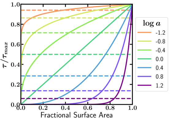
Figure 13: The effects of power-law optical depth parameterization as a function of fractional surface area. The solid lines show the normalized power-law opacity $\tau/\tau_{max}=x^{a}$ for a range of values of $\log a$ shown in the legend. The dashed lines show the average opacity for each value of $\log a$. For large values of $a$, $\tau_{max}$ and the average opacity diverge. $\log a=0.4$ is a value typical of the UV continuum at $-4000\rm\,km\,s^{-1}$ (i.e., in the concentration), and $\log a=0.8$ is a value typical of the wing of the emission lines at $-2000\rm\,km\,s^{-1}$.

If the proportions of ions were uniform as a function of column density of the Cloudy slab, it might seem that there would be no difference between the two interpretations: either the average opacity is scaled up by $1+a$ before the spectrum is constructed, or the inferred column density is corrected by dividing by $1+a$ after the spectrum is constructed. The proportionally of the ionic populations is the assumption that is implicitly made by the $N_{ion}\Rightarrow\bar{\tau}$ method, since it assumes that the optically thickest part of the inhomogeneous partial covering is adequately modeled by $\tau_{max}=(1+a)\bar{\tau}$. However, it is readily apparent that the ionic column densities do not increase in proportion with the hydrogen column density (e.g., Hamann et al., 2002, their Fig. 1). As ionizing photons are removed from the photoionizing continuum by transmission through the gas, the proportions of different types of ions change. This is especially true when approaching the hydrogen ionization front where low-ionization ions such as Mg⁺ start to become common. These low-ionization lines can be very important in constraining the column density. Indeed, in SDSS J0850$+$4451, it is the C III* that constrains the $\log N_{H}-\log U$ of the simulation (see Fig. 10 in Leighly et al., 2018, in particular, see the accompanying animation). For large $a$, it is more important to model the ionic proportions in the high-column density centers of the “clouds,” which is done by the $N_{ion}\Rightarrow\tau_{max}$ method, but not the $N_{ion}\Rightarrow\bar{\tau}$ method.

Further tests show subtle but significant differences in behavior that lead us to reject the $N_{ion}\Rightarrow\bar{\tau}$ interpretation. We created a mock line list to test the differences between the two methods. The mock line list includes a strong line, a weak line, and a blend of four weak lines (Fig. 14). The weak lines all have the same line strength (i.e., same $\lambda f_{ik}N_{ion}$), and the strong line is a factor 20 times larger. Thus, the total opacity of the blend is 5 times smaller than that of the strong line. The left panel shows the synthetic line profiles for a range of $\log a$ values for the $N_{ion}\Rightarrow\bar{\tau}$ method (top panel) and the $N_{ion}\Rightarrow\tau_{max}$ method (bottom panel). The right panel shows the depth of each feature as a function of $\log a$. As expected, the depths of all features decrease with the increase of $\log a$. The difference is seen in the relative decrease of the features for the two methods. For the $N_{ion}\Rightarrow\tau_{max}$ method, the depths of the lines decrease together, maintaining the order of the total opacity. That is, the strong line is always deeper than the blend, which is always deeper than the weak line. This makes sense, because the total opacity of the strong line is 5 times that of the blend, which is in turn 4 times that of the weak line. However, for the $N_{ion}\Rightarrow\bar{\tau}$ case and $\log a>0.7$, the depth of the blend is larger than the depth of the strong line. This is unphysical, since the total opacity of the blend is smaller than the opacity of the strong line. This result occurs because, as mentioned above, in this method, opacities from Cloudy are multiplied by $1+a$ to obtain $\tau_{max}$ before the spectrum is made, and the $1+a$ factor dominates over the actual opacity of the lines for sufficiently high $a$. The same result is obtained if line equivalent width is measured instead of line depth. This problem is most noticeable when modeling overlapping-trough FeLoBALs, where a large $\log a$ means that blends of iron multiplets that are predicted to have low opacity still produce significant optical depth due to the dominance of the $1+a$ factor.

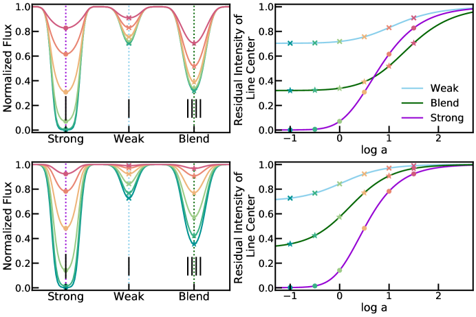
Figure 14: The influence of the choice of mapping of Cloudy output results to the power law partial covering parameters. The top panel shows the results for $N_{ion}\Rightarrow\bar{\tau}$ method, and the lower panel shows the $N_{ion}\Rightarrow\tau_{max}$ method, the method currently used in SimBAL. Left: A strong, a weak, and a blend of four weak lines were simulated for a range of covering fraction parameters $\log a$, where the total opacity of the strong line is 20 times that of the weak line. Right: the depth at the lowest point for the simulated lines shown in the left panel. For the $N_{ion}\Rightarrow\tau_{max}$ case (lower panel), the line depth tracks the total opacity. That is, as $\log a$ is increased (covering fraction decreased), all lines become shallower, but the blended line is always shallower than the strong line. For the $N_{ion}\Rightarrow\tau_{max}$ case (upper panel), the blended line is deeper than the strong line for $\log a>0.7$, even though the total opacity for the blend is five times smaller than for the strong line. This is unphysical, and therefore we reject the $N_{ion}\Rightarrow\bar{\tau}$ mapping.

SimBAL uses the second method, i.e., $N_{ion}\Rightarrow\tau_{max}$. We have run a few tests using $N_{ion}\Rightarrow\bar{\tau}$ on SDSS J0850$+$4451, and we obtain commensurate total column densities (so the derived parameters do not change significantly), but slightly lower log likelihoods (worse fits). This preference for the $N_{ion}\Rightarrow\tau_{max}$ method makes sense for SDSS J0850$+$4451, as the high opacity cores of the clouds that yield sufficient opacity in weak lines such as C III* strongly constrain the $\log N_{H}-\log U$ best fit. But given the unphysical results produced by the $N_{ion}\Rightarrow\bar{\tau}$ method for blended lines as discussed above, we see no reason to investigate this method further.

5.2 The Effect of the Total Optical Depth of a Line

In a slab of ionized gas, the column densities of different ions can be dramatically different. The opacity to C IV can be very large, since this ion is abundant and the transition is easily excited. The opacity to other ions can be very low. In the case of P V, the opacity is low because phosphorus has low elemental abundance compared with carbon. Other ions may have low opacity because they are found at the very back of the matter-bounded slab; for example, for SDSS J0850$+$4451, Mg II and C III* fall into this category. Finally, other ions may have low opacity because they have low oscillator strengths. An example of this category is He I*$\lambda 3889$, which has $f_{ik}=0.064$. Many of the lithium-like ions have oscillator strengths that are much higher; e.g., Mg II has $f_{ik}=0.608$ and $0.303$ for its doublet lines.

These different total optical depths combine with inhomogeneous partial covering to yield different effective covering fractions for different ions. Physically, we can interpret the dependence of effective covering fraction on line opacity in the power-law partial covering parameterization if we imagine an inhomogeneous absorber distributed over the emission region, which is resolved from the point of view of the absorber. For this thought experiment, we do not need to specify the physical form of the inhomogeneity. C⁺³ is a very common ion in photoionized gas, and so it is probable that any line of sight through the inhomogeneous absorber would encounter an optically thick column of C IV. Thus the covering fraction to C IV would be close to 100%. In contrast, P⁺⁴ is rare in photoionized gas, due to its low abundance, and only a few lines of sight through thicker clumps would encounter sufficient P⁺⁴ to produce significant absorption. So the effective covering fraction of P V would be smaller. The same would hold true for other ions that are rare.

We illustrate this behavior by plotting the opacity $\tau(v)$ as a function of fractional surface area for C IV and P V in Fig. 15. We show the results for the SimBAL fit solutions shown in Fig. 7 for two bins corresponding to offset velocities $-4000\rm\,km\,s^{-1}$ (i.e., in the concentration) and $-2000\rm\,km\,s^{-1}$ (on the flank of the broad emission lines). We plot $\tau(v)$ because the opacity from the Cloudy simulation is distributed evenly across a velocity bin in the tophat opacity model; here we use $\Delta v=511\rm\,km\,s^{-1}$, the value obtained as the best fit. Savage & Sembach (1991) relate $\tau(v)$ to the ionic column density $N_{ion}(v)$ through $\tau(v)=2.654\times 10^{-15}f\lambda N_{ion}(v)$ where $f$ is the oscillator strength of the transition, $\lambda$ is the wavelength of the line in Angstroms, and $N_{ion}(v)$ is in $\rm atoms\,cm^{-2}(km\,s^{-1})^{-1}$. The results are seen in Fig. 15. Arav et al. (2005) suggest that the fraction of the surface area with opacity greater than 0.5 provides a good fiducial number for the effective covered fraction. At $-4000\rm\,km\,s^{-1}$ (solid colored lines), the UV continuum covering fraction is $\log a\sim 0.4$, and the effective covered fraction is 100%. At $-2000\rm\,km\,s^{-1}$ (dashed colored lines), the UV continuum covering fraction parameter is still $\log a\sim 0.4$, but the long wavelength and broad-line-region covering fractions are $\log\sim 0.8$. The figure indicates that at $-2000\rm\,km\,s^{-1}$, effective covering fraction of the emission line region is only about 60%. However, the absorption line appears much deeper in the spectrum because the continuum is effectively completely covered, and the wing of the line makes up only 25% of the total flux at $-2000\rm\,km\,s^{-1}$.

Figure 15: The power-law optical depth parameterization convolved with the line optical depth yields the effective covering fraction of the line. Left panel: The opacity of C IV as a function of velocity at $-4000\rm\,km\,s^{-1}$ and $-2000\rm\,km\,s^{-1}$ (solid and dashed lines respectively). The solid gray line shows $\tau(v)=0.5$, a value proposed by Arav et al. (2005) to be characteristic of the effective covering fraction (see text for details). Right panel: The same for P V. $\log a=0.4$ is a value typical of the UV continuum at $-4000\rm\,km\,s^{-1}$ (i.e., in the concentration), and $\log a=0.8$ is a value typical of wing of the emission lines at $-2000\rm\,km\,s^{-1}$. These plots show that for the same covering fraction parameter $\log a$, the effective covering fraction is much greater for C IV than for P V because the total optical depth is much higher.

The right panel of Fig. 15 shows the results for P V. Because $P^{+4}$ is a rare ion, the opacity for P V smaller than that of C IV. At $-4000\rm\,km\,s^{-1}$, the effective covering fraction is about 80%; P V is a shallower line than C IV. The same would be true for other rare ions. At $-2000\rm\,km\,s^{-1}$, the opacity is lower than the fiducial minimum, and no line is observed. This is expected; the solution found by SimBAL yields a lower $\log N_{H}-\log U$ at $-2000\rm\,km\,s^{-1}$ compared with $-4000\rm\,km\,s^{-1}$; the gas is not optically thick enough to produce significant P V. So the P V line is observed to be narrower than the C IV line.

Finally, we display the effective covering fractions for several lines in Fig. 16. In this figure we used the MCMC results and computed the effective covering fraction for each of five absorption lines using the $\tau=0.5$ criterion proposed by Arav et al. (2005), and the appropriate $\log a$ value: the UV continuum $\log a$ for P V, Si IV, and C IV continuum, the long-wavelength $\log a$ for Mg II and He I*, and the broad-line region $\log a$ for C IV BLR. This plot shows that although the BLR has a higher $\log a$ (lower covering fraction) than the UV continuum or the long wavelengths, the effective covering fraction for the C IV BLR is larger than that of P V, Mg II or He I* due to the much greater opacity of C IV.

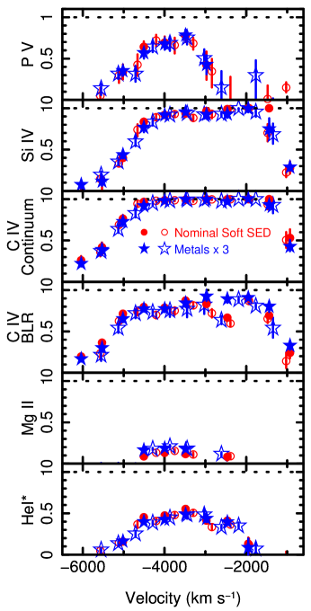
Figure 16: The effective covering fraction as a function of velocity for five lines obtained using the $\tau=0.5$ criterion discussed in the text. For P V, Si IV, C IV, and Mg II, only the results from the stronger doublet line is shown. The open (filled) symbols show the results using the first (second) continuum model. The median values and 95% confidence regions from the posterior probability distributions are shown. The UV continuum $\log a$ was used for P V, Si IV, and the C IV continuum, the long-wavelength $\log a$ was used for Mg II and He I*, and the broad-line region $\log a$ was used for C IV BLR. This plot demonstrates that the covering fraction parameter $\log a$ and the line opacity interact to produce the effective covering fraction. For example, although the value of $\log a$ for the BLR is larger than for the UV continuum, the greater opacity of C IV compared with P V means that the effective covering fraction of C IV BLR is larger than for P V.

5.3 The Effect of the Brightness of the Background Source

The rest-UV quasar spectrum is composed of the continuum emission, presumably from an accretion disk, and emission lines. Depending on the object, most of the lines have moderate equivalent widths, with the exception of Ly$\alpha$, which can be very strong. N V$\lambda 1238$ and Ly$\alpha$ are separated by $\sim 5500\rm\,km\,s^{-1}$, so for outflows with velocities much larger than this value, the N V line will have the Ly$\alpha$ emission lines as well as the accretion disk continuum as a background source. Thus, the N V line can be filled in by Ly$\alpha$, or Ly$\alpha$ can appear as a spike in the N V trough, simply as a consequence of the large intensity of the Ly$\alpha$ line. Different covering fractions for the continuum and emission lines, as might be expected for a relatively compact outflow, also contributes to Ly$\alpha$ leakage. An example of these phenomena is seen in a composite spectrum of strong P V quasars (Capellupo et al., 2017, their Fig. 9). This composite spectrum shows deep absorption in C IV, Si IV, Ly$\alpha$, P V, and O VI, but the N V absorption is quite shallow. Taken at face value, this result might suggest that the absorber is characterized by low ionization, given that N V is a high-ionization line; however, the presence of strong O VI and especially P V, which is known to indicate a high ionization parameter (Leighly et al., 2009) refutes that idea. SimBAL modeling of individual objects explicitly demonstrates that the N V absorption line can be diluted by a strong Ly$\alpha$ emission line (Leighly et al., 2019, also Hazlett et al. in prep).

In summary, inhomogeneous partial covering, modeled here using the power-law parameterization, produces a range of covering-fraction phenomenology that depends both on the covering fraction parameter, but also on the brightness of the background source, as well as the abundance of the ions which in turn depends on the physical conditions in the gas which are solved for using SimBAL.

6 Discussion

6.1 Size Scales in SDSS J0850$+$4451

We have demonstrated that the fraction of the continuum emission region covered is about 2.5 times smaller in the near-infrared compared with the UV in SDSS J0850$+$4451. We have also found that the fraction of the broad line region covered is consistent with the fraction of the near-infrared continuum emission region covered. To understand the implications of these results on the structure of the broad absorption line outflow, we first examine the size scales of the continuum emission region, the broad line region, and the torus, and compare those with the location of the absorber, established in Paper I to be 1–3 parsecs from the central engine.

We used a simple sum-of-black-bodies accretion disk model (Frank et al., 2002) to estimate the sizes of the continuum emission regions. The black hole mass was shown to be $1.6\times 10^{9}\rm\,M_{\odot}$ in Paper I. The log bolometric luminosity was estimated by Luo et al. (2013) to be $46.1\rm\,[erg\,s^{-1}]$. We assumed a standard accretion efficiency of $\eta=0.1$. Using these values, we estimated an accretion rate of $\dot{M}_{acc}=2.2\rm\,M_{\odot}\,yr^{-1}$. This was reported to be smaller than the outflow rate from the wind by a factor of $\sim 8$ by Leighly et al. (2018), but that value is revised to a factor of $\sim 4$ from the results presented in this paper as a consequence of the lower covering fraction over the larger region (§4.4).

We first estimated the continuum emission region sizes (radii) for four wavelengths: 1100Å and 1600Å (values that span the HST spectrum), 2770Å (corresponding to the Mg II absorption line), and 10700Å (corresponding to the He I* line). We used the Wien displacement law and the $T(R)=3GM$Ṁ$/8\pi R^{3}\sigma$ run of temperature for a sum-of-blackbodies accretion disk to estimate the temperatures at which the Planck function should be a maximum at these wavelengths. These values are 0.0016, 0.0027, 0.0056, and 0.034 pc respectively. We find that the radius increases with wavelength as a powerlaw with an index of $4/3$ as expected for a sum-of-blackbodies accretion disk. Thus, the radius of the continuum emission region absorbed by P V is 21 (441) times smaller than the radius (area) of the continuum emission region absorbed by He I*$\lambda 10830$.

This analysis ignores the fact that blackbodies at other temperatures will contribute to the flux at any given wavelength, and that the emission at a given wavelength in a disk needs to be weighted by the radius (e.g., Fig. 5.7, Frank et al., 2002). Fig. 17 shows the radius-weighted flux density at the four wavelengths. The radius at which the emission is maximum is marked, but since there is considerable emission outside of that radius, we identified the size of the accretion disk at each wavelength to be the radius at which the flux density falls to $1/e$ of the maximum value (i.e., roughly the half-light radius). Those radii are 0.0015, 0.0020, 0.0035, and 0.018 parsecs at 1100, 1600, 2770, and 10700Å respectively. These values are comparable to although smaller than the Wein displacement-estimated values above, with radius increasing with wavelength as a powerlaw with an index of $1.16$. Using the radii defined above, we find that the ratio of the area of the accretion disk emitting substantially at 10700Å to the area emitting 1100Å is 140.

These values do not fully account for the difference in continuum emission as a function of radius, because the radius-weighted flux density falls off faster with radius for shorter wavelengths. For example, the slope of the power law tangent to the $1/e$ point increases from $-2.44$ at 1100Å to $-1.45$ at 10700Å. This means that is there is quite a large region of accretion disk where the near-infrared continuum is emitting strongly but the far-UV continuum emission is negligible, but the same cannot be said of the near-UV (near 2770Å) versus the far-UV ($<1600$Å). So, while we can expect to be able to measure a difference in the covering fractions between 1100Å and 10700Å, there is too much emission overlap between the 1100Å and the 2770Å continuum-emitting regions to be able to detect a difference in covering fraction. Thus, we need the long wavelength absorption from He I*$\lambda 10830$ to do these covering-fraction experiments.

These sizes depend on the black hole mass and accretion rate relative to Eddington. SDSS 0850$+$4415 has perhaps a relatively large black hole mass and relatively low accretion rate compared with the expectation for broad absorption line quasars (e.g., Boroson, 2002); either a lower black hole mass or a large accretion rate relative to Eddington would predict a hotter accretion disk. The dependence of the ratio of the 10700Å emission region area to the 1100Å emission region area is explored in Fig. 17. We find that hotter disks predict a much larger ratio of areas, perhaps implying that a more significant difference in the UV versus He I* covering fractions and/or physical conditions might be expected for smaller black hole masses and higher accretion rates. We return to this point in §6.3.

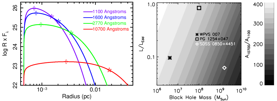
Figure 17: Left: The log of the radius-weighted flux density as a function of radius for the $M_{BH}=1.6\times 10^{9}\rm M_{\odot}$ and $\dot{M}=2.2\rm\,M_{\odot}\,yr^{-1}$ black hole at four wavelengths for the sum-of-blackbodies accretion disk. The location of maximum emission is shown by a diamond, and the star marks the outer radius at which the radius-weighted flux density is $1/e$ times the maximum. Right: The ratio of the area of the accretion disk emitting $10700$Å to the area emitting $1100$Å, where the areas are defined by the radius at which the radius-weighted flux density drops to $1/e$ times the maximum value, and as a function of black hole mass and accretion rate. SDSS 0850$+$4451 has relatively low accretion rate and large black hole mass, yielding a cool disk and relatively small area ratio.

It is interesting to visualize how the accretion disk would appear from the perspective of an observer at the location of the absorber. In Paper I we found that the absorber is constrained to lie in the vicinity of the torus, about 1–3 parsecs from the central engine. At this distance, the 1100Å continuum emission region (diameter) would subtend 3.5–10.5 arcminutes, while the 10700 Å emission would subtend 0.7–2.1 degrees, a bit larger than the full moon.

The size scales and other results computed based on the sum-of-blackbodies accretion disk should be used with some caution, as it can only approximately model the broad-band spectral energy distribution of quasars. It would be interesting to estimate size scales using more sophisticated accretion disk models, such as the one by Done et al. (2012).

In Paper I, we estimated the radius of the H$\beta$ emission to be $0.13^{+0.024}_{-0.021}\rm\,pc$, using the reverberation-mapping regression measured by Bentz et al. (2013). As discussed in Paper I, Luo et al. (2013) fit the H$\beta$ emission-line profile with a relativistic Keplerian disk model, obtaining inner and outer radii of 450 and 4700 $r_{g}$ respectively. For our derived black hole mass, these values correspond to $r_{in}=0.035\rm\,pc$ and $r_{out}=0.37\rm\,pc$ respectively, consistent with the reverberation-mapping estimate. For reference, $r_{in}$ is $10\times$ larger than the $1/e$ radius of the 2770Å emitting region.

We can also estimate the location of the C IV emission region using the regression presented by Lira et al. (2018, Eq. 1). The flux density at 1345 Å is $2.4\times 10^{-15}\rm\,ergs\,s^{-1}\,cm^{-2}$Å^-1, corresponding to $\lambda L_{\lambda}=3.7\times 10^{45}\rm\,erg\,s^{-1}$. The C IV radius is therefore estimated to be $0.028^{+0.039}_{-0.019}\rm\,pc$, where the errors come from the uncertainty on the regression parameters. Using these values, we find that the H$\beta$ emission region is 4.6 times larger than the C IV emission region. This is somewhat larger than but comparable to the values found from reverberation mapping. The Seyferts NGC 5548, NGC 3783, and NGC 7496 show an H$\beta$ lag about 1.8 to 2.8 times the C IV lag (Peterson & Wandel, 1999; Onken & Peterson, 2002; Wanders et al., 1997; Collier et al., 1998). The exception is the double-peaked object 3C 390.3, which showed an inverted relationship, with the C IV lag about twice the H$\beta$ lag.

The size scales for SDSS J0850$+$4451 are shown in Fig. 18 as a function of black hole mass, where we have assumed that the systematic uncertainty in single-epoch black hole mass is 0.43 dex (Vestergaard & Peterson, 2006). Besides the continuum and emission-line radii discussed above, we have also graphed the estimated location of $R_{\tau_{K}}=0.46\rm\,pc$, the hot inner edge of the torus (Kishimoto et al., 2007) computed in Paper I, as well as the estimated radius of the outflow measured in Paper I. The plot shows the expected hierarchy of size scales. Interestingly, the near-infrared continuum emission overlaps the C IV emission region.

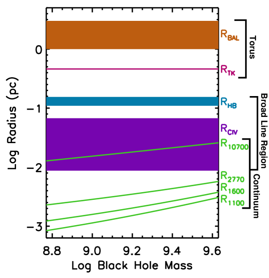
Figure 18: Size scales for SDSS J0850$+$4451 as a function of black hole mass, where the uncertainty in the single-epoch black hole mass estimate is assumed to be 0.43 dex (Vestergaard & Peterson, 2006). From bottom to top, the green lines show the radius at which the radius-weighted flux density drops to $1/e$ of its maximum value (see text for details). The broad line region radii, $R_{H\beta}$ (teal) and $R_{CIV}$ (purple), were computed using the reverberation regressions from Bentz et al. (2013) and Lira et al. (2018), respectively, where the color bands show the uncertainty in the regression parameters. The inner edge of the torus, $R_{\tau_{K}}$ (magenta), was estimated based on the regressions from Kishimoto et al. (2007), while $R_{BAL}$ (orange) is the radius of the broad absorption line outflow measured in Paper I.

6.2 Partial Covering in SDSS J0850+4451

Armed with the quasar size scales, we can discuss the implications of our results on simple scenarios for partial covering in SDSS J0850$+$4451 and BALQs in general.

In one possible scenario for partial covering (left panel of Fig. 20), the size scale of the outflow is large compared with the UV continuum emission region. It would then essentially completely cover the far UV-continuum emission region, but only partially cover the near-IR emission region. This scenario is ruled out because it predicts that covering fraction to the UV continuum would be 100%, and that is not the case.

Alternatively, the absorbing clumps are small, but have internal structure on the size scale of the 1100Å continuum emission region, and the clumps are diffusely distributed on large size scales (middle panel of Fig. 20). In this scenario, similar to the one posited by Hamann et al. (2001, their Fig. 6), each clump might present a distribution of column densities to the continuum source, as would be expected for, e.g., a spherical clump. Each clump would behave as a photoionized slab, with the effective column density and covering fractions of various ions depending on both the abundance of the ion, and where the ion is located within the clump (e.g., on the surface, as might be expected for a high-ionization ion, or buried deep, as expected for a low-ionization ion). Thus, partial covering to the UV continuum is achieved by the structure of the clumps (presenting a range of thicknesses to the illuminating continuum); such a model seems roughly consistent with the power law covering fraction (de Kool et al., 2002). A lower covering fraction to the infrared continuum is achieved by assuming that these clumps are sparsely distributed on larger size scales.

If this scenario is correct, we can estimate the sizes of the individual clumps by dividing the covering-fraction-weighted column density by the density, assuming that the clumps are approximately spherical. There are several additional assumptions that need to be made, however. First, it is probably not reasonable to assume that one clump produces the absorption spanning the whole outflow, i.e., $5000\rm\,km\,s^{-1}$, especially since the covering fraction for a single ion is observed to vary across the trough profile. We assume, somewhat arbitrarily, that a clump spans one velocity bin. We also assume, again somewhat arbitrarily, that velocity bin with the thickest outflow (at $-4000\rm\,km\,s^{-1}$) is most representative. The other bins that have similar covering fraction may be the same size but physically thinner (lower column density and more pancake-like). The bins that have lower covering fractions may have have the same size but a sparser distribution, i.e., a smaller number of clouds across the continuum emission region. This scenario is by no means unique; other configurations could be constructed that are consistent with the analysis results.

The spectra are not very sensitive to the density; this is illustrated by Leighly et al. (2018) in their Figure 11. All we can say with any certainty is that the presence of C III* means that the density is greater than the critical density for that ion, $\log n\sim 10^{6}\rm\,cm^{-3}$. Thus, the cloud size is highly degenerate with density. We illustrate this covariance for the second continuum model and enhanced metallicity run via the corner plot shown in Fig. 19. For that simulation, a typical cloud size (diameter) is $5\times 10^{-4}\rm\,pc=1.5\times 10^{15}\rm\,cm$.

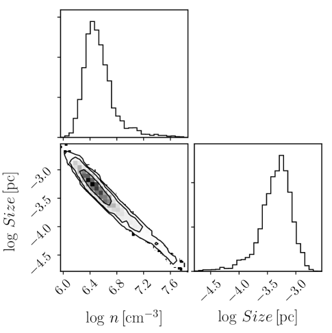
Figure 19: Representative size scales for spherical clouds for the $-4000\rm\,km\,s^{-1}$ velocity bin for the enhanced metallicity and second continuum as a function of density. The contours show the 68, 95, and 99% uncertainty levels. The spectra are generically not as sensitive to density as other parameters. Since the size scale is the covering-fraction-weighted column density divided by the density, the cloud size scale is strongly covariant with the density.

The size scales for the 1100Å and 10700Å continuum emission regions were found in §6.1 to be 0.0015 and $0.018\rm\,pc$, respectively. Assuming that we see the accretion disk face on, and that the inhomogeneous partial covering for the 1100Å continuum emission region is accounted for by weighting the column density with the covering fraction, we find that for the $-4000\rm\,km\,s^{-1}$ bin, approximately 35 clouds are sufficient to cover the emission region. The 10700Å continuum emission region was shown to be 140 times larger, but the covering fraction was found to be 2.5 times lower (§4.3), indicating that $\sim 2000$ clouds would be sufficient to cover the 10700Å emitting accretion disk, if observed face on.

Another possibility is that the clumps are very small, much smaller than the UV continuum emission region (right panel of Fig. 20). In this scenario, the individual clumps should be clustered on size scales smaller than the optical–infrared continuum emission region because if uniformly distributed, identical covering fractions in the UV and long wavelengths would be observed. We note that the difference in distribution is rather modest for this object; in §4.3, we inferred that the UV continuum is a factor of only 2.5 times more densely covered than the optical through near-infrared continuum.

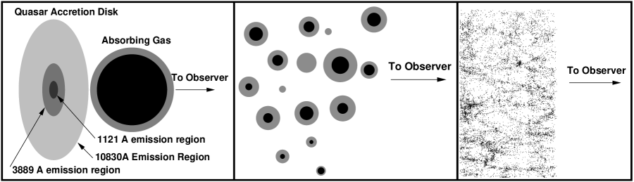
Figure 20: Partial covering scenarios. Left: Geometrical partial covering, in which the absorber only partially covers the emission region (not to scale). Here, the P V absorption line would be expected to fully cover the continuum emission region, while the He I* would show partial covering; this scenario is excluded because the UV continuum is observed to be partially covered. Middle: Inhomogeneous covering, in which the absorber consists of many small clouds that, together, do not completely occult the continuum emission region (adapted from Hamann et al. (2001)). Black represents the higher column density cores of the absorbing clumps, so that C IV absorption (from an abundant ion) will come from the whole cloud (gray + black), while P V and He I* absorption only occurs in the highest column density cores (black). Right: Partial covering characterized by clumping of the inhomogeneous absorbers; the data to create this plot were borrowed from the Two Degree Field Galaxy Redshift Survey (Colless et al., 2001). The clustering of small absorbers predicts both partial covering of UV continuum emission region, and a lower covering fraction for the near-infrared continuum emission region, as we infer for SDSS J0850$+$4451.

Additional information can be obtained from expected time scales of variability. At a distance of 1–3 parsecs from a $1.6\times 10^{9}\rm\,M_{\odot}$ black hole, the Keplerian velocity is between $1500$ and $2600\,\rm km\,s^{-1}$. Considering the 2770Å $1/e$ continuum diameter as a crossing size scale, we find that an orbiting cloud could cross the continuum emitting region in between 2.6 and 4.6 years. This seems to be similar to the time scale of the variability inferred from the Mg II absorption line changes (Appendix A.1), although we note that the pattern of variability perhaps suggests that ionization changes may be responsible (Appendix A.2), rather than covering fraction changes. In contrast, it would take 13–24 years to cross the $1/e$ near-infrared continuum emission region, possibly predicting less variability in the He I*$\lambda 10830$ absorption line.

Finally, while our principal focus has been on the difference in covering fraction between the UV and near-infrared continuum emission regions, we also made measurements of the covering fraction of the broad-line region. We found that there is no strong evidence for a difference in covering fraction between the broad-line region and the long-wavelength-continuum emission region. While it is difficult to know how robust this result is given the large number of degrees of freedom in the models, we note that this result is consistent with the size scales shown in Fig. 18, where the radius of the near-infrared continuum emission region is completely included in the range of C IV emission regions estimated based on the the Lira et al. (2018) regressions.

6.3 Selection Effects and Other Objects

We have demonstrated, using HST COS and optical and near-infrared spectra of SDSS J0850$+$4451, that a difference in covering fraction to the UV and near-infrared continuum emission regions is observed and is quantifiable. We note, however, that this experiment had significant selection effects built in. We chose SDSS J0850$+$4451 for HST COS observations because it showed strong He I* absorption, and because of the similarity in opacity between He I*3889 / He I*10830 and P V predicted over a broad range of physical conditions (Leighly et al., 2011, Fig. 15, Section 4.4.1), we could practically guarantee that P V would be present.

The ratio of the covered portion of the UV continuum-emitting region to the covered portion of the near-infrared continuum-emitting region, was found to be 2.5. In principle, the covered portion of the infrared continuum-emitting region could be much lower. That is, since the $1/e$ radius of the near-infrared continuum emission region (under He I*) is 140 times larger than the radius of the UV continuum emitting region (under P V), objects could exist that have significant P V absorption, but no He I* absorption. In fact, there are two examples where this seems to be the case.

The $z=1.010$ quasar PG 1254$+$047 is known to host P V absorption; it is best known as the original P V quasar (Hamann, 1998). Our LBT observation of this object is described in §2.2. A segment of the PG 1254$+$047 spectrum is shown in Fig. 21, along with the apparent optical depths of the C IV and P V lines, digitized from Hamann (1998) Fig. 3 and shifted to the wavelengths appropriate for He I*$\lambda 10830$ absorption. No evidence for absorption is observed, perhaps implying that the UV absorber does not occult an appreciable amount of the near-infrared-emitting continuum, and indicating a relatively compact absorber. However, the HST observation was made in 1993, and the LBT LUCI observation was made 20 years later, and it is quite possible that the broad-line absorption has changed its properties, becoming optically thin enough that appreciable He I* is not expected, or that the absorber has completely disappeared.

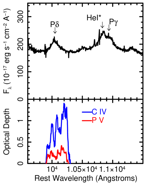
Figure 21: The top panel shows a segment of the LBT LUCI spectrum of the $z=1.010$ quasar PG 1254$+$047. The bottom panel shows the apparent optical depths of the C IV and P IV absorption lines from the HST FOS spectrum (Hamann, 1998) shifted to the wavelengths appropriate for He I*$\lambda 10830$ absorption. No evidence for He I* absorption is seen. This could mean that the absorber does not occult a significant portion of the near-infrared continuum emission region, or that variability in the absorption has occurred between the 1993 HST observation and the 2013 LBT LUCI observation.

Another example is provided by the low-luminosity broad absorption line object WPVS 007. Leighly et al. (2009) reported the emergence of a broad absorption line outflow in the 2003 November 6 FUSE spectrum of this object; a broad P V absorption line was among the lines that were observed. Grupe et al. (2013) presented an near-infrared spectrum obtained in 2004 September 12. Quantitative analysis of the lack of a He I*$\lambda 10830$ line yielded a conservative estimate of the apparent metastable helium log column density of 12.9 [$\rm cm^{-2}$]. In comparison, the apparent log column density of P V in the FUSE spectrum was 15.4 [$\rm cm^{-2}$] (Leighly et al., 2009). The opacity represented as a function of velocity is given by $\lambda f_{ik}N_{ion}(v)$ (Savage & Sembach, 1991), implying that the opacity due to P V at least 41 times the opacity due to He I*$\lambda 10830$, rather than comparable as predicted by photoionization models (Leighly et al., 2011). This result seems to indicate a dramatic difference in the coverage of the UV compared with the near-infrared regions in WPVS 007. However, WPVS 007 is known to have variable absorption lines (Leighly et al., 2009, 2015), leading to some doubt about this robustness of this conclusion. The near-infrared observation was made after the emergence of the broad absorption lines, and broad absorption lines were observed in subsequent HST observations (Leighly et al., 2015) and so it seems unlikely that variability explain the lack of He I* absorption.

A potential interesting difference between WPVS 007 and PG 1254$+$047 versus SDSS 0850$+$4451 is illustrated in Fig. 17. We found that because the black hole masses are smaller in these two objects, their disks are hotter, and the ratio of the area emitting 10700Å to the area emitting 1100Å is larger. The black hole mass and accretion rate for WPVS 007 were estimated by Leighly et al. (2009) to be $M_{BH}=4.1\times 10^{6}\rm\,M_{\odot}$ and $L/L_{Edd}=0.096$. The black hole mass and accretion rate for PG 1254$+$047 were estimated by Sabra & Hamann (2001) to be $M_{BH}=1\times 10^{8}\rm\,M_{\odot}$ and $L/L_{Edd}=0.8$. Using the sum-of-blackbodies disk model described in §6.1 we found that the ratio of the accretion disk area emitting 10700Å to the area emitting 1100Å is 370 and 350 for WPVS 007 and PG 1254$+$047 respectively, much larger than the value of 140 found for SDSS 0850$+$4451. Despite the caveats regarding the sum-of-blackbodies accretion disk model discussed in §6.1, these numbers suggest that it might be reasonable to expect that if outflows are not uniform, then we might be more likely to observe this lack of uniformity in objects with larger area ratios. It is possible that this fact explains the lack of He I*$\lambda 10830$ in WPVS 007 and PG 1254$+$047. On the other hand, both of these objects have smaller black hole masses than SDSS 0850$+$4451, and therefore smaller size scales. If SimBAL analysis of their spectra were to yield a similar solution as for SDSS 0850$-$4451, then the clouds might have similar sizes, and fewer would cover the emission regions. Detailed analysis of more objects would be necessary to deconvolve these effects.

7 Summary and Future Prospects

7.1 Summary of Results

This is the second of two papers investigating the outflow in the low-redshift LoBAL quasar SDSS J0850$+$4451. The first paper described application of the novel spectral synthesis code SimBAL to the HST COS spectrum. We found that the absorber is located about 1–3 parsecs from the central engine, among other results. This paper describes extrapolation of the SimBAL solution to long wavelengths, and the implications for the nature of partial covering in this object. Our principal results follow.

1. In §4.2, we showed that the extrapolation of the best-fitting spectral synthesis model of the UV spectrum of SDSS J0850$+$4451 obtained in Paper I to long wavelengths indicates that the Mg II, He I*$\lambda 3889$, and He I*$\lambda 10830$ lines are all predicted to be significantly deeper than observed, implying that the smaller UV continuum emission region experiences a higher covering fraction than the larger optical / near-infrared continuum emission region.

2. In Appendix A, we discussed the observed variability in the absorption lines, and concluded that the variability is unlikely to have produced the difference in UV and optical/near-infrared covering fractions, but it cannot be ruled out absolutely. In Appendix B we presented analysis of broad-band photometry and an archival HST near-infrared-band image of SDSS J0850$+$4451, and showed that the contribution of the host to the near-infrared continuum is negligible. Therefore, dilution of the He I*$\lambda 10830$ absorption line by the host galaxy continuum cannot be responsible for the difference in UV and optical / near-infrared covering fractions.

3. In §4.3, we found that the absorber covers about 2.5 times more of the far UV continuum emission region than the optical through near-infrared continuum emission region.

4. In §4.4, we performed SimBAL modeling of the UV-through-infrared spectra, using three sets of covering fractions: one for the UV continuum, one for the near-UV through near-infrared continuum, and one for the broad emission lines. We found that the near-UV through near-infrared continuum covering fraction results were consistent with the constrained modeling presented in §4.3, and that the covering fraction of the broad-line region is mostly consistent with the covering fraction of the optical through near-infrared continuum. Considering that the projected size of the infrared continuum emission region is much larger than the UV continuum emission region, we revise the estimated bulk outflow properties from Paper I downward to account for the lower covering fraction. For the statistically-preferred enhanced metallicity model, the estimated column density of the outflow is $\log N_{H}=22.19\rm\,[cm^{-2}]$, the radius of the outflow is $2.2$–$3.0\rm\,pc$, and the mass outflow rate is $\dot{M}=8-12\rm\,M_{\odot}\,yr^{-1}$. Finally, the ratio of the kinetic to bolometric luminosity is 0.4–0.6%. This range straddles the 0.5% value taken to be a conservative cutoff for effective galaxy feedback (Hopkins & Elvis, 2010). Therefore, SDSS J0850$+$4451 does not appear to be undergoing strong feedback from the BAL outflow.

5. In §5, we discussed inhomogeneous partial covering and the power-law parameterization used by SimBAL. Four factors that must be considered in order to understand how absorption lines are shaped: the concept of inhomogeneous partial covering itself, the mapping of the output of the photoionization models (ionic column densities) to the power-law parameterization, the opacity of the particular line, and the relative brightness of the background source. In particular, we show how the observed absorption lines depend on the value of the covering fraction parameter $\log a$ but also on the abundance of the ions. So, a rare ion such as P⁺⁴ can produce a shallower absorption line against the UV continuum than a common ion such as C⁺³ against the broad-line region, even though the covering fraction is lower for the latter.

6. In §6.1 and §6.2, we examined the size scales of the continuum emission region (accretion disk), the broad-line region, the torus, and the outflow (estimated to be 1–3 parsecs in Paper I). To explain the partial covering in the UV (established in Paper I), and the difference in covering fractions between the UV and long wavelengths, we suggest a model in which the outflow consists of clumps that are individually structured or very small relative to the UV continuum emission region size scale, and are themselves clustered on size scales comparable to the near-infrared continuum emission region size scale.

7. In §6.3, we note SDSS J0850$+$4451 was chosen for this experiment based on the previous observation of He I*$\lambda 10830$ absorption, and that in principle, there may be objects which show strong UV absorption but no infrared absorption. We discuss two examples where this seems to be the case, but note that the UV and infrared observations were not simultaneous (and in the case of PG 1254$+$47 were separated by 20 years), so variability cannot be ruled out.

7.2 Conclusions and Future Prospects

In this paper, we show that broad absorption lines widely separated in wavelength can be used to investigate the nature of partial covering. This experiment shows that we need not be limited to knowledge about outflows along the radial light of sight to the continuum emission region, but we can also learn about the angular distribution of the outflowing clumps.

It would be interesting to investigate other objects using this method. The ideal experiment would involve an object known to have P V absorption, so that absorption from He I*$\lambda 10830$ would also be predicted (Leighly et al., 2011). This requires the object to have a redshift of less than $\sim 1.2$ (depending on the velocity of the outflow) so that He I*$\lambda 10830$ can be observed from the ground. The redshift requirement means that UV spectrum would need to be observed using HST. The UV and near-infrared observations should be contemporaneous, in order avoid uncertainty due to variability. Depending on the quasar luminosity, an near-infrared image may be advisable to quantify the host galaxy contribution to the 1-micron continuum.

Appendix A Absorption Line Variability

A.1 Observed Variability

Vivek et al. (2014) presented the results of time variability studies of Mg II and Al II absorption lines in a sample of 22 LoBAL quasars. Their sample included SDSS J0850$+$4451. They obtained several spectra at the IUCAA Girawali Observatory (IGO) in 2010 and 2011. While there was no variability among the 2010 and 2011 observations, there was significant variability when compared with the 2002 SDSS spectrum: the equivalent width of the absorption line increased from $12.6\pm 0.4$Å to (weighted mean) value of $18.9\pm 0.6$Å.

This result spurred us to obtain two additional spectra in April 2014 (APO), and April 2015 (KPNO) to measure the He I*$\lambda 3889$ and Mg II absorption lines. The descriptions of these data sets are given in §2.6 and §2.3. Combined with the MDM spectrum from 2011, a digitized Vivek et al. (2014) spectrum from 2010, and the BOSS spectrum from January 2015, we can examine the absorption line variability observed over 12.5 years (observed frame, 8.1 years rest frame). We focus on the Mg II and He I*$\lambda 3889$ lines, as they are deepest, and model the two regions separately. With the goal of quantifying the absorption variability, we fit all spectra containing each line simultaneously using Sherpa (Freeman et al., 2001). The continuum model is similar to the one described in §3 in most cases. The exception was the 2015 BOSS spectrum which displays an unusual continuum shape at shortest wavelengths. We modeled the continuum of that spectrum with a 3rd order polynomial. The KPNO spectrum, taken three months after the BOSS spectrum, shows a normal AGN continuum, and therefore, we suspect that the BOSS spectrum suffered bad flux calibration. As noted above, this should not be the well-known BOSS spectrograph differential refraction problem (Margala et al., 2016), as that is now corrected for in the pipeline.

For the Mg II region, we tie the widths of the Mg II emission lines together between spectra, and model the absorption with a single Gaussian opacity profile. Our first model left the central wavelength and width of the opacity model independent among the epochs. The reduced $\chi^{2}$ was 0.85 for 7138 degrees of freedom. In order to make the simplest comparison of opacity (the factor we are most interested in), we try a second model with the position and widths tied together. The $\chi^{2}$ was slightly worse (0.87 for 7146 degrees of freedom), but an application of the F-test indicated only 17% chance that the difference was significant.

For the He I*$\lambda 3889$ region, we tie the widths of the [Ne III]$\lambda 3870$ emission lines together among the spectra, and model the He I* absorption line with a single Gaussian opacity profile. In this case, the fits are indistinguishable when the absorption line widths and positions are free or tied together (in both cases, $\chi^{2}_{\nu}=0.96$ for 7156 and 7164 degrees of freedom, respectively).

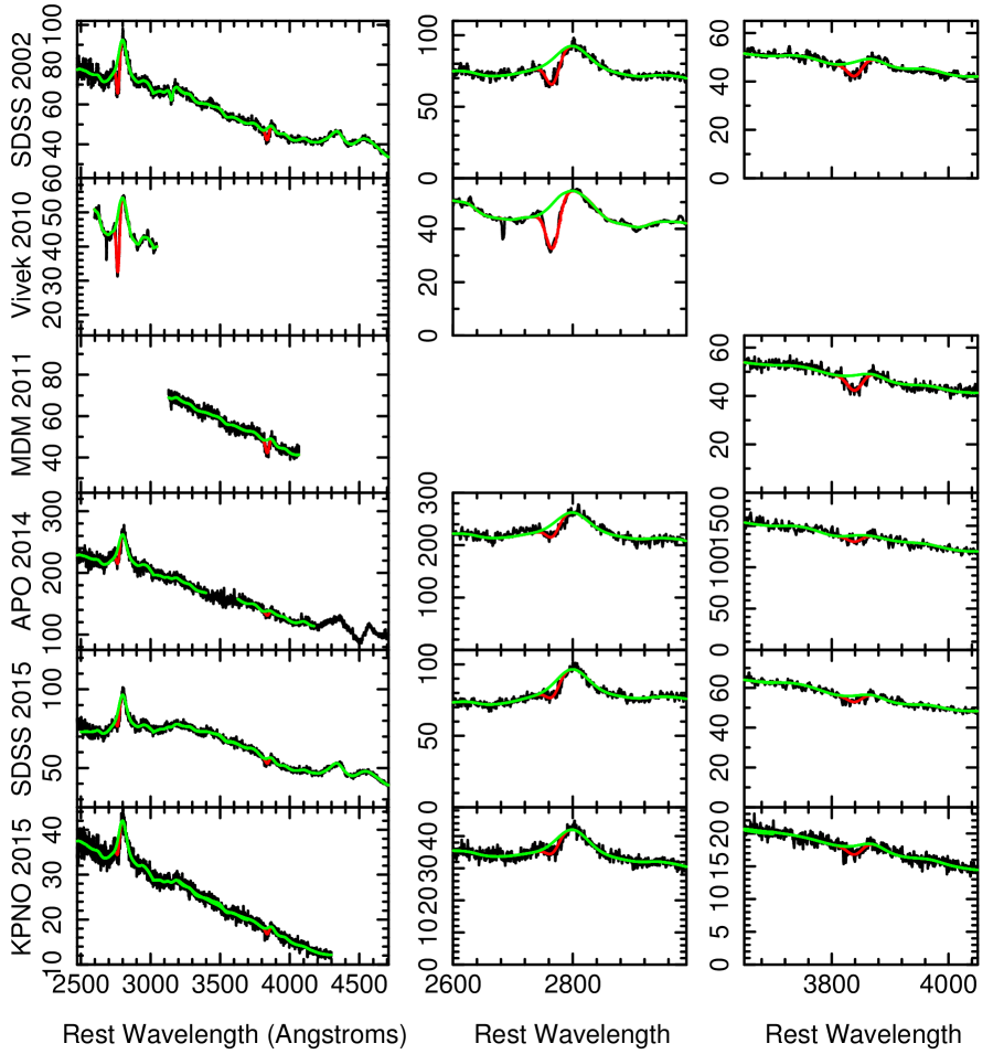
Figure 22: Results of spectral fitting used to extract the opacities of the Mg II and He I*$\lambda 3889$ lines. The spectra are plotted as a function of rest wavelength and flux density $F_{\lambda}\,(10^{-17}\rm\,erg\,s^{-1}\,cm^{-2}$Å${}^{-1})$. The spectrum labeled “Vivek 2010” was digitized from figures shown in Vivek et al. (2014). Note that the “MDM 2011”, “APO 2014”, and “KPNO 2015” spectra are not accurately fluxed. The spectra were fit simultaneously in the Mg II and He I* regions separately. The best fitting model is overlaid in red, while the model without the line absorption is overlaid in green. The variability of the Mg II and He I*$\lambda 3889$ lines is clearly seen.

The resulting fits are shown in Fig. 22. The resulting apparent optical depths for Mg II and He I*$\lambda 3889$ are presented in Fig. 23. Also marked are the dates of the near-IR observations (using LBT LUCI and Gemini GNIRS) and UV observation (HST COS). This plot clearly shows that while the MDM observation of He I*$\lambda 3889$ was contemporaneous with the near-infrared observations using LBT and Gemini, there are unfortunately no ground-based observations within one year of the HST COS observation.

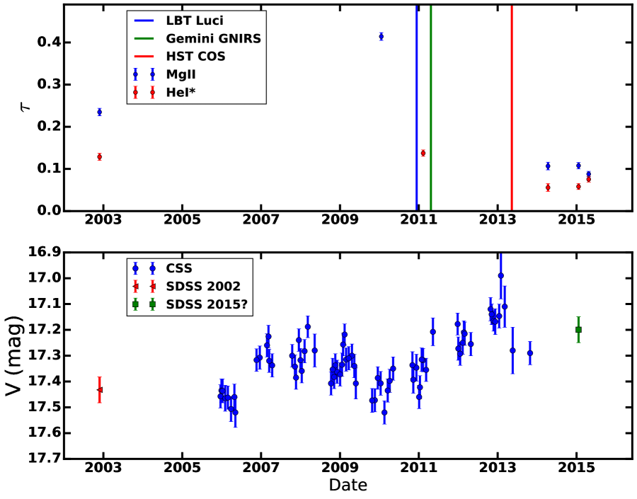
Figure 23: Upper panel: The evolution of the Mg II and He I*$\lambda 3889$ optical depths. The absorption lines were modeled using a Gaussian opacity profile, and the values shown are the normalization. Since the widths and positions were tied together for each species in the spectral fitting, the normalization is proportional to the apparent column density / optical depth. The He I* optical depth varied by a factor of two. The Mg II line varied by a larger factor among the five observations than the He I* line (by a factor of 4), but this result is not conclusive given that we do not have a measurement of He I*$\lambda 3889$ absorption when the Mg II line was strongest. Lower Panel: The v-magnitude variability observed using SDSS and the Catalina Sky Survey. The trends suggest that the absorption lines are shallower when the object is brighter, and were therefore shallow when the HST observation was performed.

After an initial increase in opacity by a factor of 1.8, the Mg II absorption line decreased to a value slightly less than half the value observed in 2002. Thus, the apparent opacity of the Mg II line was observed to vary by a factor of more than four. The He I*$\lambda 3889$ displayed less variability (factor of 2). However, we do not have a measurement of the He I*$\lambda 3889$ line in 2010 when the Mg II was so strong, and when we compare the only the results from observations where both lines were observed, the relative variability is similar. We conclude that the degree of variability is the same for both lines, or larger for Mg II.

We note that the spectra that we took are not accurately fluxed, so we cannot compare the absorption variability with the continuum variability directly. To compare the continuum variability with the opacity, we downloaded the Catalina Sky Survey (CSS) data for this object. The data, shown in Fig. 23, consists of the error-weighted average per night. Vivek et al. (2014) also analyze these data. It is noteworthy that the magnitudes plotted in their Appendix B are about 0.5 magnitude fainter than the data we downloaded. The origin of this difference is not understood. We speculate that the difference originates in an updated calibration of the CSS data to the Johnson V band. We also plot the V-band magnitude from the SDSS observation, obtained using color correction terms from Jester et al. (2005). The uncertainty was taken to be the color transformation RMS residual.

The photometry shows that SDSS J0850$+$4451 is very modestly variable; the standard deviation on the photometry points is 0.11 mag, corresponding to a factor of 10%. However, quasars are known to be bluer when brighter, so a larger degree of variability may be present in the photoionizing continuum.

Comparing the photometry with the opacity, we see that in general the line opacities are inversely related to the flux. More specifically, the V-band flux was relatively low when the Mg II opacity was highest, in 2010, and since then, the V-band magnitude has tended to increase, and the line opacities to decrease. This suggests that at the time of the HST COS observation, the Mg II and He I*$\lambda 3889$ opacities were no higher than observed during the 2002 SDSS observations. This implies that, if anything, the Mg II and He I* lines were shallower the ones in the spectra that we analyze in this paper. Therefore the discrepancy between the extrapolated spectral synthesis models and the observed troughs shown in Fig. 3 would be potentially larger.

In summary, the opacity and flux trends suggest that the differences in partial covering that we measure are not an artifact of variability. However, because we do not have contemporaneous optical and infrared spectra at the time of the HST spectrum, we cannot rule this explanation out absolutely.

A.2 Predicted Variability Patterns

There has been an explosion in variability studies of broad absorption line quasars in recent years (e.g., Capellupo et al., 2011, 2012, 2013; Filiz Ak et al., 2013; Vivek et al., 2014; McGraw et al., 2015, 2018). Such studies can be used to constrain the distance of the absorber from the central engine, and thereby constrain feedback metrics; for an example of such an analysis and additional references, see McGraw et al. (2018). The distance can be constrained if there are changes in covering fraction by assuming that Keplerian motion carries the absorber across the continuum source; McGraw et al. (2018) found typical distances $r\lesssim 1$–10 pc in their sample of P V quasars. If there are changes in ionization parameter, the distance can be constrained by comparing the observed variability time scale with the recombination time scale; McGraw et al. (2018) found a typical range of $r\lesssim 100$–1000 pc.

These variability studies have taken a general, qualitative, and order-of-magnitude approach to the estimation of the origin of BAL variability. SimBAL, in contrast, can place qualitative constraints on the origin of variability. We use the SimBAL simulation grids to predict the kinds of variability that might be observed in Mg II, He I*$\lambda 3889$, and He I*$\lambda 10830$ absorption lines as a function of a change in ionization parameter $\log U$ (equivalent to a change in ionizing flux for a fixed density), a change in the column density $\log N_{H}$, or a change in the covering fraction, parameterized by $\log a$, that might be equivalent to transverse motion across the source.

We chose the 11-bin models from Paper I for the second continuum for the nominal soft SED, the hard SED, and the enhanced metallicity cases. We varied one parameter at a time by the same amount in each of the eleven velocity bins. At each deviation interval away from the best fit, we created a synthetic spectrum, and then estimated the apparent column density of Mg II, He I*$\lambda 3889$, and He I*$\lambda 10830$, by integrating over the line profile, using Eq. 9 in Savage & Sembach (1991). The results are shown in Fig. 24.

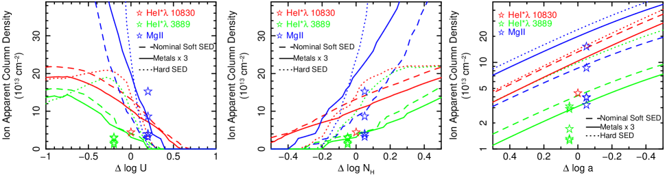
Figure 24: The predicted variation of the apparent column densities of Mg II, He I*$\lambda 3889$, and He I*$\lambda 10830$ as a function of one varied parameter away from the best-fitting solution obtained from the UV spectrum. Also shown as open stars are the apparent column densities measured directly from the spectrum for He I*$\lambda 10830$, and from the model fits, for Mg II and He I*$\lambda 3889$. These are offset along the x-axis for clarity.

An increase in $\log U$ results in a decrease in the opacity for all lines, but especially for Mg II, because the regions in the slab where Mg⁺ and excited-state neutral helium lie are matter bounded. So an increase in the ionization effectively pushes the regions where these ions would be present beyond the back (i.e., opposite of the illuminated face) of the cloud. Increasing the thickness of the clouds causes the opacity for all the lines to increase, but, again, especially for Mg II. The interpretation is the same as above. The column densities for the best fitting model is matter-bounded for these ions, so increasing the total column density increases the column density of these ions. The powerlaw covering fraction model has the property that all opacities increase geometrically. There are slight differences in slope but those are not significant. Finally, it is important to note that in all cases, the He I*$\lambda 10830$ line varies in concert with the He I*$\lambda 3889$ line.

The data are insufficient to determine which of these scenarios (variable ionization parameter, variable column density, or variable covering fraction) is true. But the pattern of variability observed seems to weakly support variation in ionization parameter, since, as discussed in §A.1, there is a possible anti-correlation observed between the opacity and continuum flux, and a greater variability in Mg II compared with He I*$\lambda 3889$. Vivek et al. (2014) suggested that ionization variability might have occurred in SDSS J0850+4451.

Appendix B The Host Galaxy Contribution to the Near-Infrared Continuum

As noted above, the observed He I*$\lambda 10830$ absorption line is much shallower than predicted by the model of the far-UV spectrum. This could mean that the covering fraction to the near-infrared continuum is lower than it is to the ultraviolet continuum. But another possibility is that the host galaxy is contributing a significant amount of the observed near-infrared continuum, making the He I*$\lambda 10830$ line appear shallower than it really is. In this section, we estimate the plausible contribution of the host galaxy to the near-infrared continuum to address this second possibility. We found that the contribution of the host galaxy is negligible.

B.1 SED Fitting

Lucy et al. (2014) addressed the question of the host galaxy contribution to the near-infrared continuum of FBQS J1151$+$3822 via SED modeling of broadband photometry. They fit data from SDSS, 2MASS, and WISE with a power law, elliptical galaxy template, and two blackbodies to model both the warm ($T\approx 1200\ {\rm K}$) torus and cooler ($T\approx 300\ {\rm K}$) dust.

We follow that procedure here, but we use our new $JHK_{s}$ photometry, add NUV photometry from GALEX, and include two ultraviolet continuum points derived from the HST COS spectra (Paper I). The SED is shown as black filled points in the upper panel of Fig. 25, along with the original 2MASS values in red; these were not used in the SED fitting. We first obtained an estimate of the reddening in SDSS J0850$+$4451 by building a simple model consisting only of the Richards et al. (2006) continuum. This model has only two parameters: a multiplicative scaling of the Richards continuum and the reddening intrinsic to the quasar. This model was fit to all points excluding those from WISE, and yielded $E(B-V)=0.03\pm 0.03$. The WISE points were excluded because, compared to the Richards continuum, the torus in SDSS J0850+4451 is considerably less bright, suggesting that this object is deficient in hot dust (Hao et al., 2010, 2011; Lyu et al., 2017).

Also shown in the top panel of Fig. 25 is the decomposition of the SED with components indicated in the figure legend. This solution has reddening $E(B-V)=0.0$, meaning that the solution hit the lower bound of allowed values. The galaxy contribution at $\lambda=10830\ {\rm\AA}$ is $0.09\pm 0.03$%. The power-law index is $-1.53$, which is not unusual for quasars (Krawczyk et al., 2015). The residuals to the fit are shown in the lower panel of the figure, where these are defined as $\Delta=$ (data $-$ model) / model. The model fit is not particularly good, with reduced $\chi^{2}=50$, but much of this is likely to be due to the simplicity of the model; variability may play a role as well (see Fig. 23). These results show that the contribution of the host galaxy emission to the continuum under the He I*$\lambda 10830$ absorption line is negligible.

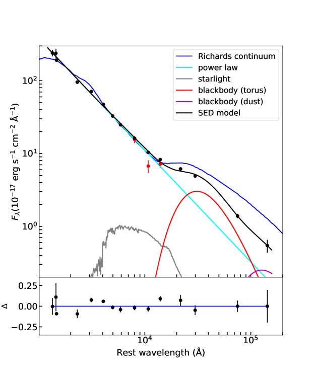
Figure 25: Spectral energy distribution modeling to SDSS, WISE, and observed JHK photometry. The SDSS photometry has been corrected for the contribution of emission lines (Lucy et al., 2014). The blue line shows the Richards et al. (2006) composite quasar spectrum fitted shortward of several microns, and extrapolated to long wavelengths, illustrating the lack of strong near-infrared emission from the torus compared with average quasars. The contribution of the host galaxy to the continuum under negligible, and is consistent with the imaging analysis presented in Fig. 27.

B.2 Image Analysis of the SDSS J0850+4451 Host Galaxy

Coincidentally, an HST program made WFC3 observations in the near-infrared of SDSS J0850+4451; the information about this observation is found in Table 2. We used these data to provide a complementary estimate of the contribution of the host galaxy to the infrared continuum emission and the photometry.

HST images of quasars are dominated by the quasar, so it is necessary to use the image point spread function (PSF) to isolate the emission of the host galaxy. A PSF made from observations of a star works better than a simulated one (e.g., Canalizo et al., 2007), and fortunately, a PSF star observation was made in association with this program. The star was the white dwarf GRW+70D5824, an object chosen to have $B-V$ color similar to the average color of the sample. It was observed with three different exposure times in each filter in order to obtain a broad dynamic range. The star was placed on the same part of the detector as the science observations. HST has variable focus (so-called “breathing”). Fortunately, the star and the quasar were observed during times when the focus was nearly the same. The PSF is undersampled by the detector, but that is accounted for by dithering the telescope during the observation, and combining the individual images using the MultiDrizzle software, which also corrects for distortion.

Cosmic-ray rejection can remove photons from the core of the image (Riess, 2011). To determine whether this problem is present in the multidrizzled images, we performed photometric analysis on the flat-fielded images of the star. We obtained a mean and standard deviation of the net count rates for the star of $1.500\pm 0.009\times 10^{-15}\rm\,erg\,s^{-1}\,cm^{-2}\,$Å^-1. The aperture correction for the F125W filter from 2 arc seconds to infinity is 0.029 (Kalirai et al., 2009), resulting in a final estimated flux density of $1.539\pm 0.009\times 10^{-15}\rm\,erg\,s^{-1}\,cm^{-2}\,$Å^-1. The 2MASS $m_{J}$ is 13.248, corresponding to a flux density of $1.57\times 10^{-15}\rm erg\,s^{-1}\,cm^{-2}\,$Å^-1, less than 2% from the measured value. In contrast, a similar extraction of the multidrizzled images (i.e., after cosmic-ray correction) yields an flux estimate of $1.392\pm 0.006\times 10^{-15}\rm\,erg\,s^{-1}\,cm^{-2}\,$Å^-1, 11% below the 2MASS value, indicating that indeed, cosmic-ray rejection had removed source photons from the core of the image.

We performed roughly the same analysis on the image of SDSS J0850+4451, but since we wished to compare with the MDM photometry, we first blurred the image by convolution with a Gaussian to correspond to the 1.25 arc second seeing. The resulting measurement of the flux density was $8.75\pm 0.18\times 10^{-17}\,\rm erg\,s^{-1}\,cm^{-2}\,$Å^-1. In contrast, the multidrizzled image yields a measurement of the flux density of $6.90\pm 0.12\times 10^{-17}\,\rm erg\,s^{-1}\,cm^{-2}\,$Å^-1, about 20% lower. Nevertheless, this difference should only influence the core of the quasar PSF, and not the extended host galaxy emission.

The image analysis was done using Sherpa (Freeman et al., 2001). This software requires three input images: the target image, an error image, and a point spread function image. The point spread image was constructed using the five observations of the PSF star: three with exposures of 5.865 seconds, one with exposure of 11.729, and one with exposure 23.458 seconds. We examined the images and the data quality arrays and found no evidence for saturation. Therefore, an exposure-weighted average of these images was used for the PSF. We smoothed the PSF image using the method outlined by Canalizo et al. (2007). To prepare the error images, we followed the procedure outlined in The DrizzlePac Handbook.

We modeled a circular region within 71 pixels (9.23 arc seconds), excluding three faint sources near the edges of the region. Initially, we chose a Gaussian model and a constant background. This model did not provide a good fit to the image, with a reduced $\chi^{2}_{\nu}=4.05$. We next tried a model consisting of a Gaussian profile, a Sersic model, and a constant. The resulting reduced $\chi^{2}_{\nu}$ was 1.34, a dramatic improvement in fit over the Gaussian plus constant model that indicates clear evidence for the detection of the host galaxy.

Statistically, the Gaussian plus Sersic model provided a good fit. However, examination of the radial profile showed positive residuals between 2 and 5 arc seconds from the center, suggesting that there is an additional larger-scale but fainter component. We model this component with an additional Sersic profile, but because the error bars are large, we fixed the index to one (appropriate for a disk galaxy) and the ellipticity to zero. The $\chi^{2}$ decreased a small amount, to $\chi^{2}_{\nu}=1.27$, indicating that this component is not statistically necessary. The fit parameters are given in Table 2, and the image, best fitting model, residuals, and profile are shown in Fig. 26.

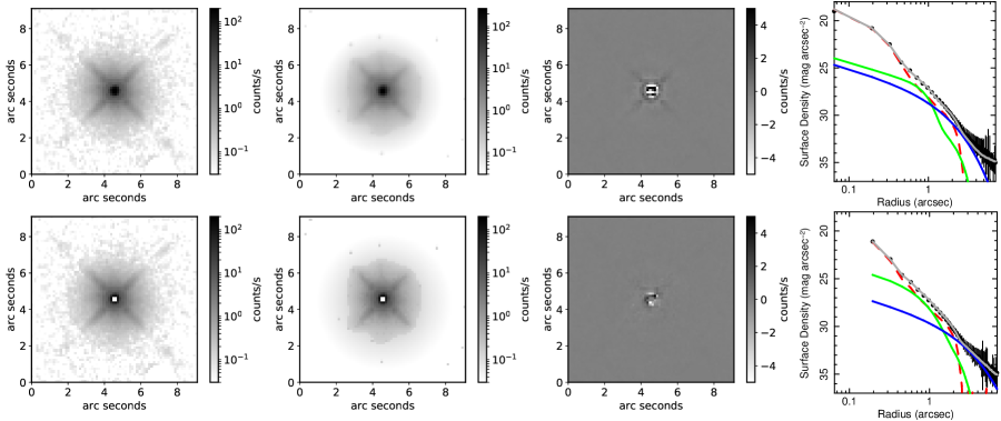
Figure 26: The results of analysis of the HST IR F125W image of SDSS J0850+4451. The model consisted of a two-dimensional Gaussian and two Sersic models. From left to right: the data, the fitted model convolved with the PSF, the difference between the data image and the model, and the radial profile from the data and the model. The top panel shows the results from analysis of the whole image, and the bottom panel shows the results with the central four pixels removed from the fitting. The host galaxy in SDSS J0850+4451 is clearly detected.

Noting the problems with cosmic-ray rejection in the core of the PSF discussed above, we performed the same analysis but ignored the four central pixels. The reduced $\chi^{2}_{\nu}$ for this model was 0.58. The same residuals were observed in the radial profile, so we added another Sersic model as above, producing a reduced $\chi^{2}_{\nu}$ of 0.51. The model parameters are given in Table 2, and fitting results are shown in Fig. 26.

Table 2: Image Fitting Results

Parameter	Full Image	Central 4 Pixels Removed
Gaussian FWHM (pixels)	1.36^+0.006_-0.0.05	0.73^+0.12_-0.002
Gaussian Amplitude (counts s-1)	1332±9	4250^+17_-1100
1 Sersic $R_{0}$ (pixels)	5.0^+0.06_-0.04	4.4^+0.31_-0.04
1 Sersic $R_{0}$ (kpc)	4.1^+0.05_-0.03	3.6^+0.25_-0.03
1 Sersic Eccentricity	0.16^+0.009_-0.008	0.12^+0.02_-0.009
1 Sersic Theta (radians)	0.91±0.02	1.0^+0.04_-0.12
1 Sersic Amplitude (counts s-1)	2.0^+0.05_-0.07	2.5^+0.04_-0.17
1 Sersic $n$	0.21 ±0.02	0.53^+0.01_-0.13
2 Sersic $R_{0}$ (pixel)	9.8^+0.4_-0.5	17^+2_-3
2 Sersic $R_{0}$ (kpc)	7.9^+0.34_-0.40	14^+1.6_-2.6
2 Sersic Amplitude (counts s-1)	0.3^+0.04_-0.03	0.07^+0.06_-0.012
Constant (counts s)-1	0.010^+0.0007_-0.0006	0.006 ±0.001

Sherpa allows us to save the unconvolved model component images. The count rates from each component were obtained by summing over these images, and converted to flux densities using the inverse sensitivity. These values are given in Table 2. We note that the value obtained from the fit with the four central pixels excluded ($8.5\times 10^{-17}\rm\,erg\,s^{-1}\,cm^{-2}\,$Å^-1) is comparable to the value obtained using aperture photometry on the flat-fielded images, as described above ($8.75\times 10^{-17}\rm\,erg\,s^{-1}\,cm^{-2}\,$Å^-1), indicating that our model accounts for the emission in the image. Also, the flux densities from the galaxy component are essentially the same whether we ignore or keep the four central pixels, indicating that the issues stemming from the imperfect cosmic-ray rejection did not affect the estimate of the host galaxy flux.

We convolved the model component images with the seeing and applied an aperture to estimate the flux from each component contributing to our photometry and spectroscopy. We did this for two cases. The first case pertains to the MDM JHK photometry described in §2.4. The seeing during those observations was about 1.25 arc seconds (about 4 pixels) and the extraction aperture was 3.3 arc seconds in radius. The second case pertained to the Gemini GNIRS spectroscopy. The slit width was 0.45 arc seconds, and the flux was extracted in an aperture 6 pixels in radius, corresponding to a total length of 1.8 arc seconds. The orientation of the slit varied among the different spectroscopic observations, so we chose a range of orientation angles to bracket the minimum and maximum fluxes. The seeing during the several Gemini observations was not available. Our program observing conditions requirement was “85% to poor”, corresponding to 0.85–1.55 arc seconds. We assumed a seeing value of 0.91 arc seconds, corresponding to 3 pixels. The results are given in Table 3.

Table 3: Image Deconvolution Results

Component	Intrinsic	MDM Aperture Photometry	Gemini GNIRS Spectroscopy
	($10^{-17}\rm\,erg\,s^{-1}\,cm^{-2}\,$Å-1)	($10^{-17}\rm\,erg\,s^{-1}\,cm^{-2}\,$Å-1)	($10^{-17}\rm\,erg\,s^{-1}\,cm^{-2}\,$Å-1)
Full Image
Gaussian	5.6	5.6	4.1–4.5
1 Sersic	0.66	0.66	0.20–0.22
2 Sersic	0.77	0.72	0.09
Sersic+Sersic	1.4	1.4	0.30–0.31
Total	7.1	7.0	4.4–4.8
Central 4 Pixels Ignored
Gaussian	7.0	7.0	5.6–5.9
1 Sersic	0.90	0.90	0.29–0.30
2 Sersic	0.57	0.41	0.03
Sersic+Sersic	1.5	1.3	0.32–0.33
Total	8.5	8.3	5.9–6.2

Note. — The flux densities were estimated from the unconvolved model images using the HST WFC3 IR filter F125W inverse sensitivity of $2.2483\times 10^{-20}\rm\,ergs\,cm^{-2}$Å$\rm{}^{-1}\,electron^{-1}$. The pivot wavelength (observed frame) is $1.2486\rm\,\mu m$.

The results are displayed in Fig. 27, which shows our spectroscopy and photometry in the observed frame. The 2017 eBOSS spectrum was scaled to the SDSS 2002 spectrum by multiplying by a factor of 0.91, and the Gemini spectrum was scaled to the result via the overlapping H$\alpha$ line. The SDSS photometry and near-IR photometry from MDM were overlaid. A 5 Gyr-old elliptical galaxy template (Polletta et al., 2007) was shifted to the observed frame and reddened corresponding to Milky Way extinction, and then scaled to the “Sersic+Sersic” flux values listed in Table 3. This graph clearly shows that the contribution of the host galaxy to the continuum under the He I*$\lambda 10830$ line is negligible.

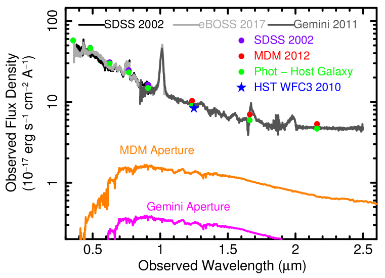
Figure 27: The inferred contribution of the host galaxy to the MDM photometry and the Gemini spectroscopy. The eBOSS spectrum was normalized to the SDSS spectrum, and then the Gemini spectrum was normalized to the result, taking advantage of the bright H$\alpha$ line which is present in both the eBOSS and Gemini spectra. The host galaxy is illustrated with a 5 Gyr-old template (Polletta et al., 2007), redshifted to the observed frame and reddened for Milky Way attenuation, and then scaled with the aperture fluxes listed in Table 3. We conclude that the host galaxy contributes negligibly to the continuum in Gemini spectrum in the region of the He I*$\lambda 10830$ absorption line.

B.3 How Does the Host Galaxy in SDSS J0850+4451 Compare with Other Quasar Host Galaxies?

As a final check of our analysis, we briefly compare the host galaxy properties with those from other low-redshift quasars. For a fair comparison, we recall the estimated black hole mass of $1.6\times 10^{9}\rm\,M_{\odot}$ from Paper I.

Bentz et al. (2009a, b) analyze HST images from reverberation-mapped AGN and quasars. All of these objects have smaller black hole masses than estimated for SDSS J0850+4451 ($\log M_{bh}=9.2$), but several objects are close, including PG 0804$+$761, PG 1226$+$023, PG 1426$+$015, and PG 1700$+$518, which have log black hole masses of 8.84, 8.95, 9.11, and 8.89, respectively. We compared the derived properties of SDSS J0850$+$4451 with those obtained for these four galaxies. The Sersic radial scale factor, between $\sim 4$ and $\sim 11\rm\,kpc$, is similar to the four comparison objects, which have scale factors between 3.3 to 12 kpc. The best fitting Sersic index is very low for SDSS J0850$+$4511, between 0.2 and 0.5 for the smaller component, and fixed to 1 for the larger component. This may not be physical, noting that the inner region is not well constrained due to the PSF. The indices for the comparison sample range from 1.0 to 5.6. Integrating over the template scaled to the total galaxy model flux and shifted into the rest frame yields a total log luminosity of $10.9\rm\,[L_{\odot}]$, which is again similar to the values of the comparison sample, which range from 10.6 to $11.2\rm\,[L_{\odot}]$ (Bentz et al., 2009b).

Landt et al. (2011, their Figure 1) present a graph showing the enclosed luminosity density at 5100Å rest frame from a sample of galaxies as a function of the extraction aperture. At the redshift of SDSS J0850+4451, the Gemini GNIRS aperture encloses $31.7\rm\,kpc^{2}$. The log luminosity density at 5100Å obtained from the scaled 5-Gyr-old elliptical template was $39.8\rm\,[erg\,s^{-1}$Å${}^{-1}]$. This lies approximately 0.35 dex lower than the regression line in Landt et al. (2011) Figure 1, corresponding to a factor of $\sim 2$, but within the scatter around the regression line.

We therefore conclude that the host galaxy in SDSS J0850$+$4511 is in no way anomalous but is instead typical of a galaxy in a low-redshift quasar, and that our conclusion that the host galaxy contribution to the continuum under the He I*$\lambda 10830$ line is negligible is robust.

References

- Arav et al. (2005) Arav, N., Kaastra, J., Kriss, G. A., et al. 2005, ApJ, 620, 665
- Arav et al. (2008) Arav, N., Moe, M., Costantini, E., et al. 2008, ApJ, 681, 954
- Bentz et al. (2009a) Bentz, M. C., Peterson, B. M., Netzer, H., Pogge, R. W., & Vestergaard, M. 2009a, ApJ, 697, 160
- Bentz et al. (2009b) Bentz, M. C., Peterson, B. M., Pogge, R. W., & Vestergaard, M. 2009b, ApJ, 694, L166
- Bentz et al. (2013) Bentz, M. C., Denney, K. D., Grier, C. J., et al. 2013, ApJ, 767, 149
- Borguet et al. (2013) Borguet, B. C. J., Arav, N., Edmonds, D., Chamberlain, C., & Benn, C. 2013, ApJ, 762, 49
- Borguet et al. (2012) Borguet, B. C. J., Edmonds, D., Arav, N., Benn, C., & Chamberlain, C. 2012, ApJ, 758, 69
- Boroson (2002) Boroson, T. A. 2002, ApJ, 565, 78
- Canalizo et al. (2007) Canalizo, G., Bennert, N., Jungwiert, B., et al. 2007, ApJ, 669, 801
- Capellupo et al. (2013) Capellupo, D. M., Hamann, F., Shields, J. C., Halpern, J. P., & Barlow, T. A. 2013, MNRAS, 429, 1872
- Capellupo et al. (2011) Capellupo, D. M., Hamann, F., Shields, J. C., Rodríguez Hidalgo, P., & Barlow, T. A. 2011, MNRAS, 413, 908
- Capellupo et al. (2012) —. 2012, MNRAS, 422, 3249
- Capellupo et al. (2017) Capellupo, D. M., Hamann, F., Herbst, H., et al. 2017, MNRAS, 469, 323
- Casebeer et al. (2006) Casebeer, D. A., Leighly, K. M., & Baron, E. 2006, ApJ, 637, 157
- Chamberlain et al. (2015) Chamberlain, C., Arav, N., & Benn, C. 2015, MNRAS, 450, 1085
- Clegg (1987) Clegg, R. E. S. 1987, MNRAS, 229, 31P
- Colless et al. (2001) Colless, M., Dalton, G., Maddox, S., et al. 2001, MNRAS, 328, 1039
- Collier et al. (1998) Collier, S. J., Horne, K., Kaspi, S., et al. 1998, ApJ, 500, 162
- Cushing et al. (2004) Cushing, M. C., Vacca, W. D., & Rayner, J. T. 2004, PASP, 116, 362
- de Kool et al. (2002) de Kool, M., Korista, K. T., & Arav, N. 2002, ApJ, 580, 54
- Depoy et al. (1993) Depoy, D. L., Atwood, B., Byard, P. L., Frogel, J., & O’Brien, T. P. 1993, in Proc. SPIE, Vol. 1946, Infrared Detectors and Instrumentation, ed. A. M. Fowler, 667–672
- DiPompeo et al. (2013) DiPompeo, M. A., Brotherton, M. S., & De Breuck, C. 2013, MNRAS, 428, 1565
- Done et al. (2012) Done, C., Davis, S. W., Jin, C., Blaes, O., & Ward, M. 2012, MNRAS, 420, 1848
- Dunn et al. (2010) Dunn, J. P., Bautista, M., Arav, N., et al. 2010, ApJ, 709, 611
- Ferland et al. (2013) Ferland, G. J., Porter, R. L., van Hoof, P. A. M., et al. 2013, Rev. Mexicana Astron. Astrofis., 49, 137
- Filiz Ak et al. (2013) Filiz Ak, N., Brandt, W. N., Hall, P. B., et al. 2013, ApJ, 777, 168
- Finn et al. (2014) Finn, C. W., Morris, S. L., Crighton, N. H. M., et al. 2014, MNRAS, 440, 3317
- Foreman-Mackey et al. (2013) Foreman-Mackey, D., Hogg, D. W., Lang, D., & Goodman, J. 2013, PASP, 125, 306
- Frank et al. (2002) Frank, J., King, A., & Raine, D. J. 2002, Accretion Power in Astrophysics: Third Edition
- Freeman et al. (2001) Freeman, P., Doe, S., & Siemiginowska, A. 2001, in Society of Photo-Optical Instrumentation Engineers (SPIE) Conference Series, Vol. 4477, Society of Photo-Optical Instrumentation Engineers (SPIE) Conference Series, ed. J.-L. Starck & F. D. Murtagh, 76–87
- Gabel et al. (2005) Gabel, J. R., Kraemer, S. B., Crenshaw, D. M., et al. 2005, ApJ, 631, 741
- Ganguly et al. (2013) Ganguly, R., Lynch, R. S., Charlton, J. C., et al. 2013, MNRAS, 435, 1233
- Gibson et al. (2009) Gibson, R. R., Jiang, L., Brandt, W. N., et al. 2009, ApJ, 692, 758
- Grevesse et al. (2007) Grevesse, N., Asplund, M., & Sauval, A. J. 2007, Space Sci. Rev., 130, 105
- Grupe et al. (2013) Grupe, D., Komossa, S., Scharwächter, J., et al. 2013, AJ, 146, 78
- Hall et al. (2003) Hall, P. B., Hutsemékers, D., Anderson, S. F., et al. 2003, ApJ, 593, 189
- Hamann (1998) Hamann, F. 1998, ApJ, 500, 798
- Hamann et al. (1997) Hamann, F., Barlow, T. A., Junkkarinen, V., & Burbidge, E. M. 1997, ApJ, 478, 80
- Hamann et al. (2011) Hamann, F., Kanekar, N., Prochaska, J. X., et al. 2011, MNRAS, 410, 1957
- Hamann et al. (2002) Hamann, F., Korista, K. T., Ferland, G. J., Warner, C., & Baldwin, J. 2002, ApJ, 564, 592
- Hamann et al. (2001) Hamann, F. W., Barlow, T. A., Chaffee, F. C., Foltz, C. B., & Weymann, R. J. 2001, ApJ, 550, 142
- Hao et al. (2011) Hao, H., Elvis, M., Civano, F., & Lawrence, A. 2011, ApJ, 733, 108
- Hao et al. (2010) Hao, H., Elvis, M., Civano, F., et al. 2010, ApJ, 724, L59
- Hopkins & Elvis (2010) Hopkins, P. F., & Elvis, M. 2010, MNRAS, 401, 7
- Jester et al. (2005) Jester, S., Schneider, D. P., Richards, G. T., et al. 2005, AJ, 130, 873
- Kalirai et al. (2009) Kalirai, J. S., MacKenty, J., Bohlin, R., et al. 2009, WFC3 SMOV Proposal 11451: The Photometric Performance and Calibration of WFC3/IR, Tech. rep.
- Kishimoto et al. (2007) Kishimoto, M., Hönig, S. F., Beckert, T., & Weigelt, G. 2007, A&A, 476, 713
- Korista et al. (1997) Korista, K., Baldwin, J., Ferland, G., & Verner, D. 1997, ApJS, 108, 401
- Krawczyk et al. (2015) Krawczyk, C. M., Richards, G. T., Gallagher, S. C., et al. 2015, AJ, 149, 203
- Landt et al. (2011) Landt, H., Elvis, M., Ward, M. J., et al. 2011, MNRAS, 414, 218
- Leighly et al. (2019) Leighly, K., Terndrup, D., Gallagher, S. C., & Richards, G. 2019, in American Astronomical Society Meeting Abstracts, Vol. 233, American Astronomical Society Meeting Abstracts #233, 242.39
- Leighly et al. (2015) Leighly, K. M., Cooper, E., Grupe, D., Terndrup, D. M., & Komossa, S. 2015, ApJ, 809, L13
- Leighly et al. (2011) Leighly, K. M., Dietrich, M., & Barber, S. 2011, ApJ, 728, 94
- Leighly et al. (2007) Leighly, K. M., Halpern, J. P., Jenkins, E. B., & Casebeer, D. 2007, ApJS, 173, 1
- Leighly et al. (2009) Leighly, K. M., Hamann, F., Casebeer, D. A., & Grupe, D. 2009, ApJ, 701, 176
- Leighly & Moore (2006) Leighly, K. M., & Moore, J. R. 2006, ApJ, 644, 748
- Leighly et al. (2018) Leighly, K. M., Terndrup, D. M., Gallagher, S. C., Richards, G. T., & Dietrich, M. 2018, ArXiv e-prints
- Lira et al. (2018) Lira, P., Kaspi, S., Netzer, H., et al. 2018, ArXiv e-prints
- Lucy et al. (2014) Lucy, A. B., Leighly, K. M., Terndrup, D. M., Dietrich, M., & Gallagher, S. C. 2014, ApJ, 783, 58
- Luo et al. (2013) Luo, B., Brandt, W. N., Alexander, D. M., et al. 2013, ApJ, 772, 153
- Lyu et al. (2017) Lyu, J., Rieke, G. H., & Shi, Y. 2017, ApJ, 835, 257
- Margala et al. (2016) Margala, D., Kirkby, D., Dawson, K., et al. 2016, ApJ, 831, 157
- Martini et al. (2014) Martini, P., Elias, J., Points, S., et al. 2014, in Proc. SPIE, Vol. 9147, Ground-based and Airborne Instrumentation for Astronomy V, 91470Z
- McGraw et al. (2015) McGraw, S. M., Shields, J. C., Hamann, F. W., et al. 2015, MNRAS, 453, 1379
- McGraw et al. (2018) McGraw, S. M., Shields, J. C., Hamann, F. W., Capellupo, D. M., & Herbst, H. 2018, MNRAS, 475, 585
- Misawa et al. (2007) Misawa, T., Charlton, J. C., Eracleous, M., et al. 2007, ApJS, 171, 1
- Moe et al. (2009) Moe, M., Arav, N., Bautista, M. A., & Korista, K. T. 2009, ApJ, 706, 525
- Moravec et al. (2017) Moravec, E. A., Hamann, F., Capellupo, D. M., et al. 2017, MNRAS, 468, 4539
- Ogle et al. (1999) Ogle, P. M., Cohen, M. H., Miller, J. S., et al. 1999, ApJS, 125, 1
- Onken & Peterson (2002) Onken, C. A., & Peterson, B. M. 2002, ApJ, 572, 746
- Peterson & Wandel (1999) Peterson, B. M., & Wandel, A. 1999, ApJ, 521, L95
- Polletta et al. (2007) Polletta, M., Tajer, M., Maraschi, L., et al. 2007, ApJ, 663, 81
- Richards et al. (2006) Richards, G. T., Lacy, M., Storrie-Lombardi, L. J., et al. 2006, ApJS, 166, 470
- Riess (2011) Riess, A. G. 2011, An Independent Determination of WFC3-IR Zeropoints and Count Rate Non-Linearity from 2MASS Asterisms, Tech. rep.
- Rodríguez Hidalgo et al. (2011) Rodríguez Hidalgo, P., Hamann, F., & Hall, P. 2011, MNRAS, 411, 247
- Sabra & Hamann (2001) Sabra, B. M., & Hamann, F. 2001, ApJ, 563, 555
- Sabra & Hamann (2005) —. 2005, ArXiv Astrophysics e-prints
- Savage & Sembach (1991) Savage, B. D., & Sembach, K. R. 1991, ApJ, 379, 245
- Schlafly & Finkbeiner (2011) Schlafly, E. F., & Finkbeiner, D. P. 2011, ApJ, 737, 103
- Vacca et al. (2003) Vacca, W. D., Cushing, M. C., & Rayner, J. T. 2003, PASP, 115, 389
- Vestergaard & Peterson (2006) Vestergaard, M., & Peterson, B. M. 2006, ApJ, 641, 689
- Vivek et al. (2014) Vivek, M., Srianand, R., Petitjean, P., et al. 2014, MNRAS, 440, 799
- Wanders et al. (1997) Wanders, I., Peterson, B. M., Alloin, D., et al. 1997, ApJS, 113, 69
- Weymann et al. (1991) Weymann, R. J., Morris, S. L., Foltz, C. B., & Hewett, P. C. 1991, ApJ, 373, 23