Dual Latent Variable Model for Low-Resource Natural Language Generation in Dialogue Systems

Abstract

Recent deep learning models have shown improving results to natural language generation (NLG) irrespective of providing sufficient annotated data. However, a modest training data may harm such models’ performance. Thus, how to build a generator that can utilize as much of knowledge from a low-resource setting data is a crucial issue in NLG. This paper presents a variational neural-based generation model to tackle the NLG problem of having limited labeled dataset, in which we integrate a variational inference into an encoder-decoder generator and introduce a novel auxiliary auto-encoding with an effective training procedure. Experiments showed that the proposed methods not only outperform the previous models when having sufficient training dataset but also show strong ability to work acceptably well when the training data is scarce.

1 Introduction

Natural language generation (NLG) plays an critical role in Spoken dialogue systems (SDSs) with the NLG task is mainly to convert a meaning representation produced by the dialogue manager, i.e., dialogue act (DA), into natural language responses. SDSs are typically developed for various specific domains, i.e., flight reservations Levin et al. (2000), buying a tv or a laptop Wen et al. (2015b), searching for a hotel or a restaurant Wen et al. (2015a), and so forth. Such systems often require well-defined ontology datasets that are extremely time-consuming and expensive to collect. There is, thus, a need to build NLG systems that can work acceptably well when the training data is in short supply.

There are two potential solutions for above-mentioned problems, which are domain adaptation training and model designing for low-resource training. First, domain adaptation training which aims at learning from sufficient source domain a model that can perform acceptably well on a different target domain with a limited labeled target data. Domain adaptation generally involves two different types of datasets, one from a source domain and the other from a target domain. Despite providing promising results for low-resource setting problems, the methods still need an adequate training data at the source domain site.

Second, model designing for low-resource setting has not been well studied in the NLG literature. The generation models have achieved very good performances irrespective of providing sufficient labeled datasets Wen et al. (2015b, a); Tran et al. (2017); Tran and Nguyen (2017). However, small training data easily result in worse generation models in the supervised learning methods. Thus, this paper presents an explicit way to construct an effective low-resource setting generator.

In summary, we make the following contributions, in which we: (i) propose a variational approach for an NLG problem which benefits the generator to not only outperform the previous methods when there is a sufficient training data but also perform acceptably well regarding low-resource data; (ii) present a variational generator that can also adapt faster to a new, unseen domain using a limited amount of in-domain data; (iii) investigate the effectiveness of the proposed method in different scenarios, including ablation studies, scratch, domain adaptation, and semi-supervised training with varied proportion of dataset.

2 Related Work

Recently, the RNN-based generators have shown improving results in tackling the NLG problems in task oriented-dialogue systems with varied proposed methods, such as HLSTM Wen et al. (2015a), SCLSTM Wen et al. (2015b), or especially RNN Encoder-Decoder models integrating with attention mechanism, such as Enc-Dec Wen et al. (2016b), and RALSTM Tran and Nguyen (2017). However, such models have proved to work well only when providing a sufficient in-domain data since a modest dataset may harm the models’ performance.

In this context, one can think of a potential solution where the domain adaptation learning is utilized. The source domain, in this scenario, typically contains a sufficient amount of annotated data such that a model can be efficiently built, while there is often little or no labeled data in the target domain. A phrase-based statistical generator Mairesse et al. (2010) using graphical models and active learning, and a multi-domain procedure Wen et al. (2016a) via data counterfeiting and discriminative training. However, a question still remains as how to build a generator that can directly work well on a scarce dataset.

Neural variational framework for generative models of text have been studied extensively. Chung et al. (2015) proposed a recurrent latent variable model for sequential data by integrating latent random variables into hidden state of an RNN. A hierarchical multi scale recurrent neural networks was proposed to learn both hierarchical and temporal representation Chung et al. (2016), while Bowman et al. (2015) presented a variational autoencoder for unsupervised generative language model. Sohn et al. (2015) proposed a deep conditional generative model for structured output prediction, whereas Zhang et al. (2016) introduced a variational neural machine translation that incorporated a continuous latent variable to model underlying semantics of sentence pairs. To solve the exposure-bias problem Bengio et al. (2015) Zhang et al. (2017); Shen et al. (2017) proposed a seq2seq purely convolutional and deconvolutional autoencoder, Yang et al. (2017) proposed to use a dilated CNN decoder in a latent-variable model, or Semeniuta et al. (2017) proposed a hybrid VAE architecture with convolutional and deconvolutional components.

3 Dual Latent Variable Model

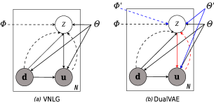
Figure 1: Illustration of proposed variational models as a directed graph. (a) VNLG: joint learning both variational parameters $\phi$ and generative model parameters $\theta$. (b) DualVAE: red and blue arrows form a standard VAE (parameterized by $\phi^{\prime}$ and $\theta^{\prime}$) as an auxiliary auto-encoding to the VNLG model denoted by red and black arrows.

3.1 Variational Natural Language Generator

We make an assumption about the existing of a continuous latent variable $z$ from a underlying semantic space of DA-Utterance pairs $(\textbf{d},\textbf{u})$, so that we explicitly model the space together with variable d to guide the generation process, i.e., $p(\textbf{u}|z,\textbf{d})$. The original conditional probability $p(\textbf{y}|\textbf{d})$ modeled by a vanilla encoder-decoder network is thus reformulated as follows:

$$p(\textbf{u}|\textbf{d})=\int_{z}p(\textbf{u},z|\textbf{d})\textbf{d}_{z}=\int_{z}p(\textbf{u}|z,\textbf{d})p(z|\textbf{d})\textbf{d}_{z}$$ (1)

This latent variable enables us to model the underlying semantic space as a global signal for generation. However, the incorporating of latent variable into the probabilistic model arises two difficulties in (i) modeling the intractable posterior inference $p(z|\textbf{d},\textbf{u})$ and (ii) whether or not the latent variables $z$ can be modeled effectively in case of low-resource setting data.

To address the difficulties, we propose an encoder-decoder based variational model to natural language generation (VNLG) by integrating a variational autoencoder Kingma and Welling (2013) into an encoder-decoder generator Tran and Nguyen (2017). Figure 1-(a) shows a graphical model of VNLG. We then employ deep neural networks to approximate the prior $p(z|\textbf{d})$, true posterior $p(z|\textbf{d},\textbf{u})$, and decoder $p(\textbf{u}|z,\textbf{d})$. To tackle the first issue, the intractable posterior is approximated from both the DA and utterance information $q_{\phi}(z|\textbf{d},\textbf{u})$ under the above assumption. In contrast, the prior is modeled to condition on the DA only $p_{\theta}(z|\textbf{d})$ due to the fact that the DA and utterance of a training pair usually share the same semantic information, i.e., a given DA inform(name=‘ABC’; area=‘XYZ’) contains key information of the corresponding utterance “The hotel ABC is in XYZ area”. The underlying semantic space with having more information encoded from both the prior and the posterior provides the generator a potential solution to tackle the second issue. Lastly, in generative process, given an observation DA d the output u is generated by the decoder network $p_{\theta}(\textbf{u}|z,\textbf{d})$ under the guidance of the global signal $z$ which is drawn from the prior distribution $p_{\theta}(z|\textbf{d})$. According to Sohn et al. (2015), the variational lower bound can be recomputed as:

$$\mathcal{L}(\theta, \phi,\textbf{d},\textbf{u})=-KL(q_{\phi}(z|\textbf{d},\textbf{u})||p_{\theta}(z|\textbf{d}))$$ (2)

$$+ \mathbb{E}_{q_{\phi}(z|\textbf{d},\textbf{u})}[\log p_{\theta}(\textbf{u}|z,\textbf{d})]\leq\log p(\textbf{u}|\textbf{d})$$

3.1.1 Variational Encoder Network

The encoder consists of two networks: (i) a Bidirectional LSTM (BiLSTM) which encodes the sequence of slot-value pairs $\{{\textbf{sv}}_{i}\}^{T_{DA}}_{i=1}$ by separate parameterization of slots and values Wen et al. (2016b); and (ii) a shared CNN/RNN Utterance Encoder which encodes the corresponding utterance. The encoder network, thus, produces both the DA representation $\textbf{h}_{\textbf{D}}$ and the utterance representation $\textbf{h}_{\textbf{U}}$ vectors which flow into the inference and decoder networks, and the posterior approximator, respectively (see Suppl. 1.1).

3.1.2 Variational Inference Network

This section models both the prior $p_{\theta}(z|\textbf{d})$ and the posterior $q_{\phi}(z|\textbf{d},\textbf{u})$ by utilizing neural networks.

Neural Posterior Approximator: We approximate the intractable posterior distribution of $z$ to simplify the posterior inference, in which we first projects both DA and utterance representations onto the latent space:

$$\textbf{h}^{\prime}_{z}=g(\textbf{W}_{z}[\textbf{h}_{\textbf{D}};\textbf{h}_{\textbf{U}}]+b_{z})\vspace{-5pt}$$ (3)

where $\textbf{W}_{z}\in\mathbb{R}^{d_{z}\times(d_{\textbf{h}_{\textbf{D}}}+d_{\textbf{h}_{\textbf{U}}})}$, $b_{z}\in\mathbb{R}^{d_{z}}$ are matrix and bias parameters respectively, $d_{z}$ is the dimensionality of the latent space, and we set $g(.)$ to be ReLU in our experiments. We then approximate the posterior as:

$$q_{\phi}(z|\textbf{d},\textbf{u})=\mathcal{N}(z;\mu_{1}(\textbf{h}^{\prime}_{z}),\sigma_{1}^{2}(\textbf{h}^{\prime}_{z})\textbf{{I}})$$ (4)

with mean $\mu_{1}$ and standard variance $\sigma_{1}$ are the outputs of the neural network as follows:

$$\mu_{1}=\textbf{W}_{\mu_{1}}\textbf{h}^{\prime}_{z}+b_{\mu_{1}},\log\sigma_{1}^{2}=\textbf{W}_{\sigma_{1}}\textbf{h}^{\prime}_{z}+b_{\sigma_{1}}$$ (5)

where $\mu_{1}$, $\log\sigma_{1}^{2}$ are both $d_{z}$ dimension vectors.

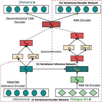
Figure 2: The Dual latent variable model consists of two VAE models: (i) a VNLG (red-dashed box) is to generate utterances and (ii) a Variational CNN-DCNN is an auxiliary auto-encoding model (left side). The RNN/CNN Utterance Encoder is shared between the two VAEs.

Neural Prior: We model the prior as follows:

$$p_{\theta}(z|\textbf{d})=\mathcal{N}(z;\mu^{\prime}_{1}(\textbf{d}),{\sigma^{\prime}}^{2}_{1}(\textbf{d})\textbf{{I}})$$ (6)

where $\mu_{1}^{\prime}$ and $\sigma_{1}^{\prime}$ of the prior are neural models only based on the Dialogue Act representation, which are the same as those of the posterior $q_{\phi}(z|\textbf{d},\textbf{u})$ in Eq. 3 and 5, except for the absence of $\textbf{h}_{\textbf{U}}$. To obtain a representation of the latent variable $z$, we re-parameterize it as follows: $\textbf{h}_{z}=\mu_{1}+\sigma_{1}\odot\epsilon$ where $\epsilon\sim\mathcal{N}(0,\textbf{{I}}).$

Note here that the parameters for the prior and the posterior are independent of each other. Moreover, during decoding we set $\textbf{h}_{z}$ to be the mean of the prior $p_{\theta}(z|\textbf{d})$, i.e., $\mu_{1}^{\prime}$ due to the absence of the utterance u. In order to integrate the latent variable $\textbf{h}_{z}$ into the decoder, we use a non-linear transformation to project it onto the output space for generation: $\textbf{h}_{e}=g(\textbf{W}_{e}\textbf{h}_{z}+b_{e})(7)$, where $\textbf{h}_{e}\in\mathbb{R}^{d_{e}}$.

3.1.3 Variational Decoder Network

Given a DA d and the latent variable $z$, the decoder calculates the probability over the generation u as a joint probability of ordered conditionals:

$$p(\textbf{u}|z,\textbf{d})=\prod_{t=1}^{T_{\textbf{U}}}p(\textbf{u}_{t}|\textbf{u}_{<t},z,\textbf{d})$$ (8)

where $p(\textbf{u}_{t}|\textbf{u}_{<t},z,\textbf{d})$=$g^{\prime}(\textnormal{RALSTM}(\textbf{u}_{t},\textbf{h}_{t-1},\textbf{d}_{t})$. The RALSTM cell Tran and Nguyen (2017) is slightly modified in order to integrate the representation of latent variable, i.e., $\textbf{h}_{e}$, into the computational cell (see Suppl. 1.3), in which the latent variable can affect the hidden representation through the gates. This allows the model can indirectly take advantage of the underlying semantic information from the latent variable $z$. In addition, when the model learns unseen dialogue acts, the semantic representation $\textbf{h}_{e}$ can benefit the generation process (see Table 1).

We finally obtain the VNLG model with RNN Utterance Encoder (R-VNLG) or with CNN Utterance Encoder (C-VNLG).

3.2 Variational CNN-DCNN Model

This standard VAE model (left side in Figure 2) acts as an auxiliary auto-encoding for utterance (used at training time) to the VNLG generator. The model consists of two components. While the shared CNN Utterance Encoder with the VNLG model is to compute the latent representation vector $\textbf{h}_{\textbf{U}}$ (see Suppl. 1.1.3), a Deconvolutional CNN Decoder to decode the latent representation $\textbf{h}_{e}$ back to the source text (see Suppl. 2.1). Specifically, after having the vector representation $\textbf{h}_{\textbf{U}}$, we apply another linear regression to obtain the distribution parameter $\mu_{2}=\textbf{W}_{\mu_{2}}\textbf{h}_{\textbf{U}}+b_{\mu_{2}}$ and $\log\sigma_{2}^{2}=\textbf{W}_{\sigma_{2}}\textbf{h}_{\textbf{U}}+b_{\sigma_{2}}$. We then re-parameterize them to obtain a latent representation $\textbf{h}_{zu}=\mu_{2}+\sigma_{2}\odot\epsilon$, where $\epsilon\sim\mathcal{N}(0,\textbf{{I}})$. In order to integrate the latent variable $\textbf{h}_{zu}$ into the DCNN Decoder, we use the shared non-linear transformation as in Eq. 3.1.2 (denoted by the black-dashed line in Figure 2) as: $\textbf{h}_{e}=g(\textbf{W}_{e}\textbf{h}_{zu}+b_{e})$.

The entire resulting model, named DualVAE, by incorporating the VNLG with the Variational CNN-DCNN model, is depicted in Figure 2.

4 Training Dual Latent Variable Model

4.1 Training VNLG Model

Inspired by work of Zhang et al. (2016), we also employ the Monte-Carlo method to approximate the expectation of the posterior in Eq. 2, i.e. $\mathbb{E}_{q_{\phi}(z|\textbf{d},\textbf{u})}[.]\simeq\frac{1}{M}\sum_{m=1}^{M}\log p_{\theta}(\textbf{u}|\textbf{d},\textbf{h}_{z}^{(m)})$ where $M$ is the number of samples. In this work, the joint training objective $\mathcal{L}_{\textnormal{VNLG}}$ for a training instance pair $(\textbf{d},\textbf{u})$ is formulated as:

$$\mathcal{L}(\theta,\phi,\textbf{d},\textbf{u})\simeq-KL(q_{\phi}(z|\textbf{d},\textbf{u})||p_{\theta}(z|\textbf{d}))$$ (9)

$$+\frac{1}{M}\sum_{m=1}^{M}\sum_{t=1}^{T_{U}}\log p_{\theta}(\textbf{u}_{t}|\textbf{u}_{<t},\textbf{d},\textbf{h}_{z}^{(m)})$$

where $\textbf{h}_{z}^{(m)}=\mu+\sigma\odot\epsilon^{(m)}$, and $\epsilon^{(m)}\sim\mathcal{N}(0,\textbf{I})$, and $\theta$ and $\phi$ denote decoder and encoder parameters, respectively. The first term is the KL divergence between two Gaussian distribution, and the second term is the approximation expectation. We simply set $M=1$ which degenerates the second term to the objective of conventional generator. Since the objective function in Eq. 9 is differentiable, we can jointly optimize the parameter $\theta$ and variational parameter $\phi$ using standard gradient ascent techniques. However, the KL divergence loss tends to be significantly small during training Bowman et al. (2015). As a results, the decoder does not take advantage of information from the latent variable $z$. Thus, we apply the KL cost annealing strategy that encourages the model to encode meaningful representations into the latent vector $z$, in which we gradually anneal the KL term from $0$ to $1$. This helps our model to achieve solutions with non-zero KL term.

4.2 Training Variational CNN-DCNN Model

The objective function $\mathcal{L}_{\textnormal{CNN-DCNN}}$ of the Variational CNN-DCNN model is the standard VAE lower bound and maximized as follows:

$$\mathcal{L}(\theta^{\prime} ,\phi^{\prime},\textbf{u})=-KL(q_{\phi^{\prime}}(z|\textbf{u})||p_{\theta^{\prime}}(z))$$ (10)

$$+\mathbb{E}_{q_{\phi^{\prime}}(z|\textbf{u})}[\log p_{\theta^{\prime}}(\textbf{u}|z)]\leq\log p(\textbf{u})$$

where $\theta^{\prime}$ and $\phi^{\prime}$ denote decoder and encoder parameters, respectively. During training, we also consider a denoising autoencoder where we slightly modify the input by swapping some arbitrary word pairs.

4.3 Joint Training Dual VAE Model

To allow the model explore and balance maximizing the variational lower bound between the Variational CNN-DCNN model and VNLG model, an objective is joint training as follows:

$$\mathcal{L}_{\textnormal{{DualVAE}}}=\mathcal{L}_{\textnormal{VNLG}}+\alpha\mathcal{L}_{\textnormal{CNN-DCNN}}$$ (11)

where $\alpha$ controls the relative weight between two variational losses. During training, we anneal the value of $\alpha$ from $1$ to $0$, so that the dual latent variable learned can gradually focus less on reconstruction objective of the CNN-DCNN model, only retain those features that are useful for the generation objective.

4.4 Joint Cross Training Dual VAE Model

To allow the dual VAE model explore and encode useful information of the Dialogue Act into the latent variable, we further take a cross training between two VAEs by simply replacing the RALSTM Decoder of the VNLG model with the DCNN Utterance Decoder and its objective training $\mathcal{L}_{\textnormal{DA-DCNN}}$ as:

$$\mathcal{L}(\theta^{\prime},\phi,\textbf{d},\textbf{u}) \simeq-KL(q_{\phi}(z|\textbf{d},\textbf{u})||p_{\theta^{\prime}}(z|\textbf{d}))$$ (12)

$$+\mathbb{E}_{q_{\phi}(z|\textbf{d},\textbf{u})}[\log p_{\theta^{\prime}}(\textbf{u}|z,\textbf{d})],$$

and a joint cross training objective is employed:

$$\mathcal{L}_{\textnormal{{CrossVAE}}} =\mathcal{L}_{\textnormal{VNLG}}$$ (13)

$$+\alpha(\mathcal{L}_{\textnormal{CNN-DCNN}}+\mathcal{L}_{\textnormal{DA-DCNN}})$$

5 Experiments

We assessed the proposed models on four different original NLG domains: finding a restaurant and hotel Wen et al. (2015a), or buying a laptop and television Wen et al. (2016b).

5.1 Evaluation Metrics and Baselines

The generator performances were evaluated using the two metrics: the BLEU and the slot error rate ERR by adopting code from an NLG toolkit. We compared the proposed models against strong baselines which have been recently published as NLG benchmarks of those datasets, including (i) gating models such as HLSTM Wen et al. (2015a), and SCLSTM Wen et al. (2015b); and (ii) attention models such as Enc-Dec Wen et al. (2016b), RALSTM Tran and Nguyen (2017).

5.2 Experimental Setups

In this work, the CNN Utterance Encoder consists of $L=3$ layers, which for a sentence of length $T=73$, embedding size $d=100$, stride length $s=\{2,2,2\}$, number of filters $k=\{300,600,100\}$ with filter sizes $h=\{5,5,16\}$, results in feature maps V of sizes $\{35\times 300,16\times 600,1\times 100\}$, in which the last feature map corresponds to latent representation vector $\textbf{h}_{\textbf{U}}$.

The hidden layer size and beam width were set to be $100$ and $10$, respectively, and the models were trained with a $70\%$ of keep dropout rate. We performed $5$ runs with different random initialization of the network, and the training process is terminated by using early stopping. For the variational inference, we set the latent variable size to be $300$. We used Adam optimizer with the learning rate is initially set to be $0.001$, and after $5$ epochs the learning rate is decayed every epoch using an exponential rate of $0.95$.

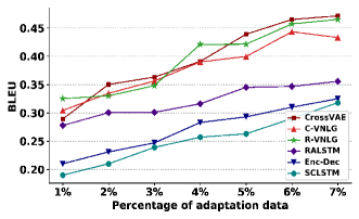
Figure 3: Performance on Laptop domain with varied limited amount, from 1% to 7%, of the adaptation training data when adapting models pre-trained on [Restaurant+Hotel] union dataset.

6 Results and Analysis

We performed the models in different scenarios as follows: (i) scratch training where models trained from scratch using $10$% (scr10), $30$% (scr30), and $100$% (scr100) amount of in-domain data; and (ii) domain adaptation training where models pre-trained from scratch using all source domain data, then fine-tuned on the target domain using only $10\%$ amount of the target data. Overall, the proposed models can work well in scenarios of low-resource setting data. The proposed models obtained state-of-the-art performances regarding both the evaluation metrics across all domains in all training scenarios.

	Model	Hotel		Restaurant		Tv		Laptop
		BLEU	ERR	BLEU	ERR	BLEU	ERR	BLEU	ERR
scr100	HLSTM	0.8488	2.79%	0.7436	0.85%	0.5240	2.65%	0.5130	1.15%
	SCLSTM	0.8469	3.12%	0.7543	0.57%	0.5235	2.41%	0.5109	0.89%
	ENCDEC	0.8537	4.78%	0.7358	2.98%	0.5142	3.38%	0.5101	4.24%
	RALSTM	0.8965	0.58%	0.7779	0.20%	0.5373	0.49%	0.5231	0.50%
	R-VNLG (Ours)	0.8851	0.57%	0.7709	0.36%	0.5356	0.73%	0.5210	0.59%
	C-VNLG (Ours)	0.8811	0.49%	0.7651	0.06%	0.5350	0.88%	0.5192	0.56%
	DualVAE (Ours)	0.8813	0.33%	0.7695	0.29%	0.5359	0.81%	0.5211	0.91%
	CrossVAE (Ours)	0.8926	0.72%	0.7786	0.54%	0.5383	0.48%	0.5240	0.50%
scr10	HLSTM	0.7483	8.69%	0.6586	6.93%	0.4819	9.39%	0.4813	7.37%
	SCLSTM	0.7626	17.42%	0.6446	16.93%	0.4290	31.87%	0.4729	15.89%
	ENCDEC	0.7370	23.19%	0.6174	23.63%	0.4570	21.28%	0.4604	29.86%
	RALSTM	0.6855	22.53%	0.6003	17.65%	0.4009	22.37%	0.4475	24.47%
	R-VNLG (Ours)	0.7378	15.43%	0.6417	15.69%	0.4392	17.45%	0.4851	10.06%
	C-VNLG (Ours)	0.7998	8.67%	0.6838	6.86%	0.5040	5.31%	0.4932	3.56%
	DualVAE (Ours)	0.8022	6.61%	0.6926	7.69%	0.5110	3.90%	0.5016	2.44%
	CrossVAE (Ours)	0.8103	6.20%	0.6969	4.06%	0.5152	2.86%	0.5085	2.39%
scr30	HLSTM	0.8104	6.39%	0.7044	2.13%	0.5024	5.82%	0.4859	6.70%
	SCLSTM	0.8271	6.23%	0.6825	4.80%	0.4934	7.97%	0.5001	3.52%
	ENCDEC	0.7865	9.38%	0.7102	13.47%	0.5014	9.19%	0.4907	10.72%
	RALSTM	0.8334	4.23%	0.7145	2.67%	0.5124	3.53%	0.5106	2.22%
	C-VNLG (Ours)	0.8553	2.64%	0.7256	0.96%	0.5265	0.66%	0.5117	2.15%
	DualVAE (Ours)	0.8534	1.54%	0.7301	2.32%	0.5288	1.05%	0.5107	0.93%
	CrossVAE (Ours)	0.8585	1.37%	0.7479	0.49%	0.5307	0.82%	0.5154	0.81%

Table 1: Results evaluated on four domains by training models from scratch with 10%, 30%, and 100% in-domain data, respectively. The results were averaged over 5 randomly initialized networks. The bold and italic faces denote the best and second best models in each training scenario, respectively.

6.1 Integrating Variational Inference

We compare the encoder-decoder RALSTM model to its modification by integrating with variational inference (R-VNLG and C-VNLG) as demonstrated in Figure 3 and Table 1.

It clearly shows that the variational generators not only provide a compelling evidence on adapting to a new, unseen domain when the target domain data is scarce, i.e., from $1$% to $7$% (Figure 3) but also preserve the power of the original RALSTM on generation task since their performances are very competitive to those of RALSTM (Table 1, scr100). Table 1, scr10 further shows the necessity of the integrating in which the VNLGs achieved a significant improvement over the RALSTM in scr10 scenario where the models trained from scratch with only a limited amount of training data ($10$%). These indicate that the proposed variational method can learn the underlying semantic of the existing DA-utterance pairs, which are especially useful information for low-resource setting.

Furthermore, the R-VNLG model has slightly better results than the C-VNLG when providing sufficient training data in scr100. In contrast, with a modest training data, in scr10, the latter model demonstrates a significant improvement compared to the former in terms of both the BLEU and ERR scores by a large margin across all four dataset. Take Hotel domain, for example, the C-VNLG model ($79.98$ BLEU, $8.67\%$ ERR) has better results in comparison to the R-VNLG ($73.78$ BLEU, $15.43\%$ ERR) and RALSTM ($68.55$ BLEU, $22.53\%$ ERR). Thus, the rest experiments focus on the C-VNLG since it shows obvious sign for constructing a dual latent variable models dealing with low-resource in-domain data. We leave the R-VNLG for future investigation.

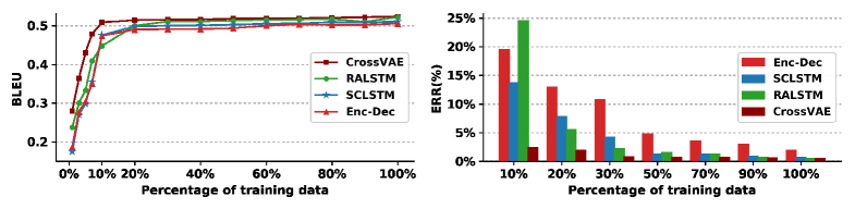
Figure 4: Performance comparison of the models trained on Laptop domain.

6.2 Ablation Studies

The ablation studies (Table 1) demonstrate the contribution of each model components, in which we incrementally train the baseline RALSTM, the C-VNLG (= RALSTM + Variational inference), the DualVAE (= C-VNLG + Variational CNN-DCNN), and the CrossVAE (= DualVAE + Cross training) models. Generally, while all models can work well when there are sufficient training datasets, the performances of the proposed models also increase as increasing the model components. The trend is consistent across all training cases no matter how much the training data was provided. Take, for example, the scr100 scenario in which the CrossVAE model mostly outperformed all the previous strong baselines with regard to the BLEU and the slot error rate ERR scores.

On the other hand, the previous methods showed extremely impaired performances regarding low BLEU score and high slot error rate ERR when training the models from scratch with only $10\%$ of in-domain data (scr10). In contrast, by integrating the variational inference, the C-VNLG model, for example in Hotel domain, can significantly improve the BLEU score from $68.55$ to $79.98$, and also reduce the slot error rate ERR by a large margin, from $22.53$ to $8.67$, compared to the RALSTM baseline. Moreover, the proposed models have much better performance over the previous ones in the scr10 scenario since the CrossVAE, and the DualVAE models mostly obtained the best and second best results, respectively. The CrossVAE model trained on scr10 scenario, in some cases, achieved results which close to those of the HLSTM, SCLSTM, and ENCDEC models trained on all training data (scr100) scenario. Take, for example, the most challenge dataset Laptop, in which the DualVAE and CrossVAE obtained competitive results regarding the BLEU score, at $50.16$ and $50.85$ respectively, which close to those of the HLSTM ($51.30$ BLEU), SCLSTM ($51.09$ BLEU), and ENCDEC ($51.01$ BLEU), while the results regardless the slot error rate ERR scores are also close to those of the previous or even better in some cases, for example DualVAE ($2.44$ ERR), CrossVAE ($2.39$ ERR), and ENCDEC ($4.24$ ERR). There are also some cases in TV domain where the proposed models (in scr10) have results close to or better over the previous ones (trained on scr100). These indicate that the proposed models can encode useful information into the latent variable efficiently to better generalize to the unseen dialogue acts, addressing the second difficulty with low-resource data.

The scr30 section further confirms the effectiveness of the proposed methods, in which the CrossVAE and DualVAE still mostly rank the best and second-best models compared with the baselines. The proposed models also show superior ability in leveraging the existing small training data to obtain very good performances, which are in many cases even better than those of the previous methods trained on $100$% of in-domain data. Take Tv domain, for example, in which the CrossVAE in scr30 achieves a good result regarding BLEU and slot error rate ERR score, at $53.07$ BLEU and $0.82$ ERR, that are not only competitive to the RALSTM ($53.73$ BLEU, $0.49$ ERR), but also outperform the previous models in scr100 training scenario, such as HLSTM ($52.40$ BLEU, $2.65$ ERR), SCLSTM ($52.35$ BLEU, $2.41$ ERR), and ENCDEC ($51.42$ BLEU, $3.38$ ERR). This further indicates the need of the integrating with variational inference, the additional auxiliary auto-encoding, as well as the joint and cross training.

6.3 Model comparison on unseen domain

In this experiment, we trained four models (ENCDEC, SCLSTM, RALSTM, and CrossVAE) from scratch in the most difficult unseen Laptop domain with an increasingly varied proportion of training data, start from $1$% to $100$%. The results are shown in Figure 4. It clearly sees that the BLEU score increases and the slot error ERR decreases as the models are trained on more data. The CrossVAE model is clearly better than the previous models (ENCDEC, SCLSTM, RALSTM) in all cases. While the performance of the CrossVAE, RALSTM model starts to saturate around $30$% and $50$%, respectively, the ENCDEC model seems to continue getting better as providing more training data. The figure also confirms that the CrossVAE trained on $30$% of data can achieve a better performance compared to those of the previous models trained on $100$% of in-domain data.

	Hotel		Restaurant		Tv		Laptop
	BLEU	ERR	BLEU	ERR	BLEU	ERR	BLEU	ERR
Hotel♭	-	-	0.6243	11.20%	0.4325	29.12%	0.4603	22.52%
Restaurant♭	0.7329	29.97%	-	-	0.4520	24.34%	0.4619	21.40%
Tv♭	0.7030	25.63%	0.6117	12.78%	-	-	0.4794	11.80%
Laptop♭	0.6764	39.21%	0.5940	28.93%	0.4750	14.17%	-	-
Hotel♯	-	-	0.7138	2.91%	0.5012	5.83%	0.4949	1.97%
Restaurant♯	0.7984	4.04%	-	-	0.5120	3.26%	0.4947	1.87%
Tv♯	0.7614	5.82%	0.6900	5.93%	-	-	0.4937	1.91%
Laptop♯	0.7804	5.87%	0.6565	6.97%	0.5037	3.66%	-	-
Hotelξ	-	-	0.6926	3.56%	0.4866	11.99%	0.5017	3.56%
Restaurantξ	0.7802	3.20%	-	-	0.4953	3.10%	0.4902	4.05%
Tvξ	0.7603	8.69%	0.6830	5.73%	-	-	0.5055	2.86%
Laptopξ	0.7807	8.20%	0.6749	5.84%	0.4988	5.53%	-	-
CrossVAE (scr10)	0.8103	6.20%	0.6969	4.06%	0.5152	2.86%	0.5085	2.39%
CrossVAE (semi-U50-L10)	0.8144	6.12%	0.6946	3.94%	0.5158	2.95%	0.5086	1.31%

Table 2: Results evaluated on Target domains by adaptation training SCLSTM model from $100$% (denoted as $\flat$) of Source data, and the CrossVAE model from 30% (denoted as $\sharp$), 100% (denoted as $\xi$) of Source data. The scenario used only 10% amount of the Target domain data. The last two rows show results by training the CrossVAE model on the scr10 and semi-supervised learning, respectively.

6.4 Domain Adaptation

We further examine the domain scalability of the proposed methods by training the CrossVAE and SCLSTM models on adaptation scenarios, in which we first trained the models on out-of-domain data, and then fine-tuned the model parameters by using a small amount ($10$%) of in-domain data. The results are shown in Table 2.

Both SCLSTM and CrossVAE models can take advantage of “close” dataset pairs, i.e., Restaurant $\leftrightarrow$ Hotel, and Tv $\leftrightarrow$ Laptop, to achieve better performances compared to those of the “different” dataset pairs, i.e. Latop $\leftrightarrow$ Restaurant. Moreover, Table 2 clearly shows that the SCLSTM (denoted by $\flat$) is limited to scale to another domain in terms of having very low BLEU and high ERR scores. This adaptation scenario along with the scr10 and scr30 in Table 1 demonstrate that the SCLSTM can not work when having a low-resource setting of in-domain training data.

On the other hand, the CrossVAE model again show ability in leveraging the out-of-domain data to better adapt to a new domain. Especially in the case where Laptop, which is a most difficult unseen domain, is the target domain the CrossVAE model can obtain good results irrespective of low slot error rate ERR, around $1.90$%, and high BLEU score, around $50.00$ points. Surprisingly, the CrossVAE model trained on scr10 scenario in some cases achieves better performance compared to those in adaptation scenario first trained with $30$% out-of-domain data (denoted by $\sharp$) which is also better than the adaptation model trained on $100$% out-of-domain data (denoted by $\xi$).

Preliminary experiments on semi-supervised training were also conducted, in which we trained the CrossVAE model with the same $10$% in-domain labeled data as in the other scenarios and $50$% in-domain unlabeled data by keeping only the utterances u in a given input pair of dialogue act-utterance (d, u), denoted by semi-U50-L10. The results showed CrossVAE’s ability in leveraging the unlabeled data to achieve slightly better results compared to those in scratch scenario. All these stipulate that the proposed models can perform acceptably well in training cases of scratch, domain adaptation, and semi-supervised where the in-domain training data is in short supply.

Model	Generated Responses from TV Domain
DA 1	compare(name=‘typhon 45’; hdmiport=‘2’; family=‘l2’; name=‘hades 48’; hdmiport=‘4’; family=‘l7’)
Reference 1	Compared to typhon 45 which has 2 hdmi port -s and is in the L2 product family, hades 48 has 4 hdmi port -s and is in the L7 product family. Which one do you prefer ?
ENCDEC-10	the typhon 45 is in the l2 product family and has 2 hdmi port -s and is in the l7 product family with 4 hdmi port -s, the hades 48 is in the SLOT_FAMILY product family with a SLOT_AUDIO.
HLSTM-10	the typhon 45 is a great eco rating, the hades 48 is in the l2 family with 2 hdmi port -s. [l7 family] [4 hdmi port -s]
SCLSTM-10	the typhon 45 is the hades 48 with 2 hdmi port in the l2 family, the SLOT_NAME has 4 hdmi port -s and SLOT_HDMIPORT hdmi port. [l7 family]
C-VNLG-10	the typhon 45 has 2 hdmi port -s and the hades 48 is in the l2 family and has 4 hdmi port -s. [l7 family]
DualVAE-10	the typhon 45 has 2 hdmi port -s and is in the l2 family while the hades 48 has 4 hdmi port -s and is in the l7 family. [OK]
CrossVAE-10	the typhon 45 is in the l2 family with 2 hdmi port -s while the hades 48 has 4 hdmi port -s and is in the l7 family. [OK]
ENCDEC-30	the typhon 45 has 2 hdmi port -s, the hades 48 has 4 hdmi port -s, the SLOT_NAME has SLOT_HDMIPORT hdmi port. [l2 family] [l7 family]
HLSTM-30	the typhon 45 is in the l2 product family with 2 hdmi port -s, whereas the hades 48 has 4 hdmi port. [l7 family]
SCLSTM-30	the typhon 45 has 2 hdmi port -s, the hades 48 is in the l2 product family. [l7 family] [4 hdmi port -s]
C-VNLG-30	the typhon 45 has 2 hdmi port -s, the hades 48 is in the l2 product family and has 4 hdmi port -s in l7 family.
DualVAE-30	which do you prefer, the typhon 45 in the l2 product family with 2 hdmi port -s . the hades 48 is in the l7 family with 4 hdmi port -s. [OK]
CrossVAE-30	the typhon 45 has 2 hdmi port -s and in the l2 family while the hades 48 has 4 hdmi port -s and is in the l7 family. which item do you prefer. [OK]
DA 2	recommend(name=‘proteus 73’; type=‘television’; price=‘1500 dollars’; audio=‘nicam stereo’; hdmiport=‘2’)
Reference 2	proteus 73 is a nice television. its price is 1500 dollars, its audio is nicam stereo, and it has 2 hdmi port -s.
ENCDEC-10	the proteus 73 is a great television with a nicam stereo and 2 hdmi port -s [1500 dollars]
HLSTM-10	the proteus 73 is a television with 2 hdmi port -s and comes with a nicam stereo and costs 1500 dollars [OK]
SCLSTM-10	the proteus 73 is a nice television with nicam stereo and 2 hdmi port -s [1500 dollars]
C-VNLG-10	the proteus 73 television has a nicam stereo and 2 hdmi port -s and costs 1500 dollars [OK]
DualVAE-10	the proteus 73 television has a nicam stereo and 2 hdmi port -s and costs 1500 dollars [OK]
CrossVAE-10	the proteus 73 television has 2 hdmi port -s and a nicam stereo and costs 1500 dollars [OK]
ENCDEC-30	the proteus 73 television has 2 hdmi port -s and nicam stereo audio for 1500 dollars [OK]
HLSTM-30	the proteus 73 television has a nicam stereo and 2 hdmi port -s and is priced at 1500 dollars [OK]
SCLSTM-30	the proteus 73 is a nice television with nicam stereo and 2 hdmi port -s . it is priced at 1500 dollars [OK]
C-VNLG-30	the proteus 73 television has 2 hdmi port -s , nicam stereo audio , and costs 1500 dollars [OK]
DualVAE-30	the proteus 73 television has 2 hdmi port -s and nicam stereo audio and costs 1500 dollars [OK]
CrossVAE-30	the proteus 73 television has 2 hdmi port -s and nicam stereo audio and costs 1500 dollars [OK]

Table 3: Comparison of top Tv responses generated for different models in different scenarios. Errors are marked in colors ([missing], misplaced, redundant, wrong, spelling mistake information). [OK] denotes successful generation. Model-X where X is amount of training data, i.e. 10%, 30%, or 100%.

Model	Generated Responses from Laptop Domain
DA	compare(name=‘satellite pallas 21’; battery=‘4 hour’; drive=‘500 gb’; name=‘satellite dinlas 18’; battery=‘3.5 hour’; drive=‘1 tb’)
Reference	compared to satellite pallas 21 which can last 4 hour and has a 500 gb drive , satellite dinlas 18 can last 3.5 hour and has a 1 tb drive . which one do you prefer
Enc-Dec-10	the satellite pallas 21 has a 500 gb drive , the satellite dinlas 18 has a 4 hour battery life and a 3.5 hour battery life and a SLOT_BATTERY battery life and a 1 tb drive
HLSTM-10	the satellite pallas 21 has a 4 hour battery life and a 500 gb drive . which one do you prefer [satellite pallas 18] [3.5 hour battery] [1 tb drive]
SCLSTM-10	the satellite pallas 21 has a 4 hour battery , and has a 3.5 hour battery life and a 500 gb drive and a 1 tb drive [satellite dinlas 18]
C-VNLG-10	the satellite pallas 21 has a 500 gb drive and a 4 hour battery life . the satellite dinlas 18 has a 3.5 hour battery life and a SLOT_BATTERY battery life [1 tb drive]
DualVAE-10	the satellite pallas 21 has a 4 hour battery life and a 500 gb drive and the satellite dinlas 18 with a 3.5 hour battery life and is good for business computing . which one do you prefer [1 tb drive]
CrossVAE-10	the satellite pallas 21 with 500 gb and a 1 tb drive . the satellite dinlas 18 with a 4 hour battery and a SLOT_DRIVE drive . which one do you prefer [3.5 hour battery]
Enc-Dec-30	the satellite pallas 21 has a 500 gb drive with a 1 tb drive and is the satellite dinlas 18 with a SLOT_DRIVE drive for 4 hour -s . which one do you prefer [3.5 hour battery]
HLSTM-30	the satellite pallas 21 is a 500 gb drive with a 4 hour battery life . the satellite dinlas 18 has a 3.5 hour battery life . which one do you prefer [1 tb drive]
SCLSTM-30	the satellite pallas 21 has a 500 gb drive . the satellite dinlas 18 has a 4 hour battery life . the SLOT_NAME has a 3.5 hour battery life . which one do you prefer [1 tb drive]
C-VNLG-30	which one do you prefer the satellite pallas 21 with a 4 hour battery life , the satellite dinlas 18 has a 500 gb drive and a 3.5 hour battery life and a 1 tb drive . which one do you prefer
DualVAE-30	satellite pallas 21 has a 500 gb drive and a 4 hour battery life while the satellite dinlas 18 with a 3.5 hour battery life and a 1 tb drive . [OK]
CrossVAE-30	the satellite pallas 21 has a 500 gb drive with a 4 hour battery life . the satellite dinlas 18 has a 1 tb drive and a 3.5 hour battery life . which one do you prefer [OK]

Table 4: Comparison of top Laptop responses generated for different models in different scenarios. Errors are marked in colors ([missing], misplaced, redundant, wrong, spelling information). [OK] denotes successful generation. Model-X where X is amount of training data, i.e. 10%, 30%, or 100%.

6.5 Comparison on Generated Outputs

We present top responses generated for different scenarios from TV (Table 3) and Laptop (Table 4), which further show the effectiveness of the proposed methods.

On the one hand, previous models trained on scr10, scr30 scenarios produce a diverse range of the outputs’ error types, including missing, misplaced, redundant, wrong slots, or spelling mistake information, resulting in a very high score of the slot error rate ERR. The ENCDEC, HLSTM and SCLSTM models in Table 3-DA 1, for example, tend to generate outputs with redundant slots (i.e., SLOT_HDMIPORT, SLOT_NAME, SLOT_FAMILY), missing slots (i.e., [l7 family], [4 hdmi port -s]), or even in some cases produce irrelevant slots (i.e., SLOT_AUDIO, eco rating), resulting in inadequate utterances.

On the other hand, the proposed models can effectively leverage the knowledge from only few of the existing training instances to better generalize to the unseen dialogue acts, leading to satisfactory responses. For example in Table 3, the proposed methods can generate adequate number of the required slots, resulting in fulfilled utterances (DualVAE-10, CrossVAE-10, DualVAE-30, CrossVAE-30), or acceptable outputs with much fewer error information, i.e., mis-ordered slots in the generated utterances (C-VNLG-30).

For a much easier dialogue act in Table 3-DA 2, previous models still produce some error outputs, whereas the proposed methods seem to form some specific slots into phrase in concise outputs. For example, instead of generating “the proteus 73 is a television” phrase, the proposed models tend to concisely produce “the proteus 73 television”. The trend is mostly consistent to those in Table 4.

7 Conclusion and Future Work

We present an approach to low-resource NLG by integrating the variational inference and introducing a novel auxiliary auto-encoding. Experiments showed that the models can perform acceptably well using a scarce dataset. The ablation studies demonstrate that the variational generator contributes to learning the underlying semantic of DA-utterance pairs, while the variational CNN-DCNN plays an important role of encoding useful information into the latent variable. In the future, we further investigate the proposed models with adversarial training, semi-supervised, or unsupervised training.

References

- Bengio et al. (2015) Samy Bengio, Oriol Vinyals, Navdeep Jaitly, and Noam Shazeer. 2015. Scheduled sampling for sequence prediction with recurrent neural networks. In Advances in Neural Information Processing Systems, pages 1171–1179.
- Bowman et al. (2015) Samuel R. Bowman, Luke Vilnis, Oriol Vinyals, Andrew M. Dai, Rafal Józefowicz, and Samy Bengio. 2015. Generating sentences from a continuous space. CoRR, abs/1511.06349.
- Chung et al. (2016) Junyoung Chung, Sungjin Ahn, and Yoshua Bengio. 2016. Hierarchical multiscale recurrent neural networks. arXiv preprint arXiv:1609.01704.
- Chung et al. (2015) Junyoung Chung, Kyle Kastner, Laurent Dinh, Kratarth Goel, Aaron C Courville, and Yoshua Bengio. 2015. A recurrent latent variable model for sequential data. In Advances in neural information processing systems, pages 2980–2988.
- Kingma and Welling (2013) Diederik P Kingma and Max Welling. 2013. Auto-encoding variational bayes. arXiv preprint arXiv:1312.6114.
- Levin et al. (2000) Esther Levin, Shrikanth Narayanan, Roberto Pieraccini, Konstantin Biatov, Enrico Bocchieri, Giuseppe Di Fabbrizio, Wieland Eckert, Sungbok Lee, A Pokrovsky, Mazin Rahim, et al. 2000. The at&t-darpa communicator mixed-initiative spoken dialog system. In Sixth International Conference on Spoken Language Processing.
- Mairesse et al. (2010) François Mairesse, Milica Gašić, Filip Jurčíček, Simon Keizer, Blaise Thomson, Kai Yu, and Steve Young. 2010. Phrase-based statistical language generation using graphical models and active learning. In Proceedings of the 48th Annual Meeting of the Association for Computational Linguistics, ACL ’10, pages 1552–1561, Stroudsburg, PA, USA. Association for Computational Linguistics.
- Semeniuta et al. (2017) Stanislau Semeniuta, Aliaksei Severyn, and Erhardt Barth. 2017. A hybrid convolutional variational autoencoder for text generation. arXiv preprint arXiv:1702.02390.
- Shen et al. (2017) Dinghan Shen, Yizhe Zhang, Ricardo Henao, Qinliang Su, and Lawrence Carin. 2017. Deconvolutional latent-variable model for text sequence matching. arXiv preprint arXiv:1709.07109.
- Sohn et al. (2015) Kihyuk Sohn, Honglak Lee, and Xinchen Yan. 2015. Learning structured output representation using deep conditional generative models. In Advances in Neural Information Processing Systems, pages 3483–3491.
- Tran and Nguyen (2017) Van-Khanh Tran and Le-Minh Nguyen. 2017. Natural language generation for spoken dialogue system using rnn encoder-decoder networks. In Proceedings of the 21st Conference on Computational Natural Language Learning (CoNLL 2017), pages 442–451, Vancouver, Canada. Association for Computational Linguistics.
- Tran et al. (2017) Van-Khanh Tran, Le-Minh Nguyen, and Satoshi Tojo. 2017. Neural-based natural language generation in dialogue using rnn encoder-decoder with semantic aggregation. In Proceedings of the 18th Annual SIGdial Meeting on Discourse and Dialogue, pages 231–240, Saarbrücken, Germany. Association for Computational Linguistics.
- Wen et al. (2015a) Tsung-Hsien Wen, Milica Gašić, Dongho Kim, Nikola Mrkšić, Pei-Hao Su, David Vandyke, and Steve Young. 2015a. Stochastic Language Generation in Dialogue using Recurrent Neural Networks with Convolutional Sentence Reranking. In Proceedings SIGDIAL. Association for Computational Linguistics.
- Wen et al. (2016a) Tsung-Hsien Wen, Milica Gasic, Nikola Mrksic, Lina M Rojas-Barahona, Pei-Hao Su, David Vandyke, and Steve Young. 2016a. Multi-domain neural network language generation for spoken dialogue systems. arXiv preprint arXiv:1603.01232.
- Wen et al. (2016b) Tsung-Hsien Wen, Milica Gašic, Nikola Mrkšic, Lina M Rojas-Barahona, Pei-Hao Su, David Vandyke, and Steve Young. 2016b. Toward multi-domain language generation using recurrent neural networks.
- Wen et al. (2015b) Tsung-Hsien Wen, Milica Gašić, Nikola Mrkšić, Pei-Hao Su, David Vandyke, and Steve Young. 2015b. Semantically conditioned lstm-based natural language generation for spoken dialogue systems. In Proceedings of EMNLP. Association for Computational Linguistics.
- Yang et al. (2017) Zichao Yang, Zhiting Hu, Ruslan Salakhutdinov, and Taylor Berg-Kirkpatrick. 2017. Improved variational autoencoders for text modeling using dilated convolutions. arXiv preprint arXiv:1702.08139.
- Zhang et al. (2016) B. Zhang, D. Xiong, J. Su, H. Duan, and M. Zhang. 2016. Variational Neural Machine Translation. ArXiv e-prints.
- Zhang et al. (2017) Yizhe Zhang, Dinghan Shen, Guoyin Wang, Zhe Gan, Ricardo Henao, and Lawrence Carin. 2017. Deconvolutional paragraph representation learning. In Advances in Neural Information Processing Systems, pages 4172–4182.