On the geometry, flows and visualization of singular complex analytic vector fields on Riemann surfaces

Abstract.

Motivated by the wild behavior of isolated essential singularities in complex analysis, we study singular complex analytic vector fields $X$ on arbitrary Riemann surfaces $M$. By vector field singularities we understand zeros, poles, isolated essential singularities and accumulation points of the above kind.

In this framework, a singular analytic vector field $X$ has canonically associated; a 1–form, a quadratic differential, a flat metric (with a geodesic foliation), a global distinguished parameter or ${\mathbb{C}}$–flow box $\Psi_{X}$, a Newton map $\Phi_{X}$, and a Riemann surface ${\mathcal{R}}_{X}$ arising from the maximal ${\mathbb{C}}$–flow of $X$.

We show that every singular complex analytic vector field $X$ on a Riemann surface is in fact both a global pullback of the constant vector field under $\Psi_{X}$ and of the radial vector field on the sphere under $\Phi_{X}$.

As a result of independent interest, we show that the maximal analytic continuation of the a local ${\mathbb{C}}$–flow of $X$ is univalued on the Riemann surface ${\mathcal{R}}_{X}\subset M\times{\mathbb{C}}_{t}$, where ${\mathcal{R}}_{X}$ is the graph of $\Psi_{X}$.

Furthermore we explore the geometry of singular complex analytic vector fields and present a geometrical method that enables us to obtain the solution, without numerical integration, to the differential equation that provides the ${\mathbb{C}}$–flow of the vector field.

We discuss the theory behind the method, its implementation, comparison with some integration–based techniques, as well as examples of the visualization of complex vector fields on the plane, sphere and torus.

Applications to visualization of complex valued functions is discussed including some advantages between other methods.

1. Statement of the results

Vector fields related to complex analytic functions are very interesting and useful mathematical objects, both from the point of view of pure mathematics as from that of applications. They arise in multiple contexts: many physical phenomena can be modelled by vector fields (electric fields, magnetic fields, velocity fields, to name a few); and there are many interesting applications concerning the geometry and dynamics associated to them ([4], [5], [9], [21], [35], [37], [56], [57], [60], [62], [69]). Moreover, the visualization of vector fields, besides being beautiful in itself, can be of great help towards the understanding of certain theoretical concepts. In particular, it can be used for the visualization of complex functions, which in of itself is a non–trivial problem ([60], [59], [14], [15], [29], [63], [39], [26], [50]).

The main objects of study of this work are singular complex analytic vector fields

$X(z)=f_{\tt j}(z)\frac{\partial}{\partial z}$   on Riemann surfaces $M$,

where ${\tt j}$ refers to the local charts of $M$, connected but non necessarily compact. The singular set $Sing(X)$ can admit zeros, poles, essential singularities and accumulation points of the above kind of points (this is the meaning of the adjetive “singular”). Very roughly speaking, by the flow of $X$ we understand the (local) ${\mathbb{C}}$–flow, and since ${\mathbb{R}}\subset{\mathbb{C}}$, by trajectories of $X$ we understand the trajectories that arise from the (local) ${\mathbb{R}}$–flow of ${\mathfrak{Re}\left(X\right)}$. More precisely, the differential equation

(1) $$\left\{\begin{aligned} \dot{z}(\tau)&=f_{\tt j}(z(\tau))\\ z(0)&=z_{0}\end{aligned}\right.\ \ \ \text{for}\ \ \ z(\tau):(\tau_{min},\tau_{max})\subset{\mathbb{R}}\longrightarrow M,$$

gives rise to the local real flow $z(\tau)$ of the singular complex analytic vector field $X(z)=f_{\tt j}(z)\frac{\partial}{\partial z}$. The real trajectories in (1) are simply called trajectories of $X$.

One can ask the following naive question:

What is a singular complex analytic vector field $X$ on a Riemann surface $M$
and how explicitly can we describe it?

An answer to this question is explored in [57], [56], [5], [6], [7], and references therein. In these works, the authors introduce as a main tool the following dictionary/correspondence between different singular complex analytic objects, providing a rich geometric structure.

Singular complex analytic dictionary.

On any Riemann surface $M$ there exist a one–to–one correspondence between:

1. Singular complex analytic vector fields $X$.

2. Singular complex analytic differential 1–forms $\omega_{X}$, related to $X$ via $\omega_{X}(X)\equiv 1$.

3. Singular complex analytic orientable quadratic differential forms $\omega_{X}\otimes\omega_{X}$.

4. Singular (real) analytic flat structures $g_{X}$ associated to the quadratic differentials $\omega_{X}\otimes\omega_{X}$, with suitable singularities, provided with a real geodesic vector field ${\mathfrak{Re}\left(X\right)}$.

5. Singular complex analytic (possibly multivalued) maps, distinguished parameters,

   $$\Psi_{X}(z)=\int^{z}_{z_{0}}\omega_{X}:M\longrightarrow{\widehat{\mathbb{C}}}_{t},$$

   for $z_{0}\in M$ not a zero of $X$, isolated essential singularity of $X$ or accumulation point of the above.

6. Singular complex analytic (possibly multivalued) Newton maps

   $$\Phi_{X}(z)=\exp\left[-\int^{z}_{z_{0}}\omega_{X}\right]:M\longrightarrow{\widehat{\mathbb{C}}}_{w},$$

   for $z_{0}\in M$ not a zero of $X$, isolated essential singularity of $X$ or accumulation point of the above.

7. The pairs $\big{(}{\mathcal{R}}_{X},\pi^{*}_{X,2}(\frac{\partial}{\partial t})\big{)}$ consisting of ramified Riemann surfaces ${\mathcal{R}}_{X}\subset M\times{\widehat{\mathbb{C}}}_{t}$, associated to the maps $\Psi_{X}$, and the vector fields $\pi^{*}_{X,2}(\frac{\partial}{\partial t})$ under the projection $\pi_{X,2}:{\mathcal{R}}_{X}\longrightarrow{\widehat{\mathbb{C}}}_{t}$.

8. The pairs $(\Omega_{X},\mathcal{F})$ consisting of maximal domains $\Omega_{X}\subset M\times{\widehat{\mathbb{C}}}$ of the complex flows of $X$ and holomorphic foliations $\mathcal{F}$ whose leaves are copies of the Riemann surface ${\mathcal{R}}_{X}$.

Let us write diagrammatically the correspondence as

here the subindex $X$ means the dependence on the original vector field, in all that follows we omit it when it is unnecessary.

The detailed statement and proof of (1)–(5) and (7) of the above dictionary can be found as lemma 2.6 of [5]. A preliminary study of (8) is found as lemma 2.3 of [6].

The unification of (1)–(5) arrises from the idea of (local) distinguished parameters near regular points, see for instance [42] §3.1 and [70] pp. 20–21. However in [5], [6], [7] and this work, we exploit the global nature of the maps $\Psi_{X}(z)$ and $\Phi_{X}(z)$ in the 1–dimensional case. In [19], the global nature of $\Psi$ in the $n$–dimensional case is also explored.

In the present work, we explore and exploit items (6) and (8) of the dictionary.

For item (6) of the dictionary, following the ideas of S. Smale et al. [35], [69], on Newton vector fields, in §6 we obtain two results:

A visualization scheme for vector fields $X$.

Theorem 1 (Visualization of singular complex analytic vector fields).

Let $X(z)=f(z)\frac{\partial}{\partial z}$ be a singular complex analytic vector field on a Riemann surface $M$, and let $z(\tau)$ denote any trajectory of $X$ on $M\backslash Sing(X)$. Then there exist two (probably multivalued) functions $\rho,\theta:M\backslash Sing(X)\longrightarrow{\mathbb{R}}$ such that

1. The $\rho$ is constant along $z(\tau)$, i.e.  $\rho(z(\tau))=\rho(z(0))$.

2. The $\theta$ defines the natural time parametrization, i.e.  $\theta(z(\tau))=\tau+\theta(z(0))$.

Secondly as a counterpart, for singular complex analytic functions $\Psi_{X}$ and $\Phi_{X}$.

Theorem 2 (Visualization of singular complex analytic functions).

1. Let $\Psi:M\longrightarrow{\widehat{\mathbb{C}}}$ be a singular complex analytic function. Then the phase portraits of

   $X(z)=\frac{1}{\Psi^{\prime}(z)}\frac{\partial}{\partial z}$  provides the level curves of $-{\mathfrak{Im}\left(\Psi\right)}$,

   $X^{\perp}(z)\doteq\frac{i}{\Psi^{\prime}(z)}\frac{\partial}{\partial z}$  provides the level curves of ${\mathfrak{Re}\left(\Psi\right)}$.

2. Let $\Phi:M\longrightarrow{\widehat{\mathbb{C}}}$ be a singular complex analytic function. Then the phase portraits of

   $X(z)=-\frac{\Phi(z)}{\Phi^{\prime}(z)}\frac{\partial}{\partial z}$  provides the level curves of $\arg\left(\Phi\right)$,

   $X^{\perp}(z)\doteq-i\frac{\Phi(z)}{\Phi^{\prime}(z)}\frac{\partial}{\partial z}$  provides the level curves of $-\log{\left\lvert\Phi\right\rvert}$.

In order to prove item (8) of the dictionary, the local ${\mathbb{C}}$–flow of $X$ a singular complex analytic vector field is holomorphic at its zeros. However, note that maximal domain $\Omega_{X}$ of the complex flows of $X$ are non–trivial at the poles, essential isolated singularities or accumulation points of the above. In fact one may ask the question:

Considering the maximal analytic continuation of the local flows,
what kind of structure will the maximal analytic continuation have?

Denoting $M^{*}$ as $M$ minus poles, essential singularities and accumulation points of the above kind, a detailed analysis of $\big{(}{\mathcal{R}}_{X},\pi^{*}_{X,2}(\frac{\partial}{\partial t})\big{)}$ in §12 shows that in fact:

Theorem 3 (Maximal domain for the flow).

Let $X$ be a singular complex analytic vector field on a Riemann surface $M$, and let $z_{0}\in M\backslash Sing(X)$ be an initial condition.

1. The maximal analytic continuation of the local flow

   $\varphi_{\tt j}(z_{0},t):\{z_{0}\}\times({\mathbb{C}}_{t},0)\longrightarrow M^{*}$

   is univalued on the Riemann surface ${\mathcal{R}}_{X}\subset M\times{\mathbb{C}}_{t}$, which is the graph of

   $$\Psi_{X}(z)=\int_{z_{0}}^{z}\omega_{X}:M^{*}\longrightarrow{\mathbb{C}}_{t}.$$

2. The Riemann surface ${\mathcal{R}}_{X}$ is a leaf of the foliation $\mathcal{F}$ defined by the complex analytic vector field

   $$f_{\tt j}(z)\frac{\partial}{\partial z}+\frac{\partial}{\partial t}\ \ \ \hbox{ on }M^{*}\times{\mathbb{C}}_{t}$$

   and the changes of the initial conditions $z_{0}$ determine $t$–translations of ${\mathcal{R}}_{X}$.

The study of maximal domains of the flow from the viewpoint of complex differential equations is a deep current subject, see [48], [32], [34] and references therein.

Sections 3, 4, 5, 6.1, and 12 are of theoretical flavor and familiarity with Riemann surface theory is recomended. Sections 6.2, 6.3, 7, 8 and 9 are of numerical character, which might be of interest for numerical experimentation or software development. Section 10 provides a panoramic view of possible extensions to other frameworks. Section 11 deals with functions and only requires elementary Complex Analysis.

We thank Coppelia Cerda Farías for her help with the images.

2. Overview and discussion

Some advantages of singular complex analytic vector fields $X$ over the real analytic case on surfaces. On $M\backslash Sing(X)$, $X$ determines a real vector field, ${\mathfrak{Re}\left(X\right)}$, and a local ${\mathbb{R}}^{2}$–action (both are real analytic). Furthermore, the singular complex analytic vector fields $X$ enjoy some very special properties respect to the real analytic vector fields and actions, on real analytic surfaces.

Existence of global rectifying maps (flow box and Newton maps). Recall the classical result, which goes back to Riemann, which states that “every compact Riemann surface $M$ can be described as a ramified covering on the sphere ${\widehat{\mathbb{C}}}$, where the placings and orders of the ramification points and their values determine $M$”, see [58] Lecture I, for this synthesis. Assertions (5)–(6) of the dictionary provide a generalization to singular complex analytic vector fields: the following commutative diagram of pairs, Riemann surfaces and vector fields, holds true

Note that $\frac{\partial}{\partial t}$ or $-w\frac{\partial}{\partial w}$ are the simplest complex analytic vector fields on the Riemann sphere ${\widehat{\mathbb{C}}}$, see Example 1 in §4.3.

In the language of differential equations:

$\bullet\ X$ admits a global flow–box

(4) $$X(z)=\Psi_{X}^{*}\Big{(}\frac{\partial}{\partial t}\Big{)}(z)=\frac{1}{\Psi_{X}^{\prime}(z)}\frac{\partial}{\partial z}.$$

$\bullet\ X$ is the Newton vector field of $\Phi_{X}$,

(5) $$X(z)=\Phi_{X}^{*}\Big{(}-w\frac{\partial}{\partial w}\Big{)}(z)=-\frac{\Phi_{X}(z)}{\Phi^{\prime}_{X}(z)}\frac{\partial}{\partial z}.$$

In general, equation (4) does not hold for real analytic vector fields on any real analytic surface, see [61] ch. 3, §1. As a corollary, no limit cycles appear for complex analytic vector fields, see [49], [9], and [66], for other proofs. As for equation (5), recall the ideas of S. Smale et al. [35], [69]: the Newton vector field of $\Phi_{X}$ has attractors (sinks) at the simple roots of $X$, thus enabling the search for the zeros of $\Phi_{X}$ using its Newton vector field and their sinks.

Finite dimensional families of singular complex analytic vector fields. Finite dimensional families are natural in the complex analytic category, in contrast with infinite dimensional families in the smooth category. As examples, recall the polynomial families studied in [16] and [25].

In [5], [6] and [7], the authors study the geometry and dynamics of singular complex analytic vector fields in the vicinity of essential singularities. In particular, they focus the dictionary on meromorphic structurally finite 1–order $d$ vector fields with $r$ poles and $s$ zeros on ${\mathbb{C}}$. These are finite dimensional families consisting of vector fields on the Riemann sphere with a singular set composed of a finite number $s\geq 0$ of zeros on ${\mathbb{C}}$, $r\geq 0$ of poles on ${\mathbb{C}}$ and an isolated essential singularity (of finite 1–order $d\geq 1$) at $\infty\in{\widehat{\mathbb{C}}}$, namely

(6) $${\mathscr{E}}(s,r,d)=\Big{\{}X(z)=\frac{Q(z)}{P(z)}\ {\text{\myfont e}}^{E(z)}\frac{\partial}{\partial z}\ \Big{|}\\ Q,P,E\in{\mathbb{C}}[z],\ \deg{Q}=s,\ \deg{P}=r,\ \deg{E}=d\Big{\}},$$

where $d\in{\mathbb{N}}$, $s,r\in{\mathbb{N}}\cup\{0\}$ and $r+d+s\geq 1$.

In particular, when $X\in{\mathscr{E}}(0,r,d)$, they extend the dictionary (1)–(8) to:

9. Classes of $(r,d)$–configuration trees $[\Lambda_{X}]$, see theorem 6.1 of [6].

10. Functions $\Psi$ that can be expressed as quotients of linearly independent solutions of a certain Shrödinger type differential equation (work in progress).

Automorphisms groups of singular complex analytic vector fields. Furthermore, in [7], they show that subspace consisting of those $X\in{\mathscr{E}}(s,r,d)$ with trivial isotropy group has a holomorphic trivial principal $Aut({\mathbb{C}})$–bundle structure.

Incompleteneess of the flow and its geometric structure. In §12, we show that the maximal analytic continuation of the a local flow of $X$ is univalued on the Riemann surface ${\mathcal{R}}_{X}\subset M\times{\mathbb{C}}_{t}$, where ${\mathcal{R}}_{X}$ is the graph of $\Psi_{X}$. Furthermore, the maximal domain $\Omega_{X}$ of the complex flow is foliated by copies of ${\mathcal{R}}_{X}$ that differ by a $t$–translation.

Why are new visualizations methods required near essential singularities? In order to gain insight into the behaviour of singular complex analytic vector fields, the correct visualization of vector fields in the neighborhood of points of the singular set $Sing(X)$ is required. The visualization of singular complex analytic vector fields at zeros and poles is well understood, see Proposition 2 and Figure 2 in §4.2. However essential singularities present a challenge, see for instance Figures 9 , 10, 12 and 13.

Complex analytic functions $f(z)$ behave wildly in the neighborhood of an essential singularity. This is the meaning of Picard’s theorem, in particular a function takes on all complex values, except possibly one, in any neighborhood of an essential singularity. Obviously, essential singularities of complex analytic vector fields $f(z)\frac{\partial}{\partial z}$ present the analogous behavior. As a consequence, not much has been done with respect to the visualization of the class of vector fields with essential singularities: to our knowledge the only reported works related to the visualization of vector fields in neighborhoods of essential singularities is that of [37] and [60]: in both cases they use integration–based visualization schemes.

The main issue with the use of integration–based visualization methods and/or algorithms when visualizing vector fields near an essential singularity, is that these algorithms are based on recursive procedures. Hence, when the function characterizing the vector fields are evaluated near an essential singularity, they assume arbitrarily small and large values. This in turn causes the numerical errors to quickly become unmanageable, even when considering self–adjusting algorithms.

A brief survey of the visualization method for vector fields. Considering Diagram (3), one has the option of studying the (possibly multivalued) singular complex analytic maps $\Psi_{X}$, or $\Phi_{X}$; because of correspondence (1)–(7) both are equivalent to the study of $X$. For instance, the right hand side of Diagram (3), $\Phi_{X}$, easily provides a technique which enables us to completely solve, by geometrical methods, the differential equation (1), i.e. in particular visualize the trajectories of the singular analytic vector field $X$.

This technique, using $\Phi_{X}$, was originally presented by H. E. Benzinger, S. A.  Burns and J. I. Palmore [9], [18], [62] in order to visualize rational vector fields on ${\mathbb{C}}$. In this work we show that the technique can be extended to work on singular complex analytic vector fields, even those that have essential singularities or accumulation points of poles and zeros.

We do this by

1. extending the visualization method, originally presented by H. E. Benzinger, S. A. Burns and J. I. Palmore for rational vector fields in ${\mathbb{C}}$, to work on all Newton vector fields on an arbitrary Riemann surface, and

2. since all singular complex analytic vector fields are in fact Newton vector fields, this provides a framework in which we can actually obtain a solution of (1) for all singular complex analytic vector fields and hence can be visualized.

The conceptual idea behind the proposed geometrical method for visualizing singular complex analytic vector fields, is the construction of a pair of real valued functions that are constant and linear along the trajectories of the vector field (also known as first integrals or integrals of motion), see Theorem 1.

As it turns out, the method that we generalize has some other very interesting and noteworthy advantages over the usual vector field visualization techniques (see [44], [65], [67] for a classification scheme of vector field visualization techniques). Amongst them, we state the following properties.

1. The method allows for the global visualization of vector fields on arbitrary Riemann surfaces.

2. It allows for the efficient visualization of the streamlines, even for specific initial conditions.

3. It can provide information relative to (the parametrization of) the flows.

4. It does not propagate numerical errors.

5. It allows the correct visualization of vector fields even in regions where the usual integration–based algorithms fail.

6. The computer resources needed for the visualization are much less than those needed by other integration–based visualization techniques.

7. The algorithm can be easily parallelized.

8. Moreover it can be easily extended to work on a larger class of vector fields.

It should be noted from the outset that the method in question exploits a well known characteristic of Newton vector fields, namely that their streamlines can be easily recognized by a geometrical argument (see Lemma 4). Yet, it is interesting to note that apparently this method is unknown (or at least not actively used), even for those who study Newton vector fields: for instance in [36], [71]. In particular, though they show that the Newton flow associated to the Weierstrass $\wp$–functions can be characterized/classified (up to conjugacy) into three types of behaviour, and that they actually show phase portraits of the Newton flow associated to Weierstrass $\wp$–function and to Jacobi’s $sn$–function, they still use a traditional integration–based algorithm (4–th order Runge–Kutta) for the visualization of the vector field.

On the visualization of complex functions. In §11, as an application of the techniques and methods developed in the previous sections, we explore the problem of visualization of singular complex analytic functions.

We start with a quick review of some classical and or traditional methods unrelated to vector fields; particularly images of regions, tilings a la Klein, the analytic landscape and domain coloring.

We then procede to explore two methods based on the visualization of the phase portrait of certain singular complex analytic vector fields.

The advantages and disadvantages of the different methods are presented and discussed. In particular it should be noted that Theorem 2 provides

1. a natural tool for the visualization of both $\Psi_{X}$ and $\Phi_{X}$,

2. a natural counterpart to Theorem 1.

3. Analytic and geometric aspects of singular complex analytic vector fields

We define the basic objects of study, namely singular complex analytic vector fields, then present a quick overview of the basic correspondence. The material is presented in full detail in [56], [57], [5] and [6]. We describe a summary here for clarity and completeness in the exposition.

3.1. Notation and conventions.

$\mathcal{M}$ is an oriented smooth (i.e. $C^{\infty}$) two–manifold.

$J$ is a complex structure on $\mathcal{M}$ (a smooth isomorphism of $T\mathcal{M}$ such that $J^{2}=-1$).

$M=(\mathcal{M},J)$ is a Riemann surface.

${\widehat{\mathbb{C}}}={\mathbb{C}}\cup\{\infty\}$ is the Riemann sphere.

$({\mathbb{C}},0)$ denotes the usual domain for germs.

$i=\sqrt{-1}$.

We will be interested in complex–valued vector fields on a Riemann surface that are analytic in the following sense. Let $\{\phi_{\tt j}:V_{\tt j}\subset M\to{\mathbb{C}}\ |\ {\tt j}\in{\tt J}\}$, be a holomorphic atlas for $M$.

Definition 1.

By a singular complex analytic vector field

$$X=\Big{\{}f_{\tt j}(z)\frac{\partial}{\partial z}\ \Big{|}\ z\in\phi_{\tt j}(V_{\tt j})\Big{\}}$$

on $M$, we understand a (non–vanishing) holomorphic vector field $X$ on $M\backslash Sing(X)$, where $Sing(X)$ is the singular set of $X$, which consists of:

• zeros, denoted by ${\mathcal{Z}}$,

• poles, denoted by ${\mathcal{P}}$,

• isolated essential singularities denoted by ${E}$, and

• accumulation points in $M$ of zeros, poles and isolated essential singularities of $X$, denoted by ${\mathcal{C}}$.

So $Sing(X)=({E}\cup{\mathcal{P}}\cup{\mathcal{Z}}\cup{\mathcal{C}})$ is the closure in $M$ of the set $({E}\cup{\mathcal{P}}\cup{\mathcal{Z}})$.

We will denote by
$M^{\diamond}=M\backslash\overline{{E}}$.
$M^{0}=M^{\diamond}\backslash\overline{({\mathcal{P}}\cup{\mathcal{Z}})}=M\backslash Sing(X)$.
$M^{{}^{\prime}}=M^{\diamond}\backslash\overline{{\mathcal{Z}}}=M\backslash\overline{({E}\cup{\mathcal{Z}})}$.
$M^{*}=M^{\diamond}\backslash\overline{{\mathcal{P}}}=M\backslash\overline{({E}\cup{\mathcal{P}})}$.

We wish to note that our definition of singular complex analytic vector fields includes several of the classical families depending on what the singular set $Sing(X)$ is. For instance:

• If ${E}={\mathcal{P}}=\emptyset$, then $X$ is a holomorphic vector field on $M$. Note that in this case $Sing(X)={\mathcal{Z}}$ has no accumulation points in $M$ (unless of course $X$ is the identically zero vector field).

• Entire vector fields are precisely the holomorphic vector fields on ${\mathbb{C}}$, or equivalently singular complex analytic vector fields on ${\widehat{\mathbb{C}}}$ with ${\mathcal{P}}\cup{E}$ equal to $\{\infty\}$ or $\emptyset$.

• If ${E}=\emptyset$ and $Sing(X)$ has no accumulation points in $M$, then $X$ is a meromorphic vector field on $M$. Thus rational vector fields are precisely the meromorphic vector fields on ${\widehat{\mathbb{C}}}$.

• If ${E}$ is non–empty and there are no accumulation points of ${\mathcal{Z}}$ in $M$, then $e\in{E}$ will consist of an essential singularity of $f_{\tt j}$ that has $0$ as a lacunary value, that is there is a neighborhood $V$ of $e$ where $f_{\tt j}(z)\neq 0$, for all $z\in\phi_{\tt j}(V_{\tt j}\cap V)$.

For other relevant cases one may consider ${\mathscr{E}}(s,r,d)$, meromorphic structurally finite 1–order $d$ vector fields with $r$ poles and $s$ zeros on ${\mathbb{C}}$ recall (6), see [5], [6] and [7]. For geometric structures associated to vector fields and its applications see [34].

Since a vector field provides a geometric structure for $M$, see §3.2, in several places we use the notation $(M,X)$ as a pair, Riemann surface and vector field. Moreover, complex structures on $M^{0}$ having conformal punctures on $\overline{({E}\cup{\mathcal{P}}\cup{\mathcal{Z}})}$ extend in a unique way to complex structures on all of $M$; we do not distinguish between the punctured Riemann surface $(M^{0},J)$ and the extended $(M,J)$.

Moreover, since we will always be dealing with Riemann surfaces we will drop the “complex” adjetive (unless we wish to emphasize it), and whenever a singular complex analytic differential form, singular quadratic differential or singular function is mentioned, the meaning of singular should be that of Definition 1.

3.1.1. Equivalence between singular complex analytic vector fields and real smooth vector fields, trajectories

On $M$, more precisely on $M^{*}$, there is a one to one correspondence between real smooth vector fields satisfying the Cauchy–Riemann equations and $(1,0)$–sections of the holomorphic tangent bundle locally given by

$$F\longrightarrow X=\frac{1}{2}(F-iJF)$$

$$F=X+{\overline{X}}\longleftarrow X.$$

In explicit local coordinates $(V_{\tt j},\phi_{\tt j})$ of $M$ this is

$$X=f_{\tt j}(z)\frac{\partial}{\partial z}=\big{(}u_{\tt j}(x,y)+i\,v_{\tt j}(x,y)\big{)}\frac{\partial}{\partial z}$$

so the real part of $X$ is

$${\mathfrak{Re}\left(X\right)}:=F=u_{\tt j}(x,y)\frac{\partial}{\partial x}+v_{\tt j}(x,y)\frac{\partial}{\partial y}.$$

The trajectories of $X$ as in (1) and the trajectories of ${\mathfrak{Re}\left(X\right)}$ coincide. In passing, we note that the imaginary part of $X$ is given by

$${\mathfrak{Im}\left(X\right)}:=-v_{\tt j}(x,y)\frac{\partial}{\partial x}+u_{\tt j}(x,y)\frac{\partial}{\partial y},$$

and is nothing else than $JF$.
In particular since $f_{\tt j}$ represents a holomorphic function on $M^{*}$, then $u_{\tt j}$ and $v_{\tt j}$ satisfy the Cauchy–Riemann equations.

3.2. Equivalences between singular vector fields, singular differential forms, singular orientable quadratic differentials and singular flat structures

3.2.1. Equivalence with differential forms

To obtain the correspondence with differential forms, consider the singular analytic vector field $X=\{f_{\tt j}(z)\frac{\partial}{\partial z}\}$ restricted to $M^{0}$. Since ${\mathbb{C}}$ is an algebraic field, it follows by duality, that the singular complex analytic 1–form

$$\omega_{X}=\Bigl{\{}\frac{dz}{f_{\tt j}(z)}\ \Big{|}\ z\in\phi_{\tt j}(V_{\tt j})\Bigr{\}}$$

is such that $\omega_{X}(X)\equiv 1$. In fact, $\omega_{X}$ is canonically well defined on all $M$; having zeros, poles and essential singularities at the points where $X$ has poles, zeros and essential singularities, respectively.

The complex time necessary to travel from $z_{0}$ to $z$ in $M^{0}$ under the complex flow of $X$ is given by:

(7) $$\Psi_{X,{\tt j}}(z)=\int_{z_{0}}^{z}\omega_{X}:V_{\tt j}\subset M^{\prime}\longrightarrow{\mathbb{C}}.$$

A priori this depends on the homotopy class of the path from $z_{0}$ to $z$ in $M^{\prime}$. One also notices that $\Psi_{\tt j}(z)=\Psi_{\tt k}(z)+a_{\tt jk}$ on $V_{\tt j}\cap V_{\tt k}$, for some $a_{\tt jk}\in{\mathbb{C}}$. Hence, by direct analytic continuation we have the (possibly multivalued) global singular analytic additively automorphic function

(8) $$\Psi_{X}(z)=\int_{z_{0}}^{z}\omega_{X}:M^{0}\longrightarrow{\mathbb{C}}.$$

See definitions 2.4 and 2.5 of [5].

Locally, if $\alpha(\tau),\ \beta(s)\ :(-\varepsilon,\varepsilon)\subset{\mathbb{R}}\rightarrow\phi_{\tt j}(V_{\tt j})$ are trajectories of $F$ and $JF$ respectively, with $\alpha(0)=\beta(0)=z_{0}$, then

$$\int_{z_{0}}^{\alpha(\tau)}\omega_{X}=\tau\quad\text{and}\quad\int_{z_{0}}^{\beta(s)}\omega_{X}=is.$$

In words $F$ and $JF$ describe the real and imaginary time necessary to travel from $z_{0}$ to $z$.

Moreover if $z_{1}$ and $z_{2}$ belong to the same real trajectory of ${\mathfrak{Re}\left(X\right)}$ then

(9) $$g_{X}\text{--}length(\overline{z_{1}z_{2}})=\int\limits_{\overline{z_{1}z_{2}}}\omega_{X}=\begin{cases}\text{real time to travel from }z_{1}\text{ to }z_{2}\\ \text{under the local real flow of }X,\end{cases}$$

where $\overline{z_{1}z_{2}}$ means the geodesic segment in $(M^{0},g_{X})$, that will be defined in 3.2.3, where it is understood that the $g_{X}\text{--}length$ can assume negative values.

3.2.2. Equivalence with orientable quadratic differentials

A singular complex analytic quadratic differential $\mathcal{Q}$ on $M$ is by definition orientable if it is globally given as $\omega\otimes\omega$ for some singular complex analytic differential 1–form $\omega$ on $M$. F. Klein [40] was the first to implicitly use these objects to study complex integrals, J. A. Jenkins [42], and K. Strebel [70] provide presentations of the subject, also recently J. C. Langer [43] provides computer visualizations of quadratic differentials.

Given $\mathcal{Q}=\omega_{X}\otimes\omega_{X}$, we get a canonical holomorphic atlas $\{(V_{\tt j},\Psi_{\tt j})\}$ for $M^{0}$ as above. Noticing that the changes of coordinates $\Psi_{\tt j}\circ\Psi_{\tt k}^{-1}$ are maps of the form $\{z_{\tt k}\mapsto z_{\tt j}=z_{\tt k}+a_{\tt jk}\ |\ a_{\tt jk}\in{\mathbb{C}}\}$, it follows that the real horizontal foliation on ${\mathbb{C}}$ defines a horizontal foliation $\mathcal{F_{Q}}$ on $M^{0}$. Furthermore, $\mathcal{F_{Q}}$ is defined by a real non–vanishing vector field on $M^{0}$ if and only if $\mathcal{Q}$ is orientable. Clearly the horizontal foliation corresponds to the trajectories of $F$ and there is a corresponding vertical foliation corresponding to $JF$.

3.2.3. Construction of a flat structure from $X$.

Now define the real analytic Riemannian metric

$$g_{X}=\Bigg{\{}\frac{1}{(u_{\tt j}(x,y))^{2}+(v_{\tt j}(x,y))^{2}}\begin{pmatrix}1&0\\ 0&1\end{pmatrix}\ \Big{|}\ (x+iy)\in\phi_{\tt j}(V_{\tt j})\Bigg{\}}$$

on $M^{0}$, respect to suitable $(V_{\tt j},\phi_{\tt j})$. $F$ and $JF$ define an orthonormal frame for $g_{X}$ on all $M^{0}$. By the Cauchy–Riemann equations $F$ and $JF$ commute, and the curvature of $g_{X}$ is zero. Equivalently, the functions $\Psi_{X,{\tt j}}:(V_{\tt j},g_{X})\rightarrow({\mathbb{C}},\delta)$ are isometries, where $\delta$ is the usual flat metric on ${\mathbb{C}}$, and the trajectories of $F$ and $JF$ are unitary geodesics in the smooth flat Riemann surface $(M^{0},g_{X})$.

Remark 1.

In the language of quadratic differentials, $\Psi_{X,{\tt j}}$, as in (7), is called a distinguished parameter near a regular point for the orientable quadratic differential $\mathcal{Q}=\{dz^{2}/(f_{\tt j}(z))^{2}\}$ see [70] p. 20. Thus in the language of differential equations, we can say that $\Psi_{X,{\tt j}}$ is a local holomorphic flow box for the vector field $X$, that is

(10) $$\Psi_{X,{\tt j}}(z)_{*}\Big{(}f_{\tt j}(z)\frac{\partial}{\partial z}\Big{)}=\frac{\partial}{\partial t},$$

where again $t\in{\mathbb{C}}$ is complex time.

Of course, the global singular analytic additively automorphic function $\Psi_{X}$, see (8), also satisfies (10): thus $\Psi_{X}$ is a global flow box. This is further explored in §4, particularly in §4.4.

3.3. The Riemann surface ${\mathcal{R}}_{X}$

The graph of $\Psi_{X}$

(11) $${\mathcal{R}}_{X}=\{(z,t)\ |\ t=\Psi_{X}(z)\}\subset M\times{\widehat{\mathbb{C}}}_{t}$$

is a Riemann surface. The flat metric $\big{(}{\mathcal{R}}_{X},\pi_{X,2}^{*}(\frac{\partial}{\partial t})\big{)}$ is induced by $\big{(}{\widehat{\mathbb{C}}},\frac{\partial}{\partial t}\big{)}$ via the projection of $\pi_{X,2}$, and coincides with $g_{X}=\Psi_{X}^{*}(\delta)$ since $\pi_{X,1}$ is an isometry, as in the following diagram:

Remark 2.

1. It should be noted that $\pi_{X,1}:\big{(}{\mathcal{R}}_{X},\pi^{*}_{X,2}(\frac{\partial}{\partial t})\big{)}\longrightarrow(M,X)$ is a biholomorphism if and only if $\Psi_{X}$ is single valued.

2. In Diagram (12) we abuse notation slightly by saying that the domain of $\Psi_{X}$ is $M$. This is a delicate issue, see Remark 3.3 following Proposition 1.

3. In what follows, unless explicitly stated, we shall use the abbreviated form ${\mathcal{R}}_{X}$ instead of the more cumbersome $\big{(}{\mathcal{R}}_{X},\pi^{*}_{X,2}(\frac{\partial}{\partial t})\big{)}$.

Example 1 (Holomorphic vector fields on the Riemann sphere).

The holomorphic vector fields on ${\widehat{\mathbb{C}}}_{t}$ form a three dimensional complex vector space

$$\Big{\{}Y(t)=(at^{2}+bt+c)\frac{\partial}{\partial t}\ |\ (a,b,c)\in{\mathbb{C}}^{3}\Big{\}},$$

which is isomorphic to the Lie algebra of the group of biholomorphisms $PSL(2,{\mathbb{C}})$ of the Riemann sphere. These are the only complete vector fields on the Riemann sphere, see §12. In ${\widehat{\mathbb{C}}}_{t}$, a non zero holomorphic vector field $Y(t)$ can have: two simple zeros or one double zero. Up to automorphisms $Aut({\widehat{\mathbb{C}}})\cong PSL(2,{\mathbb{C}})$, we get two qualitatively different families of (non–identically zero) holomorphic vector fields on ${\widehat{\mathbb{C}}}_{t}$:

1. The constant vector fields

   $\lambda\frac{\partial}{\partial t}$,    $\lambda\in{\mathbb{C}}^{*}$,

   correspond to the family having a double zero. The vector field ${\mathfrak{Re}\left(\lambda\frac{\partial}{\partial t}\right)}$ has a dipole at infinity, see §4.2.

   $({\mathbb{C}},g_{X})$ is isometric to the euclidean plane foliated by (geodesic) trajectories of ${\mathfrak{Re}\left(\lambda\right)}\frac{\partial}{\partial x}+{\mathfrak{Im}\left(\lambda\right)}\frac{\partial}{\partial y}$. Notice that for any $\lambda\neq 0$; $({\widehat{\mathbb{C}}},\lambda\frac{\partial}{\partial t})$ is global holomorphically equivalent to $({\widehat{\mathbb{C}}},\frac{\partial}{\partial t})$ or $({\widehat{\mathbb{C}}},t^{2}\frac{\partial}{\partial t})$. $({\mathbb{C}},\frac{\partial}{\partial t})$ is isometric to the euclidean plane foliated by (geodesic) trajectories of $\frac{\partial}{\partial x}$. See Figure 1.

2. The linear vector fields

   $\frac{t}{\lambda}\frac{\partial}{\partial t}$,    $\lambda\in{\mathbb{C}}^{*}$,

   which correspond to the family having two simple zeros. Contrary to the previous family, $\frac{t}{\lambda}\frac{\partial}{\partial t}$ is global holomorphically equivalent to $\frac{t}{\nu}\frac{\partial}{\partial t}$ if and only if $\lambda=\pm\nu$. The vector fields ${\mathfrak{Re}\left(\frac{t}{\lambda}\frac{\partial}{\partial t}\right)}$ have; two centers if ${\mathfrak{Re}\left(\lambda\right)}=0$; one source, one sink otherwise, see §4.2.
   In particular, the pullback of $Y=-t\frac{\partial}{\partial t}$ will produce a Newton vector field on $M$ (see §5 for the definition), and the Riemannian manifold $({\mathbb{C}}^{*},g_{Y})$ is isometric to the euclidean cylinder ${\mathbb{C}}/2\pi i{\mathbb{Z}}$ foliated by (geodesic) trajectories of $\frac{\partial}{\partial x}$. See Figure 1.

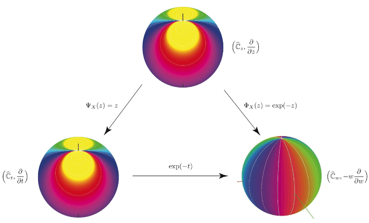
Figure 1. Diagram (3) for $X(z)=\frac{\partial}{\partial z}$. The holomorphic vector fields $\frac{\partial}{\partial z}$ and $-w\frac{\partial}{\partial w}$ on the Riemann sphere appear in a very natural context.

From these examples the case of pullbacks of $\frac{\partial}{\partial t}$ and $t\frac{\partial}{\partial t}$ (or $\pm w\frac{\partial}{\partial w}$) should be relevant, as we will conclude in §4.4.3.

Example 2 (Vector fields having maximal domain of their flows different from ${\mathbb{C}}_{t}$).

Let

$\big{(}{\widehat{\mathbb{C}}},X(z)=\frac{1}{R^{\prime}(z)}\frac{\partial}{\partial z}\big{)}$

be a rational vector field, for $R(z)$ a rational function of degree at least two. $X$ has at least one pole and note that the holomorphic differential equations theory can not be applied. However, in accordance with Diagram (12),

$\Psi_{X}(z)=R(z):{\widehat{\mathbb{C}}}_{z}\longrightarrow{\mathbb{C}}_{t}$

is single valued. Thus, $\pi_{X,1}$ provides a single valued global flow of $X$, with the property that

(13) $$R(z_{2})-R(z_{1})=\int\limits_{z_{1}}^{z_{2}}\omega_{X}=\begin{cases}\text{complex time to travel from }z_{1}\text{ to }z_{2}\\ \text{under the flow of }X,\end{cases}$$

for $z_{1},z_{2}\in{\widehat{\mathbb{C}}}$. In particular for $z_{1}$ a cero and $z_{2}\in{\widehat{\mathbb{C}}}\backslash Sing(X)$ the complex time $\infty$ makes sense. Moreover,

${\mathcal{R}}_{X}=\Omega_{X}=\{(z,R(z))\ |\ z\in{\widehat{\mathbb{C}}}\}.$

For further discussion see §12.

3.4. The singular complex analytic dictionary

Definition 2.

([10], p. 579) Let $\Psi:M\to{\mathbb{C}}$ be a singular complex analytic possibly multivalued function with a non–dense countable singular set $\overline{\mathcal{A}}$ such that the restriction of $\Psi$ to $M\backslash\overline{\mathcal{A}}$ is holomorphic. $\Psi$ is called additively automorphic if given two branches one has $\Psi_{\alpha}(z)=\Psi_{\beta}(z)+a_{\alpha\beta}$, for some constants $a_{\alpha\beta}\in{\mathbb{C}}$.

Note that $\Psi$ is single valued if and only if $a_{\alpha\beta}=0$ for all $\alpha,\beta$. However, the 1–form $d\Psi$ is always single valued on $M$, when Definition 2 holds true. For instance $\log(z)$ and $\log(P(z))$, for $P(z)$ a polynomial, are additively automorphic, however $P(z)\log(z)$ is not.

In summary one has the following result.

Proposition 1 (Singular complex analytic dictionary).

On any Riemann surface $M$ there is a canonical one–to–one correspondence between:

1. Singular complex analytic vector fields $X(z)=f(z)\frac{\partial}{\partial z}$.

2. Singular complex analytic differential forms $\omega_{X}$, related to $X$ via $\omega_{X}=\frac{dz}{f(z)}$.

3. Singular complex analytic orientable quadratic differential forms given by $\omega_{X}\otimes\omega_{X}$.

4. Singular (real) analytic flat structures $g_{X}$, satisfying $g_{X}(X)\equiv 1$, with suitable singularities on a non–dense countable set $\mathcal{A}\subset M$, trivial holonomy in $M\backslash\mathcal{A}$ and a (real) geodesible unitary vector field $W_{X}$ whose singularities are exactly $\mathcal{A}$.

5. Singular complex analytic (possibly multivalued) maps, distinguished parameters,

   $$\Psi_{X}(z)=\int^{z}_{z_{0}}\omega_{X}:M^{\diamond}\to{\widehat{\mathbb{C}}}$$

   where $z_{0}\in M^{\prime}$ and $z\in M^{\diamond}$.

6. Singular complex analytic (possibly multivalued) Newton maps

   $$\Phi_{X}(z)=\exp\left[-\int^{z}_{z_{0}}\omega_{X}\right]:M^{\diamond}\to{\widehat{\mathbb{C}}}$$

   where $z_{0}\in M^{\prime}$ and $z\in M^{\diamond}$.

7. The pairs $\big{(}{\mathcal{R}}_{X},\pi^{*}_{X,2}(\frac{\partial}{\partial t})\big{)}$ consisting of branched Riemann surfaces ${\mathcal{R}}_{X}$, associated to the maps $\Psi_{X}$, and the vector fields $\pi^{*}_{X,2}(\frac{\partial}{\partial t})$ under the projection $\pi_{X,2}:{\mathcal{R}}_{X}\longrightarrow{\widehat{\mathbb{C}}}_{t}$.

8. The pairs $(\Omega_{X},\mathcal{F})$ consisting of maximal domains $\Omega_{X}\subset M\times{\widehat{\mathbb{C}}}$ of the complex flows of $X$ and holomorphic foliations $\mathcal{F}$ whose leaves are copies of the Riemann surfaces ${\mathcal{R}}_{X}$.

Sketch of proof.

The equivalence between (1), (2) and (3) is well known and extensively used; it is only necessary to verify that the local complex analytic tensors transform in the required way, see §3.2.1 and §3.2.2.

That (4) follows from (3) uses the flat metric associated to $\omega_{X}\otimes\omega_{X}$, see §3.2.3.

For the converse assertion, we start with a flat structure $g$ on $M\backslash\mathcal{A}$. Since the riemannian holonomy of $g$, $\pi_{1}(M\backslash\mathcal{A})\longrightarrow O(2)$, is the identity, we recognize $W_{X}$ and its counterclockwise $\pi/2$ rotated vector field, say ${\text{\myfont e}}^{i\pi/2}W_{X}$, as the real and imaginary parts of a holomorphic vector field $X$ on $(M\backslash\mathcal{A},g)$. The extension of $X$ to $\mathcal{A}$ depends on the nature of the singularities of $X$. The suitable singularities hypothesis in (5), means that the extension exists. Obviously, poles and zeros of $X$ at $\mathcal{A}$ are suitable singularities and can be recognized by their normal forms in punctured neighborhoods, see Proposition 2. For further details see [5] lemma 2.6 and theorem D.

The equivalence between (5) and (6) and their relationship is further explored in §4.4.3. The correspondence between (5) and (7) follows from Diagram (12). Equivalence between (7) and (1) is postponed to §12, see Corollary 4. The same is true for the equivalence between (7) and (8): this is the content of Theorem 3 in §12. ∎

Remark 3.

Some comments are in order:

1. $\Psi_{X}$ and $\Phi_{X}$ as in (5) and (6) of Proposition 1 are well defined and holomorphic maps for $z$ at the poles of $\omega_{X}$.

2. The local map $\Psi_{\tt j}=\int d\zeta/f_{\tt j}(\zeta)$ in (7) is called distinguished parameter by K. Strebel [70] p. 20 and also by L. V. Ahlfors [1], we will continue using this name for the global map $\Psi_{X}$ described in (5) of Lemma 1.

3. The choice of initial and end points $z_{0},z$ for the integral defining $\Psi_{X}$ and $\Phi_{X}$ can be relaxed to include the essential singularities by integrating along asymptotic paths associated to asymptotic values of $\Psi_{X}$ at the essential singularities $E\subset M$, see remark 1.1 of [6].

4. Pullback of singular complex analytic vector fields

We start by recalling the classical local notion of holomorphically equivalent or conformally conjugated vector fields, see [17], [38] p. 9 for the usual concepts. Moreover, the following remains valid for regular points and singularities in the sense of Definition 1 (namely zeros, poles, isolated essential singularities of $X$ and accumulation points of the above at the origin).

Definition 3.

Let $X(z)=f(z)\frac{\partial}{\partial z}$ and $Y(z)=g(z)\frac{\partial}{\partial z}$ be two germs of singular complex analytic vector fields on $({\mathbb{C}}_{z},0)$ and let

$\varphi_{f}(z,t)$, $\varphi_{g}(z,t):\big{(}{\mathbb{C}}^{2}_{z\,t},(z_{0},0)\big{)}\longrightarrow({\mathbb{C}}_{z},0)$,

for a point $z_{0}$ where $f$ and $g$ are holomorphic, be their local holomorphic flows.

1. $X$ and $Y$ are topologically equivalent if there exists an orientation preserving homeomorphism $\Upsilon:({\mathbb{C}},0)\longrightarrow({\mathbb{C}},0)$ which takes trajectories of ${\mathfrak{Re}\left(X\right)}$ to trajectories of ${\mathfrak{Re}\left(Y\right)}$ preserving their orientation but not necessarily the parametrization.

2. $X$ and $Y$ are holomorphically equivalent if there exists a biholomorphism $\Upsilon:({\mathbb{C}},0)\to({\mathbb{C}},0)$ such that

   (14) $$\Upsilon(\varphi_{f}(z,t))=\varphi_{g}(\Upsilon(z),t)$$

   whenever both sides are well defined, for the maximal analytic continuations.

Note that, under the assumption that $\Upsilon$ is a biholomorphism, (14) is equivalent to $X=\Upsilon^{*}Y$.

Lemma 1.

Two germs of singular complex analytic vector fields $X(z)=f(z)\frac{\partial}{\partial z}$ and $Y(z)=g(z)\frac{\partial}{\partial z}$ on $({\mathbb{C}},0)$ are holomorphically equivalent if and only if there exists a biholomorphism $\Upsilon:({\mathbb{C}},0)\to({\mathbb{C}},0)$ such that

(15) $$f(z)=\frac{g(\Upsilon(z))}{\Upsilon^{\prime}(z)},\ \ \ \text{ for all }z\in({\mathbb{C}},0),\ \ \ z\neq 0.$$

Proof.

The proof follows by taking the derivative with respect to $t$ in (14). ∎

From a global point of view, two singular complex analytic vector fields $(M,X)$, $(N,Y)$ on arbitrary Riemann surfaces are holomorphically equivalent if there exists a biholomorphic map $\Upsilon:M\to N$ such that $\Upsilon(\varphi_{X}(z,t))=\varphi_{Y}(\Upsilon(z),t)$ whenever both sides are well defined.

4.1. Pullbacks of singular complex analytic vector fields by singular complex analytic maps

The pullback $\Upsilon^{*}$ is a natural operation when considering vector fields.

Lemma 2.

1. Given a singular complex analytic vector field $Y(t)=\Big{\{}g_{\tt k}(t)\frac{\partial}{\partial t}\Big{\}}$ on $N$ and a non–constant, singular complex analytic map

$$\Upsilon:M\rightarrow N,$$

the pullback vector field $X=\Upsilon^{*}Y=\Big{\{}f_{\tt j}(z)\frac{\partial}{\partial z}\Big{\}}$ is a singular complex analytic vector field well defined on $M$. In particular

(16) $$f_{\tt j}(z_{\tt j})=\frac{g_{\tt k}(\Upsilon_{\tt jk}(z_{\tt j}))}{\Upsilon^{\prime}_{\tt jk}(z_{\tt j})},$$

where $\Upsilon_{\tt jk}=\phi_{\tt jk}\circ\Upsilon\circ\phi_{\tt j}^{-1}$, $\Upsilon^{\prime}_{\tt jk}=\frac{d\Upsilon_{\tt jk}}{dz}$, and $\{\phi_{\tt j}:V_{\tt j}\subset M\rightarrow{\mathbb{C}}\}$, $\{\phi_{\tt k}:U_{\tt k}\subset N\rightarrow{\mathbb{C}}\}$ are the charts of $M$ and $N$ respectively.

2. Conversely, if $X$, $Y$ are given singular complex analytic vector fields on $M$, $N$ respectively and $\Upsilon$ is a (possibly multivalued) singular complex analytic function that satisfies (16), then

$$X=\Upsilon^{*}Y.$$

Proof.

Follows from Lemma 1 and an easy computation in local coordinates. ∎

The second statement concerning multivalued functions will be used in our work in §4.4.1 and §4.4.2.

We make a further convention: since we will be working on the Riemann surface $M$, no mention will be made of the local coordinates if these are not needed.

4.2. Normal forms

Clearly special attention is needed in the neighborhoods of singularities of the vector field $X$. Recall the description of the associated real flow and the normal forms for vector fields, see Figure 2. Several authors have contributed with proofs, see J. A. Jenkins [42] ch. 3, J. Gregor [30], [31], L. V. Ahlfors [1] p. 111, L. Brickman et al. [17], K. Strebel [70] ch. III, A. Garijo et al. [27]. Further discussion on the origin of normal forms can be found in [33], [5] pp. 133, 159, and references therein.

Proposition 2.

Let $X$ be a meromorphic vector field germ on $({\mathbb{C}},0)$ having a pole or zero at the origin. Up to local biholomorphism $X$ is holomorphically equivalent to one of the following normal forms.

1) For a pole of order $-\kappa\leq-1$

$$\frac{1}{z^{\kappa}}\frac{\partial}{\partial z}.$$

2) For simple zero

$$\frac{z}{\lambda}\frac{\partial}{\partial z},\ \ \ \lambda=Res(\omega_{X},0).$$

3) For zero of order $s\geq 2$

$$\frac{z^{s}}{1+\lambda z^{s-1}}\frac{\partial}{\partial z},\ \ \ \lambda=Res(\omega_{X},0).$$

$\Box$

In the case of functions the normal forms are simpler.

Lemma 3.

Let $g$ be a meromorphic function germ on $({\mathbb{C}},0)$ having a pole, regular point or zero at the origin. Up to local biholomorphism $g$ is equivalent to the following normal form

$z^{k}$     for $k\in{\mathbb{Z}}$ the multiplicity of $f$ at $0$.

$\Box$

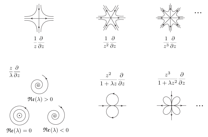
Figure 2. Phase portrait and normal forms of $X$ at a pole or zero. Top row: for a pole of order $-\kappa\leq-1$, the phase portrait has $2(\kappa+1)$ separatrices arriving or leaving the pole. Bottom row: simple zeros and zeros of order $s\geq 2$, here $\lambda=Res(\omega_{X},0)$. For simple zeros, the phase portrait is the pullback via $\Psi_{X}(z)=\lambda\log z$ of the constant vector field $Y(t)=\frac{\partial}{\partial t}$. For $s\geq 2$ the trajectories of $X$ form a flower with exactly $2(s-1)$ petals. For further details see Examples 1, 4, 5, and 6.

4.3. Geometry and dynamics of the pullback

Recall that a covering $\Psi:V\to W$ is a continuous surjective mapping such that for all $w\in W$, there exists an open set $U\ni w$ in $W$ with the characteristic that $\Psi^{-1}(U)$ is a disjoint union of open sets $O\subset V$ each of which satisfies that $\Psi:O\to U$ is a homeomorphism.

A branched or ramified covering $\Psi:V\to W$ is a covering except at a finite number of points of $W$. Said points are known as branch points or ramification points.

Remark 4 (Geometrical interpretation of the pullback).

In the setting of Lemma 2, it is now natural to consider singular complex analytic maps $\Upsilon:M\longrightarrow N$ as singular complex analytic ramified covering maps, thus providing a geometric interpretation of the pullback:

The trajectories of $X=\Upsilon^{*}Y$ are the pre–images, via $\Upsilon$ of the trajectories of $Y$.

Considering biholomorphisms as the covering maps we obtain:

Example 3 (A $PSL(2,{\mathbb{C}})$–action on vector fields).

Let $Y(t)=g(t)\frac{\partial}{\partial t}$ be a complex vector field on ${\widehat{\mathbb{C}}}_{t}$ and consider the pullback via a biholomorphism, $T(z)=\frac{az+b}{cz+d}$ with $ad-bc\neq 0$, of ${\widehat{\mathbb{C}}}$. Then

$$T^{*}\big{(}Y(t)\big{)}(z)=\frac{(cz+d)^{2}}{(ad-bc)}g(T(z))\frac{\partial}{\partial z}.$$

A useful particular case is when $T(z)=(1/z)$, so that $(T^{*}Y)(z)=-z^{2}g\left(1/z\right)\frac{\partial}{\partial z}$.

Considering finitely ramified coverings, we unify several known examples, poles are the simplest.

Example 4 (Poles of order $-\kappa\leq-1$).

The vector field

$X(z)=\frac{1}{z^{\kappa}}\frac{\partial}{\partial z}$   on $({\mathbb{C}},0)$,

has a pole of order $-\kappa$ at the origin. The natural diagram is

$X(z)$ is the pullback via the distinguished polynomial parameter

$\Psi_{X}(z)=\int^{z}\zeta^{\kappa}\,d\zeta=\frac{z^{\kappa+1}}{\kappa+1}$

of the constant vector field $Y(t)=\frac{\partial}{\partial t}$. The $2(\kappa+1)$ separatrices arrive or leave the pole in finite real time. See top row of Figure 2 and Figure 3 (a).

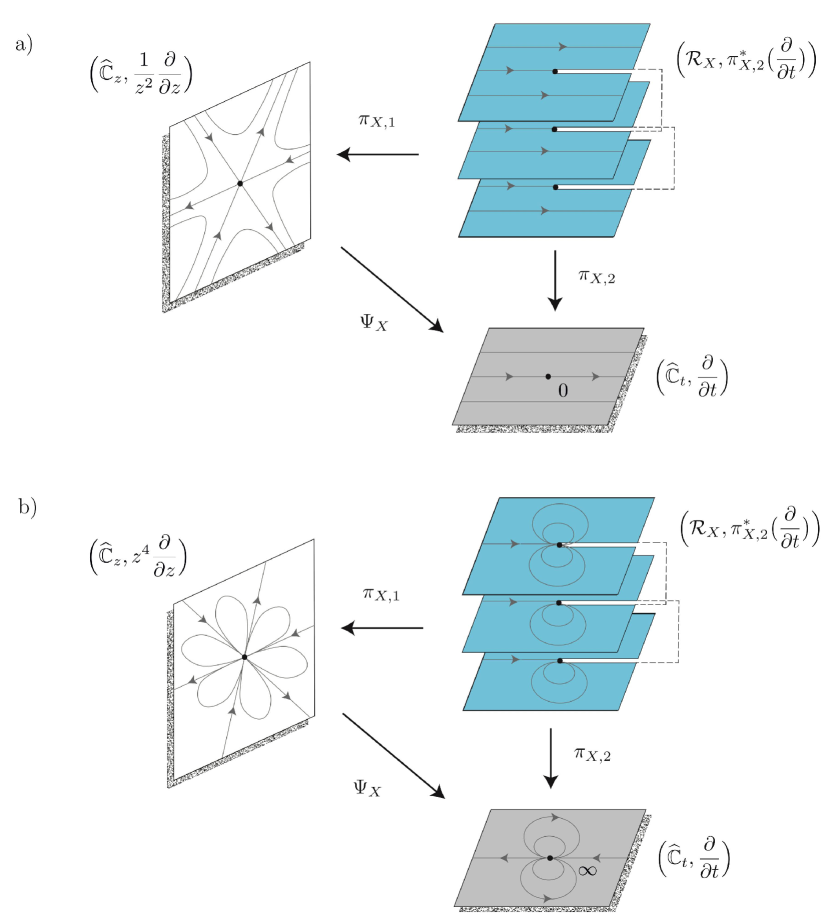
Figure 3. The diagrams for the Riemann surfaces ${\mathcal{R}}_{X}$ corresponding to $\frac{1}{z^{2}}\frac{\partial}{\partial z}$ and $z^{4}\frac{\partial}{\partial z}$.

Allowing $\log(z)$ as a ramified covering we obtain zeros.

Example 5 (Simple zeros $s=1$).

The vector field

$X(z)=\frac{1}{\lambda}z\frac{\partial}{\partial z}$   on ${\mathbb{C}}$, $\lambda\in{\mathbb{C}}^{*}$,

has a simple zero at the origin. The natural diagram is

$X(z)$ is the pullback via the distinguished additively automorphic parameter

$\Psi_{X}(z)=\int^{z}_{1}\frac{\lambda}{\zeta}\,d\zeta=\lambda\log(z)$

of the constant vector field $Y(t)=\frac{\partial}{\partial t}$. See bottom left of Figure 2.

Example 6 (Multiple zeros $s\geq 2$, with residue $\lambda\in{\mathbb{C}}$).

The vector field

$X(z)=\frac{z^{s}}{1+\lambda z^{s-1}}\frac{\partial}{\partial z}$,   $\lambda\in{\mathbb{C}}$,

has a zero or order $s\geq 2$ at the origin, and residue $\lambda$. The natural diagram is

$X(z)$ is the pullback of via the distinguished additively automorphic parameter

$\Psi_{X}(z)=\int^{z}_{1}\big{(}\frac{1}{\zeta^{s}}+\frac{\lambda}{\zeta}\big{)}\,d\zeta=\frac{1}{(1-s)z^{s-1}}+\lambda\log(z)-\frac{1}{1-s}$

of the constant vector field $Y(t)=\frac{\partial}{\partial t}$. See Figure 2 and Figure 3 (b).

Considering infinitely ramified covering maps we obtain essential singularities.

Example 7 (Essential singularity).

The entire vector field $X(z)={\text{\myfont e}}^{z}\frac{\partial}{\partial z}$ has an essential singularity at $\infty\in{\widehat{\mathbb{C}}}$ and no zeros or poles on ${\mathbb{C}}$. It is the pullback via the $\infty$ to $1$ ramified covering, $\Psi_{X}(z)=-{\text{\myfont e}}^{-z}$, of the constant vector field $\frac{\partial}{\partial t}$. It is considered to be the simplest example of an essential singularity. See Figure 4.

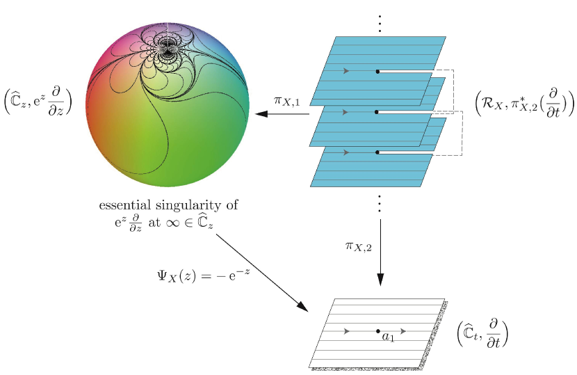
Figure 4. The diagram for a Riemann surface ${\mathcal{R}}_{X}$ corresponding to ${\text{\myfont e}}^{z}\frac{\partial}{\partial z}$.

4.4. Every singular complex analytic vector field is the pullback of $\frac{\partial}{\partial t}$ and of $-w\frac{\partial}{\partial w}$

4.4.1. Every singular complex analytic vector field admits a global flow box

A rather surprising result is the following, first presented in [5].

Theorem 4 (Pullbacks of $\frac{\partial}{\partial t}$).

Every singular complex analytic vector field $X$ on $M$ is the pullback of $\frac{\partial}{\partial t}$ on ${\widehat{\mathbb{C}}}_{t}$ via an additively automorphic singular complex analytic map $\Psi_{X}:M\longrightarrow{\widehat{\mathbb{C}}}_{t}$, i.e.

$${\Psi_{X}}_{*}X=\frac{\partial}{\partial t}.$$

Moreover

(17) $$\Psi_{X}(z)=\int_{z_{0}}^{z}\omega_{X},$$

for $z_{0}\in M^{\prime}$, and is a single–valued singular complex analytic function if and only if the periods and residues of $\omega_{X}$ are zero, i.e.

(18) $$\int_{\gamma}\omega_{X}=0\ \ \ \ \text{ for every}\ \ [\gamma]\in H_{1}(M^{\prime},{\mathbb{Z}}).$$

∎

Note that (18) implies that the zeros of $X$, if there are any, are of order $\geq 2$ (i.e. the poles of $\omega_{X}$ are non–simple). It also says that in this case $\omega_{X}$ is an exact differential 1–form.

The above result is of particular interest from the point of view of the theory of differential equations. Explicitly, the trajectories of $X$ are mapped to trajectories of $\frac{\partial}{\partial t}$, which are horizontal straight lines in ${\mathbb{C}}$ (recall that we speak of real trajectories as in (1)). This is a remarkable property: the existence and uniqueness of trajectories for singular complex analytic vector fields admits a very simple proof, that is also global on Riemann surfaces $M$. Recall that for real analytic vector fields, in general we can only obtain “long flow boxes”, see [61] ch. 3 §1. Moreover, $X$ does not present limit cycles, see [49], [9], [66]. Note that the point $z_{0}$ can be a pole of $X$ and the fact remains that ${\Psi_{X}}_{*}X=\frac{\partial}{\partial t}$ provides a flow box around $z_{0}$, as in Example 4.

4.4.2. Every singular complex analytic vector field is a pullback of $\lambda w\frac{\partial}{\partial w}$

Analogously one has the following result, also first presented in [5].

Theorem 5 (Pullbacks of $\frac{1}{\lambda}w\frac{\partial}{\partial w}$).

Every singular complex analytic vector field $X$ on $M$ is the pullback of $\frac{1}{\lambda}w\frac{\partial}{\partial w}$ on ${\widehat{\mathbb{C}}}_{w}$, for any $\lambda\in{\mathbb{C}}^{*}$, via a (possibly multivalued) singular complex analytic map $\Phi_{X}(z):M\longrightarrow{\widehat{\mathbb{C}}}_{w}$, i.e.

$${\Phi_{X}}_{*}\big{(}X\big{)}(w)=\frac{1}{\lambda}w\frac{\partial}{\partial w}.$$

Moreover

(19) $$\Phi_{X}(z)=\exp\Big{(}\frac{1}{\lambda}\int_{z_{0}}^{z}\omega_{X}\Big{)},$$

for $z_{0}\in M^{\prime}$, and is a single–valued singular complex analytic function if and only if the periods and residues of $\omega_{X}$ are integer multiples of some complex number $\Pi\in{\mathbb{C}}^{*}$, i.e.

(20) $$n\Pi=\int_{\gamma}\omega_{X}\ \ \ {\it for\ [\gamma]\in H_{1}(M^{\prime},{\mathbb{Z}})},\ \ n\in{\mathbb{Z}}\ .$$

Proof.

By Lemma 2, $X(z)$ is the pullback of $\frac{1}{\lambda}w\frac{\partial}{\partial w}$ iff

$$f(z)=\frac{1}{\lambda}\frac{\Phi_{X}(z)}{\Phi_{X}^{\prime}(z)},$$

for some (possibly multivalued) singular complex analytic function $\Phi_{X}$ on $M$. Equivalently $1/(\lambda f(z))$ is the logarithmic derivative of $\Phi_{X}(z)$, hence upon integration and exponentiation one obtains the expression (19) for $\Phi_{X}$.
On the other hand, by virtue of the explicit form of $\Phi_{X}$ and since $\exp$ is $2\pi i$–periodic, the differential form $\omega_{X}$ has a residue or period that is not an integer multiple of $\Pi=2\pi i\lambda$ if and only if $\Phi_{X}(z)$ is multivalued. ∎

4.4.3. Correspondence between $\frac{\partial}{\partial t}$ and $-w\frac{\partial}{\partial w}$

As was seen in the previous two sections, one can express any singular complex analytic vector field $X$ on $M$ as the pullback of either $\frac{\partial}{\partial t}$ or $-w\frac{\partial}{\partial w}$ via the (possibly multivalued) functions

$$\Psi_{X}(z)=\int_{z_{0}}^{z}\omega_{X}\qquad\text{ and }\qquad\Phi_{X}(z)=\exp\Big{(}-\int_{z_{0}}^{z}\omega_{X}\Big{)},$$

respectively.

Corollary 1.

Let $X$ be a singular complex analytic vector field on $M$. It is the pullback of $\frac{\partial}{\partial t}$ and it is also the pullback of $-w\frac{\partial}{\partial w}$. Furthermore $\frac{\partial}{\partial t}$ is the pullback via $\exp(-t)$ of $-w\frac{\partial}{\partial w}$ and we have the following commutative diagram

for the respective (possibly multivalued) singular complex analytic functions. ∎

Corollary 1 is exemplified in Figure 5 for the entire vector field $X(z)=-{\text{\myfont e}}^{-z{\text{\myfont e}}^{z}}\frac{\partial}{\partial z}$ which has a class 2 essential singularity at $\infty\in{\widehat{\mathbb{C}}}$, see [5]. Yet it is the pullback of both $\frac{\partial}{\partial t}$ and $-w\frac{\partial}{\partial w}$.

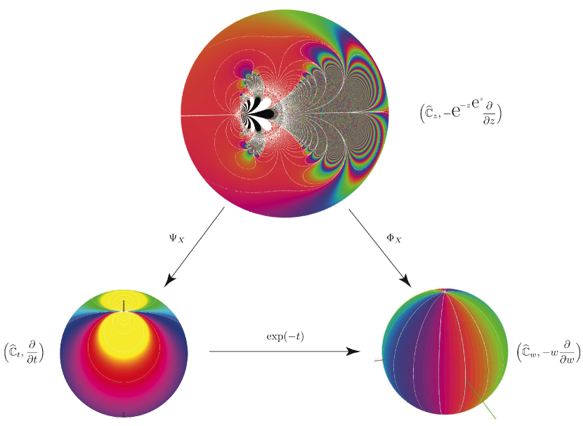
Figure 5. Example of Diagram 3 for $X(z)=-{\text{\myfont e}}^{-z\,{\text{\myfont e}}^{z}}\frac{\partial}{\partial z}$.

5. Newton vector fields: pullbacks of $-w\frac{\partial}{\partial w}$

We now recall a special kind of complex analytic vector fields that were first studied in the 80’s, by M. W. Hirsch, S. Smale and M. Shub ([35], [69], [68], [21]). The concept of Newton vector field was introduced together with that of Newton graphs that arise from studying Newton’s method of root finding for a complex polynomial. Taking their definition as a guide we have:

Definition 4.

A singular complex analytic vector field $X(z)=f_{\tt j}(z)\frac{\partial}{\partial z}$ on $M$ is said to be a Newton vector field if it can be represented as

$$X(z)=-\frac{\Phi_{\tt j}(z)}{\Phi^{\prime}_{\tt j}(z)}\frac{\partial}{\partial z},$$

for some (possibly multivalued) singular complex analytic function $\{\Phi_{\tt j}\}$ on $M$.

From the definition and the results of §4.4.2 one has as an immediate consequence that $\Phi=\Phi_{X}$ and the following.

Corollary 2.

Every singular complex analytic vector field $X$ on an arbitrary Riemann surface $M$ is a Newton vector field of a suitable $\Phi_{X}$.

Example 8.

The complex vector field

$$X(z)=-\tan(z)\frac{\partial}{\partial z}$$

is the pullback via $\Phi_{X}(z)=\sin(z)$ of the complex vector field $Y(t)=-w\frac{\partial}{\partial w}$, so in fact it is a Newton vector field.

On the other hand, recalling the geometrical interpretation of the pullback, and considering $\Phi_{\alpha}:M_{z}\longrightarrow{\widehat{\mathbb{C}}}_{w},$ a singular complex analytic ramified covering over the sphere, one can construct Newton vector fields as the pullback via $\Phi_{\alpha}$ of the radial vector field $-w\frac{\partial}{\partial w}$ on the Riemann sphere. Note also that the composition of ramified coverings is still a ramified covering, hence:

Corollary 3.

Let $S_{w}$, $N_{t}$ and $M_{z}$ be Riemann surfaces and let $Y(w)=g(w)\frac{\partial}{\partial w}$ be a singular complex analytic vector field on $S_{w}$. Further suppose that

$$\Phi_{1}:M_{z}\longrightarrow N_{t},\quad\Phi_{2}:N_{t}\longrightarrow S_{w}$$

are singular complex analytic ramified coverings, then $X(z)=f(z)\frac{\partial}{\partial z}$ is the pullback via $\Phi=\Phi_{2}\circ\Phi_{1}$ of $Y(w)$ if and only if

$$f(z)=\frac{g(\Phi(z))}{\Phi^{\prime}(z)}=\frac{g(\Phi_{2}(\Phi_{1}(z)))}{\Phi_{2}^{\prime}(\Phi_{1}(z))\ \Phi_{1}^{\prime}(z)}.$$

Proof.

The proof is a direct consequence of the chain rule and Lemma 2. ∎

So by considering $Y(w)=-w\frac{\partial}{\partial w}$ we can construct many Newton vector fields. Some examples follow.

Example 9.

The complex vector field

$$X(z)=-(\cosh(z)+1)\frac{\partial}{\partial z}$$

is obtained from $-w\frac{\partial}{\partial w}$ via pullback with $\Phi_{X}=\Phi_{3}\circ\Phi_{2}\circ\Phi_{1}$, where $\Phi_{3}(s)={\text{\myfont e}}^{s}$, $\Phi_{2}(t)=\frac{t-1}{t+1}$ and $\Phi_{1}(z)={\text{\myfont e}}^{z}$. It has zeros at $z_{n}=i(2n+1)\pi,\ n\in{\mathbb{Z}}$.

Example 10.

The complex vector field

$$X(z)={\text{\myfont e}}^{z}\frac{\partial}{\partial z}$$

is obtained from $-t\frac{\partial}{\partial t}$ via pullback with $\Phi_{X}=\Phi_{2}\circ\Phi_{1}$, where $\Phi_{2}(w)={\text{\myfont e}}^{w}$ and $\Phi_{1}(z)={\text{\myfont e}}^{-z}$. It has an essential singularity at $\infty$.

Example 11.

The complex vector field

$$X(z)=\frac{{\text{\myfont e}}^{z^{3}}}{3z^{3}-1}\frac{\partial}{\partial z}$$

is obtained from $-w\frac{\partial}{\partial w}$ via pullback with $\Phi_{X}=\Phi_{2}\circ\Phi_{1}$, where $\Phi_{2}(w)=w{\text{\myfont e}}^{-w^{3}}$ and $\Phi_{1}(z)={\text{\myfont e}}^{-z}$. It has an essential singularity at $\infty$ and 3 poles on the finite plane.

Remark 5.

It should be noted that when $\Psi$ is rational, the $\omega$–limit set of almost any trajectory for the flow of

$X(z)=\frac{\Psi(z)}{\Psi^{\prime}(z)}\frac{\partial}{\partial z}$

on $M$ corresponds to the zeros of $\Psi$, in agreement with the work of M. W. Hirsch, S. Smale and M. Shub ([35], [69], [68], [21]).

However, when $\Psi$ is not rational, the $\omega$–limit could be an isolated essential singularity (Examples 10 and 11) or an accumulation point of poles or zeros (Examples 8 and 9).

In Table 1 we present a summary of the different objects and their relations, encountered so far. There we can observe that the residue of $\omega_{X}$ plays an important role in the description of the objects. This was already observed in [5], §5.7.

Table 1. Relationship between vector fields, 1–forms, distinguished parameter and the Newton covering map germs.

Complex analytic	Complex analytic	Distinguished	Newton
vector field	1–form	parameter	covering map
$X(z)=f(z)\frac{\partial}{\partial z}$	$\omega_{X}=\frac{dz}{f(z)}$	$\Psi_{X}(z)=\int\limits^{z}\omega_{X}$	$\Phi_{X}(z)={\text{\myfont e}}^{-\Psi_{X}(z)}$
pole of	zero of	zero of
order $-\kappa\leq-1$	order $\kappa$	order $\kappa+1$
$\frac{1}{z^{\kappa}}\frac{\partial}{\partial z}$	$z^{\kappa}\,dz$	$\frac{1}{\kappa+1}z^{\kappa+1}$	${\text{\myfont e}}^{-\frac{1}{\kappa+1}z^{\kappa+1}}$
simple zero	simple pole
$\frac{1}{\lambda}z\frac{\partial}{\partial z}$	$\frac{\lambda}{z}\,dz$	$\lambda\log(z)$	$z^{-\lambda}$
multiple zero $s\geq 2$	multiple pole
$\frac{z^{s}}{1+\lambda z^{s-1}}\frac{\partial}{\partial z}$	$\left(\frac{1}{z^{s}}+\frac{\lambda}{z}\right)dz$	$\Big{(}\frac{1}{(1-s)z^{s-1}}\hfill$	$z^{-\lambda}{\text{\myfont e}}^{(s-1)z^{s-1}}$
	$\lambda=Res(\omega_{X},0)$	$\hfill+\ \lambda\log(z)\Big{)}$
essential	essential
singularity at $\infty$	singularity at $\infty$
${\text{\myfont e}}^{P(z)}\frac{\partial}{\partial z}$	${\text{\myfont e}}^{-P(z)}dz$	$\int\limits^{z}{\text{\myfont e}}^{P(\zeta)}d\zeta$	${\text{\myfont e}}^{-\int\limits^{z}{\text{\myfont e}}^{P(\zeta)}d\zeta}$

6. Visualization of Newton vector fields

We now move on to describe the actual method that will enable us to solve for the trajectories of (and hence visualize) Newton vector fields. As mentioned in the introduction, the idea behind is that there are two auxiliary real valued functions: one whose level curves correspond to trajectories (streamlines) of the complex vector field (in differential equations this auxiliary function is called a first integral), and the other one which is linear along the trajectories, hence providing the parametrization of the solution.

6.1. The fundamental observation

Let

$$X(z)=f(z)\frac{\partial}{\partial z}=-\frac{\Phi_{X}(z)}{\Phi^{\prime}_{X}(z)}\frac{\partial}{\partial z}$$

be a Newton vector field, recall that the trajectories $z(\tau)$ are the solutions to

(21) $$\left\{\begin{aligned} z^{\prime}(\tau)&=-\frac{\Phi_{X}\big{(}z(\tau)\big{)}}{\Phi^{\prime}_{X}\big{(}z(\tau)\big{)}},\\ z(0)&=z_{0},\end{aligned}\right.$$

for $\tau\in{\mathbb{R}}$, as in (1).

Lemma 4 (Fundamental observation).

A trajectory $z(\tau)$ of $X$ satisfies

(22) $$\Phi_{X}\big{(}z(\tau)\big{)}=\Phi_{X}(z_{0}){\text{\myfont e}}^{-\tau}$$

if and only if $z(\tau)$ is a trajectory, passing through $z_{0}$, of the Newton vector field corresponding to $\Phi_{X}$.

Proof.

The proof follows from implicitly differentiating the equation

$$\Phi_{X}\big{(}z(\tau)\big{)}=\Phi_{X}(z_{0}){\text{\myfont e}}^{-\tau},$$

that is

$$\Phi^{\prime}_{X}\big{(}z(\tau)\big{)}z^{\prime}(\tau)=-\Phi_{X}(z_{0}){\text{\myfont e}}^{-\tau}$$

so that

$$z^{\prime}(\tau)=-\frac{\Phi_{X}\big{(}z(\tau)\big{)}}{\Phi^{\prime}_{X}\big{(}z(\tau)\big{)}},$$

hence $z(\tau)$ is indeed a solution to (21). ∎

The fundamental observation can be understood in terms of the pullback as follows: The trajectory $z(\tau)$ is the flow of the pullback, via $\Phi$, of the field $-w\frac{\partial}{\partial w}$ (whose trajectories are straight lines, parametrized by ${\text{\myfont e}}^{-\tau}$, that start at $\infty$ and end at $0$ in ${\widehat{\mathbb{C}}}_{t}$). See Figure 6.

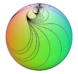
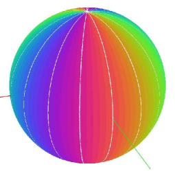
Figure 6. The trajectories $z(t)$ correspond to trajectories of $-w\frac{\partial}{\partial w}$ under the covering map $\Phi_{X}$.

Consider now the Newton vector field normal to $X$,

$$X^{\perp}(\zeta)=i\ f(\zeta)\frac{\partial}{\partial\zeta}=-\frac{{\widetilde{\Phi}_{X}}(\zeta)}{{\widetilde{\Phi}}^{\prime}_{X}(\zeta)}\frac{\partial}{\partial\zeta},$$

with ${\widetilde{\Phi}_{X}}$ being its corresponding covering map. Then one has

$$-i\left(\log\Phi_{X}\right)^{\prime}=-i\frac{\Phi^{\prime}_{X}}{\Phi_{X}}=\frac{{\widetilde{\Phi}}^{\prime}_{X}}{{\widetilde{\Phi}}_{X}}=\left(\log{\widetilde{\Phi}_{X}}\right)^{\prime},$$

and it follows that ${\widetilde{\Phi}_{X}}=\Phi^{-i}_{X}$. Thus taking $\log(z)$ on both sides we obtain that

(23) $$\rho(z)\doteq\log\left\lvert\widetilde{\Phi}_{X}(z)\right\rvert =\arg\left(\Phi_{X}(z)\right)$$

$$\theta(z)\doteq\arg\left({\widetilde{\Phi}}_{X}(z)\right) =-\log\left\lvert\Phi_{X}(z)\right\rvert.$$

Proposition 3 (Solving $\dot{z}=-\frac{\Phi_{X}(z)}{\Phi^{\prime}_{X}(z)}$).

Let $z(\tau)$ be a trajectory of a singular complex analytic field

$$X(z)=-\frac{\Phi_{X}(z)}{\Phi^{\prime}_{X}(z)}\frac{\partial}{\partial z},$$

then

1. $\arg\left(\Phi_{X}(z(\tau))\right)=\arg\left(\Phi_{X}(z_{0})\right)$ is constant along the trajectories $z(\tau)$ of $X$, and

2. $\log\left\lvert\Phi_{X}(z(\tau))\right\rvert=-\tau+\log\left\lvert\Phi_{X}(z_{0})\right\rvert$ is linear along the trajectories $z(\tau)$ of $X$,

where $z_{0}=z(0)$.

Proof.

For (1) use (23) and the fundamental observation (Lemma 4).

For (2), a similar argument works. ∎

As a direct consequence we can now state the main theorem related to the visualization of singular complex analytic vector fields.

Theorem 1 (Visualization of singular complex analytic vector fields).

Let $X(z)=f(z)\frac{\partial}{\partial z}$ be a singular complex analytic vector field on a Riemann surface $M$, and let $z(\tau)$ denote any trajectory of $X$ on $M\backslash Sing(X)$. Then there exist two (probably multivalued) functions $\rho,\theta:M\backslash Sing(X)\longrightarrow{\mathbb{R}}$ such that

1. The real valued function $\rho$ is constant along $z(\tau)$. Hence in order to visualize the trajectories that pass through the point $z_{0}\in M$, one needs only plot the level curve $\rho(z)=\rho(z_{0})$.

2. The real valued function $\theta$ defines a natural time parametrization along the trajectory $z(\tau)$. In other words, if $z(\tau)$ is the trajectory passing through $z_{0}$ at $\tau=0$, then the point $z(\tau_{1})$ is given by the intersection of the curves $\rho(z)=\rho(z_{0})$ and $\theta(z)=\theta(z_{0})+\tau_{1}$.

Moreover, $\rho$ and $\theta$ can be expressed in terms of the distinguished parameter $\Psi_{X}$ and the Newton map $\Phi_{X}$ as:

(24) $$\begin{array}[]{c}\rho(z)=\arg\left(\Phi_{X}(z)\right)=-{\mathfrak{Im}\left(\Psi_{X}(z)\right)},\\ \theta(z)=-\log\left\lvert\Phi_{X}(z)\right\rvert={\mathfrak{Re}\left(\Psi_{X}(z)\right)}.\end{array}$$

Proof.

(1) Is a direct consequence of Proposition 3.a where $\rho(z)=\arg\left(\Phi_{X}(z)\right)$.

(2) Follows directly from Proposition 3.b, i.e. the linear behaviour of $\theta(z)=\log\left\lvert\Phi_{X}(z)\right\rvert$ along the trajectory $z(\tau)$:

$\theta(z(\tau_{1}))=-\log\left\lvert\Phi_{X}(z(\tau_{1}))\right\rvert=-\log\left\lvert\Phi_{X}(z_{0})\right\rvert+\tau_{1},$

and from the description of the trajectory $z(\tau)$:

$\rho(z(\tau_{1}))=\rho(z_{0}).$

Finally, Corollary 1, particularly Diagram 3, shows that $\rho$ and $\theta$ can be expressed in terms of $\Psi_{X}$ or $\Phi_{X}$ so (24) follows. ∎

Remark 6.

1. The auxiliary functions $\rho$ and $\theta$ are known as constants of motion, integrals of motion, or first integrals. On the other hand, recall that a generic real analytic vector field does not have a first integral.

2. The acute reader will note that $\rho$ and $\theta$ determine visualizations of the functions $\Phi_{X}$ and $\Psi_{X}$ as polar and rectangular representations respectively.

This last remark provides a counterpart for Theorem 1

Theorem 2 (Visualization of singular complex analytic functions).

1. Let $\Psi:M\longrightarrow{\widehat{\mathbb{C}}}$ be a singular complex analytic function. Then the phase portraits of

   $X(z)=\frac{1}{\Psi^{\prime}(z)}\frac{\partial}{\partial z}$  provides the level curves of $-{\mathfrak{Im}\left(\Psi\right)}$,

   $X^{\perp}(z)\doteq\frac{i}{\Psi^{\prime}(z)}\frac{\partial}{\partial z}$  provides the level curves of ${\mathfrak{Re}\left(\Psi\right)}$.

2. Let $\Phi:M\longrightarrow{\widehat{\mathbb{C}}}$ be a singular complex analytic function. Then the phase portraits of

   $X(z)=-\frac{\Phi(z)}{\Phi^{\prime}(z)}\frac{\partial}{\partial z}$  provides the level curves of $\arg\left(\Phi\right)$,

   $X^{\perp}(z)\doteq-i\frac{\Phi(z)}{\Phi^{\prime}(z)}\frac{\partial}{\partial z}$  provides the level curves of $-\log{\left\lvert\Phi\right\rvert}$.

∎

Remark 7 (Solution for the flow of $X$ and no propagation of error along the trajectories of $X$).

The above theorem shows that we are not only visualizing the flow of the singular complex analytic vector field, but we are in fact

completely solving the system of differential equations that define the flow

including parametrization of the singular complex analytic vector field $X(z)$.

Contrast this with the usual visualization techniques where information relating to the parametrization is not observed.

Moreover, the solutions are exact up to the numerical round–off errors incurred by the precision of the mathematical routines used in the implementation. In other words, there is no error propagated along the trajectories of $X$.

6.2. The algorithms

Given a singular complex analytic vector field

$$X(z)=f(z)\frac{\partial}{\partial z}=-\frac{\Phi_{X}(z)}{\Phi^{\prime}_{X}(z)}\frac{\partial}{\partial z},$$

according to Theorem 1 and (24), we require the plotting of the level curves of the real valued function $\rho(z)=\arg\left(\Phi_{X}(z)\right)=-{\mathfrak{Im}\left(\Psi_{X}(z)\right)}$.

This can be done both on the (complex) plane and more generally on the Riemann surface $M$. Moreover, it will be convenient to plot strip flows, where, given an interval $[a,b)\subset{\mathbb{R}}$ we define the strip flow associated to $[a,b)$ as

(25) $$B_{[a,b)}=\big{\{}z\in M\ |\ \rho(z)\in[a,b)\big{\}}\subset M.$$

In this way the border is the level curves $\rho(z)=a$ and $\rho(z)=b$, which correspond to trajectories of the singular complex analytic vector field $X$. Note that $B_{[a,b)}$ can be a multiply connected subset of $M$.

In the following algorithm we present the case of $M$ being either the plane ${\mathbb{C}}$ or the Riemann sphere ${\widehat{\mathbb{C}}}$, the case of a general Riemann surface is similar and is further discussed in §10.

We can use strip flows to visualize the streamlines on the plane or Riemann sphere, using the following:

Visualization algorithm.

(p refers to the plane, s to the sphere.)

1. Partition ${\mathbb{R}}$ into intervals $\big{\{}[a_{\iota},b_{\iota})\big{\}}$ and select a color $C_{\iota}$ for each interval $[a_{\iota},b_{\iota})$ of the partition.

2. Choose a rectangular region of the plane (say $R=[x_{min},x_{max}]\times[y_{min},y_{max}]$) where the visualization is to take place, and a window size of say $N$ by $M$ pixels, then subdivide the rectangular region of the plane into $N\times M$ rectangular regions of size $\Delta x=(x_{max}-x_{min})/N$ by $\Delta y=(y_{max}-y_{min})/M$, note that each of these rectangular regions corresponds to a pixel on the window.

3. A triangulation of the Riemann sphere is constructed using a recursive algorithm that ensures that the triangulation is almost uniform (start with a octahedron with vertices on the sphere and recursively add a vertex at the center of each triangle and then normalize the vertex to obtain a better triangulation for the sphere, consult [13] for more details).

4. For each rectangle of the subdivision of $R$ (a pixel) calculate its center $z\in R\subset{\mathbb{C}}$.

5. For each triangle in the triangulation of the sphere, one finds the barycentre $z^{*}$ and using stereographic projection we identify the corresponding $z\in{\mathbb{C}}$.

6. We proceed to calculate $\rho(z)$ (or $\rho(z^{*})$).

7. Since ${\mathbb{R}}$ is partitioned into intervals $\rho(z)\in[a_{\iota},b_{\iota})$ for some $\iota$, we proceed to color the pixels (triangles), on the plane (Riemann sphere), corresponding to $z$ (or $z^{*}$) with the color $C_{\iota}$.

Remark 8.

Note that steps (2p) and (2s) ensure that both the resolution on the rectangular region $R$ of the plane and on the Riemann sphere, are uniform.

6.2.1. Plotting specific level curves

Due to the fact that there are an infinite number of trajectories intersecting a given zero, it is very easy to identify the zeros of the corresponding Newton vector field.

However the actual position of the poles are not so easily identified: by the nature of the poles (recall Proposition 2 and Example 4), a pole of order $-\kappa\leq-1$ has exactly $(2\kappa+2)$ separatrices.

Similarly, it was shown in [5] definition 4.11, that for essential singularities there exists trajectories that are analogs of the separatrices of poles: the horizontal asymptotic paths that have as $\alpha$ or $\omega$ limit set the essential singularity.

With the above in mind and recalling that singular complex analytic vector fields on ${\widehat{\mathbb{C}}}$ can not have limit cycles, we then can make the following observation.

Remark 9 (Plotting separatrices and horizontal asymptotic paths).

In order to correctly visualize the phase portrait of singular complex analytic vector fields, it is convenient to plot

$\bullet$ the separatrices of a pole and

$\bullet$ the horizontal asymptotic paths for essential singularities,

i.e. specific trajectories of the field (that is specific level curves of the real valued function $\rho$).

Recall the classical ideas of L. Markus and H. Benzinger on the decomposition of the phase portraits using the above kind of specific trajectories, [53], [9], more recently [16], [5] §11.

Suppose we want to plot a specific trajectory, say one that passes through or has $\alpha$ or $\omega$ limit set a point $z_{0}$ on the plane. Then by Theorem 1 we need to plot the level curve of $\rho$ corresponding to the value $\rho_{0}=\rho(z_{0})$. Since the fundamental unit we are using for the visualization is the subdivision by rectangles on the rectangle $R\subset{\mathbb{C}}$ (or the triangulation of the Riemann sphere ${\widehat{\mathbb{C}}}$), we need to color those rectangles (or triangles) that intersect the level curve. For this note that

• the function $\widehat{\rho}(z,z_{0})=\rho(z)-\rho(z_{0})$ can be zero in the interior of a rectangle (triangle), even though at the center (or barycentre) it could be different from zero,

• we only want to color rectangles (or triangles) that intersect the level curve $\widehat{\rho}(z,z_{0})=0$.

To achieve this we have the following:

Visualization algorithm for specific level curves.

1. Once again we find the center $z$ of each rectangle (or the barycentre $z^{*}$ of each triangle), as well as the maximum distance $\delta$ from the center (or barycentre) to each of the vertices. Note that in the case of the plane, $\delta=\sqrt{{\Delta x}^{2}+{\Delta y}^{2}}$, since the basic unit is a rectangle.

2. Using the fact that the gradient of a real valued function points in the direction of maximum growth, let $\hat{e}=\frac{\nabla\widehat{\rho}(z,z_{0})}{\left\lvert\nabla\widehat{\rho}(z,z_{0})\right\rvert}=\frac{\nabla\rho(z)}{\left\lvert\nabla\rho(z)\right\rvert}$ be the unit vector that points in the direction of maximum growth of $\widehat{\rho}(\cdot,z_{0})$ at $z$ (or $z^{*}$). Note that $\widehat{\rho}(\cdot,z_{0})$ is a $C^{\infty}$ function since it is the real part of an analytic function. In fact, $\hat{e}=\frac{X^{\perp}(z)}{\left\lvert X^{\perp}(z)\right\rvert}$ $\left(\text{or }\hat{e}=\frac{X^{\perp}(z^{*})}{\left\lvert X^{\perp}(^{*})\right\rvert}\right)$.

3. Recalling that the sign of $\widehat{\rho}$ changes if and only if $\widehat{\rho}$ assumes the value zero, we consider the product

   $$\widehat{\rho}(z+\delta\hat{e},z_{0})\ \widehat{\rho}(z-\delta\hat{e},z_{0}),$$

   and so the level curve $\widehat{\rho}=0$ intersects the rectangle (or triangle) if the above product is less than zero, so we color the rectangle (or triangle) associated to $z$ (or $z^{*}$) if this happens.

In this way those rectangles (or triangles) that intersect the level curve $\widehat{\rho}=0$ are colored.

Remark 10.

Note that the above algorithm:

1. Is optimal with respect to resolution for the case of the plane: that is one obtains the best possible observable resolution. If one would increase the size of the rectangular mesh $\Delta x\times\Delta y$ one would observe pixelation, and if one decreases the size of the rectangular mesh $\Delta x\times\Delta y$, then no gain in resolution would be observed, since the size of the rectangular mesh would be smaller that the size of each pixel on the screen.

2. Is not optimal for the case of the sphere: since in this case the actual observed resolution will depend on the particular parameters (viewpoint, distance of the camera to the sphere, etc.) used in the visualization of the sphere as a 3D object on the screen.

3. However, given a specific resolution, the algorithms ensure that no error is made as to which streamlines intersect the chosen basic rectangles (or triangles) that specify the resolution, hence for the chosen resolution the visualization is the best possible.

6.3. Parallelization of the visualization algorithms

It is clear that this method is a prime candidate for parallelization, due to the fact that the visualization scheme for a particular pixel does not depend on the neighboring pixels. Hence a simple parallelization scheme where blocks of pixels are assigned to distinct processors can be readily implemented. An extensive analysis and implementation of this is yet to be done and will be presented elsewhere.

7. Analytic recognition of the ramified covering $\Phi_{X}$

As was shown in the previous section, Newton vector fields benefit from the visualization scheme just presented, and since all singular complex analytic vector fields are Newton vector fields, this makes the visualization scheme presented much more appealing.

Of course one still has to be able to explicitly calculate the real valued functions $\rho(z)$ and $\theta(z)$ of Theorem 1 in order to make use of the method.

In this aspect, the first author et.al. shows in [4] that there is a large class of vector fields meromorphic on the plane, for which it is possible to explicitly construct the ramified covering $\Phi_{X}$ characterizing the vector field as a Newton vector field (and hence $\rho(z)$ and $\theta(z)$ of Theorem 1 can also be calculated explicitly). In the same work they show again by an explicit construction, that all doubly periodic (elliptic) vector fields (and hence vector fields on the torus) for which it is possible to analytically recognize the ramified covering $\Psi_{X}$ (see §10.1.2 for an example of an elliptic vector field).

We recall these results in this section. Let $\mathscr{F}$ be the family of functions that satisfy the requirements of Cauchy’s Theorem on Partial Fractions (see [4] for further details). Suppose that $g\in\mathscr{F}$, denote by

$$G_{k}(z)=\sum_{j=1}^{N_{k}}\frac{a_{jk}}{(z-b_{k})^{j}},$$

the principal part of $g(z)$ at the pole $b_{k}$ of order $N_{k}$; and let

$$P_{k}(z)=\sum_{j=0}^{p}\widetilde{a}_{jk}z^{j},$$

denote the corresponding polynomials (in case $p>-1$). Then in [4] it was proved that:

Theorem 6.

Let $f(z)\in\mathscr{F}$. Then there is a meromorphic (possibly multivalued) function

(26) $$\Phi_{X}(z)=\prod_{k=1}^{\infty}\left[(z-b_{k})^{-A_{k}}{\text{\myfont e}}^{q_{k}\left(\frac{1}{z-b_{k}}\right)}{\text{\myfont e}}^{Q_{k}(z)}\right],$$

where $q_{k}(z)$ and $Q_{k}(z)$ are unique polynomials with $q_{k}(0)=0$ and $Q_{k}(0)=0$, such that

$$f(z)=-\frac{\Phi_{X}^{\prime}(z)}{\Phi_{X}(z)}.$$

∎

As a quick, and illustrative, example of the explicit construction of the $\Phi_{X}$ defining the Newton vector field, we consider the case of rational functions: let

(27) $$f(z)=-\frac{p(z)}{q(z)}$$

with $q,p\in{\mathbb{C}}[z]$ without common factors, and $p$ monic. In particular consider

(28) $$p(z)=\prod_{j=1}^{J}(z-z_{j})^{m_{j}},\quad q(z)=b\prod_{k=1}^{K}(z-s_{k})^{n_{k}},$$

where $m_{j},n_{k}\in{\mathbb{Z}}$ and $b\in{\mathbb{C}}$ are constants.

We then obtain theorem 2.3 of [9] as a corollary of our Theorem 6 (for the particular case of rational functions):

Theorem 7 (H. E. Benzinger [9]).

$f(z)$ is a rational function as in (27) that satisfies

$$f(z)=-\frac{\Phi_{X}(z)}{\Phi_{X}^{\prime}(z)}$$

if and only if there exist unique polynomials $P_{j}$, with $P_{j}(0)=0$, and unique constants $A_{j}\in{\mathbb{C}}$, $j=1,\dots,J$, such that

(29) $$\Phi_{X}(z)=C{\text{\myfont e}}^{P_{0}(z)}\prod_{j=1}^{J}(z-z_{j})^{A_{j}}{\text{\myfont e}}^{P_{j}(\frac{1}{z-z_{j}})},$$

where $C\in{\mathbb{C}}$ is an arbitrary constant.

Since an alternative (direct) proof is instructive and short we provide a sketch of proof.

Sketch of proof.

($\Rightarrow$): Consider $-\frac{1}{f}=\frac{q}{p}$, with $p$ and $q$ polynomials as described above. By Euclid’s division algorithm we have that $\frac{q}{p}=d+\frac{r}{p}$, with $d,r\in{\mathbb{C}}[z]$ of degree less than that of $p$. Next consider the partial fraction decomposition of $\frac{r}{p}$:

(30) $$\frac{r(z)}{p(z)}=\sum_{j=1}^{J}\left(\frac{A_{j1}}{z-z_{j}}+\sum_{k=2}^{m_{j}}\frac{A_{jk}}{(z-z_{j})^{k}}\right),$$

and then integrate explicitly so that finally by exponentiation and renaming $A_{j}=A_{j1}$ we have

(31) $$\Phi_{X}(z)=C{\text{\myfont e}}^{P_{0}(z)}\prod_{j=1}^{J}(z-z_{j})^{A_{j}}{\text{\myfont e}}^{P_{j}(\frac{1}{z-z_{j}})}.$$

($\Leftarrow$): This is an elementary calculation left to the reader. ∎

We have then an explicit characterization, and more importantly, a method of calculating the $\Phi_{X}(z)$, in the case that the complex analytic vector field is defined by a rational function $f(z)$. For the more general case when $f(z)$ is a meromorphic function, one uses the Mittag–Leffler expansion instead of the partial fraction decomposition in the above sketch of proof. Note that if a residue of $dz/f(z)$ is not an integer then $\Phi_{X}(z)$ is in fact a multivalued function.

As examples of these explicit calculations consider the following.

Example 12.

1. Let $f(z)=\frac{z(2z-i)^{2}}{(2z+i)^{2}}$ then we find that

$$\frac{q(z)}{p(z)}=\frac{(2z+i)^{2}}{z(2z-i)^{2}},$$

so that $d(z)=0$ and by partial fraction decomposition and explicit integration

$$\Phi_{X}(z)=\frac{{\text{\myfont e}}^{\frac{4i}{2z-i}}}{z}.$$

This shows that the complex vector field

$$X(z)=\frac{z(2z-i)^{2}}{(2z+i)^{2}}\frac{\partial}{\partial z}$$

is a pullback of $-w\frac{\partial}{\partial w}$ via $\Phi_{X}$, hence it is a Newton vector field.

2. Of course we can also consider the opposite case: suppose we know that

$$\Phi_{X}(z)={\text{\myfont e}}^{1/z}(z-1),$$

then we can find the rational vector field

$$X(z)=-\frac{z^{2}(z-1)}{z^{2}-z+1}\frac{\partial}{\partial z}.$$

Example 13.

The vector field

$$X(z)=-\frac{1}{\sqrt{2}+1}\frac{z(z-1)}{z-\frac{\sqrt{2}}{\sqrt{2}+1}}\frac{\partial}{\partial z},$$

is a Newton vector field that comes from pullback of $-w\frac{\partial}{\partial w}$ via

$$\Phi_{X}(z)=z^{\sqrt{2}}(z-1).$$

The elliptic case is handled via the following theorem, where $\sigma$ and $\zeta$ are the Weierstrass sigma and zeta functions respectively (see again [4] for further details)

Theorem 8.

Let $f(z)$ be an elliptic function with fundamental periods $2w_{1}$ and $2w_{3}$, let $b_{1},...,b_{r}$ be the poles of f(z) in the fundamental period parallelogram. Suppose $b_{k}$ is of order $\beta_{k}$, with principal part

$$G_{k}=\frac{A_{1k}}{z-b_{k}}+\cdots+\frac{A_{\beta_{k}k}}{(z-b_{k})^{\beta_{k}}}\quad(k=1,...,r).$$

Then $f(z)=-\frac{\Phi_{X}^{\prime}(z)}{\Phi_{X}(z)},$ and in fact there exist constants $C^{\prime}$ and $C$ such that

$$\Phi_{X}(z)=C^{\prime}{\text{\myfont e}}^{-Cz}\prod_{k=1}^{r}\left\{\sigma(z-b_{k})^{-A_{1k}}\exp\left[\sum^{\beta_{k}}_{j=2}(-1)^{j}\frac{A_{jk}}{(j-1)!}\zeta^{(j-2)}(z-b_{k})\right]\right\}.$$

∎

Example 14.

The elliptic vector field

$$X(z)=-\frac{\wp(z)}{\wp^{\prime}(z)}\frac{\partial}{\partial z},$$

is of course a Newton vector field with $\Phi_{X}(z)=\wp(z)$.

8. Examples of the visualization of singular complex analytic vector fields on ${\widehat{\mathbb{C}}}$

Let $X(z)=f(z)\frac{\partial}{\partial z}$ be a singular complex analytic vector field on the Riemann sphere ${\widehat{\mathbb{C}}}$. If $f(z)$ has only poles or zeros in ${\mathbb{C}}$ ($f$ is meromorphic on ${\mathbb{C}}$), then three cases arise:

1. $f(z)$ has a pole or a regular point at $\infty\in{\widehat{\mathbb{C}}}$, in which case $f(z)$ is a rational function.

2. $f(z)$ has an essential singularity at $\infty\in{\widehat{\mathbb{C}}}$.

3. $\infty\in{\widehat{\mathbb{C}}}$ is an accumulation point of zeros or poles of $f(z)$.

In all three cases one needs to find the ramified covering $\Phi_{X}(z)$ explicitly and proceed to calculate the real valued function $\rho(z)=\arg\left(\Phi_{X}(z)\right)$ in order to plot its level curves.

8.1. Rational vector fields on ${\widehat{\mathbb{C}}}$

The first cases are handled as in §7, that is Theorem 7 provides us with the explicit ramified coverings that allows us to visualize the corresponding vector field.

8.1.1. The case of $X(z)=\frac{z(2z-i)^{2}}{(2z+i)^{2}}\frac{\partial}{\partial z}$

Considering Example 12.1, the phase portrait of the rational vector field

$X(z)=\frac{z(2z-i)^{2}}{(2z+i)^{2}}\frac{\partial}{\partial z}$

can be visualized in Figure 7, both in the plane ${\mathbb{C}}$ and on the Riemann sphere ${\widehat{\mathbb{C}}}$. In this case we have a simple zero at the origin, a double zero at $\frac{i}{2}$, a double pole at $-\frac{i}{2}$, and $\infty\in{\widehat{\mathbb{C}}}$ is a first order zero.

An advantage of plotting strip flows is that it also provides us with information regarding the parametrization of the solutions, hence for instance one can see that the trajectories that approach the zero at $\frac{i}{2}$ are slow compared to the trajectories that approach the pole at $-\frac{i}{2}$.

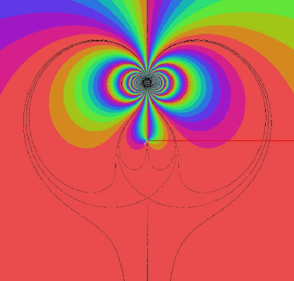
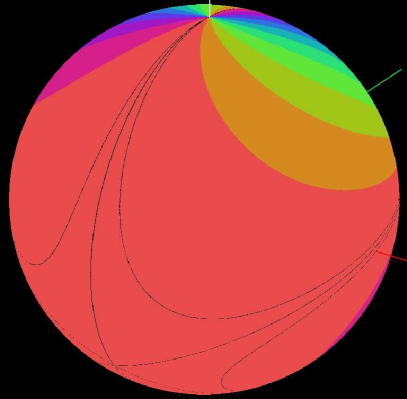
Figure 7. Visualization of the field $X(z)=\frac{z(2z-i)^{2}}{(2z+i)^{2}}\frac{\partial}{\partial z}$. (a) Shows a vicinity of the origin and one can observe a simple zero at the origin, a double zero at $\frac{i}{2}$, and a double pole at $-\frac{i}{2}$. (b) Shows the vector field on the Riemann sphere where one can see a simple zero at $\infty\in{\widehat{\mathbb{C}}}$ and an order 2 pole at $-\frac{i}{2}$.

8.1.2. The case of $X(z)=-\frac{z^{2}(z-1)}{z^{2}-z+1}\frac{\partial}{\partial z}$

This corresponds to Example 12.2, that is the rational vector field

$X(z)=-\frac{z^{2}(z-1)}{z^{2}-z+1}\frac{\partial}{\partial z}$.

In Figure 8 we present the visualization of the phase portrait. As can be observed the borders of the strip flows correspond to streamlines of the field. We are also plotting some explicit trajectories that pass through the poles (of order $-1$ at the roots of $z^{2}-z+1$) and zeros (of order 2 at 0 and of order 1 at 1 and $\infty$) of the vector field.

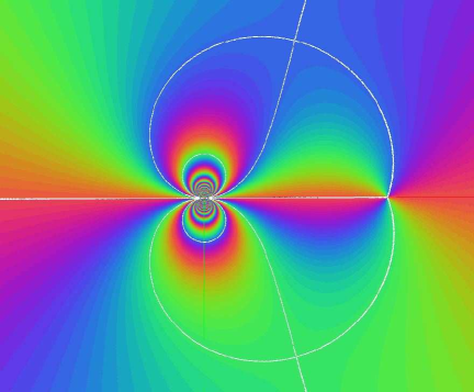
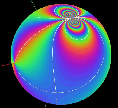
Figure 8. Visualization of the field $X(z)=-\frac{z^{2}(z-1)}{z^{2}-z+1}\frac{\partial}{\partial z}$. The borders of the strip flows correspond to streamlines of the field. We have also plotted the separatrices associated to the poles of the field.

8.2. Singular complex analytic vector fields with an isolated essential singularity at $\infty\in{\widehat{\mathbb{C}}}$

As examples of analytic vector fields with an isolated essential singularity at $\infty\in{\widehat{\mathbb{C}}}$ we present the cases of $X(z)={\text{\myfont e}}^{z}\frac{\partial}{\partial z}$ in Figure 9, and of $X(z)=\frac{{\text{\myfont e}}^{z^{3}}}{3z^{3}-1}\frac{\partial}{\partial z}$ in Figure 10. They correspond to Examples 10 and 11 so the covering maps are $\Phi_{X}(z)={\text{\myfont e}}^{{\text{\myfont e}}^{-z}}$ and $\Phi_{X}(z)={\text{\myfont e}}^{-z{\text{\myfont e}}^{-z^{3}}}$ respectively.

Worth noticing is that visualization of the phase portrait of a vector field near an essential singularity is rather difficult with the usual methods. This is due mainly to the fact that the algorithms, involving numerical integration, propagate errors along the trajectories, and Picard’s theorem tells us that near an essential singularity the vector field takes on all but at most two values in ${\widehat{\mathbb{C}}}$; hence numerical integration breaks down rather quickly near the essential singularity. Even though numerical errors are also present in our visualization scheme (as can be seen in particular in the case of Figure 10), these do not propagate along the trajectories, and are due solely to the numerical accuracy of the routines used to evaluate the auxiliary function $\rho(z)$. A deeper exploration of these errors is presented in §9.

8.2.1. The case of $X(z)={\text{\myfont e}}^{z}\frac{\partial}{\partial z}$

In Figure 9 (a), we show the strip flows on the Riemann sphere of the vector field $X(z)={\text{\myfont e}}^{z}\frac{\partial}{\partial z}$ in a vicinity of the essential singularity at $\infty$. Notice that the strips cluster together and it is difficult to appreciate the behavior of the vector field. On the other hand, by plotting specific trajectories we can examine the behavior of the flow near the essential singularity, and since the error does not propagate along the trajectory, we can visualize the actual trajectories (see Figure 9 (b)).

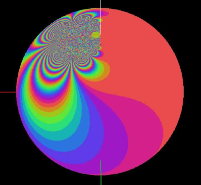
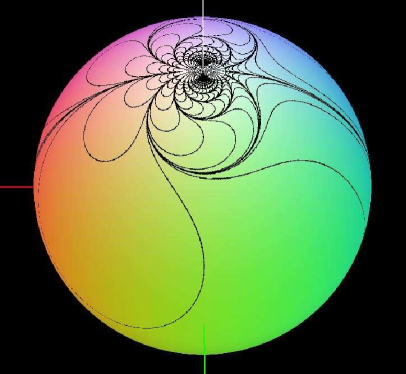
Figure 9. Visualization of $X(z)={\text{\myfont e}}^{z}\frac{\partial}{\partial z}$ near the essential singularity at $\infty$ on the Riemann sphere. In (a) we have plotted the strip flows. In (b) we have plotted some of the trajectories.

Once again, one can use the strip flows to gather information regarding the parametrization of the flow. For instance, one can observe that even though the trajectories appear symmetrical in Figure 9 (b), the strip flows in Figure 9 (a) indicate that the trajectories approach $\infty$ from the right much faster: in fact in finite time. This is a clear advantage over the results reported in [60] where only the trajectories are observed.

8.2.2. The case of $X(z)=\frac{{\text{\myfont e}}^{z^{3}}}{3z^{3}-1}\frac{\partial}{\partial z}$

In Figure 10 (a) we show the phase portrait of the vector field $X(z)=\frac{{\text{\myfont e}}^{z^{3}}}{3z^{3}-1}\frac{\partial}{\partial z}$ in the plane ${\mathbb{C}}$ where we can observe the three first order poles at $\frac{1}{\sqrt[3]{3}}$, $\frac{{\text{\myfont e}}^{i2\pi/3}}{\sqrt[3]{3}}$ and $\frac{{\text{\myfont e}}^{-i2\pi/3}}{\sqrt[3]{3}}$, while in Figure 10 (b) the phase portrait of the same vector field is shown on the sphere in a vicinity of the essential singularity at $\infty\in{\widehat{\mathbb{C}}}$.

As mentioned before, some numerical errors are still present (solid color regions near the essential singularity) due to the nature of the essential singularity of $f(z)$, but there seems to be a strong suggestion of some pattern characteristic to the essential singularities. This last remark is explored further in [5] and [7] from a theoretical viewpoint.

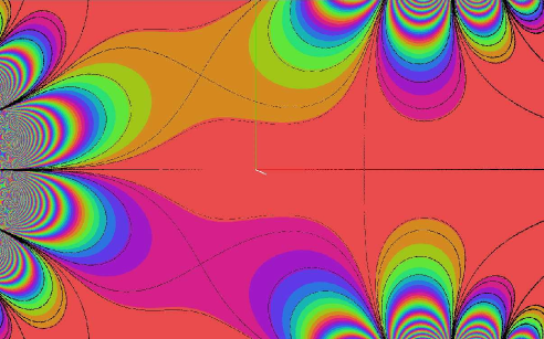
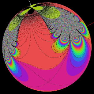
Figure 10. Visualization of $X(z)=\frac{{\text{\myfont e}}^{z^{3}}}{3z^{3}-1}\frac{\partial}{\partial z}\in{\mathscr{E}}(0,3,3)$. (a) Shows the field in the plane in a vicinity of the origin where one can observe the three simple poles at $\frac{1}{\sqrt[3]{3}}$, $\frac{{\text{\myfont e}}^{i2\pi/3}}{\sqrt[3]{3}}$ and $\frac{{\text{\myfont e}}^{-i2\pi/3}}{\sqrt[3]{3}}$. (b) Shows the field on the Riemann sphere, one can observe the essential singularity at $\infty$ and a simple pole at $\frac{{\text{\myfont e}}^{-i2\pi/3}}{\sqrt[3]{3}}$.

In particular, note that $X\in{\mathscr{E}}(0,3,3)$, hence $\Psi_{X}$ is single valued, ${\mathcal{R}}_{X}$ is an infinitely ramified Riemann surface over ${\widehat{\mathbb{C}}}_{t}$ and $\pi_{X,1}$ provides a global flow of $X$. For further details see [7], where the combinatorial concept of $(r,d)$–configuration trees allows for an accurate description of the Riemann surfaces ${\mathcal{R}}_{X}$. A very rough drawing of a generic ${\mathcal{R}}_{X}$ is provided in Figure 11.

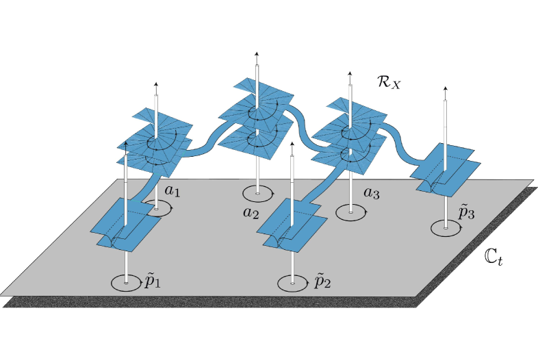
Figure 11. A sketch of a Riemann surface ${\mathcal{R}}_{X}$ for $X(z)=\frac{\lambda}{(z-p_{1})(z-p_{2})(z-p_{3})}{\text{\myfont e}}^{b_{0}z^{3}+\ldots+b_{3}}\frac{\partial}{\partial z}\in{\mathscr{E}}(0,3,3)$ according to Diagram (12). The horizontal plane is ${\mathbb{C}}_{t}$, generically there are three finite asymptotic values $\{a_{1},a_{2},a_{3}\}$ and three finite critical values $\{\widetilde{p}_{1}=\Psi_{X}(p_{1}),\widetilde{p}_{2}=\Psi_{X}(p_{2}),\widetilde{p}_{3}=\Psi_{X}(p_{3})\}$.

8.3. Singular complex analytic vector fields with an accumulation point at $\infty\in{\widehat{\mathbb{C}}}$

The third case, that in which $\infty\in{\widehat{\mathbb{C}}}$ is an accumulation point of zeros or poles of $f(z)$ is also of interest. Here we present two examples:

8.3.1. The case of $X(z)=-\tan(z)\frac{\partial}{\partial z}$

As was seen in Example 8, the ramified covering characterizing this vector field is $\Phi(z)=\sin(z)$. In Figure 12 we provide the visualization of the phase portrait of $X$. Clearly we observe a sequence of alternating simple poles and zeros along the real axis accumulating to $\infty\in{\widehat{\mathbb{C}}}$.

By plotting the separatrices associated to the poles we can immediately observe their position. It should be noted that in this case the separatrices are also horizontal asymptotic paths associated to the (non–isolated) essential singularity at $\infty\in{\widehat{\mathbb{C}}}$.

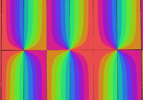
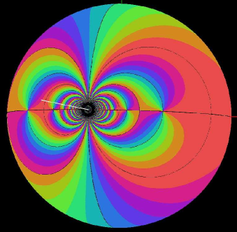
Figure 12. The field $X(z)=-\tan(z)\frac{\partial}{\partial z}$ visualized in the complex plane and on the Riemann Sphere, using the techniques described in the text. One can observe a sequence of alternating simple poles and zeros along the real axis accumulating to $\infty\in{\widehat{\mathbb{C}}}$.

8.3.2. The case of $X(z)=-(\cosh(z)+1)\frac{\partial}{\partial z}$

The ramified covering that characterizes this vector field is given by $\Phi(z)={\text{\myfont e}}^{\frac{{\text{\myfont e}}^{z}-1}{{\text{\myfont e}}^{z}+1}}$, as was remarked previously in Example 9. The visualization of the phase portrait of $X$ is provided in Figure 13. We observe a sequence of order two zeros along the imaginary axis accumulating to $\infty\in{\widehat{\mathbb{C}}}$.

Notice that $X$ does not have any poles, hence there are no separatrices. However by plotting some specific level curves we can observe some of the horizontal asymptotic paths associated to the the (non–isolated) essential singularity at $\infty\in{\widehat{\mathbb{C}}}$. Thus the behaviour of the flow of $X$ on neighborhoods of $\infty\in{\widehat{\mathbb{C}}}$ is better understood.

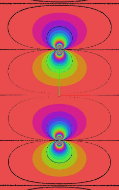
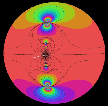
Figure 13. The field $X(z)=-(\cosh(z)+1)\frac{\partial}{\partial z}$ visualized in the complex plane and on the Riemann Sphere, using the techniques described in the text. In this case one observes a sequence of zeros of order 2 along the imaginary axis accumulating to $\infty\in{\widehat{\mathbb{C}}}$.

9. Comparison with usual integration–based algorithms

In this section we compare the proposed method with two of the most widely used integration–based algorithms: namely with the $4^{th}$ order Runge–Kutta (RK4) and the Runge–Kutta–Fehlberg (RKF) algorithms. We do not consider Euler’s method because it uses a first order approach and its results are expected to be worse than those obtained by the Runge–Kutta algorithms.

As seen in §4.2, given a singular complex analytic vector field $X(z)=f(z)\frac{\partial}{\partial z}$ the generic behaviour of the flow is different in the neighborhood of:

1. non–singular points of $X(z)$,

2. singular points of $X(z)$, which are further subdivided as

   1. zeros,

   2. poles,

   3. essential singularities and

   4. accumulation points of the above types.

We compare the behaviour in cases (1), (2a), (2b) and (2c) above using

1. two integration–based algorithms:

   1. $4^{th}$ order Runge–Kutta algorithm (RK4),

   2. Runge–Kutta–Fehlberg algorithm (RKF), and

2. the Newton method proposed in this note.

The integration–based algorithms, RK4 and RKF, are usually used to solve first order ODE systems. The RK4 is a constant step-size method whose implementation is very simple and well known, however one does not have control over the error incurred. The Runge–Kutta–Fehlberg is an adjustable step-size method which allows some control on the error. This method is a combination of the Runge–Kutta of order four and five, hence is also known as RKF45. For further information and explicit implementations of these algorithms consult [12].

Since the Newton method proposed in this note provides us with exact solutions to the problem of finding trajectories (including parametrization) of the flow of a given complex analytic vector field, then it is possible to calculate the (absolute) error involved while using integration–based algorithms:

Let $\tilde{z}_{\tau}=\tilde{z}(\tau)$ denote the trajectory that passes through $z_{0}$ at time $\tau=0$ obtained using an integration–based algorithm, and let $z_{\tau}=z(\tau)$ denote the exact solution obtained with the Newton method. Then the absolute error incurred by the integration–based algorithm is given by

(32) $$\text{AbsErr}(\tau)=\left\lvert z_{\tau}-\tilde{z}_{\tau}\right\rvert.$$

So, in order to calculate the error at time $t$ one has to:

1. calculate $\tilde{z}_{\tau}$ using the integration–based algorithm,

2. calculate $z_{\tau}$ as the intersection of $\rho(z)=\rho(z_{0})$ with $\theta(z)=\theta(z_{0})-\tau$,

3. calculate the error using (32).

On the other hand, the error of the exact solution (i.e. the one obtained with the Newton method) can be estimated by an indirect method as the relative deviation of the exact solution given by

$$\text{RelDev}_{h}(\tau)=\frac{\left\lvert\rho(z_{\tau})-\rho(z_{0})\right\rvert}{\left\lvert\rho(z_{0})\right\rvert}.$$

This measurement can be interpreted as the unit–less distance of the calculated point $z_{\tau}$ from the actual trajectory. Moreover using this indirect method, one can also measure the deviation that the integration–based algorithms have from the exact solution by calculating the relative error of the integration–based solution as:

$$\text{RelError}_{h}(\tau)=\frac{\left\lvert\rho(\tilde{z}_{\tau})-\rho(z_{0})\right\rvert}{\left\lvert\rho(z_{0})\right\rvert}.$$

These last two measurements can be used to compare side by side the solution obtained by the Newton method and the integration–based methods.

9.1. Results of the comparison

We compared the associated errors obtained by the usual integration methods vs. the exact solution obtained with the proposed methodology; also the CPU time used by the different approaches is reported.

In all cases we restricted our analysis to a rectangular region of the plane, since to visualize the results on the Riemann sphere stereographic projection is used independently of which visualization method is chosen, hence this restriction does not affect the comparison results.

This was done in neighborhoods of: a regular (R) value of the flow, a zero (Z) of $f$, a pole (P) of $f$, and an essential singularity (E) of $f$. The different errors $\big{(}\text{AbsErr}(t)$, $\text{RelDev}_{h}(t)$ and $\text{RelError}_{h}(t)\big{)}$ were plotted as a function of $\tau$ in a vicinity of $\tau=0$ resulting in Figures 14 (a), 15 (a), 16 (a), 17 (a) for the case of the $4^{th}$ order Runge–Kutta algorithm; and in Figures 14 (b), 15 (b), 16 (b), 17 (b) for the case of the Runge–Kutta–Fehlberg algorithm.

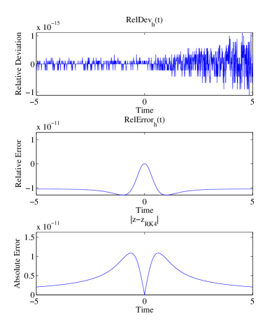
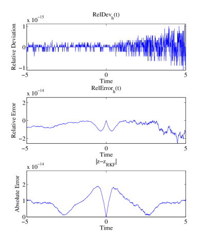
(a)                                                          (b)

Figure 14. Comparison of the errors in a vicinity of a regular point obtained (a) when using the $4^{th}$ order Runge–Kutta algorithm, and (b) when using the Runge–Kutta–Fehlberg algorithm. The vector field $\exp(z)\frac{\partial}{\partial z}$ was used with initial condition $z_{0}=i\frac{\pi}{2}$.

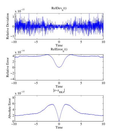
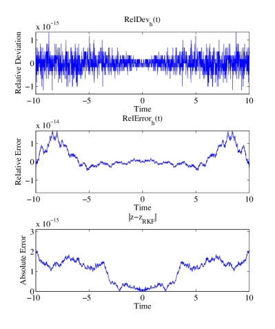
(a)                                                          (b)

Figure 15. Comparison of the errors in a vicinity of a zero obtained (a) when using the $4^{th}$ order Runge–Kutta algorithm, and (b) when using the Runge–Kutta–Fehlberg algorithm. The vector field $z^{4}\frac{\partial}{\partial z}$ was used with initial condition $z_{0}=\frac{i}{2}$.

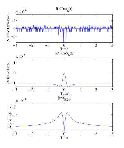
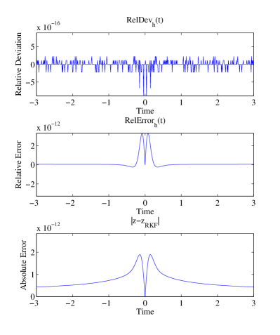
(a)                                                          (b)

Figure 16. Comparison of the errors in a vicinity of a Pole obtained (a) when using the $4^{th}$ order Runge–Kutta algorithm, and (b) when using the Runge–Kutta–Fehlberg algorithm. The vector field $\frac{1}{z}\frac{\partial}{\partial z}$ was used with initial condition $z_{0}=-\frac{1}{2}-i\frac{1}{2}$.

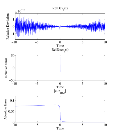
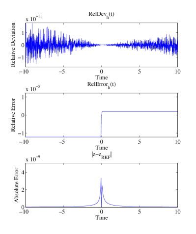
(a)                                                          (b)

Figure 17. Comparison of the errors in a vicinity of an isolated essential singularity obtained (a) when using the $4^{th}$ order Runge–Kutta algorithm, and (b) when using the Runge–Kutta–Fehlberg algorithm. The vector field $-z^{2}\exp(\frac{1}{z})\frac{\partial}{\partial z}$ was used with initial condition $z_{0}=0.1-i0.066$.

As for a measure of the computational resources, we report the CPU time used by the algorithms in calculating the trajectories. In order to have a more realistic scenario, we measured the time it took to calculate the trajectories starting at 5 different initial conditions $z_{0}$ in each vicinity and report the average times obtained. We report these times for each of the different generic neighborhoods in Table 2.

Table 2. Average CPU time (measured in seconds) used for the calculation of 5 selected trajectories with the distinct algorithms, and for the calculation of the complete (global) field. The integration-time interval chosen was 500 time units.

	Time in seconds	Time in seconds	Time in seconds	Time in seconds
Type of	using Newton	using $4^{th}$ order	using RKF	for the calculation
neighborhood	method	RK4 algorithm	algorithm	of the global field
regular point (R)	0.026	0.042	0.252	0.844
singular point (Z)	0.591	0.892	0.312	0.884
singular point (P)	0.492	0.627	0.312	0.887
singular point (E)	0.420	0.652	0.358	0.830

9.2. Discussion of the results of the comparison

9.2.1. Error comparison

As a result of examining Figures 14 thru 17, one first notices that the Newton method proposed in this note has a very small error as can be observed on the graphs of the relative deviation from the exact solution which in all cases but one remains below $10^{-15}$. Even in the case of the vicinity of an essential singularity (E) the relative deviation remains below $10^{-11}$ which is at least 6 orders of magnitude better than the same case with the use of integration–based techniques. The reason for this difference can be attributed to the fact that in a vicinity of an essential singularity the vector field has a mixture of behaviours as is further explained in (4) below.

As for the errors incurred by the integration–based algorithms, there is a marked difference in the different generic cases:

1. In the neighborhood (R) of a regular point of the flow, the errors are very small: the relative deviation (that is the relative difference in the calculated value of the constant of motion $\rho(z)$ versus the value $\rho(z_{0})$) is less than $10^{-15}$, while the relative error and the absolute error in the RK4 case is of the order of $10^{-11}$, and $10^{-14}$ in the RKF case. Hence, even when there is a difference of 3 orders of magnitude between the RK4 and the RKF case, there is only one order of magnitude difference between using the RKF algorithm and the Newton algorithm, in fact in this case the errors observed are mainly due to the numerical precision employed in the calculations.

2. In the neighborhood (Z) of a zero of $X(z)$, the errors are in fact smaller than those encountered in a vicinity of a regular point: the absolute error is of the order of $10^{-15}$ in both the RK4 and the RKF case, while the relative error and deviation differ only by one order of magnitude (even though there is a factor of 2 between the relative error of the RK4 and the RKF case). This small difference is due to the fact that the trajectories are approaching a zero, hence the trajectories tend to converge.
   In fact, in this case, the integration–based algorithms need longer integration times (hence larger computational requirements) in order to visualize the trajectories as they approach the zero. The higher the order of the zero, the longer the integration times needed to obtain the same “quality” in the visualization.

3. In the neighborhood (P) of a pole of $X(z)$, the errors behave pretty much as in the case of a regular point, except in the vicinity of $\tau=0$, where they increase quite noticeably. This is due to the fact that since the initial point $z_{0}$ of the trajectory is the closest point (on the trajectory) to the pole, this is where the values of the vector field are largest, and hence near this point is where the integration–based algorithms may fail.

4. In the neighborhood (E) of an essential singularity of $X(z)$, the errors respond in a more complicated manner, since we have a mixture of behaviours. This is expected on the following grounds: from an analytical viewpoint, one has by Picard’s Theorem that the vector field takes on all but possibly one value in ${\mathbb{C}}$ infinitively often in any neighborhood of the essential singularity, hence one expects to observe regions of behaviour similar to a pole, regions with the behaviour of a zero, and regions with behaviour similar to a regular value, all intermingled in a continuous (in fact analytical) way.
   In this case the observed errors are quite big in the case of the RK4 algorithm, mainly because almost immediately the calculated trajectory “jumps” to another trajectory that is far from the original one. This can be seen in the relative error, where one observes that the relative error is constant for most of the backward and forward trajectory but the calculated value of $\rho(z)$ is very different from the original one $\rho(z_{0})$. This same phenomena occurs in the case of the RKF algorithm, but on a much smaller scale. On the other hand, as was already observed, the relative deviation from the exact solution remains below $10^{-11}$, that is the Newton technique is quite accurate.

9.2.2. CPU time

Due to the very different nature of the integration–based algorithms and the Newton method proposed, it is rather cumbersome to actually compare the computational resources that each algorithm utilizes to visualize a given trajectory. This phenomena is due to the fact that the CPU time used when visualizing with the integration–based algorithms is directly dependent on the integration time, which in turn depends on the parametrization (speed) of the trajectory. For instance, for a trajectory that approaches a zero (Z) of the vector field, the usual methods need a very long time interval in order to visualize the phase portrait (because as time advances, the trajectories are slower), in the case of a trajectory that approaches a pole (P), the opposite is the case.

On the other hand the Newton method does not have this limitation: one of the advantages of the Newton method, lies in the fact that one visualizes the complete trajectories corresponding to the value $\rho(z_{0})$ that lie in the chosen region. When visualizing using the Newton method the time interval does not matter.

In any case, as can be observed on Table 2, the CPU time employed to calculate the trajectories behaves differently in the different generic cases: Apparently the usual integration–based techniques are faster when there are no critical values of the flow, yet as soon as one approaches a critical value of the flow the Newton method is faster than the integration–based methods. Moreover we can see an increase in CPU time in the case of the RKF method when compared with the RK4 method. It should be noticed that even though the CPU time required for the Newton method is basically the same in all scenarios, this is not the case for the RK4 and or the RKF algorithms.

It should be noticed that the CPU time taken to calculate and visualize the complete field is just 3 to 4 times longer than the CPU time required for visualizing a single trajectory.

Also we would like to point out that another disadvantage that the usual integration–based methods have and that the proposed method does not, is that in a small enough vicinity of an essential singularity the usual methods stop working, but our proposed method provides a clear visualization of the phase portrait (see Figure 18). This is mainly because convergence fails, even with the RKF algorithm, near an essential singularity.

(a)
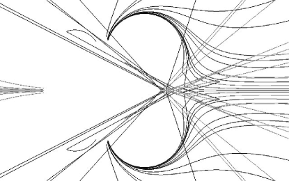
(b)
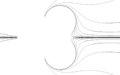
(c)

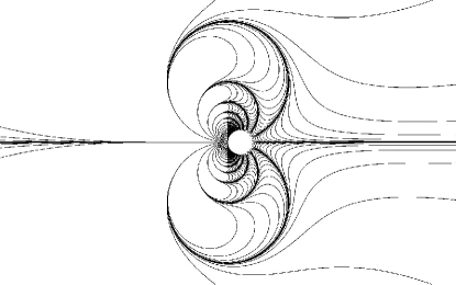
Figure 18. In this figure we have plotted the trajectories corresponding to 18 initial conditions for the vector field $\-z^{2}\exp(\frac{1}{z})\frac{\partial}{\partial z}$ in a vicinity of the essential singularity at 0. In (a) the trajectories were obtained using the RK4 algorithm, in (b) using the RKF algorithm, and in (c) with our proposed algorithm. In (a) and (b) the trajectories where plotted for forward and backward time. The initial conditions can be identified in (b) as the place where the trajectories change from gray to dark grey.

9.3. Implementation

All of the algorithms described (including the visualizations in Figures 8 thru 13 and Figure 18) were implemented using C++ and OPENGL on Mac OS X 10.5 running on a 2.16 Ghz Intel Core 2 Duo processor with 2 GB of DDR2 SDRAM.

Remark 11.

The algorithms were implemented in C++ on the Mac OS X 10.5 in order to do an accurate comparison between the usual integration methods. However, we have developed a version of the software readily available in JAVA with a function parser that can accept either

1. rational vector fields $X(z)=f(z)\frac{\partial}{\partial z}$ with $f(z)=\frac{p(z)}{q(z)}$, $p,q\in{\mathbb{C}}[z]$, or

2. a distinguished parameter $\Psi_{X}(z)=\int^{z}\frac{1}{f(\zeta)}d\zeta$, with $f(z)$ a singular complex analytic function.

This way we can visualize the singular complex analytic vector field $X(z)=f(z)\frac{\partial}{\partial z}$ both on the Riemann sphere ${\widehat{\mathbb{C}}}$ and on a user specified rectangular region of the plane ${\mathbb{C}}$. This was done so that the software could be accessible to a wider audience. The latest version can be found at

https://www.dropbox.com/sh/xfuor27nf820mwo/AAACyp0EsGx6Ain49VgUWRFMa?dl=0

10. Generalizations and open problems

In this section we present several directions that are natural to follow. We start by generalizing the techniques and method to closed Riemann surfaces. In particular, we present an example of a vector field on the torus visualized with the Newton method presented in this note.

We further present some ideas and an overview of how this can work for vector fields in ${\mathbb{R}}^{n}$, generalizing to differential manifolds of dimension $n$, and finally presenting some open (and natural) questions. Some of these problems are currently being explored by the authors and will be presented elsewhere.

10.1. Generalizing to analytic vector fields on Riemann surfaces

In order to actually implement the visualization of singular complex analytic vector fields on Riemann surfaces with the Newton method there are two obvious alternatives: using charts of the Riemann surface; and using invariant vector fields.

10.1.1. Visualization using charts

An immediate generalization of what has been presented is to visualize singular complex analytic vector fields on Riemann surfaces by using the charts associated to the Riemann surface. Note that in fact we have already done so specifically for the case of the Riemann sphere using Stereographic Projection.

The idea is simple: using charts one can do the visualization on the image in ${\mathbb{C}}$ of the chart and then return it to the Riemann surface with the inverse map of the chart (as was explained, in the case of the Riemann sphere, in §6.2).

Thus to generalize the method described above to Riemann surfaces, it is enough to take the singular complex analytic vector field $\widetilde{X}$ defined locally in $M$ and by pushforward with the coordinate of the chart $f_{\alpha}$, find the singular complex analytic vector field $X={f_{\alpha}}_{*}\widetilde{X}$ in ${\mathbb{C}}$. Since this field is a Newton vector field (by Theorem 5) then we can proceed to calculate its trajectories in ${\mathbb{C}}$ and finally take them to $M$ using $f_{\alpha}^{-1}$, thereby solving the case of Riemann surfaces.

Note that this approach also works with the usual integration–based techniques, and with other vector field visualization techniques as well. In fact in [45] they use this approach to visualize vector fields on “arbitrary surfaces”, using a texture-based approach. One of the problems that they encounter, and deal with effectively, is that visual artifacts appear when passing from one parametrization to another (that is when visualizing the vector field in $U_{\alpha}\cap U_{\beta}$ via $f_{\alpha}^{-1}$ or when visualizing the vector field using $f_{\beta}^{-1}$). This problem is expected to be present if using direct–flow visualization and geometric flow visualization techniques as well.

10.1.2. Visualization using invariant vector fields

In this case the idea is to use the fact that closed Riemann surfaces $M$ can be modeled as the quotient of the universal cover $\widetilde{M}$ of $M$ with a subgroup $\Gamma$ of the automorphism group, $\text{Aut}(\widetilde{M})$, of $\widetilde{M}$, i.e.

$$M=\widetilde{M}/\Gamma.$$

Then a complex vector field on $\widetilde{M}$ of the form

(33) $$\widetilde{X}(z)=\widetilde{f}(z)\frac{\partial}{\partial z},$$

with $\widetilde{f}(z)$ invariant under the group $\Gamma^{*}$, where $\Gamma^{*}$ denotes the group action of $\Gamma$ on the tangent vector bundle as in Lemma 2, descends to a complex vector field $X([z])$ on $M$. Thus visualizing $\widetilde{X}(z)$ on $\widetilde{M}$ is equivalent to visualizing $X([z])$ on $M$.

By the uniformization theorem of closed Riemann surfaces, $\widetilde{M}$ is either the Riemann sphere ${\widehat{\mathbb{C}}}$, the complex plane ${\mathbb{C}}$, or the hyperbolic plane ${\mathbb{H}}=\{z\in{\mathbb{C}}:{\mathfrak{Im}\left(z\right)}>0\}$. Furthermore, the first two cases produce only one more family of orientable Riemann surfaces: tori or Riemann surfaces of genus $g=1$ (which arise from considering the group $\Gamma$ generated by two non–collinear translations on ${\mathbb{C}}$). The third case produces a plethora of orientable Riemann surfaces, all of whom have negative curvature (Riemann surfaces of genus $g>1$).

In the case of tori, the class of functions which are invariant under the action of the automorphism group of a torus are called elliptic functions and have been extensively studied. In particular recall (see §7) that the first author has previously shown that all elliptic vector fields are in fact Newton vector fields [4], by showing that an elliptic function $f(z)$ can be expressed as a quotient $-\frac{\Phi(z)}{\Phi^{\prime}(z)}$, for an explicitly constructed $\Phi$ in terms of Weierstrass $\sigma$ and $\zeta$ functions (and their derivatives). Thus one can apply the techniques introduced in this paper and reduce the problem of visualizing the vector field to that of visualizing the level curves of $\rho(z)=\arg\left(\Phi(z)\right)$.

As an example, in Figure 19 the elliptic vector field

(34) $$\widetilde{X}(z)=-\frac{\wp(z)}{\wp^{\prime}(z)}\frac{\partial}{\partial z},$$

is visualized using the techniques described in this note: the strip flows of $\rho(z)=\arg\left(\wp(z)\right)$ are plotted in Figure 19 (a), moreover the corresponding vector field on the torus is visualized in Figure 19 (b). It should be noted that the vector field given by (34) was previously studied by G. F. Helminck et al., see [36] for further details. In particular they showed that up to conjugation the family of vector fields of the form (34) consist of three classes characterized by the form of the parallelogram spanned by the parameters $\omega_{1}$, $\omega_{2}$ defining $\wp(z)$. They visualized a couple of trajectories using a $4^{th}$ order Runge-Kutta integration algorithm for the case corresponding to $\omega_{1}=1$, $\omega_{2}=\frac{1}{4}+\frac{5}{4}i$, compare Figure 19 (a) with [36] figure 8.

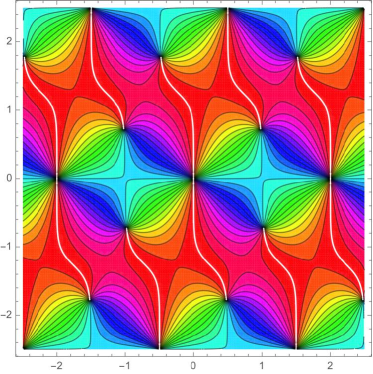
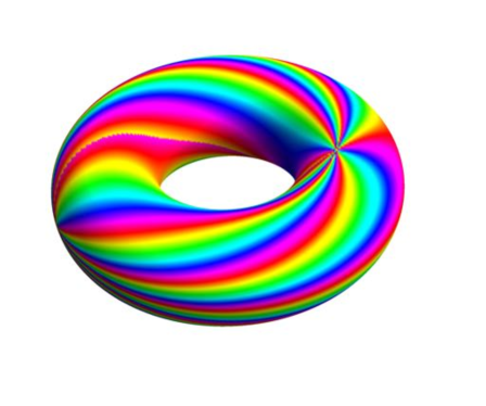
(a)                                              (b)

Figure 19. Visualization of the elliptic vector field $\widetilde{X}(z)=-\frac{\wp(z)}{\wp^{\prime}(z)}\frac{\partial}{\partial z}$. (a) on the plane and (b) the corresponding vector field on the torus. The basis $\{\omega_{1},\omega_{2}\}\subset{\mathbb{C}}$ for the underlying lattice $\Omega(\omega_{1},\omega_{2})$ is $\{\omega_{1}=1,\omega_{2}=\frac{1}{4}+\frac{5}{4}i\}$.

In the case of Riemann surfaces of genus $g>1$, a similar scheme will work: the $\Gamma$–invariant vector field $\widetilde{X}(z)$ given by (33) (which is characterized by the $\Gamma$–invariant function $\widetilde{f}(z)$ which is analytic on ${\mathbb{H}}\backslash\mathcal{S}$, where $\mathcal{S}$ is a discrete set) will be meromorphic in ${\mathbb{C}}$, and hence one will be able to explicitly represent them as Newton vector fields. Since the characterization of the $\Gamma$–invariant meromorphic functions, for the case of genus $g\geq 3$, is a whole subject on its own, the visualization of vector fields on Riemann surfaces of genus $g\geq 3$ is left for future work.

10.2. Generalizing to vector fields in ${\mathbb{R}}^{n}$

In this direction there is already some work reported in the literature: in 1988 S. A. Burns and J. I. Palmore [18] presented a generalization of some of the techniques they developed in [62], to some vector fields in ${\mathbb{R}}^{n}$. In §10.2.1 we present an overview of these techniques and mention some of its limitations.

An alternative generalization that is based upon the present work, but uses commutative algebras with unity, instead of the complex number field, is outlined in §10.2.2.

10.2.1. Vector–valued Newton method in ${\mathbb{R}}^{n}$

Since the results presented in this section have been published elsewhere (see [62], [18]), we only give a rough sketch of the steps that need to be followed, without going into the details.

Given a differentiable function $F:{\mathbb{R}}^{n}\to{\mathbb{R}}^{n}$, locally one–to–one, and with a differentiable inverse, then $F$ defines the following vector field

$$H(x)=-\left[DF(x)\right]^{-1}F(x),$$

where $DF(x)$ is the Jacobian matrix of partial derivatives. This vector field is known as the Newton vector field associated to $F$.

On the other hand, given a vector field $H(x)$, it is possible to show that in a neighborhood of a regular point $x_{0}$ of $H$ with $H(x_{0})\neq 0$, there exists $F:{\mathbb{R}}^{n}\to{\mathbb{R}}^{n}$ such that $H$ is the Newton vector field associated to $F$. Also, $H$ and $F$ satisfy

(35) $$DF(x)H(x)=-F(x).$$

This last equation, as in the complex case, is intimately linked to the solutions of

(36) $$\frac{dx}{d\tau}=H(x),$$

since if $x(\tau)$ satisfies

$$F(x(\tau))={\text{\myfont e}}^{-(\tau-\tau_{0})}F(x(\tau_{0})),$$

then $x(\tau)$ is a trajectory solution of (36). Hence, by considering $F=(F_{1},F_{2},\cdots,F_{n})$ and $H=(H_{1},H_{2},\cdots,H_{n})$ the relation (35) can be re-written as

$$H(x)\cdot\nabla F_{i}(x)=-F_{i}(x),\ i=1,2,\cdots,n.$$

so by proposing that the $F_{i}$ be of the form $F_{i}=\exp\left[G_{i}\right]$ one has

$$H(x)\cdot\nabla G_{i}(x)=-1,$$

and each difference $G_{ij}=G_{i}-G_{j}$ satisfies

$$H(x)\cdot\nabla G_{ij}(x)=0,$$

so that the $G_{ij}$ are constant on the trajectories of $\frac{dx}{d\tau}=H(x)$.

Note that in this case, as opposed to the complex case, one still has to solve a system of differential equations to find the auxiliary functions $G_{ij}$, but these equations are usually much simpler to solve than the original ones that define the trajectories and that are solutions to (36). In a couple of cases examined in [62], [18] these auxiliary functions $G_{ij}$ can be found, but there is no known technique that works in general.

10.2.2. Generalized analytic functions and the Newton method

An alternative to the previous method that will work for a large class of vector fields has been presented by some of the authors in [8]. It is based upon the notions of generalized analytic functions: the basic idea is that under certain conditions one may define a commutative algebra with unity of dimension $n$. Moreover, the differentiable functions of the algebra satisfy certain “Cauchy–Riemann equations”, in an analogous manner as the case of the usual analytic functions over ${\mathbb{C}}$ (hence these functions are also called generalized analytic functions).

Once this commutative algebra with unity is defined, one can develop an analog of analytic function theory for these generalized analytic functions, so that finally the scheme presented in this note can be carried over to the algebra, providing a framework where the generalized analytic vector fields can be visualized by the same techniques.

For instance in the case of dimension 2, the class of vector fields for which this generalization will work, includes the real valued vector fields

$$F(x,y)=u(x,y)\frac{\partial}{\partial x}+v(x,y)\frac{\partial}{\partial y},$$

whose Jacobian matrix of partial derivatives is of the form $AJA^{-1}$, where $A$ is an invertible matrix and $J$ is a matrix in one of the following normal forms

$$\begin{pmatrix}a&b\\ -b&a\end{pmatrix},\qquad\begin{pmatrix}a&b\\ 0&a\end{pmatrix},\qquad\begin{pmatrix}a&0\\ 0&b\end{pmatrix}.$$

Further work related to vector fields in this direction can be found in [24].

10.3. Generalizing to vector fields on differentiable $n$–dimensional manifolds

Once the issue of visualizing vector fields in ${\mathbb{R}}^{n}$ is solved, an immediate option is to generalize this to differentiable $n$-dimensional manifolds, once again using the charts associated to the differentiable manifolds, or by using invariant vector fields on the universal cover. The description is completely analogous to the one given in §10.1.1 and §10.1.2, so we omit it.

11. Application: Visualizing complex functions

As an application of the proposed geometrical method for visualizing singular complex analytic vector fields, we look into the problem of visualizing complex functions.

The naive approach of visualization of complex functions by their graph fails on account of a simple dimension count: the domain and range of complex functions require two real dimensions each, thus the graph is simply a (real) two dimensional surface embedded in (real) four dimensional space. This is not easy to visualize because of our natural limitation to visualize (real) three dimensional space. Thus it is not surprising that complex analysis has made huge advances with a symbolic/algebraic approach.

However, with the advent of computers and the ease of use of them as tools for visualizing mathematical objects, there has been a dramatic increase in the geometrical aspects of complex analysis. In particular, a related topic with beautiful images is the iteration of complex functions. As far as we know, it was B. Mandelbrot who first considered images of iterations, introducing what is now known as the Mandelbrot set [52]; later on the work of R. L. Devaney (see [3] §4, and [22]), P. Blanchard [11], J. Milnor [55] and many others, made iteration of complex functions known to a much wider audience. Nowadays this is an area of intense and very productive research.

For the visualization of complex functions, a starting point which includes diverse articles, course materials and applets is “Websites related to Visual Complex Analysis” [73].

In this section we do a quick review of some of the more common visualization techniques, emphasizing what exactly each technique can or can not do. One wishes to be able to distinguish zeros and poles (with their respective order/multiplicity), critical points and other singularities, in particular essential singularities.

Understanding essential singularities is much more involved than the case of zeros and poles; a reasonable first step can be found in [5], where the particular case of isolated essential singularities arising from logarithmic branch points over a finite asymptotic value $a\in{\mathbb{C}}$ is studied. In the cited work, angular sectors associated to the germ of a singular analytic vector field about an isolated essential singularity are introduced; very roughly speaking each of these new entire angular sectors consists of an infinite collection of hyperbolic and elliptic angular sectors, see Figures 7 and 8 of this work and figures 1, 2, 3 and 5 of [5].

Warning: Our discussion related to essential singularities in this section is restricted to isolated essential singularities arising from logarithmic branch points over finite asymptotic values $\{a\}\subset{\mathbb{C}}$. Many other families of essential singularities exist, for example $\infty\in{\widehat{\mathbb{C}}}$ for trigonometric functions, functions that have non conformal punctures etc., see [32] and [34].

11.1. Image of regions under $f(z)$

A classical approach investigates images of specific curves (and regions) under the mapping $f(z)$. Even though this is part of any introductory course in complex analysis and is essential for gaining an intuitive grasp of elementary functions, it is hard to implement with more general complex functions. For some readily available free software see [2], [54] and for some commercial software see for instance [46].

As an example of this technique, in Figure 20 we visualize the rational functions $f_{1}(z)=\frac{z^{3}-1}{z^{2}}$ and $f_{2}(z)=\frac{z^{2}}{z^{3}-1}$ using the image of a square region of ${\mathbb{C}}$.

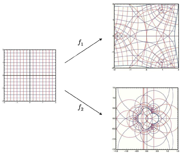
Figure 20. Example of the rational functions $f_{1}(z)=\frac{z^{3}-1}{z^{2}}$ and $f_{2}(z)=\frac{z^{2}}{z^{3}-1}$ visualized using the image of the square region $[-2,2]\times[-2,2]\subset{\mathbb{C}}$.

As it is clear from this example, by pushing forward the image, the result is a multivalued map which makes it difficult to “read–off” the information regarding the map. This technique works best with small domains.

Advantages: easy to understand and present, even in elementary courses.

Disadvantages: hard to implement for general complex functions, moreover it is not easy to “read” the information regarding the function.

11.2. Tilings a la Klein

To avoid the previously encountered difficulty, it is possible to use the pullback. In this direction, a technique pioneered, as far as we know, by F. Klein in his “Protokolle”, see [41] and [20], is the following.

Let $f:{\widehat{\mathbb{C}}}_{z}\longrightarrow{\widehat{\mathbb{C}}}_{w}$ be a complex analytic function, and let

$R_{f}=\{w_{0},w_{1},\ldots,w_{s}\}\subset{\widehat{\mathbb{C}}}_{w}$

be its set of ramification values, and

$C_{f}=\{c_{0},c_{1},\ldots,c_{\ell}\}\subset{\widehat{\mathbb{C}}}_{z}$

its critical set. The simplest case is when $f$ is a rational function (moreover, the method applies for more general classes of functions).

Secondly, let $\gamma\subset{\widehat{\mathbb{C}}}_{w}$ be an oriented Jordan path running through $R_{f}$. Then ${\widehat{\mathbb{C}}}_{w}\backslash\gamma$ is the union of two open simply connected domains.

Recognizing ${\widehat{\mathbb{C}}}_{w}\backslash\gamma$ as a two color tiling of the sphere, the pullback $f^{*}\gamma$ determines a second tiling ${\widehat{\mathbb{C}}}_{z}\backslash f^{*}\gamma$. That is

$$(f,\gamma)\longrightarrow f^{*}\gamma.$$

For example if $f$ is a rational function of degree $d$, the number of tiles in ${\widehat{\mathbb{C}}}_{z}\backslash f^{*}\gamma$ is $2d$. In Figure 21 we visualize as an example the rational functions $f_{1}(z)=\frac{z^{3}-1}{z^{2}}$ and $f_{2}(z)=\frac{z^{2}}{z^{3}-1}$.

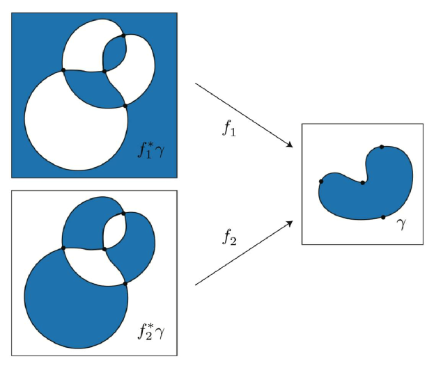
Figure 21. Example of the rational functions $f_{1}(z)=\frac{z^{3}-1}{z^{2}}$ and $f_{2}(z)=\frac{z^{2}}{z^{3}-1}$ visualized with tilings a la Klein. In both cases there are four critical points and four critical values.

It is to be noted that unless the poles and zeros of the function $f$ are critical points, the poles and zeros will be undistinguishable by this technique.

Table 3. Interpretation of tilings of $f^{*}\gamma$

Function $f$	Tiling of $f^{*}\gamma$
$z_{0}$ is a simple
zero of $f$
$z_{0}$ is a simple
pole of $f$
$z_{0}$ is an isolated essential	$z_{0}$ is a vertex of the tiling
singularity of $f$	with infinite tiles bordering it
$z_{0}$ is a critical point	$z_{0}$ is a vertex of the tiling
of order $k$	with $2k$ tiles bordering it

Advantages: the procedure can be done by hand: for rational functions it is simple. However, it also works for infinite ramified coverings $f:M\longrightarrow{\widehat{\mathbb{C}}}$.

Disadvantages: considers the critical points (that can be regular points) of $f$, not the zeros or poles. Depends strongly on the choice of $\gamma$, in fact the method “visualizes” pairs $(f,\gamma)$: changing $\gamma$ for fixed $f$ determines very different tilings.

11.3. Analytical landscapes

Another traditional concept for visualizing complex functions is the so called analytical landscape, apparently introduced by E. Maillet [51] in 1903, which basically is a graph of the absolute value $\left\lvert f(z)\right\rvert$ of a complex function $f(z)$,

$$f(z)\longrightarrow\{(z,\left\lvert f(z)\right\rvert)\ |\ z\in{\mathbb{C}}\}.$$

Of course, even though useful, not all the information of the function $f(z)$ could be conveyed: the argument of $f(z)$ was lost. However by drawing also the lines of constant argument this could be solved. Even better, by use of colormaps it is possible to draw colored analytic landscapes where isochromatic lines correspond to lines of constant argument. See Figure 22.

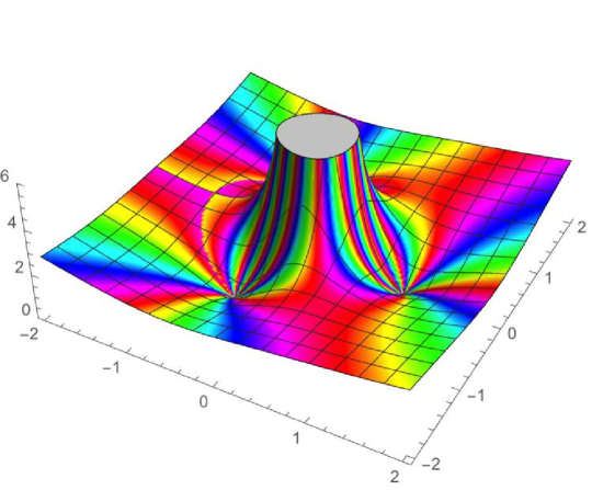
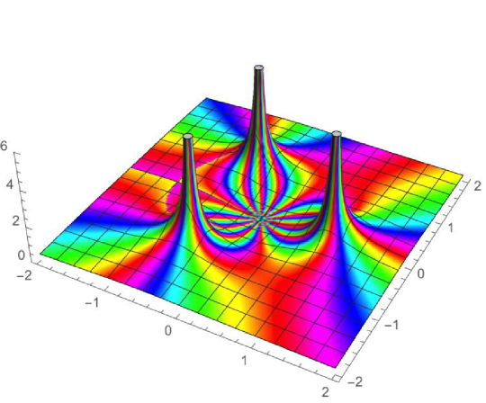
Figure 22. Example of the rational functions $f_{1}(z)=\frac{z^{3}-1}{z^{2}}$ and $f_{2}(z)=\frac{z^{2}}{z^{3}-1}$ visualized with the colored analytic landscape technique.

However, there is an inherent difficulty of reading off the information related to the function $f(z)$ when some of the essential parts might be hidden in the valleys behind the mountain rims or covered by towers of poles.

Advantages: useful, particularly the colored analytical landscapes since it contains complete information of the function $f(z)$.

Disadvantages: inherent difficulty reading off the information related to the function, since it is a three dimensional image projected onto two dimensions.

In these situations, the best one can do is to view the colored analytic landscape straight from the top. The result is a flat color image sometimes called the phase portrait of $f(z)$, representing the color coded phase or argument of $f(z)$,

$$f(z)\longrightarrow\arg\left(f(z)\right).$$

According to E. Wegert [72], the phase is better suited than the modulus to understand a function and to reconstruct the properties of $f(z)$. This alternative approach using colormaps for coloring the domain of $f(z)$ is called domain colorings.

11.3.1. Domain colorings

The main idea is to pullback the color, i.e. assign a color to each point of the range of $f(z)$ and then color each point $z$ of the domain of the function according to the color of its image $f(z)$. Apparently these were first used in the WWW by F. Farris [23].

A very common colormap is to use the polar form of complex numbers to assign a color to each point on the range ${\widehat{\mathbb{C}}}$; the magnitude is assigned an intensity or brightness (0 is assigned black, $\infty$ is assigned white, or vice versa), while the argument is mapped to a “rainbow” color wheel using the polar form of complex numbers. It is clear that phase portraits are a special form of domain colorings where the modulus of $f(z)$ is ignored.

Let us look a little more in detail on how phase portraits of functions convey the information related to the function $f(z)$. An order $s$ zero of $f(z)$ is seen as a rainbow color wheel repeated exactly $s$ times around the placement of the zero, with the color wheel following the same arrangement as in the range about the origin. On the other hand, an order $-\kappa\leq-1$ pole of $f(z)$ is seen as a rainbow color wheel repeated exactly $\kappa$ times around the placement of the pole, with the color wheel following the opposite arrangement as in the range about the origin. In other words, if we do not know the color map associated to the range it is impossible to distinguish between a pole and a zero; this same idiosyncrasy appears also when we have a gray colored image. See Figure 23 for an example of a phase portrait for the two functions $f_{1}(z)=\frac{z^{3}-1}{z^{2}}$ and $f_{2}(z)=\frac{z^{2}}{z^{3}-1}$.

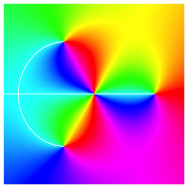
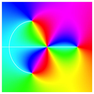
Figure 23. Example of the rational functions $f_{1}(z)=\frac{z^{3}-1}{z^{2}}$ and $f_{2}(z)=\frac{z^{2}}{z^{3}-1}$ visualized by their phase portrait. It is impossible to distinguish a pole from a zero unless we know beforehand the colormap used. Note that the order of the pole or zero is distinguished by the number of repeated color wheels around the pole or zero.

Identifying isolated essential singularities and/or accumulation points of poles, zeros or essential singularities is easy: they are characterized by the fact that any neighborhood of the singularity intersects infinitely many isochromatic lines of the same color, see [72] p. 181.

On the other hand, since critical points are precisely where conformality is lost, critical points of $f$ are located where isochromatic lines form saddle points.

In Table 4 we summarize the above information.

Table 4. Domain coloring: Interpretation of phase portrait of $f$

Function $f$	Phase portrait of $f$
$z_{0}$ is an order $s\geq 1$	rainbow color wheel
zero of $f$	repeated exactly $s$ times around $z_{0}$
$z_{0}$ is an order $-\kappa\leq-1$	opposite rainbow color wheel
pole of $f$	repeated exactly $\kappa$ times around $z_{0}$
$z_{0}$ is an isolated essential	any neighborhood of the singularity
singularity of $f$	intersects infinitely many isochromatic lines
	of the same color
$z_{0}$ is a critical point	the isochromatic lines form a saddle

Advantages: easy to implement, essential singularities are easily distinguished.

Disadvantages: impossible to distinguish between a pole and a zero if the color map associated to the range is unknown.

11.4. Visualizing complex functions via the phase portrait of vector fields

The following methods use the phase portraits of certain vector fields to visualize complex functions. In order to plot the phase portrait we use the methodology developed in the preceding sections, particularly §6. A useful interpretation is expressed by the following diagram between complex analytic sections of trivial, cotangent and tangent holomorphic line bundles over $M$

(37) $$F(z)\longrightarrow dF=F^{\prime}(z)\,dz\longrightarrow\frac{1}{F^{\prime}(z)}\frac{\partial}{\partial z}.$$

Thus the real trajectories of $\frac{1}{F^{\prime}(z)}\frac{\partial}{\partial z}$ are paths whose image under $F(z)$ are horizontal lines; in other words the horizontal trajectories of the quadratic differential $(F^{\prime}(z))^{2}\,dz^{2}$.

Note that because of (24), when using the techniques developed in this work for visualizing singular complex analytic vector fields $X(z)=f(z)\frac{\partial}{\partial z}$, we have the option of using $\Psi(z)$ or $\Phi(z)$.

11.4.1. Visualizing $f(z)$ on ${\mathbb{C}}$ via $X_{f}(z)=f(z)\frac{\partial}{\partial z}$ or $\widetilde{P_{f}}(z)=\frac{1}{f(z)}\frac{\partial}{\partial z}$

In their classic work “Complex Variables” G. Polya and G. Latta propose the use of vector fields to visualize complex functions $f(z)$ on the complex plane ${\mathbb{C}}$, see [64] p. 61. Specifically, they propose the use of what is now known as the Polya vector field

$f(z)\longrightarrow P_{f}(z)={\overline{f(z)}}\frac{\partial}{\partial z}$.

They use the Polya vector field as opposed to the more immediate vector field

$f(z)\longrightarrow X_{f}(z)=f(z)\frac{\partial}{\partial z}$,

because Polya’s vector field has the following physical interpretation: a complex function $f(z)$ is analytic in a region $D\subset{\mathbb{C}}$ if its Polya vector field is differentiable, divergence free and curl free throughout the region $D$. A further advantage is that Polya’s approach can also be used to visualize and estimate complex integrals. In this direction recently, B. Braden contributes to the Polya vector field interpretation of complex integrals, see [15].

However, it is to be noted that the Polya vector field $P_{f}(z)$ is not a holomorphic vector field on $D\subset{\mathbb{C}}$; it is anti–holomorphic. This can be circumvented by recalling first that ${\overline{f(z)}}=\frac{\left\lvert f(z)\right\rvert^{2}}{f(z)}$ and secondly that multiplying a vector field by a non–vanishing scalar factor does not alter the phase portrait, it just changes the parametrization. Hence we introduce the following.

Definition 5.

Given a complex valued function $f(z)$ on $D\subset{\mathbb{C}}$, a priori $C^{0}$, considering the operator

(38) $$f(z)\longrightarrow\widetilde{P_{f}}(z)=\frac{1}{f(z)}\frac{\partial}{\partial z},$$

the image is the normalized Polya vector field of $f$.

Note that, if $f(z)$ is a complex singular analytic function then $\widetilde{P_{f}}(z)$ is a complex singular analytic vector field with the same phase portrait (but a different parametrization) as the usual Polya vector field $P_{f}(z)$.

In 1996, T. Newton and T. Lofaro [60], use $X_{f}(z)=f(z)\frac{\partial}{\partial z}$ to visualize functions of a complex variable $f(z)$; including $f(z)={\text{\myfont e}}^{z}$ on the Riemann sphere. They use Runge–Kutta–Fehlberg RKF4(5) integration based techniques to plot the flow or phase portrait of $X_{f}(z)$. Also, T. Needham [59], champions the use of vector fields for visualizing complex functions; however he does not propose any particular implementation and/or discuss visualization techniques for vector fields.

Visualizing complex functions $f(z)$ on ${\mathbb{C}}$ by plotting the phase portrait of $X_{f}(z)$ or $\widetilde{P_{f}}(z)$ provides the following mayor advantage. Because of the normal forms for meromorphic vector fields, see Proposition 2 and Figure 2, poles and zeros of vector fields are unequivocally recognized (including their order) via the topology of the phase portrait, even without color plots. For examples see Figures 7, 8 and 24.

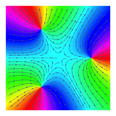
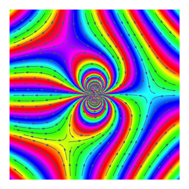
Figure 24. Example of the rational functions $f_{1}(z)=\frac{z^{3}-1}{z^{2}}$ and $f_{2}(z)=\frac{z^{2}}{z^{3}-1}$ visualized as $X_{f_{1}}(z)=f_{1}(z)\frac{\partial}{\partial z}$ and $X_{f_{2}}(z)=f_{2}(z)\frac{\partial}{\partial z}$ respectively. In this case there is no problem distinguishing between the two functions and all the information can be read from the plots. Note that the phase portrait of $X_{f_{1}}(z)$ and $P_{f_{2}}(z)$ are the same (with a different parametrization), similarly $X_{f_{2}}(z)$ and $P_{f_{1}}(z)$ have the same phase portrait.

The phase portraits of singular analytic vector fields with isolated essential singularities arising from logarithmic branch points over finite asymptotic values $\{a\}\subset{\mathbb{C}}$, can with distinguished by the presence of entire angular sectors, see [5] §5.2 for the appropriate definitions. Examples can be found in Figures 9, 10 and more examples in [5] and [6].

However, a mayor flaw related to visualizing a function $f(z)$ on an arbitrary Riemann surface $M$ via the normalized Polya vector field $\widetilde{P_{f}}(z)={\overline{f(z)}}\frac{\partial}{\partial z}$, or the vector field $X_{f}(z)=f(z)\frac{\partial}{\partial z}$, is that considered as tensors $f(z)$ and $\widetilde{P_{f}}(z)$ (or $X_{f}(z)$) are quite different: i.e. when acted upon by $Aut(M)$ they do not transform in the same way. This is made evidently clear in the following example.

Example 15.

Consider $f(z)=\frac{z^{2}}{(z-1)^{2}}$ on the Riemann sphere ${\widehat{\mathbb{C}}}$. Of course $\infty\in{\widehat{\mathbb{C}}}$ is a regular point. However when considering

$X_{f}(z)=\frac{z^{2}}{(z-1)^{2}}\frac{\partial}{\partial z}$  or  $\widetilde{P_{f}}(z)=\frac{(z-1)^{2}}{z^{2}}\frac{\partial}{\partial z}$

on ${\widehat{\mathbb{C}}}$, each has a double zero at $\infty\in{\widehat{\mathbb{C}}}$. Considering rational functions $f$ and vector fields $X$ on any compact Riemann surface $M$ of genus $g$, topological invariants are the Chern class of the trivial and tangent holomorphic line bundles as follow

$$\#\hbox{zeros}(f)-\#\hbox{poles}(f)=0,\ \ \ \#\hbox{zeros}(X)-\#\hbox{poles}(X)=2-2g.$$

A summary of the information that can be observed with this visualization technique is presented in Table 5.

Table 5. Visualization of $f$ via phase portrait of $X_{f}(z)=f(z)\frac{\partial}{\partial z}$ and $\widetilde{P_{f}}(z)=\frac{1}{f(z)}\frac{\partial}{\partial z}$

Function $f$	Phase portrait of	Phase portrait of
	$X_{f}(z)=f(z)\frac{\partial}{\partial z}$	$\widetilde{P_{f}}(z)=\frac{1}{f(z)}\frac{\partial}{\partial z}$
$z_{0}$ is a simple zero of $f$	angular sector corresponding	4 hyperbolic angular sectors
	to a center	around $z_{0}$
$z_{0}$ is an order $s\geq 2$	$2(s-1)$ elliptic angular	$2(s+1)$ hyperbolic angular
zero of $f$	sectors around $z_{0}$	sectors around $z_{0}$
$z_{0}$ is a simple pole of $f$	4 hyperbolic angular sectors	angular sector corresponding
	around $z_{0}$	to a center
$z_{0}$ is an order $-\kappa\leq-2$	$2(\kappa+1)$ hyperbolic angular	$2(\kappa-1)$ elliptic angular
pole of $f$	sectors around $z_{0}$	sectors around $z_{0}$
$z_{0}$ is an isolated essential	infinitely many elliptic	infinitely many elliptic
singularity of $f$	and hyperbolic sectors	and hyperbolic sectors
	around $z_{0}$	around $z_{0}$
$z_{0}$ is a critical point
	trajectory of $X_{f}$	trajectory of $\widetilde{P_{f}}$

Advantages: easily distinguishes key features of the function (zeros, poles, isolated essential singularities and accumulation points of any of the above), even without color plots.

Disadvantages: it is not global in nature: because of the different tensor type between $f$ and $X_{f}$ or $\widetilde{P_{f}}$, this technique will work on charts, but not necessarily on the whole Riemann surface $M$ where $f$ is defined. Moreover, the critical points of $f(z)$ are not immediately appreciated.

11.4.2. Visualizing the functions $\Psi_{X}(z)$ on $M$ via the vector fields $X(z)=\frac{1}{\Psi_{X}^{\prime}(z)}\frac{\partial}{\partial z}$ or $\widetilde{P}_{X}(z)=\Psi^{\prime}_{X}(z)\frac{\partial}{\partial z}$ (via the singular analytic dictionary)

An alternative that avoids the above mentioned problems is to use (1) of Theorem 2.

From the correspondence given by the singular complex analytic dictionary (Proposition 1) and Diagram 3, use

$X(z)=\frac{1}{\Psi^{\prime}_{X}(z)}\frac{\partial}{\partial z}$ as a way of visualizing the complex functions $\Psi_{X}(z)$.

It should be noted that this is in fact the visualization of the complex integral of the 1–form $\omega_{X}$ associated to the vector field $X(z)$.

More precisely considering (37) with $\Psi_{X}(z)$, we observe that

(39) $$\Psi_{X}(z)\longrightarrow X(z)=\frac{1}{\Psi^{\prime}_{X}(z)}\frac{\partial}{\partial z}.$$

Of course we can also consider the normalized Polya vector field

(40) $$\Psi_{X}(z)\longrightarrow\widetilde{P_{X}}(z)=\Psi^{\prime}_{X}(z)\frac{\partial}{\partial z}.$$

Note that simple zeros of $\Psi_{X}(z)$ can not be distinguished since they correspond to regular points for the vector fields, however the critical points of $\Psi_{X}$ appear as poles of $X$ and zeros of $\widetilde{P_{X}}$, hence critical points of $\Psi_{X}$ can not be distinguished from multiple zeros of $\Psi_{X}$. See Figure 25 and Table 6.

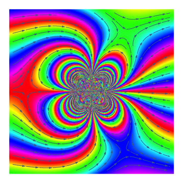
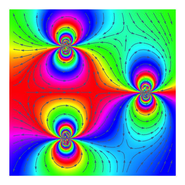
$X_{1}(z)=\frac{1}{\Psi^{\prime}_{X_{1}}(z)}\frac{\partial}{\partial z}$         $X_{2}(z)=\frac{1}{\Psi^{\prime}_{X_{2}}(z)}\frac{\partial}{\partial z}$

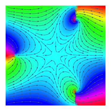
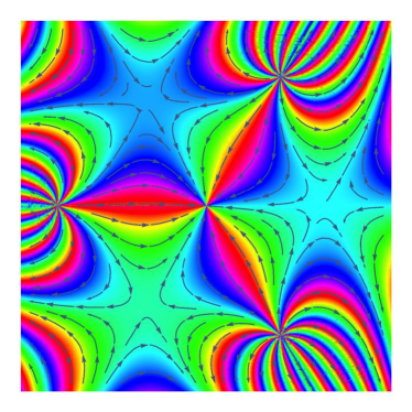
$\widetilde{P_{X_{1}}}(z)=\Psi^{\prime}_{X_{1}}(z)\frac{\partial}{\partial z}$         $\widetilde{P_{X_{2}}}(z)=\Psi^{\prime}_{X_{2}}(z)\frac{\partial}{\partial z}$

Figure 25. Visualization of the rational functions $\Psi_{X_{1}}(z)=\frac{z^{3}-1}{z^{2}}$ and $\Psi_{X_{2}}(z)=\frac{z^{2}}{z^{3}-1}$. The phase portrait of the singular complex analytic vector fields $X_{1}(z)=\frac{1}{\Psi^{\prime}_{X_{1}}(z)}\frac{\partial}{\partial z}$ and $X_{2}(z)=\frac{1}{\Psi^{\prime}_{X_{2}}(z)}\frac{\partial}{\partial z}$ is presented on the top row, and on the bottom row the phase portrait of the singular complex analytic vector fields $\widetilde{P_{X_{1}}}(z)=\Psi^{\prime}_{X_{1}}(z)\frac{\partial}{\partial z}$ and $\widetilde{P_{X_{2}}}(z)=\Psi^{\prime}_{X_{2}}(z)\frac{\partial}{\partial z}$. In this case the information of the simple zeros of $\Psi_{X_{1}}(z)$ is lost and instead information on the location of the critical points of both $\Psi_{X_{1}}(z)$ and $\Psi_{X_{2}}(z)$ appears.

Table 6. Visualization of $\Psi_{X}$ via phase portrait of $X(z)=\frac{1}{\Psi^{\prime}_{X}(z)}\frac{\partial}{\partial z}$ and $\widetilde{P_{X}}(z)=\Psi^{\prime}_{X}(z)\frac{\partial}{\partial z}$.

Function $\Psi_{X}$	Phase portrait of	Phase portrait of
	$X(z)=\frac{1}{\Psi^{\prime}_{X}(z)}\frac{\partial}{\partial z}$	$\widetilde{P_{X}}(z)=\Psi^{\prime}_{X}(z)\frac{\partial}{\partial z}$
$z_{0}$ is a simple zero of $\Psi_{X}$	$z_{0}$ is a regular point of $X$	$z_{0}$ is a regular point of $\widetilde{P_{X}}$
$z_{0}$ is an order 2 zero of $\Psi_{X}$	$z_{0}$ is a simple pole of $X$	$z_{0}$ is a simple zero of $\widetilde{P_{X}}$
	4 hyperbolic angular	angular sector
	sectors around $z_{0}$	corresponding to a center
$z_{0}$ is an order $s\geq 3$	$z_{0}$ is an order $-(s-1)\leq-2$	$z_{0}$ is an order $s-1\geq 2$
zero of $\Psi_{X}$	pole of $X$	zero of $\widetilde{P_{X}}$
	$2s$ hyperbolic angular	$2(s-2)$ elliptic angular
	sectors around $z_{0}$	sectors around $z_{0}$
$z_{0}$ is an order $-\kappa\leq-2$	$z_{0}$ is an order $\kappa+1\geq 2$	$z_{0}$ is an order $-(\kappa+1)\leq-2$
pole of $\Psi_{X}$	zero of $X$	pole of $\widetilde{P_{X}}$
	$2\kappa$ elliptic angular	$2(\kappa-2)$ hyperbolic angular
	sectors around $z_{0}$	sectors around $z_{0}$
$z_{0}$ is an isolated essential	infinitely many elliptic and	infinitely many elliptic and
singularity of $\Psi$	hyperbolic sectors	hyperbolic sectors
	around $z_{0}$	around $z_{0}$
$z_{0}$ is a critical point of $\Psi_{X}$ of	$z_{0}$ is a pole of $X$	$z_{0}$ is a zero of $\widetilde{P_{X}}$
ramification index $\mu+1\geq 2$	or order $-\mu\leq-1$	f order $\mu\geq 1$
	trajectory of $X(z)$	trajectory of $\widetilde{P_{X}}(z)$
$z_{0}$ is a logarithmic	$z_{0}$ is a simple zero	$z_{0}$ is a simple pole
singularity of $\Psi_{X}$	of $\Psi_{X}$	of $\Psi_{X}$
$\lambda\log(z-z_{0})$	$\frac{1}{\lambda}(z-z_{0})\frac{\partial}{\partial z}$	$\lambda\frac{1}{z-z_{0}}\frac{\partial}{\partial z}$
	angular sector	4 hyperbolic angular
	corresponding to a center	sectors around $z_{0}$

Advantages: has the correct tensor type behaviour, hence can be used globally on Riemann surfaces $M$. Critical points of the function $\Psi$ appear as zeros of $X_{\Psi}$ and poles of $\widetilde{P_{\Psi}}$. Logarithmic singularities of $\Psi$ appear as simple poles of $X_{\Psi}$ and simple zeros of $\widetilde{P_{\Psi}}$

Disadvantages: simple zeros of $\Psi$ are invisible, furthermore there is no way to distinguish critical points of $\Psi$ from zeros of $\Psi$ (necessarily of order $\geq 2$).

12. Complex flows

Recall the following elementary fact.

Example 16 (Complete vector fields).

A singular complex analytic vector field on a Riemann surface $M$ is complete if its flow is defined for all time and for all initial condition. A pair $(M,X)$ determine a complete vector field on a Riemann surface if and only if they appear in the following list:

1. $\big{(}{\mathbb{C}},X=P(z)\frac{\partial}{\partial z}\big{)}$ with $P$ a polynomial of degree at most 1,

2. $\big{(}{\widehat{\mathbb{C}}},X=P(z)\frac{\partial}{\partial z}\big{)}$ with $P$ a polynomial of degree at most 2,

3. $\big{(}{\mathbb{C}}^{*},X=\lambda z\frac{\partial}{\partial z}\big{)}$, with $\lambda\in{\mathbb{C}}^{*}$,

4. $\big{(}M={\mathbb{C}}/\Gamma,X=\lambda\frac{\partial}{\partial z}\big{)}$, where $M$ is a complex torus.

For a proof see [47].

The singular complex analytic dictionary (Proposition 1) allows the description of the maximal domain for the flow even in presence of poles, as we show in the following.

Example 17 (Example 2 revisited).

Let $\big{(}{\widehat{\mathbb{C}}},X=\frac{1}{R^{\prime}(z)}\frac{\partial}{\partial z}\big{)}$ be a rational vector field, for $R(z)$ a rational function of degree at least two. Then

$\Psi_{X}(z)=R(z):{\widehat{\mathbb{C}}}_{z}\longrightarrow{\mathbb{C}}_{t}$

is single valued and in accordance with Diagram (12). In this case

${\mathcal{R}}_{X}=\Omega_{X}=\big{\{}\big{(}z,R(z)\big{)}\ |\ z\in{\widehat{\mathbb{C}}}\big{\}}.$

The assertion, the global flow $\Psi^{-1}(t):\Omega_{X}\longrightarrow{\mathbb{C}}_{z}$ of $X$ starting at an initial condition $z_{0}$, makes precise sense, since

$$\Psi^{-1}:=\pi_{X,1}:{\mathcal{R}}_{X}\longrightarrow{\mathbb{C}}_{z}.$$

More generally, considering the maximal analytic continuation of the local flows, a structure for the maximal analytic continuation can be recognized as follows.

Given $z_{0}\in M^{*}$ (not a pole, essential singularity, or an accumulation point of poles, zeros or isolated essential singularities of $X$), the local flow of $X$ at $z_{0}$ is a holomorphic map

$$\begin{array}[]{rcl}\varphi_{\tt j}(z,t):\Omega(z_{0},{\tt j})\subset M^{*}\times{\mathbb{C}}_{t}&\longrightarrow&M^{*}\\ (z,t)&\longmapsto&\left\{\begin{array}[]{ll}z_{0}&\text{if }z=z_{0}\text{ is a zero of }X,\\ &\vspace{-.3cm}\\ \Psi_{\tt j}^{-1}(t)&\text{if }z\text{ is a non singular point of }X,\end{array}\right.\end{array}$$

the second case is described as $z_{1}=\Psi_{\tt j}^{-1}(t)$, where

$$\Psi_{\tt j}:z\longmapsto\int_{z}^{z_{1}}\frac{d\zeta}{f_{\tt j}(\zeta)}=t.$$

The integral is computed in a simply connected neighborhood $V_{\tt j}\subset M^{*}$ of $z_{0}$, thus $1/f_{\tt j}(\zeta)$ is holomorphic on $V_{\tt j}$, hence the map $\{\Psi_{\tt j}:z\longmapsto t\}$ is single valued. However, the value of the integral a priori depends on the choice of $V_{\tt j}$. Hence, we must fix $V_{\tt j}$ in order to construct the local flow $\varphi_{\tt j}(z,t)$. Making all these precisions, $\Omega(z_{0},{\tt j})\subset V_{\tt j}\times{\mathbb{C}}_{t}$ is an open set.

Theorem 3 (Maximal domain for the flow).

Let $X$ be a singular complex analytic vector field on a Riemann surface $M$, and let $z_{0}\in M\backslash Sing(X)$ be an initial condition.

1. The maximal analytic continuation of the local flow

   $\varphi_{\tt j}(z_{0},t):\{z_{0}\}\times({\mathbb{C}}_{t},0)\longrightarrow M^{*}$

   is univalued on the Riemann surface ${\mathcal{R}}_{X}\subset M\times{\mathbb{C}}_{t}$, which is the graph of

   $$\Psi_{X}(z)=\int_{z_{0}}^{z}\omega_{X}:M^{*}\longrightarrow{\mathbb{C}}_{t}.$$

2. The Riemann surface ${\mathcal{R}}_{X}$ is a leaf of the foliation $\mathcal{F}$ defined by the complex analytic vector field

   $$f_{\tt j}(z)\frac{\partial}{\partial z}+\frac{\partial}{\partial t}\ \ \ \hbox{ on }M^{*}\times{\mathbb{C}}_{t}$$

   and the changes of the initial conditions $z_{0}$ determine $t$–translations of ${\mathcal{R}}_{X}$.

Proof.

From the point of view of complex differential equations, $\varphi_{\tt j}(z_{0},t)=\Psi_{\tt j}^{-1}(t):\{z_{0}\}\times(\mathbb{C}_{t},0)\longrightarrow M^{*}$ for $z_{0}\in M^{0}$, is a local complex solution. Hence the map

$$\pi_{X,1}:{\mathcal{R}}_{X}\longrightarrow M,$$

together with an initial condition, $z_{0}\in M^{0}$, provides the maximal domain for the complex trajectory solution of $X$ as an ordinary differential equation determined on $M$. The Riemann surface ${\mathcal{R}}_{X}$ is a leaf of the complex analytic vector field

$$f_{\tt j}(z)\frac{\partial}{\partial z}+\frac{\partial}{\partial t}\ \ \ \hbox{ on }M^{*}\times{\mathbb{C}}_{t}.$$

The singular complex analytic foliation in the whole two dimensional complex manifold has as leaves copies of ${\mathcal{R}}_{X}$ under translations in the ${\mathbb{C}}_{t}$ factor. The maximal domain of the maximal analytic continuations of the flow for all $z_{0}\in M^{0}$ is

(41) $$\Omega_{X}=\bigcup_{t\ \hbox{translations}}{\mathcal{R}}_{X}$$

that is the domain for the assertion (3). It follows that, the complex flow $\varphi(z,t):\Omega_{X}\subset M^{*}\times{\mathbb{C}}_{t}\to M^{*}$ is completely determined by copies of one trajectory by $\pi_{X,1}$, on each connected component of $M$. ∎

Corollary 4 (From Riemann surfaces to vector fields).

Consider ${\mathbb{C}}_{t}$ provided with the vector field $\frac{\partial}{\partial t}$. The following statements are equivalent.

1. An arbitrary Riemann surface ${\mathcal{R}}\subset M\times{\mathbb{C}}_{t}$ determines a singular complex analytic vector field $X$ on $M$, following Diagram (12).

2. ${\mathcal{R}}$ is the graph of an additively automorphic map $\Psi$ as in Diagram (12).

3. The decomposition

   $\Omega_{X}=\bigcup\limits_{t\ \hbox{translations}}{\mathcal{R}}\subset M^{*}\times{\mathbb{C}}_{t}$

   determines a holomorphic foliation $\mathcal{F}$ of $\Omega_{X}$, where the leaves of $\mathcal{F}$ do not contain plaques of the form $D(z_{0},r)\times\{t_{0}\}$, for $r>0$.

Proof.

Note that, $\Psi$ is an additively automorphic map if and only if its graph ${\mathcal{R}}$ satisfies Equation (41). Hence it satisfies Diagram 12 for an appropriate $X$.

Allowing plaques of the form $\{z_{0}\}\times D(t_{0},r)$, for $r>0$, in the leaves of $\mathcal{F}$ gives rise to $X(z_{0})=0$ on $M$. Not allowing plaques of the form $D(z_{0},r)\times\{t_{0}\}$ ensures that $X$ is not identically $\infty$. A plaque different to any of the above two cases in a leaf of $\mathcal{F}$ determines locally a non identically constant $X$ on $M$. ∎

References

- [1] Ahlfors, L. V.: Conformal Invariants Topics in Geometric Function Theory, McGraw–Hill, USA, 1973.
- [2] Akers, D.: : A Tool For Visual Complex Analysis, Brown University, http://ftp.cs.brown.edu/people/dla/ma126/intro.html
- [3] Alexander, D.; Devaney, R. L.: A century of complex dynamics. In; A century of advancing mathematics, 15–34, Math. Assoc. America, Washington, DC (2015).
- [4] Alvarez–Parrilla, A.; Gómez–Arciga, A.; Riesgo–Tirado, A.: Newton vector fields on the plane and on the torus, Complex Variables and Elliptic Equations, Vol. 54, No. 5, May 2009, 440–461.
- [5] Alvarez–Parrilla, A.; Muciño–Raymundo, J.: Dynamics of Singular Complex Analytic Vector Fields with Essential Singularities I, Conform. Geom. Dyn. 21 (2017), 126–224. http://dx.doi.org/10.1090/ecgd/306
- [6] Alvarez–Parrilla, A.; Muciño–Raymundo, J.: Dynamics of Singular Complex Analytic Vector Fields with Essential Singularities II, Preprint (2018).
- [7] Alvarez–Parrilla, A.; Muciño–Raymundo, J.: Symmetries of complex analytic vector fields with an essential singularity on the Riemann sphere, (2019), 25 pages. http://arxiv.org/abs/1904.11667
- [8] Alvarez–Parrilla, A.; Frías–Armenta, M. E.; López–González, E.; Yee–Romero, C.: On solving systems of autonomous ordinary differential equations by reduction to a variable of an algebra, Int. J. Math. Math. Sci. 2012, Art. ID 753916, 21 pp.
- [9] Benzinger, H. E.: Plane autonomous systems with rational vector fields, Trans. Amer. Math. Soc. 326 (1991), no. 2, 465–483.
- [10] Berenstein, C. A., Gray, R.: Complex Variables An Introduction, Springer–Verlag, (1991).
- [11] Blanchard, P.: Complex analytic dynamics, Bull. Amer. Math. Soc. Vol. 11, Num. 1 (1984), 85–141.
- [12] Faires, J. D.; Burden, R. L.: Numerical Methods, Brooks Cole Ed., 3rd edition, 2002.
- [13] Bourke, P.: Sphere Generation, May 1992, http://local.wasp.uwa.edu.au/~pbourke/miscellaneous/sphere_cylinder/
- [14] Braden, B.: Picturing functions of a complex variable, College Math. J., 16, 1985, 63–72.
- [15] Braden, B.: Pólya’s geometric picture of complex contour integrals, Math. Mag., 60, 1987, 5, 321–327.
- [16] Branner, B.; Dias, K.: Classification of complex polynomial vector fields in one complex variable, J. Difference Equ. Appl., vol. 16, #5-6 (2010), 463–517.
- [17] Brickman, L.; Thomas, E. S.: Conformal equivalence of analytic flows, J. Diff. Eqns., vol. 25, (1977), 310–324.
- [18] Burns, S. A.; Palmore, J. I.: The Newton transform: an operational method for constructing integrals of dynamical systems, Advances in fluid turbulence (Los Alamos, NM, 1988). Phys. D 37 (1989), no. 1-3, 83–90.
- [19] Bustundy, A.; Giraldo L.; Muciño–Raymundo, J.: Jacobian mates for non–singular polynomial maps in with one-dimensional fibers, J. Singul., 9 (2014), 27–42.
- [20] Chislenko, E.; Tschinkel, Y.: The Felix Klein Protocols, Notices of the AMS. (2007), 961–970.
- [21] Dedieu, J. P.; Shub, M.: Newton Flow and Interior Point Methods in Linear Programming, International Journal of Bifurcation and Chaos, Vol. 15, No. 3 (2005), pp. 827–839.
- [22] Devaney, R. L.: An Introduction to Chaotic Dynamical Systems, Benjamin/Cummings Publishing, Menlo Park, CA, (1986).
- [23] Farris, F.: Complex Function Visualization, Santa Clara University, http://www-acc.scu.edu/~ffarris/complex.html
- [24] Frías–Armenta, M. E.; López–González, E.: On geodesibility of algebrizable planar vector fields, Boletín Soc. Mat. Mexicana, 2017, https://doi.org/10.1007/s40590-017-0186-2
- [25] Frías–Armenta, M. E.; Muciño–Raymundo, J.: Topological and analytic classification of vector fiels with only isochronous centers, J. of Difference Equations and Applications, vol 19, no. 10, (2013), 1694–1728.
- [26] Frederick, C.; Schwartz, E. L.: Conformal Image Warping, Vision Courant Institute of Mathematical Sciences and NYU Medical Center, IEEE Computer Graphics and Applications, Volume: 10, Issue: 2, March 1990.
- [27] Garijo, A., Gasull, A., Jarque, X.: Normal forms for singularities of one dimensional holomorphic vector fields, Electronic Jorunal of Differential Equations, 122 (2004), 1–7.
- [28] Garijo, A., Gasull, A., Jarque, X.: Local and global phase portait of equation , Discrete and Continuous Dynamical Systems, vol. 17, 2 (2007). 309–329.
- [29] Gluchoff, A. D.: Complex Power Series–a Vector Field Visualization, Mathematics Magazine, Vol. 66, No. 3, Jun. (1993), 189–191.
- [30] J. Gregor, Dynamické systémy s regulární pravou stranou I, Pokroky Mat. Fyz. Astron. 3 (1958), 153–160.
- [31] J. Gregor, Dynamické systémy s regulární pravou stranou II, Pokroky Mat. Fyz. Astron. 3 (1958), 266–270.
- [32] Guillot, A.: Meromorphic vector fields with single–valued solutions on complex surfaces, arXiv:1603.02288v1 [math.CV] 7 Mar 2016.
- [33] Guillot, A.: Infinitesimal actions of around isolated fixed points in the plane, Qual. Theory Dyn. Sys. 15 (2016), 433–451.
- [34] Guillot, A.: Complex differential equations and geometric structures on curves, Geometrical themes inspired by the –body problem, Springer Lecture Notes in Math., 2204 (2018) 1–47.
- [35] Hirsch, M. W.; Smale, S.: On algorithms for solving , Comm. Pure Appl. Math., 32, (1979), 281–312.
- [36] Helminck, G. F.; Kamphof, F. H.; Streng, M. and Twilt, F.: The qualitative behaviour of Newton flows for Weierstrass’ –functions, Complex Variables and Elliptic Equations, 47:10, (2002), 867–880.
- [37] Hockett, K., Ramamurti, S.: Dynamics near the essential singularity of a class of entire vector fields, Transactions of the American Mathematical Society vol. 345, N. 2 October (1994) 693–703.
- [38] Ilyashenko, Y., Yakovenko, S.: Lectures on Analytic Differential Equations, AMS, GMS 86, Providence R. I. (2008).
- [39] Kawski, M.: Interactive visualization in complex analysis, Proc. 2nd Internat. Conf. Math Teaching, Crete, Greece (2002), http://www.math.uoc.gr/~ictm2/.
- [40] Klein, F.: On Riemann’s Theory of Algebraic Functions and Their Integrals, Dover, USA, 2003.
- [41] Klein, F.: Klein Protokolle, Clay Mathematics Institute, http://www.claymath.org/publications/klein-protokolle
- [42] J. Jenkins, Univalent Functions and Conformal Mapping, Ergebnisse Der Mathematik Und Iher Grenzgebiete, Springer–Verlag, Berlin, 1958.
- [43] Langer, J.: Plotting the polyhedral geometry of a quadratic differential, Journal of Geometry, Vol. 108, No. 3 (2017), 837–849 https://doi.org/10.1007/s00022-017-0378-y
- [44] Laramee, R.; Hauser, H.; Doleisch, H.; Vrolijk, B.; Post, F. H.; Weiskopf, D: The State of the Art in Flow Visualization: Dense and Texture-Based Techniques, COMPUTER GRAPHICS forum, Vol. 23, No. 2 (2004), 203–221.
- [45] Li, G.; Tricoche, X.; Weiskopf, D.; Hansen, C.: Flow Charts: Visualization of Vector Fields on Arbitrary Surfaces, IEEE Transactions on Visualization and Computer Graphics, Vol. 14, No. 5, September/October (2008), 1067–1080.
- [46] – The Complex Variables Program, Lascaux Graphics, http://www.primenet.com/~lascaux/11windem.html
- [47] López, J. L., Muciño–Raymundo, J.: On the problem of deciding whether a holomorphic vector field is complete, Operator Theory: Advances and Applications 114, (2000), 171–195.
- [48] Loray, F.: Sur les théorèmes I et II de Painlevé, Geomerty and Dynamics, J. Ells et al. eds., Contemporary Math. AMS Vol. 389 (2005), 165–190.
- [49] Lukashevich N. A.: Isochronicity of a center for certain systems of differential equations, Differ. Uravn. 1 (1965), 295–302.
- [50] Lundmark, H.: Visualizing complex analytic functions using domain coloring, Linköpings University, Sweden, http://www.mai.liu.se/~halun/complex/complex.html
- [51] Maillet, E.: Sur le lignes de décroissance maxima des modules et les équations algébraiques ou transcendantes, J. de l’Ec. Pol., 8, (1903), 75–95.
- [52] Mandelbrot, B. B.: Fractal aspects of the iteration of for complex and , Ann. New York Acad. of Sci. 357 (1980) 249–259.
- [53] Markus, L.: Global structure of ordinary differential equations in the plane, Trans. Am. Math. Soc. 76, (1954), 127–148.
- [54] Mathews, J. H., Howell, R. W.: Internet Resources for Computer Graphics for Complex Functions, http://mathfaculty.fullerton.edu/mathews/c2003/ComplexGraphicsBib/Links/ComplexGraphicsBib_lnk_1.html
- [55] Milnor, J.: Dynamics in One Complex Variable, Third Ed., Annals of Mathematical Studies, Princeton, 2006.
- [56] Muciño–Raymundo, J.: Complex structures adapted to smooth vector fields, Math. Ann. 322, (2002), 229–265.
- [57] Muciño–Raymundo, J.; Valero–Valdéz, C.: Bifurcations of meromorphic vector fields on the Riemann sphere, Ergod. Th. & Dynam. Sys. 15, (1995), 1211–1222.
- [58] Mumford, D.: Curves and Their Jacobians, The University of Michigan, USA, 1974.
- [59] Needham, T.: Visual Complex Analysis, Oxford University Press, 1998.
- [60] Newton, T.; Lofaro T.: On using flows to visualize functions of a complex variable, Mathematics Magazine, Vol. 69, No. 1 Feb., (1996), 28–34.
- [61] Palis, J. Jr.; de Melo, W.: Geometric Theory of Dynamical Systems, Springer–Verlag, New York (1982).
- [62] Palmore, J. I.; Burns, S. A.; Benzinger, H. E.: Ecology models and Newton vector fields, Nonlinearity in biology and medicine (Los Alamos, NM, 1987). Math. Biosci. 90 (1988), no. 1-2, 219–232.
- [63] Poelke, K.; Polthier, K.: Lifted domain coloring, EuroVis’09 Proceedings of the 11th Eurographics/ IEEE–VGTC Symposium on Visualization 2009, Vol. 28, No. 3, (2009), 735–742.
- [64] Polya, G; Latta, G.: Complex Variables, John Wiley and Sons, Inc., USA, 1974.
- [65] Post, F. H.; Vrolijk, B.; Hauser, H.; Laramee, R. S.; Doleisch, H.: The State of the Art in Flow Visualization: Feature Extraction and Tracking, COMPUTER GRAPHICS Forum, 22(4):775–792, December 2003.
- [66] Sabatini, M.: Characterizing isochronous centers by Lie brackets, Differential Equations Dynamical Sys., 5, no. 1 (1997), 91–99.
- [67] Salzbrunn, T.; Jänicke, H.; Wischgoll, T.; Scheuermann, G.: The State of the Art in Flow Visualization: Partition-Based Techniques, Online Proceedings, Simulation and Visualization Conference at the Virtual Development and Training Center of the IFF, 28-29 February 2008, http://www.simvis.org/Tagung2008/proceedings/3.1.pdf
- [68] Shub, M.; Smale, S.: Computational complexity: on the geometry of polynomials and a theory of cost II, SIAM J. Comput. 15 No. 1, (1986), 145–161.
- [69] Smale, S.: A convergent process of price adjustment and global Newton methods, J. Math. Econom. 3, (1976), 107–120.
- [70] Strebel, K.: Quadratic Differentials, Springer–Verlag, Berlin, (1984).
- [71] Twilt, F.; Helminck, G. F.; Snuverink, M.; Brug, L. van den: Newton flows for elliptic functions: a pilot study, Optimization, Vol. 57, No. 1, (2008), 113–134.
- [72] Wegert, E.: Visual Complex Functions, An Introduction with Phase Portraits, Birkhäuser, Springer, Basel, 2012.
- [73] Websites related to “Visual Complex Analysis”, http://www.usfca.edu/vca/websites.html