Design Rule Violation Hotspot Prediction Based on Neural Network Ensembles

Abstract

Design rule check is a critical step in the physical design of integrated circuits to ensure manufacturability. However, it can be done only after a time-consuming detailed routing procedure, which adds drastically to the time of design iterations. With advanced technology nodes, the outcomes of global routing and detailed routing become less correlated, which adds to the difficulty of predicting design rule violations from earlier stages. In this paper, a framework based on neural network ensembles is proposed to predict design rule violation hotspots using information from placement and global routing. A soft voting structure and a PCA-based subset selection scheme are developed on top of a baseline neural network from a recent work. Experimental results show that the proposed architecture achieves significant improvement in model performance compared to the baseline case. For half of test cases, the performance is even better than random forest, a commonly-used ensemble learning model.

I Introduction

Today’s IC fabrication technologies require satisfying many complex design rules to ensure manufacturability. Creating a layout that is clean of design rule violations has turned into a cumbersome task, requiring many iterations in the design flow, and consequently impacting the time-to-market.

Within the design flow, Design Rule Check (DRC) is typically applied after detailed routing. However, the process of detailed routing can be rather tedious and expensive, which typically takes several hours, if not days, to finish. Therefore, it is highly desirable if an inexpensive DRC predictor is developed so that DRC hotspot locations on the layout may be predicted accurately at the earlier stages in the design flow. In this way, a designer may leverage this early feedback without going through detailed routing and DRC phases each time.

Recent research has focused on prediction of DRC hotspots, and on placement and/or global routing techniques to minimize the violations after detailed routing [2, 1, 3]. They have identified various features at the placement and/or global routing stages which can contribute to DRC violations. The process involves extracting these features during placement and/or global routing followed by machine learning for modeling.

A significant challenge during modeling is effective use of a large number of extracted features. Direct incorporation of all the features during modeling can cause overfitting issues, besides significant increase in the time to do the modeling itself. To handle these challenges, Chan et al.  proposed different schemes to define smaller subsets of features and conducted a study to find the most useful subset [3]. These subsets however were defined in an empirical / non-systematic manner.

Recently, Tabrizi et al. used a Neural Network (NN) model for DRC hotspot prediction [1], where the network model was composed of only a single hidden layer.

In this paper, we apply NN ensembles [4, 5, 6] on top of the baseline model in [1] to improve DRC hotspot prediction.

To further improve the performance in NN ensembles, we propose a feature selection scheme based on principal component analysis (PCA) [7]. Related works on feature selection in NN ensembles include [8, 9, 10, 11], which select features by using different training samples and/or are based on an objective function of the features that evaluates their fitness. Our method differs from these works in that we randomly select the features in PCA-transformed linear subspace, which does not have any objective function to evaluate (which saves the training time), and does not require different training samples for each learner (which makes it easier to be embedded on the original NN).

To summarize, our contributions are listed below.

• Our workflow receives as input a wide range of features inspired by a comprehensive study of DRC prediction. The feature size is more than any single prior work.

• We offer systematic techniques to generate useful feature subsets for use in our model by applying PCA, subset selection, and a smart random selection scheme.

• These are incorporated within a proposed NN ensemble architecture that can be easily implemented with popular NN frameworks like Tensorflow [12] or Keras [13].

In our experiments conducted using the ISPD 2015 detailed routability-driven placement benchmarks [14], we consider 387 features and show significant improvement compared to a baseline architecture inspired by [1]. We also obtain improvement in over half of the designs compared to random forest [15], a commonly-used ensemble learning model.

The rest of this paper is organized as follows. Section II introduces the overall workflow of DRC hotspot prediction. Section III presents a study on features used in related works, and how we extract features and ground truths in our problem. Section IV elaborates the proposed model and Section V shows how it is used. Section VI gives the experimental results.

II DRC Hotspot Prediction Workflow

Figure 1: DRC hotspot prediction workflow.

The DRC hotspot prediction problem is stated as follows: Given a global routing outcome, predict whether a g-cell, after detailed routing, will contain any DRC violation. The prediction is made based on other routed areas/designs with the same technology and same physical design flow.

We show the overall workflow in Fig. 1. Our approach is to formulate this problem as a supervised classification problem. We extract features from placement and global routing (shown in the left panel of Fig. 1) to form a feature vector for each g-cell, and then develop an NN ensemble model that accept this feature vector as input and produce a binary output indicating whether the corresponding g-cell may be a DRC hotspot.

The data gathering process is shown in the middle panel in Fig. 1. We use 14 designs (including two hidden designs) with a 65 nm technology from the ISPD 2015 contest benchmark suite [14]. They are listed in Table I. Each design is first fed into Eh?Placer [16], which produces a placed .def file. Then with Olympus-SoC [17], we do the following steps: (1) Placement legalization, (2) Global and detailed routing for the clock net, (3) Global routing for signal nets, (4) Detailed routing for signal nets, and (5) Check for DRC violations. After step (3), the intermediate results will be sent to a feature extraction module to extract the feature vectors, and the DRC errors in step (5) will be used to produce the ground truth. The methods will be discussed in Section III.

These data samples are then partitioned into a training set, a validation set, and several test sets. We use the training set to train our proposed voting-based NN model, and use the validation set to tune the hyperparameters with grid search. The trained model is then applied to test sets to predict the DRC hotspots and evaluate the performance.

For each design, we randomly split the g-cells by the ratios of 20%, 20% and 60% as training, validation and testing samples, respectively. There are two exceptions: a) g-cells that fully overlap with a macro are excluded from the data sets before splitting, since empirically no routed wire and via can exist in such g-cells; b) all data in designs fft_b, matrix_mult_2 and matrix_mult_c will be allocated into the test sets that are unforeseen in training and validation phases, which allows us to better examine the generalization performance of the proposed model. We combine all training samples into a training set, and all validation samples into a validation set, so that both of them contain a mixture of g-cells from different designs with the same technology file. We build 14 test sets, each containing testing samples in one design of the benchmarks suite, so that we can observe the model performance for different designs. Note that the data samples are highly imbalanced. According to Table I, only 2616 out of 146090 (1.8%) g-cells are DRC hotspots, i.e. positive samples.

TABLE I: The Profile of Designs

Design	# G-cells	# DRC hotspots	Training	Validation	Testing
			samples	samples	samples
des_perf_1	5476	676	1095	1095	3286
des_perf_a	11498	246	2300	2300	6898
des_perf_b	10000	0	2000	2000	6000
fft_1	1936	50	387	387	1162
fft_2	3249	17	650	650	1949
fft_a	6491	2	1298	1298	3895
fft_b	6506	534	0	0	6506
matrix_mult_1	8281	154	1656	1656	4969
matrix_mult_2	8464	193	0	0	8464
matrix_mult_a	21757	13	4351	4351	13055
matrix_mult_b	24257	613	4851	4851	14555
matrix_mult_c	24213	62	0	0	24213
pci_bridge32_a	3569	56	714	714	2141
pci_bridge32_b	10393	0	2079	2079	6235
Total	146090	2616	21381	21381	103328

III Feature and Ground Truth Extraction

Figure 2: A 3$\times$3 g-cell window with standard cells, wires (different colors indicate different metal layers), vias, congestion map borders, blockage/macro.

Fig. 2 illustrates the types of layout information available at the placement and global routing stages. Using these, prior works have defined various features which relate to routability and thus the DRC hotspots prediction, including:

• Location of g-cells in the layout[2, 1],

• Density-related information (e.g., cell density [2, 1, 18, 3, 19], pin density [2, 18, 3, 19, 22, 20, 21], pin spacing / distribution [1, 3, 21]),

• Special pins and cells, which may have constraints in routing (e.g., clock pins [1], pins in nets with non-default rules (NDRs) [1, 18], and multi-height cells [3]),

• Connectivity, where complex connections around the g-cells may complicate routing (e.g., local nets [18, 3, 19, 20, 21], and cross-border nets [1, 21, 3, 19]),

• Congestion map, load, overflow [1, 18, 3, 19, 20], which indicate supply and demand of routing resources,

• Blockages for placement and/or routing [2, 1, 20], which further limit the routing resources.

Recent works [2, 1, 3, 19] also extract features in a window including neighboring g-cells to consider their contributions.

These observations motivate us to extract the following features in the designs, from the placed cells and the congestion map after signal global routing which can be explained using Fig. 2. Each sample corresponds to a g-cell in the layout, which is expanded to a $3\times 3$ window consisting of this g-cell (referred to as “central g-cell”) and its 8 neighbors.

• For each of 9 g-cells in the window,

  • The center $x$- and $y$-coordinates, normalized to $[0,1]$ by dividing the $x$- (or $y$-) coordinate of the g-cell center by the layout width (or height).

  • The number of standard cells fully within the g-cell.

  • The number of pins fully within the g-cell.

  • The number of clock pins fully within the g-cell.

  • The number of local nets, defined as nets whose all pins are within the same g-cell.

  • The number of pins that belong to any local net.

  • The number of pins that have NDRs, as defined in the ISPD 2015 contest benchmarks in our experiments.

  • The pin spacing, defined as the arithmetic mean of pair-wise Manhattan distances of pins inside g-cell.

  • The percentage of area occupied by blockages.

  • The percentage of area occupied by standard cells.

• For each of 12 congestion border edges (i.e., segments with blue/red dots in Fig. 2) in each metal layer, and for each of 9 g-cells inside the window in each via layer,

  • The capacity $C$, defined as the maximum allowed number of wires/vias across the edge.

  • The load $L$, defined as the number of wires that are already across the edge (for metal layers) / the number of vias inside the g-cell (for via layers).

  • The difference of $C$ and $L$.

We include almost all features from prior works. This results in a large number of features, 387 in total.

For the ground truth, we examine the bounding boxes of DRC errors as reported by Olympus-SoC. A g-cell is a DRC hotspot if and only if the g-cell overlaps with any DRC error bounding box. A sample is positive if and only if the central g-cell is a DRC hotspot.

IV Proposed Neural Network Ensemble Model

In this section we present the proposed NN ensemble model as illustrated in Fig. 3. It contains a PCA transform layer and subset connections for feature selection, a group of voters that will be trained to classify the samples, and an arbitration structure to combine the outputs of each voter. The network inputs are the extracted features, each normalized to zero mean and unit variance for better numerical robustness and training convergence. The inputs of each voter are a subset of the network inputs. The subsets for each voter may be the same or different as per the setting. Note that even if some voters use the same input subset, their outputs can still be different due to random initialization of network weights for each voter. Next, we show each model component in detail.

Figure 3: The proposed NN ensemble model with PCA transform, subset selection, and soft voting embedded.

IV-A The Baseline Neural Network

In a recent work [1], a simple NN with one hidden layer of 20 neurons is adopted to predict the short violations after detailed routing from placed netlists. Since [1] does not provide more details about the architecture, we assume no dropout or regularization is applied, and we use ReLU as the activation function of the hidden layer, and the sigmoid function for the only neuron in the output layer. Formally, the activation of the $i$-th neuron in the hidden layer is given by

$$a_{i}^{(1)}=ReLU\left(\sum_{j=1}^{r}w_{ij}^{(1)}x_{j}+b_{i}^{(1)}\right),~{}i=1,2,\dots,20,$$ (1)

where $r$ is the number of neurons of the input layer, $x_{j}$ is the $j$-th (normalized) feature, and $w_{ji}^{(1)}$ and $b_{i}^{(1)}$ are weights and biases of the $i$-th neuron in the hidden layer, respectively. The activation of the output neuron is given by

$$a^{(2)}=\sigma\left(\sum_{i=1}^{20}w_{i}^{(2)}a_{i}^{(1)}+b^{(2)}\right),\\$$ (2)

where $w_{i}^{(2)}$ and $b^{(2)}$ are weights and the bias of the output neuron, respectively. In these two equations, $ReLU(\cdot)$ and $\sigma(\cdot)$ are ReLU and sigmoid functions, respectively.

This network is used as voters in Fig. 3. It also serves as the baseline model to illustrate how our proposed NN ensembles can improve the performance for DRC hotspot prediction.

IV-B Voters and Soft Voting

According to the research in ensemble learning [4, 5], an ensemble model has a better overall performance than individual learners if the following conditions are satisfied: (1) Learners are different when making decisions, and (2) Each individual learner performs better than random guessing.

Inspired by this property, we develop a voting structure, where each voter is the same baseline NN as described in Section IV-A. The inputs of each voter are a subset of features in PCA transformed subspace (details are described in subsections below). Note that in practice, even if all voters use the same subset as inputs, their outputs are prone to be different after training due to random initialization of network weights for the voters, which naturally satisfy the first condition above.

We use soft voting to arbitrate from all voter outputs. In this way, each voter output is considered as a probability that the sample is positive, and the final output takes the sum of voter outputs. Soft voting is easy to implement in corporation of NN, as the summation is essentially a fully-connected layer with all weights of $1$ and a bias of $0$. It is also more flexible because the final output is a continuous variable and the user can apply different thresholds of classification to get different prediction results, according to various factors (e.g., the costs of having false positive and false negative samples).

IV-C PCA Transform and Subset Connection Layers

In this work, we select a subset of features for each voter. Intuitively, manual feature selection seems unnecessary in an NN, as it can “learn” new features itself in the hidden layers. However, too many input features in a network may contribute to model overfitting due to the added network complexity. Therefore it helps if the inputs can be pre-processed with a smaller size before flowing into the voters. Another motivation for feature selection in NN ensembles is to promote the diversity among voters, which can help with performance improvement.

According to (1), each neuron in the hidden layer (before activation) is a linear combination of input features. Therefore, it is theoretically equivalent to express the inputs in any bases that span the same linear subspace of input features. This motivates us to apply PCA, which involves a linear transform, on the input features and use the features in the transformed subspace. The reason is that, if some input features are collinear (or highly correlated), there will be transformed features with zero (or very small) variances, which can be discarded with no or limited loss on the input data. By doing so, the network complexity can be reduced, which relieves the overfitting and thus improves its performance.

To this end, we first apply PCA on the (normalized) input features using samples from the training set, and store the transformation matrix as weights in the PCA transform layer in Fig. 3, so that the transform will be applied to all data samples in training, validation and test sets before flowing downstream. In the rest of the paper, we will use transformed features, or simply features, to refer to features in PCA transformed subspace, unless otherwise specified.

After PCA, we select a subset of transformed features to reduce the network complexity. In the context of NN, one natural way is to connect each voter input neuron directly to one of transformed features. For convenience and flexibility, however, we implement a subset connection layer as the input layer of each voter. It is a fully-connected layer with weights of either $1$ or $0$ and biases of all zeros. For example, if we have $5$ transformed features, each voter has $3$ input neurons, and the first three features are selected as subset for Voter $1$, then the weights and biases for the inputs of Voter $1$ are

$$\mathbf{W}_{1}=\left[\begin{matrix}1&0&0&0&0\\ 0&1&0&0&0\\ 0&0&1&0&0\\ \end{matrix}\right],\mathbf{b}_{1}=\left[\begin{matrix}0\\ 0\\ 0\\ \end{matrix}\right],$$

respectively. These weights and biases are assigned before training and do not change during training.

IV-D Smart Random Selection of PCA Transformed Features

A conventional way of feature selection with PCA is to keep a group of transformed features with highest variances. Although it should work in most cases, it has two problems in the setting of classification with a voting network. First, a large variance of PCA transformed features do not always translate to good ability for classification, as PCA does not consider the class labels in the training set. Second, each voter will get the same subset of features, so the overall improvement (compared to fewer or just one voters) may be limited.

To address these problems, we propose Smart Random Selection (SRS), which aims to choose different yet good subsets of features for each voter. It is based on the heuristic similar to that of PCA: (transformed) features with larger variances are generally more valuable for classification and are therefore more encouraged to be included in the subset. With SRS, the transformed features are randomly selected one-at-a-time until the number of selected features is fulfilled. In each iteration, a feature is selected with the probability proportional to its variance. In this way, features with larger variances are more likely to be included in the subset, while voters can still get different subsets of features. The steps of SRS is shown as Algorithm 1, where $n$ is the subset size, $N$ is the total number of features, and $var[i]$ is the variance of the $i$-th feature.

Algorithm 1 SmartRandom $(n,var[1\dots N])$

1:$S\leftarrow\varnothing$, $T\leftarrow\{1,2,\dots,N\}$.

2:while $|S|<n$ do

3:     for $i\in T$ do

4:         $p_{i}=var[i]/\sum_{j\in T}var[j]$.

5:     end for

6:     Randomly select a feature $k\in T$ with probability $p_{k}$.

7:     $S\leftarrow S\cup{\{k\}}$, $T\leftarrow\{1,2,\dots,N\}\setminus S$.

8:end while

We should note that, although SRS uses a similar heuristic to that of PCA, the aforementioned problems of PCA can both be relieved. First, SRS introduces randomness in feature selection, so that each voter can get a different subset of features. Second, owing to the randomness, most features have a good chance to be included in the subset of at least one voter (unless it has zero variance which means it is actually redundant), which reduces the odds of discarding a good feature by mistake. Our experiments show that SRS actually outperforms conventional dimension reduction with PCA.

IV-E Comparison of the Proposed Model and Random Forest

The proposed NN ensemble model shares some similarities to random forest (RF), a famous ensemble model for supervised classification. Both methods improve the model performance by combining a group of learners, and each individual learner uses different features. The main difference of these two models lies on the learners and the way to diversify them. The learners in the proposed model are NNs, which are more flexible and easier to train with back-propagation, while RF uses decision trees, which are simpler and more interpretable. Also, RF diversifies individual learners by using random feature subsets and random training samples for each learner, while the proposed model use SRS to select different subsets of PCA transformed features for each voter. According to our experiments (not shown here due to page limit), using random training samples on top of the proposed model does not show extra performance improvements.

V Model Training, Validation and Evaluation

During training, only the weights and biases inside voters (i.e., “hidden layer” and “voter output” in Fig. 3) are trainable. Layers with preset weights and biases (i.e., PCA transform, subset connection and voting) are fixed. To compute the training loss, we compare each voter output with the same ground truth from the training set. The loss function is defined as the sum of cross-entropy losses w.r.t. each voter outputs. To address the imbalance of data sets, we also assign different weights for positive and negative samples in the loss function to address the imbalance of data. Formally, with $m$ voters and $n$ samples in the training set, the training loss

$$L=\sum_{i=1}^{m}\sum_{j=1}^{n}-w_{1}y_{j}\log p_{ij}-w_{0}(1-y_{j})\log(1-p_{ij}),$$ (3)

where $p_{ij}$ is the output (i.e., sigmoid activation) of voter $i$ for sample $j$, $y_{j}$ is the ground truth of sample $j$, $w_{0}$ and $w_{1}$ are the weights for negative and positive samples, respectively.

To validate and tune the hyperparameters (including learning rate, number of training epochs, number of voters, subset size) of the model, we train a series of models with different hyperparameters, feed the validation set into each trained model, and compare the model performance (see below). We choose the model that performs best with validation set as final, and feed it with test sets for prediction and evaluation.

Due to the imbalance of positive and negative samples in the data set, accuracy (i.e., the percentage of correctly predicted samples) is not a good indicator of model performance. Consider an extreme case where there are only $1\%$ positive samples. A model could have an accuracy of $99\%$ even if it ignores all features and predicts every sample as negative. To address this, the following metrics are often seen in literature.

• $TPR$: true positive rate, a.k.a. sensitivity or recall,

• $TNR$: true negative rate, a.k.a. specificity,

• $FPR$: false positive rate $=1-TNR$,

• $FNR$: false negative rate $=1-TPR$,

• $Prec$: precision.

Although these metrics are better alternatives to accuracy, all of them can change when different thresholds of classification are applied. In practice, as mentioned in Section IV-B, the user is free to adjust the threshold to get different prediction results with the same model. With this consideration, the receiver operating characteristic (ROC) curve (i.e., TPR-FPR curve) and precision-recall curve (P-R curve) are better indicators of overall model quality, since they show the model performance at essentially every threshold. We also need a metric similar to accuracy, yet independent of the threshold. Therefore, we use the following metrics for model validation and evaluation in this paper. All of them are threshold-independent.

• $Acc_{e}$: effective accuracy, defined as $TPR$ at the threshold of classification such that $TPR=TNR$,

• $A_{roc}$: area under ROC curve,

• $A_{prc}$: area under P-R curve.

VI Simulation Results

We run numerical experiments in a Linux workstation with an Intel 6-core 2.93 GHz CPU, an Nvidia GTX 1080Ti GPU, and 24 GB memory. The proposed model was implemented using Keras with Tensorflow backend and GPU accelaration. The inputs of the model are the 387 normalized features described in Section III (before PCA transform). We train the model with the following hyperparameters. The optimizer for minimizing the loss is Adam [23] with learning rate $0.001$. The number of training epochs is $50$. The class weight is $1:10$, meaning that the loss of a positive sample is counted as $10$ times of that of a negative sample. These hyperparameters are chosen based on the best result in the validation set.

VI-A Improvements by Soft Voting, PCA transform and SRS

To show the efficacy of soft voting, PCA transform and SRS as described in Section IV, we show experimental results with the settings shown in Table II. Note that setting 1 is essentially the baseline model presented in Section IV-A.

TABLE II: Model Settings Used in Experiments

ID	# voters	# inputs/voter	PCA transform	Subset selection
1	1	387	No	No
2	100	387	No	No
3	100	20	Yes	Largest variance
4	100	20	Yes	SRS

We show in Table III the model performance measured with these four settings. The bold font indicates the best performance among these settings. Note that the results for des_perf_b and pci_bridge32_b are undefined, because there is no positive sample in these data sets so that some of the underlying metrics (i.e., $TPR$ and $Prec$) are undefined.

TABLE III: Experiment Results with Different Settings

Setting	1 (Baseline)			2			3			4 (Proposed)			Random forest (RF)
Test set	$Acc_{e}$	$A_{roc}$	$A_{prc}$	$Acc_{e}$	$A_{roc}$	$A_{prc}$	$Acc_{e}$	$A_{roc}$	$A_{prc}$	$Acc_{e}$	$A_{roc}$	$A_{prc}$	$Acc_{e}$	$A_{roc}$	$A_{prc}$
perf_1	0.9166	0.9687	0.7961	0.9313	0.9798	0.8718	0.9363	0.9799	0.8745	0.9393	0.9810	0.8894	0.9424	0.9827	0.8924
perf_a	0.8838	0.9636	0.6445	0.8903	0.9687	0.6719	0.9553	0.9897	0.8072	0.9550	0.9913	0.8328	0.9594	0.9881	0.8109
fft_1	0.8930	0.9565	0.7215	0.9001	0.9674	0.7217	0.9045	0.9837	0.7773	0.9278	0.9885	0.8387	0.9696	0.9972	0.9030
fft_2	0.9930	0.9921	0.2121	0.9959	0.9949	0.2851	0.9954	0.9957	0.4218	0.9961	0.9963	0.4677	0.9956	0.9981	0.5892
fft_a	0.8013	0.6027	0.0003	0.8463	0.6926	0.0004	0.7976	0.5953	0.0003	0.7571	0.5141	0.0003	0.4177	0.4177	0.0001
fft_b	0.6835	0.7185	0.2003	0.6798	0.7713	0.2286	0.7375	0.8336	0.3598	0.7282	0.8282	0.3475	0.7217	0.7811	0.3585
mult_1	0.8775	0.9401	0.3283	0.9191	0.9753	0.4745	0.9207	0.9695	0.4145	0.9380	0.9812	0.5429	0.9407	0.9793	0.4246
mult_2	0.8043	0.8967	0.2277	0.8556	0.9345	0.3568	0.8393	0.9290	0.2705	0.8808	0.9515	0.4365	0.9083	0.9607	0.4213
mult_a	0.9968	0.9983	0.6052	0.9980	0.9983	0.1363	0.9998	0.9998	0.6869	0.9997	0.9998	0.5740	0.9966	0.9979	0.5289
mult_b	0.9309	0.9818	0.6664	0.9418	0.9873	0.7409	0.9473	0.9893	0.7670	0.9454	0.9889	0.7719	0.9553	0.9868	0.7689
mult_c	0.9546	0.9814	0.1019	0.9539	0.9829	0.1162	0.9661	0.9910	0.2113	0.9677	0.9914	0.2034	0.9662	0.9854	0.3568
b32_a	0.8905	0.9495	0.6443	0.9461	0.9882	0.7816	0.9473	0.9825	0.8299	0.9411	0.9834	0.8486	0.9506	0.9769	0.7142
All testing	0.8364	0.9113	0.4462	0.8554	0.9407	0.5260	0.8955	0.9654	0.5729	0.9003	0.9682	0.6082	0.9041	0.9508	0.6125
samples

Several observations can be made from Table III.

• Comparing setting 1 (i.e., the baseline model) and setting 2, where the number of voters increases from 1 to 100, the model performance improves for all test sets owing to the soft voting as described in Section IV-B.

• Comparing settings 2 and 3, where we use raw features verses 20 most variant PCA transformed features, all but one test set show improvement of the model performance introduced by PCA transform and subset selection as described in Section IV-C.

• Comparing settings 3 and 4, where the PCA transformed features are selected in the conventional way verses SRS, most test sets show improvement of the model performance introduced by SRS as described in Section IV-D.

Similarly, by comparing the last row of Table III, where all testing samples are taken into consideration, we can confirm the improvements of overall performance by virtue of each component in our model introduced in Section IV. Fig. 4 shows the corresponding ROC curve and precision-recall curve, where the performance improvements introduced by each component of the model can be clearly observed as the gaps between lines.

Model training (with setting 4) takes up to $3$ hours with our hardware devices, and prediction takes less than a minute per test set, much less than the time required for detailed routing.

(a)

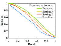
(b)

Figure 4: (a) ROC curve and (b) precision-recall curve of NN ensembles with different settings (all testing samples included).

VI-B NN Ensemble vs. RF

For comparison, we also list the performance with RF in Table III, which is configured as having 100 voters, each using at most 20 (raw) features. The bold font indicates that RF performs better than the proposed NN ensemble (setting 4). Comparing the columns of “setting 4” and “RF” in Table III, we can see the proposed NN ensemble model achieves similar, if not better, performance to that of RF in terms of effective accuracy, areas under ROC curve and precision-recall curve. At least half of test sets shows better performance in terms of any metric (e.g., 8 out of 12 test sets have better $A_{roc}$) using the proposed model than RF. Therefore, the proposed model can be used as a good complement to RF.

VII Conclusions

In this paper, we use NN ensembles to predict DRC hotspot in early stages of physical design. With a systematic feature subset selection scheme, the performance of the proposed model is significantly improved over a single NN, and is better or comparable to that of RF. The proposed NN ensemble model can be easily implemented with popular NN frameworks with affordable computational cost.

References

- [1] A. F. Tabrizi et al., “A machine learning framework to identify detailed routing short violations from a placed netlist,” in DAC, 2018.
- [2] A. F. Tabrizi, N. K. Darav, L. Rakai, A. Kennings, and L. Behjat, “Detailed routing violation prediction during placement using machine learning,” in VLSI-DAT, 2017.
- [3] W.-T. J. Chan, P.-H. Ho, A. B. Kahng, and P. Saxena, “Routability optimization for industrial designs at sub-14nm process nodes using machine learning,” in ISPD, 2017.
- [4] L. K. Hansen and P. Salamon, “Neural network ensembles,” IEEE Trans. Pattern Anal. Mach. Intell., vol. 12, no. 10, pp. 993–1001, 1990.
- [5] A. Krogh and J. Vedelsby, “Neural network ensembles, cross validation, and active learning,” in NIPS, 1995.
- [6] Z.-H. Zhou, J. Wu, and W. Tang, “Ensembling neural networks: many could be better than all,” Artif. Intell., vol. 137, no. 1, pp. 239–263, 2002.
- [7] I. Jolliffe, “Principal component analysis,” in Int’l Encyclopedia of Statistical Science. Springer, 2011, pp. 1094–1096.
- [8] F. Z. Brill, D. E. Brown, and W. N. Martin, “Fast generic selection of features for neural network classifiers,” IEEE Trans. Neural Netw., vol. 3, no. 2, pp. 324–328, 1992.
- [9] D. W. Opitz, “Feature selection for ensembles,” in AAAI/IAAI, 1999.
- [10] H. D. Navone, P. F. Verdes, P. M. Granitto, and H. A. Ceccatto, “Selecting diverse members of neural network ensembles,” in Proc. Brazilian Symp. on Neural Networks, 2000.
- [11] J. Che, Q. Wu, and H. Dong, “A random feature selection approach for neural network ensembles: Considering diversity,” in Int’l Conf. on Computational Intelligence and Software Engineering, 2010.
- [12] M. Abadi et al., “Tensorflow: Large-scale machine learning on heterogeneous distributed systems,” arXiv:1603.04467 [cs.DC], 2016.
- [13] F. Chollet et al., “Keras,” https://keras.io, 2015.
- [14] I. S. Bustany, D. Chinnery, J. R. Shinnerl, and V. Yutsis, “ISPD 2015 benchmarks with fence regions and routing blockages for detailed-routing-driven placement,” in ISPD, 2015.
- [15] T. K. Ho, “Random decision forests,” in Int’l Conf. on Document Analysis and Recognition, vol. 1, 1995.
- [16] N. K. Darav, A. Kennings, A. F. Tabrizi, D. Westwick, and L. Behjat, “Eh?placer: a high-performance modern technology-driven placer,” TODAES, vol. 21, no. 3, art. 37, 2016.
- [17] Mentor Graphics Inc., “Olympus-SoC,” https://www.mentor.com/products/ic_nanometer_design/place-route/olympus-soc/. [08-25-2018].
- [18] C.-K. Wang et al., “Closing the gap between global and detailed placement: Techniques for improving routability,” in ISPD, 2015.
- [19] L.-C. Chen, C.-C. Huang, Y.-L. Chang, and H.-M. Chen, “A learning-based methodology for routability prediction in placement,” in VLSI-DAT, 2018.
- [20] Q. Zhou, et al., “An accurate detailed routing routability prediction model in placement,” in ASQED, 2015.
- [21] W.-T. J. Chan, Y. Du, A. B. Kahng, S. Nath, and K. Samadi, “BEOL stack-aware routability prediction from placement using data mining techniques,” in ICCD, 2016.
- [22] Y. Wei et al., “Glare: Global and local wiring aware routability evaluation,” in DAC, 2012.
- [23] D. P. Kingma and J. Ba, “Adam: A method for stochastic optimization,” arXiv:1412.6980 [cs.LG], 2014.