Median Confidence Regions in a Nonparametric Model
Abstract
The nonparametric measurement error model (NMEM) has where is the class of all continuous distributions with median , so is the median parameter of . This paper deals with the problem of constructing a confidence region (CR) for under the NMEM. This problem arises in many settings, including inference about the median lifetime of a complex system arising in engineering, reliability, biomedical, and public health settings. Current methods of constructing CRs for are discussed, including the -statistic based CR and the Wilcoxon signed-rank statistic based CR, arguably the two default methods in applied work when a confidence interval about the center of a distribution is desired. Optimal equivariant CRs are developed with focus on subclasses of when looking at their expected Lebesgue content. Applications to a real car mileage efficiency data set and Proschan’s air-conditioning data set are demonstrated. Simulation studies to compare the performances of the different CR methods were undertaken. Results of these studies indicate that the sign-statistic based CR and the optimal CR focused on symmetric distributions satisfy the confidence level requirement, though they tended to have higher contents; while two of the bootstrap-based CR procedures and one of the developed adaptive CR tended to be a tad more liberal but with smaller contents. A critical recommendation is that, under the NMEM, both the -statistic based and Wilcoxon signed-rank statistic based confidence regions should not be used since they have degraded confidence levels and/or inflated contents.
Key Words and Phrases: Bootstrap confidence region; BCa confidence region; Confidence region; Content of a confidence region; Equivariant confidence region; Expected values of differences of order statistics; Invariant models; nonparametric confidence region; nonparametric measurement error model.
2010 AMS Subject Classification: Primary: 62G15; Secondary: 62G09, 62G35.
1 Introduction and Motivation
Given a univariate distribution function , the two most common measures of central tendency are the mean , provided it exists (), and the median . The mean need not always exist, whereas the median always exists. Under symmetric distributions, and when the mean exists, then the mean and the median coincide. This paper is concerned with making statistical inferences about the median of a distribution. A popular model leading to the problem of making inference about the median of a distribution is the so-called measurement error model. In this model represents a quantity of interest which is unknown, and when one measures its value, the observed value is a realization of the random variable
| (1) |
where represents a measurement error with a continuous distribution whose median equals zero. As such, the distribution of is . Typically, is assumed to be a zero-mean normal distribution, but this assumption is not tenable in many situations. For instance, in dealing with event times in biomedical, reliability, engineering, economic, and social settings, the error distribution need not even be symmetric. This is also the case when dealing with economic indicators such as per capita income, retirement savings, etc. As such, a general model is to simply assume that the error distribution belongs to the class of all continuous distributions with medians equal to zero. This class will be denoted by .
Another situation where this problem arises is when dealing with a complex engineering system, such as the motherboard of a laptop computer or some technologically-advanced car (e.g., a Tesla Model S sedan). Such a system will be composed of many different components configured according to some structure function, with the components having different failure-time distributions and some of them possibly acting dependently on each other. Of main interest for such a system will be its time-to-failure (also called lifetime) denoted by . Because of the complexity of the system, it may not be feasible to analyze the distribution of by taking into account each of the failure time distributions of the components and the system’s structure function which represents the configuration of the components to form the system. Thus a simplified and practically feasible viewpoint is to assume that the system’s life distribution is some continuous distribution . One may then be interested in the median of this distribution .
Thus, in these situations, the observable random variable is assumed to have a distribution with and being the median of . This will be referred to as the one-population nonparametric measurement error model, abbreviated NMEM. This is the simplest among the measurement error models. The goal is to infer about the parameter of interest with acting as an infinite-dimensional nuisance parameter. We shall be interested in this paper in the construction of a confidence region (CR) for based on a random sample of observations of . This definitely is a classic problem since the construction of a confidence interval for the median was even discussed in ([14]). More generally, quantiles instead of just the median may be of interest, and the methods developed here could be adaptable to inference about general quantiles.
Arguably, confidence regions for a parameter are preferable than point estimates since they address simultaneously the issue of how close to the truth (measured through the content of the region) and how sure about such closeness to the truth (measured by the confidence region coefficient). For more discussions on desirability of confidence regions see, for instance, the introduction in [3] and chapter 5 in [2]. Of course, one could typically accompany a point estimate (PE) by an estimate of its standard error (ESE), but then the user still needs to deduce closeness and sureness based on the PE and the ESE, usually a non-trivial matter if to be done properly.
We introduce some notations and definitions. Let be independent and identically distributed (IID) random variables (a random sample) from , where and . The mathematical problem is to construct a confidence region (CR) for the parameter with an infinite-dimensional nuisance parameter. Denote by the range space of which will be endowed with a -field . We also denote by the Borel -field of , and this will be endowed with the -field of subsets of consisting of its countable and co-countable subsets, with this -field denoted by .
Definition 1
Fix an . Let be IID from . A measurable mapping is called a region estimator or confidence region (CR) for if for every .
Remark: In later developments, we will allow the CR to also depend on a randomizer , a standard uniform random variable independent of . This is to be able to achieve exactly the desired confidence level . In such a case, and will be the realized CR when and . However, even if we allow for randomized CRs, we will usually suppress writing the in and simply write .
Aside from satisfying the desired confidence coefficient in Definition 1, the quality of a CR depends on some measure of its content. Let be Lebesgue measure on . We will measure the content of a CR for via
| (2) |
In Definition 2 below we have the notion of uniformly best CRs. Our goal is to determine those CRs for that possess such optimality properties.
Definition 2
Let be a subclass of . A CR for is a uniformly best CR for under the subclass if for any other CR ,
for all . If , then will be said to be the uniformly best CR for .
The major contribution of this work is the development of randomized region estimators or confidence regions, possibly approximate, for the median under the NMEM, of form
where and is an appropriate estimator of . The randomizer is a uniform random variable, while is the infimum over all satisfying where is a binomial random variable with parameters and . A specific form of that leads to a reasonable CR is given by
where , the empirical distribution function of , with being the sample median. The specific CR above will be developed in section 5. Prior to the development of the specific CRs, in section 2 we utilize invariance ideas to derive the general form of the almost-optimal equivariant CR for under the NMEM but still under the assumption that is known. Then, we address the question of how to deal with the fact that is not actually known, leading to the region estimator above. Two other region estimators which are focused toward the class of symmetric distributions and the class of negative exponential distributions, but still valid for the general NMEM model, will be developed in sections 3 and 4, respectively. In the simulation studies, the procedure focused on symmetric distributions actually performed quite robustly under varied distributions (even for the non-symmetric distributions) in terms of coverage probability and it had mean content superior to the procedure based on the sign statistic. Prior to studying the performance of these new region estimators, we briefly describe existing (‘off-the-shelf’) region estimators for the median in section 6. We then proceed to demonstrate these different region estimators by applying to two data sets in section 7. Section 8 will present the results of simulation studies comparing the performances of these region estimators under different underlying distributions by examining their mean contents and their achieved confidence levels. These comparisons are also of major importance since they demonstrate CR procedures that should be preferred and which CRs should not be used under the NMEM . Section 9 will provide some concluding remarks.
2 Development of Optimal CRs
2.1 Invariant Models and Equivariant CRs
We first review the notions of invariant statistical models and equivariant CRs (see, for instance, [9]). We do this review in a more general framework than the concrete NMEM which is the focus of this paper. We note that sufficiency and invariance were major ideas utilized by Peter Hooper in several of his papers dealing with confidence sets and prediction sets, cf., [7, 6, 8].
Let be an observable random element taking values in a sample space . The class of probability models governing is which consists of probability measures ’s on the measurable space , with a suitable -field of subsets of . Let be a functional, with being the parameter of interest. A confidence region for is a set-valued mapping , where is a class of subsets of such that
| (3) |
Let be a family of transformations on that forms a group under an operation and with identity element . Let be a group of transformations on such that there exists a homomorphism and let be the identity element in . The statistical model is said to be -invariant if
| (4) |
In addition, let be a group of transformations on such that there exists a homomorphism . The parametric functional is said to be -equivariant if for all . Employing a decision-theoretic framework, define a loss function on given by the loss function
We shall say the the loss function is -invariant if for every , , and . Given a confidence region , its risk function is
As such, the condition for a confidence region is equivalent to having for every . When a -invariant statistical model is coupled with a -invariant loss function, then we would say that the statistical problem of constructing a confidence region is -invariant. A confidence region is then said to be -equivariant if for every and , we have that
The Principle of Invariance then dictates that we should only utilize -equivariant confidence regions.
For an invariant confidence region problem, if is equivariant, then we have that, for every ,
Furthermore, if the group is transitive over , meaning that for any given we have , then it suffices to consider an arbitrary element to determine for all since this equals the value using the arbitrary .
Recall that we also need to measure the quality of a confidence region by measuring its content using the quantity where is a measure on , e.g., Lebesgue measure. We seek those confidence regions with small . Observe that for an equivariant in an invariant statistical model, we have for every that
If it so happens that for all and and for some , then there is the possibility of finding a that satisfies the required confidence level and minimizes the content. We shall call this condition as quasi-invariance of with respect to . However, if -quasi-invariance of does not hold, then a uniformly best confidence region may not exist. But, a uniformly best confidence region on a subfamily may still exist among the class of confidence regions over . In [7, 6] quasi-invariance of the measure was imposed, but in some settings this may be unnatural such as in the NMEM under consideration in the current paper.
2.2 Towards Optimal CRs for the Median
Consider now the problem of constructing a CR for the median under the NMEM: Prior to invoking invariance, we first reduce via the Sufficiency Principle. Thus, we may assume that the observable random vector is , the vector of order statistics which is a complete sufficient statistic. The appropriate sample space is therefore . A word on our notation: even though we had reduced to , in the sequel, when we write or , this means that the common distribution of the original ’s is . For measuring the content of a region for we use Lebesgue measure on .
The first invariance reduction is obtained through location-invariance. The problem is invariant with respect to translations with the groups of transformations being, for every ,
A CR is location-equivariant if, for every , where . Observe that for a location-equivariant , we have for every that
by taking to obtain the last equality. The problem has thus been reduced to considering to be the order statistics from and we seek a location-equivariant such that, for every , In addition, we seek to minimize over all . Note that Lebesgue measure in is location-invariant, that is, for every and .
We remark at this stage that if we know the distribution , then we could determine the optimal CR for under this known distribution and no further invariance reduction will be needed. To demonstrate, suppose that is the normal distribution with mean zero and variance which could be taken to be , so , with the standard normal distribution function (we also let to denote the standard normal density function). Then, we seek a location-equivariant satisfying and with minimized. Under , the joint density function of is given by . Thus, we want On the other hand, we obtain
where
obtained after the obvious change-of-variables. The problem is then to find a location-equivariant that will minimize subject to the condition that The solution to this constrained minimization problem (see the optimization result in Theorem 2) is the well-known -confidence interval for the normal mean given by
However, since is known only to belong to , a further invariance reduction is needed. This is achieved through strictly increasing continuous transformations with as a fixed point. Let denote the collection of functions that are strictly increasing continuous function on with . The groups of transformations are given by
is then equivariant with respect to these groups of transformations if
so that for every and , we have We then have that, for every and ,
Observe, however, that
and we do not have in this situation quasi-invariance of the measure with respect to the groups of monotone transformations.
The group of transformations with is transitive over . Thus, we may simply pick an arbitrary , which could be taken to be , the uniform distribution over . Indeed, if , then with , we have . Thus,
We emphasize again that in the second equation we could not drop the term nor factor it out from inside the measure. This will prevent us from obtaining a uniformly (over ) best confidence region for .
Next, we obtain a representation of by choosing a specific member of that depends on . For an , define for via
and for define it such that it is strictly increasing and continuous over all . Observe that for ,
where . Note that and observe that
Lemma 1
With defined as above, a location-equivariant (LE) and -equivariant (ME) has representation
| (5) |
where is some region in . Thus, the LE and ME ’s are determined by ’s, which are subsets of . In fact, given a , we have
| (6) |
whose Lebesgue measure is
2.3 Optimal CRs
Next, we tackle the problem of choosing an ‘optimal’ (properly defined) region , which then determines via the representation in Lemma 1. Recall that the goal is to find such that with , and, for every , minimized, or if this is not possible, made small. Note that under , has a binomial distribution with parameters , denoted by , and with associated probability mass function We have that
with the first equality obtained using the portion of the proof of Lemma 1 and where we define The expected Lebesgue measure of is
where, with and ,
| (7) |
Assume first that we know the values of . We now allow for randomized confidence regions in order to achieve optimality, that is, we allow for and to depend on a randomizer which is a standard uniform random variable independent of the ’s. We remark that in [7, 6, 8] randomized procedures were also allowed to enable achieving optimality, similarly to the Neyman-Pearson theory of most powerful tests (cf., [9]).
Define the right-continuous non-decreasing -valued function, for ,
For a given , define
Define the function over via
The optimal then satisfies
Theorem 2
Let and let be as defined in (7). Then Furthermore, if is any other -valued function in with then
where the expectation is with respect to the randomizer .
Proof: From the form of , we have
Let be any other function on with From the definition of , we observe that for each ,
Summing over and integrating over , we find that
Since and by condition we have , then
which completes the proof of the theorem.
Remark: We note that this proof is similar to that of the Neyman-Pearson Lemma except for the fact that the is not a distribution function.
Therefore, the optimal , possibly using a randomizer , is
The associated optimal confidence region for , possibly randomized, is
| (8) | |||||
Note that if we drop the term in bracket containing in (8), we obtain
| (9) |
which is a conservative confidence region for in the sense that If is a natural confidence coefficient (cf., [13]) associated with the binomial distribution, then we may still obtain an exact confidence region.
2.4 Implementation Aspects
The optimal confidence region required knowledge of the ’s, or at the very least the ordering of the for inclusion in the , which is determined by the magnitude of the ratios . In general, will depend on the unknown true distribution , hence the values of ’s or the ’s will not be known. In this case, we will not be able to determine . We describe two approaches to circumvent this problem.
-
(i)
Restrict to belong to a subclass of the family of continuous distributions, say and determine the ’s or the ’s for this class. This is then tantamount to satisfying the confidence level condition over the whole of , but focusing only on the subclass for minimizing the expected Lebesgue measure of the confidence region.
-
(ii)
Utilize the observed data to estimate by , then use these ’s in the expression of . There are several ways to accomplish this which are discussed below. However, it should be pointed out that when estimates are plugged-in, data double-dipping ensues and the achieved confidence level may not anymore satisfy the condition of being at least equal to .
The next two sections will deal with these two approaches towards developing the region estimators.
3 Optimal CRs Focused on Symmetric Distributions
3.1 For Uniform Distributions
We illustrate the different approaches for dealing with the situation of unknown . Let us consider approach (i) first. Suppose that we consider the subfamily of uniform distributions. It suffices to consider for . Note that iff with . Thus, and it is well-known that . As such , hence
Consequently, the ratios of interest are
Hence, the optimal is of form where is the smallest value such that . Since the mapping from into is symmetric about and decreases as increases, then for satisfying
This implies that is the th quantile of , denoted by , obtainable via the qbinom function in R ([12]). Letting and , then
With
the resulting randomized confidence region for is
| (10) |
This CR procedure is the randomized version of the sign-statistic based CR, given in (13) and denoted by . This CR was the confidence interval developed in [14].
3.2 For General Symmetric Distributions
We assumed the uniform family of distributions in the preceding subsection. A question arises whether we obtain the same CR if belongs to the subfamily of , the additional condition being symmetry of the distribution. For instance, the classes of normal, Cauchy, logistic, double exponential, symmetric mixtures of distributions all belong to this subclass. It turns out that is also optimal for this larger subclass as a consequence of Theorem 3. The CR based on the Wilcoxon signed-rank statistic is an appropriate CR for these symmetric class of continuous distributions; however, this CR is not a legitimate competitor of since it does not satisfy the confidence level requirement for non-symmetric distributions which are still under the NMEM.
Theorem 3
Let be IID from and define , with and . Let
-
(i)
If is even, then is maximized at and it decreases from the maximum as increases.
-
(ii)
If is odd, then is maximized at and decreases when increases for or when increases for .
The results stated in Theorem 3 appear intuitive when the distribution is unimodal. What is surprising is that the results also hold when is bi-modal or multi-modal. For instance, if we take a symmetric mixture of a and a , even when is quite large relative to , the results still hold true. We present a mathematical proof of Theorem 3. To do so we first establish an identity analogous to that given by Pearson in a paper of [5].
Lemma 4
Let be the associated order statistics for a random sample of size from a continuous distribution . For , and provided that the expectations are well-defined with possibly a value of , then
Proof: Recall that for a positive-valued continuous random variable , we have , hence for a general continuous ,
For , we also recall that . Using these expressions, we immediately find that
We now prove Theorem 3.
Proof: Using the representation in Lemma 4, we have for that
Let . We prove the results by showing that is symmetric about and that it first decreases then increases with the maximum occurring at values of that depends on whether is odd or even. Making the transformation in the expression of and denoting by the density function of , we have
In the last integral, let and note that since , so that . Consequently,
Letting and , it follows that
In the last integral, all terms in the integrand outside the brackets are nonnegative. Let for For this function, we have
In addition, we have
Therefore, on , is decreasing when ; constant at when ; and increasing when . Consequently,
This completes the proof of the theorem.
4 Optimal CRs Focused on Exponential Distributions
Next, we consider the situation where the focused class of distributions is the negative exponential familiy, a right-skewed class of distributions, in contrast to the symmetric distributions considered above. Let be IID from an exponential distribution (Exp()) so the common median is . From the normalized spacings theory (see, for instance, [1]) we have that
where are the normalized spacings statistics, which are also IID from Exp(). As such, with , we obtain
It follows that under this negative exponential distribution model,
The optimal will therefore be of form
with chosen to be the smallest value such that Note that this subset will never include , but it could include . We shall denote by the resulting randomized CR for under this exponentially-distributed focused case.
We illustrate the resulting CR for concrete values of . We start with , an even sample size. Using R [12] we obtain for each the values of (up to proportionality) and given in Table 1.
| 0 | 1 | 0.0009765625 |
| 1 | 9 | 0.0097656250 |
| 2 | 36 | 0.0439453125 |
| 3 | 84 | 0.1171875000 |
| 4 | 126 | 0.2050781250 |
| 5 | 126 | 0.2460937500 |
| 6 | 84 | 0.2050781250 |
| 7 | 36 | 0.1171875000 |
| 8 | 9 | 0.0439453125 |
| 9 | 1 | 0.0097656250 |
| 10 | 0 | 0.0009765625 |
Observe that the way we start including values of into is according to the value of . Thus we start by first including -values of 4 and 5; then 3 and 6; etc. Observe the asymmetry in the process of including the -values into with a bias in favor of the lower -values. The intuition behind this is that since the exponential distribution is highly right-skewed, then the expected lengths between successive order statistics increases as increases, which is formally indicated by the expression. Thus, to shorten the interval, there is preference for the lower order statistics. For a 95% confidence region, from the table we find that which yields . The randomization probability then becomes
The 95% (randomized) confidence region for the median will then be
When , an odd sample size, by following the same calculations as for and with the first -value to enter being , we find the 95% (randomized) confidence region for the median to be
5 Data-Adaptive Methods
Next we demonstrate approach (ii). In this situation we do not know the ’s so we instead estimate these quantities using the observed data. Recall that so that without any knowledge about the underlying we will not have a closed-form expression for these ’s. However, given the sample data, we could estimate , unbiasedly, by
which is the method-of-moments estimator. This estimator though maybe unstable or inefficient. Using this estimator, we may then order the in terms of priority of entry into according to the quantities
As such the form of the ‘optimal’ will be
We shall denote by the resulting randomized CR. The constant will be chosen to be the smallest value such that . This value of will depend on the sample data since the ordering of entry of the -values into will depend on , so that the randomization probability will also depend on . Because of this dependence of the and values to the sample data , it is possible that the achieved confidence coefficient of the resulting confidence region will not anymore be . In the simulation studies in section 8 we will indeed see that there is degradation in terms of the achieved confidence level for this CR.
A possibly better adaptive approach is to utilize the representation of in Lemma 4 and to replace the unknown in the expression by an estimator based on the , where is the sample median of the ’s. We expect this will lead to a better procedure since the estimators of the ’s will be more stable compared to the method-of-moments estimator discussed above. In our implementation of this idea, we use as our estimator of the empirical distribution function of , given by The resulting estimator of is then
Observe that we could also just have used the EDF of the ’s instead of the ’s since the cancel out. As such, to order the in terms of entry into , we use
The resulting randomized CR for will be denoted by .
These adaptive procedures are totally nonparametric in the sense that no knowledge of the underlying distribution is required. If we do have knowledge of the families of distributions in which belongs, then we may be able to provide a better estimate of the ’s as in the preceding subsection. It should also be noted, however, that these adaptive procedures may not anymore satisfy the confidence level requirement due to the data-dependent plug-in step. Section 8, which presents results of simulation studies, provides some insights regarding the empirical properties of these procedures.
6 Brief Review of Existing ‘Off-the-Shelf’ Median CRs
There are several existing methods for constructing frequentist-based CRs for under the NMEM. We describe some of these methods prior to our illustrations and simulation studies. For a sample realization , we define the usual sample statistics:
, , , and will then represent the random versions of these sample statistics. As earlier mentioned, and will be the standard normal density and distribution functions, respectively, the standard normal quantile function. We will use the conventional notation for the th quantile of . and will denote the distribution and quantile functions, respectively, of a Student’s random variable with degrees-of-freedom , and its th quantile will be denoted by .
Arguably, the most commonly-used CR for the center of a distribution, which is for symmetric distributions, is the -based CR given by
| (11) |
However, this CR is actually not valid under the NMEM since it does not satisfy the condition for all . We still included this CR since it is typically the first choice to use by practitioners when constructing a confidence interval for or and we would like to examine and compare its performance with other CRs under the NMEM.
The nonparametric analog of the -based CR is the CR constructed from the Wilcoxon signed-rank statistic ([13]). The Walsh averages associated with the sample ’s are for . Let be the order statistics of these Walsh averages. This Wilcoxon signed-rank based nonparametric CR is given by
| (12) |
where, with denoting the null distribution (that is, under and ) of ,
This CR is valid under , but not for . In contrast, the nonparametric CR derived from the sign statistic is valid under (see [14]). As before, let be the binomial distribution with parameters and . Let
Then, this sign statistic-based CR is
| (13) |
Another CR of is developed from the asymptotic normality of the sample median . For IID from a distribution with density , this asymptotic distribution (cf., [13]) is given by
If is an estimator of , then an asymptotic confidence interval for is
| (14) |
Kernel-based estimators of the density are available in R using the density object function ([12]), and coupled with the approx function, could then be estimated. This is how we implemented this CR in the illustrations and in the simulation studies.
Instead of relying on asymptotic approximations, one may resort to bootstrapping approaches. Let be the th bootstrap sample out of BREPS bootstrap samples. Denote its sample median by . The basic bootstrap CR using the median obtains the th and th quantiles of , denoted by and , respectively, and constructs the CR (cf., [4]) via
| (15) |
The next bootstrapped CR is derived using the studentized median as pivot and with its standard error estimated by , the standard deviation of . The CR is constructed via
| (16) |
The bootstrap percentile CR also uses the bootstrap distribution of . Denoting by
the (empirical) bootstrap distribution, the percentile bootstrap CR is
| (17) |
where is the bootstrap quantile function.
This percentile bootstrap CR is usually bettered by so-called bias-corrected CRs. See, for instance, chapter 5 of [2] and chapter 11 of [4]. The first improvement is provided by the bias-corrected (BC) CR which is
| (18) |
where and . On the other hand, the BCa method (bias-corrected and accelerated) CR takes the form
| (19) | |||||
where the acceleration coefficient can be estimated using jackknifed samples estimates via
with with the sample median of the th jackknifed sample
Together with these existing CRs for , we add the CRs developed in earlier sections (we drop the superscript ‘∗’ in the notation): , the CR optimized for symmetric distributions [see equation (10)]; , the CR optimized for exponential distributions (see section 4); , the adaptive CR using the crude estimator for ; and , the adaptive CR using the empirical distribution in the estimator of (see section 5). We summarize these different CR procedures examined in the illustrations and the simulation studies in Table 2. We note that among these thirteen CRs, those that are location-equivariant and equivariant to monotone transformations are , , , , and .
| Method Label | Description or Type or Basis of CR |
|---|---|
| Statistic Based | |
| Wilcoxon Signed-Rank Statistic Based | |
| Sign Statistic Based | |
| Asymptotic Distribution of Median Based | |
| Basic Median Bootstrap | |
| Median with Bootstrapped SE | |
| Percentile Bootstrapped | |
| Bias-Corrected (BC) Bootstrapped | |
| Bias-Corrected Accelerated (BCa) Bootstrapped | |
| Optimally Focused for Symmetric | |
| Optimally Focused for Exponential | |
| Adaptive with Unbiasedly Estimated | |
| Adaptive with Estimated using EDF |
7 Illustration using Real Data Sets
For our first illustration we use a real data set gathered by the first author about the mileage efficiency of his car during a period when he was commuting between Ann Arbor, Michigan and Bowling Green, Ohio. Efficiency is measured in terms of the miles traveled per gallon of gasoline. In the data set there were observations, with each observation recorded at each gas fill-up. The histogram of these observations are shown in Figure 1. The full data set, which contained other relevant variables, was also used in demonstrating linear model global model validation procedures in [10].
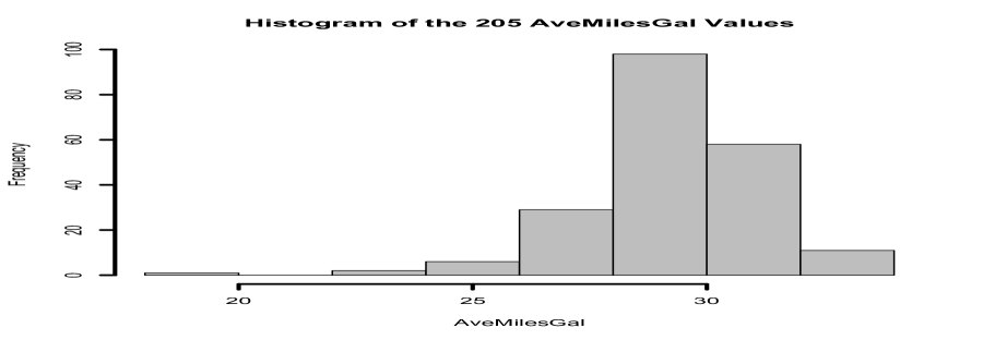
For this sample data the sample mean is , sample median is , the first and third sample quartiles are 28.275 and 30.575, respectively, and the extreme values are 18.374 and 33.472. From the histogram we notice that there is a noticeable left-skewness in the distribution. The sample standard deviation is 1.887 and the inter-quartile range is 2.299. For our illustration, we seek a confidence region for the population median , where the population could be thought of as the hypothetical set of all values of AveMilesGal if the car has been observed forever. We mention that one interesting aspect of this data set is that the population from which this sample is obtained is a mixture of subpopulations corresponding to summer highway driving, winter highway driving, summer city driving, winter city driving, and a combination of highway and city driving.
Figure 2 depicts the 95% confidence regions produced by the thirteen different methods for the AveMilesGal data set.
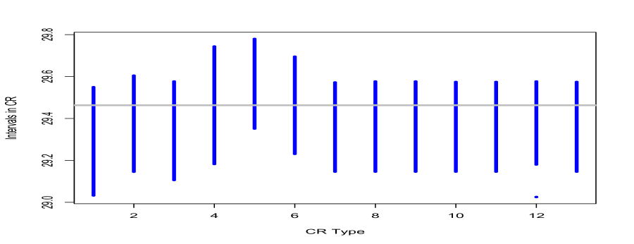
Except for CR , all of them produced intervals. It is possible that method may also produce a region that is not an interval, while CRs to will all produce confidence intervals by construction. In addition, observe that only the CRs produced by and turned out to be symmetric about the sample median.
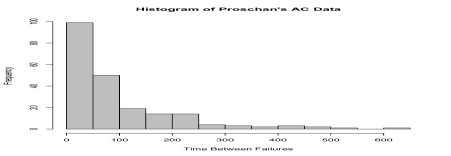
provides a histogram of the 212 observations in this data set, with each observation being a time between successive failures. To un-tie tied observations (we perturb the original values in tied sets of observations by uniform variates over . Note the high right-skewness of this data set. Proschan also demonstrated that this data set did not come from an exponential distribution, but came from a mixture of exponential distributions, inducing a decreasing failure rate property. Our goal in this illustration is to provide a confidence region for the median inter-failure time given this data set. Figure 4
presents the comparative plots of the CRs for the thirteen methods. Notice that the -based CR, as well as the Wilcoxon signed-rank based CR, appear to be rather different from the other eleven CRs. In fact, both excluded the sample median. At the same time, we are somewhat unfair in the manner in which we applied these two procedures since it would have been more appropriate to first perform a transformation to approximately symmetrize the distribution prior to applying these procedures, and then re-transforming back. Also, notice that the CR is composed of one big interval together with several smaller intervals. This could be attributed to the instability of the method-of-moments estimates of the ’s. Interestingly, this CR has the smallest content, but we will see in the simulation studies in section 8 that its achieved coverage probability of the median tends to be lower than the nominal coverage probability.
8 Comparison of Methods via Simulations
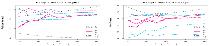
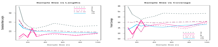
In this section we present the results of simulation studies to compare the thirteen CR methods listed in Table 2 in terms of their contents and coverage probabilities under the NMEM. Different error distributions [normal, Cauchy, uniform, logistic, gamma, Weibull and mixture of normals] and varied sample sizes () were utilized in the simulations. The computer programs were coded in R [12]. For each combination of error distribution and sample size, 10000 simulation replications were ran, and with 2000 bootstrap replications for the bootstrap-based methods.
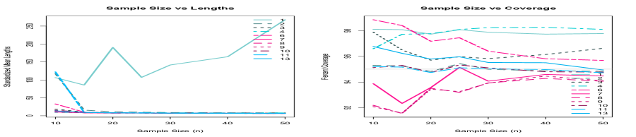
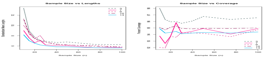
Figures 5 and 6 present the results of this simulation study in the form of plots of the standardized mean contents (these are the simulated mean contents multiplied by the square root of the sample size) and the percentage coverage of the true median under different distributions and for the varied sample sizes. As we progress with the different distributions we eliminated in the plots the methods that were not competitive, either with respect to their achieved coverage probability or their mean content. This is in order to make the plots leaner and cleaner and to enable more clear-cut comparisons among those methods that are competitive. Methods that were eliminated from contention after a distribution run are as follows (they were still included in the runs but eliminated only in the plots): normal [5, 12 due to coverage]; Cauchy [1 due to content]; uniform [4 due to coverage]; logistic [none]; gamma [2 due to coverage]; Weibull [8 since almost the same as 9]; normal mixture [6 due to coverage]. Upon final examination of the resulting plots we also eliminated method 11 since it is unstable with respect to content.
The first observation from these simulations concerns the performance of and . Both perform very well under the normal distribution with having smaller content as expected, but performs extremely poorly with respect to content under the Cauchy distribution, and both do not perform well in terms of coverage for non-symmetric distributions. However, their poor performances under non-symmetric distributions are also expected. The next observation is the consistent validity of the sign-statistic based procedure . Its coverage probability is always at least the specified coverage probability and in fact it tends to be conservative. At the same time, it has the highest mean content among the competitive methods. , which is the procedure focused towards symmetric distributions and which is actually a randomized version of , is preferable over since it has smaller mean content and at the same time it satisfies the coverage requirement. The basic bootstrap CR, , surprisingly performed poorly with respect to its achieved coverage probability. The CR based on the studentized sample median using a bootstrapped standard deviation as estimate of the median’s standard error, , did not perform well for small sample sizes in terms of coverage probability. and almost have the same performance, as is to be expected from their derivations, while tended to have unstable mean contents. did not perform acceptably due to its degraded coverage probability. Thus, based on these simulation studies, the most competitive among the thirteen CR procedures are , , , , and .
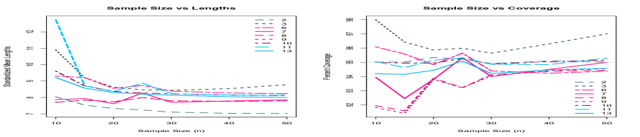
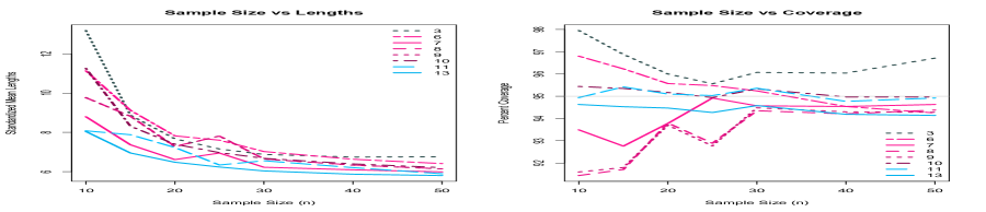
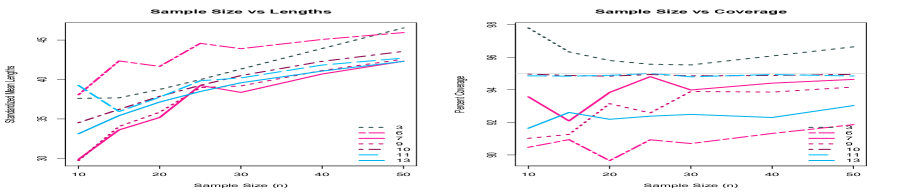
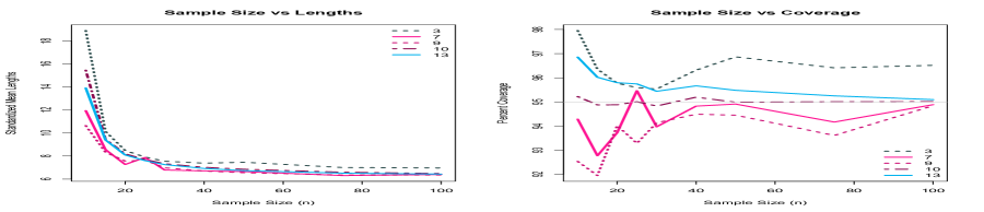
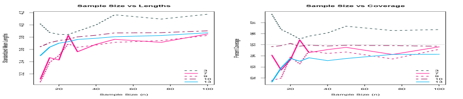
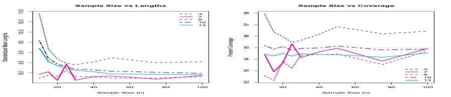
To focus comparisons among these five procedures, we ran more extensive simulations with 20000 replications and 5000 bootstrap replications for sample sizes to obtain better comparisons of these five chosen methods. The results of these simulations are contained in Figures 7 and 8. Examining the plots in Figures 7 and 8, we see that the sign-based test, , and the procedure focused on symmetric distributions, , are consistently satisfying the confidence level requirement among all the distributions considered, including the skewed gamma and Weibull distributions, with tending to be more conservative. , which as pointed out earlier is a randomized version of , has confidence level that is very close to the pre-specified level, hence it also has smaller content compared to . The PCT-Bootstrap, , and the BCa-Bootstrap, , tend to be liberal, and so is the adaptive , though the latter could sometimes be conservative such when the distribution is Cauchy, or it could be more liberal than and such as for the mixture of normal distributions. Content-wise, , , and almost have the same performances, with appearing to be having a tad smaller content. Due to the lower achieved confidence, these three CRs also tended to have smaller contents compared to and , with possessing the largest content and being also the most conservative. We note here the impact of the plug-in procedure for . Since we did not know we plugged-in an estimator for this function which utilized the empirical distribution function and which also used the same sample data, so there is data double-dipping. The impact of this plug-in and double-dipping procedure is to make the procedure somewhat liberal. In contrast, the CR did not need this plug-in procedure and we observe that the achieved level for this CR is very close to the pre-specified confidence level.
9 Concluding Remarks
In this paper we revisit the problem of constructing confidence regions (CRs) for the median under the NMEM. The problem is also relevant in the study of complex engineering systems where it is difficult to determine the exact functional form of the system’s lifetime distribution, so one is forced to utilize a nonparametric model for the system’s lifetime distribution. In addition, this problem also arises in economic settings where of interest will be the median instead of the mean when dealing with the income variable due to high right-skewness of its distribution. Several existing nonparametric approaches to constructing CRs for the median were reviewed. Among these ‘off-the-shelf’ methods are the -based method which utilizes the sample mean, and that based on the Wilcoxon signed-rank statistic. These two methods may perhaps be the default methods for many users whose goal is to infer about the ‘center’ of the population distribution. Also included are the computationally-intensive CR methods such as the bootstrap percentile and the BCa approaches ([4]).
When assessing the adequacy of a CR, there is a need to examine its expected content (in one-dimensional settings, content is its Lebesgue measure) in addition to the requirement that it satisfies a specified nominal level of coverage of the true parameter value. Thus we examined the problem of obtaining optimal CRs, which are those with smallest expected contents. Under the NMEM, invariance with respect to location-shifts and monotone transformations were invoked to reduce the problem to constructing equivariant CRs. Within the class of equivariant CRs, we obtained the best CRs, with respect to minimizing the expected content for subclasses of the class of all continuous distribution functions. Thus, there is a best CR when focused on the subclass of symmetric distributions and a best CR for the subclass of exponential distributions. We also developed fully nonparametric data-adaptive CRs under the NMEM. These adaptive CRs are the ones labeled and . Based on simulation studies to compare the different CRs, we found that under the NMEM, both the -based and the Wilcoxon signed-rank statistic based CRs should not be utilized. The sign-statistic based procedure, , and the optimal procedure focused towards symmetric distributions, , both fulfill the confidence level requirement, with being somewhat conservative, hence tended to have larger content. Among the other CR methods, the bootstrap procedures (PCT) and (BCa), and the adaptive procedure , were the most competitive among all scenarios, but these three tended to be a tad more liberal than either and , hence also possessed smaller contents. If one is to insist that the desired confidence level should be achieved, then appears to be the best, or if one is opposed to using randomized CRs, then should be chosen. However, we feel that abhorrence to the use of randomized procedures is not mathematically justifiable nor defensible, since the use of randomized procedures allows for better methods and such strategies are in fact the bulwark of statistical decision and game theory. On the other hand, if one could tolerate a small degradation in the achieved confidence level, then and appear to be reasonable choices among these different CR procedures.
Finally, we mention that the approach of developing the CR procedures using invariance considerations is extendable to other more complex settings, such as two-sample settings, -sample settings, situations with censored and/or truncated data, and when the parameter of interest is not necessarily the median. In addition, of particular and major interest to us leading to this work is the potential that the use of invariance arguments may enable the construction of optimal multiple confidence regions, extending results in multiple testing settings. We hope to explore these extensions and new possibilities in future work.
Acknowledgements
The authors thank Professor James Lynch, Dr. Shiwen Shen, and graduate students Tahmidul Islam, Jeff Thompson, Lili Tong and Lu Wang for helpful discussions during research seminars. In addition, we thank Professors Laurent Doyen, Olivier Gaudoin and Éric Marchand for helpful comments during the first author’s seminar presentation of this work at the Úniversite Grenoble Alpes in Grenoble, France. We thank also Professor Xianzheng Huang of the University of South Carolina for helpful comments.
Funding
Partially supported by NIH Grant P30GM103336-01A1.
References
- [1] Richard E. Barlow and Frank Proschan. Statistical theory of reliability and life testing. Holt, Rinehart and Winston, Inc., New York-Montreal, Que.-London, 1975. Probability models, International Series in Decision Processes, Series in Quantitative Methods for Decision Making.
- [2] A. C. Davison and D. V. Hinkley. Bootstrap methods and their application, volume 1 of Cambridge Series in Statistical and Probabilistic Mathematics. Cambridge University Press, Cambridge, 1997. With 1 IBM-PC floppy disk (3.5 inch; HD).
- [3] Thomas J. DiCiccio and Bradley Efron. Bootstrap confidence intervals. Statist. Sci., 11(3):189–228, 1996. With comments and a rejoinder by the authors.
- [4] Bradley Efron and Trevor Hastie. Computer age statistical inference, volume 5 of Institute of Mathematical Statistics (IMS) Monographs. Cambridge University Press, New York, 2016. Algorithms, evidence, and data science.
- [5] F. Galton. The most suitable proportion between the value of first and second prizes. Biometrika, 1:385–395, 1902.
- [6] Peter M. Hooper. Invariant confidence sets with smallest expected measure. Ann. Statist., 10(4):1283–1294, 1982.
- [7] Peter M. Hooper. Sufficiency and invariance in confidence set estimation. Ann. Statist., 10(2):549–555, 1982.
- [8] Peter M. Hooper. Invariant prediction regions with smallest expected measure. J. Multivariate Anal., 18(1):117–126, 1986.
- [9] E. L. Lehmann and Joseph P. Romano. Testing statistical hypotheses. Springer Texts in Statistics. Springer, New York, third edition, 2005.
- [10] Edsel A. Peña and Elizabeth H. Slate. Global validation of linear model assumptions. J. Amer. Statist. Assoc., 101(473):341–354, 2006.
- [11] F. Proschan. Theoretical explanation of observing decreasing failure rate. Technometrics, 5:375–383, 1963.
- [12] R Core Team. R: A Language and Environment for Statistical Computing. R Foundation for Statistical Computing, Vienna, Austria, 2016.
- [13] Ronald H. Randles and Douglas A. Wolfe. Introduction to the theory of nonparametric statistics. John Wiley & Sons, New York-Chichester-Brisbane, 1979. Wiley Series in Probability and Mathematical Statistics.
- [14] William R. Thompson. On confidence ranges for the median and other expectation distributions for populations of unknown distribution form. Ann. Math. Statist., 7(3):122–128, 09 1936.
| Distribution: Normal(0,1) |
 |
| Distribution: Cauchy(0,1) |
 |
| Distribution: Uniform[-1,1] |
 |
| Distribution: Logistic(0,1) |
 |
| Distribution: Gamma(2,1) |
 |
| Distribution: Weibull(.5,1) |
 |
| Distribution: .6*Normal(-5,3) + .4*Normal(5,2) |
 |
| Distribution: Normal(0,1) |
 |
| Distribution: Cauchy(0,1) |
 |
| Distribution: Uniform[-1,1] |
 |
| Distribution: Logistic(0,1) |
 |
| Distribution: Gamma(2,1) |
 |
| Distribution: Weibull(.5,1) |
 |
| Distribution: .6*Normal(-5,3) + .4*Normal(5,2) |
 |