An efficient method for block low-rank approximations for kernel matrix systems

Abstract

In the iterative solution of dense linear systems from boundary integral equations or systems involving kernel matrices, the main challenges are the expensive matrix-vector multiplication and the storage cost which are usually tackled by hierarchical matrix techniques such as $\mathcal{H}$ and $\mathcal{H}^{2}$ matrices. However, hierarchical matrices also have a high construction cost that is dominated by the low-rank approximations of the sub-blocks of the kernel matrix. In this paper, an efficient method is proposed to give a low-rank approximation of the kernel matrix block $K(X_{0},Y_{0})$ in the form of an interpolative decomposition (ID) for a kernel function $K(x,y)$ and two properly located point sets $X_{0},Y_{0}$. The proposed method combines the ID using strong rank-revealing QR (sRRQR), which is purely algebraic, with analytic kernel information to reduce the construction cost of a rank-$r$ approximation from $O(r|X_{0}||Y_{0}|)$, for ID using sRRQR alone, to $O(r|X_{0}|)$ which is not related to $|Y_{0}|$. Numerical experiments show that $\mathcal{H}^{2}$ matrix construction with the proposed algorithm only requires a computational cost linear in the matrix dimension.

1 Introduction

In this paper, we are concerned with dense matrices generated by a translation-invariant kernel function $K(x,y)=k(x-y)$ that satisfies the property that for any two separated clusters of points, $X_{0}=\{x_{i}\}_{i=1}^{n}$ and $Y_{0}=\{y_{j}\}_{j=1}^{m}$, the kernel matrix $K(X_{0},Y_{0})=(K(x_{i},y_{j}))_{x_{i}\in X_{0},y_{j}\in Y_{0}}\in\mathbb{R}^{n\times m}$ is numerically low-rank. The low-rank property of $K(X_{0},Y_{0})$ is usually evidenced by an analytic expansion with separated variables for the kernel function, i.e.,

$$K(x,y)=\sum_{i=1}^{r}\psi_{i}(x)\phi_{i}(y)+R_{r}(x,y),$$ (1)

where $\{\psi_{i}(x)\}$ and $\{\phi_{i}(y)\}$ are some functions of one variable. The remainder $R_{r}(x,y)$ is close to zero by requiring certain conditions on the separation of points in $X_{0}$ and $Y_{0}$. Such $X_{0}$ and $Y_{0}$ pairs are then said to be admissible. Denoting the convex hulls of $X_{0}$ and $Y_{0}$ as $\mathcal{X}_{0}$ and $\mathcal{Y}_{0}$ respectively, the typical admissibility conditions for $X_{0}\times Y_{0}$, equivalent to those for $\mathcal{X}_{0}\times\mathcal{Y}_{0}$, include

• strong admissibility condition: $\min\left(\text{diam}(\mathcal{X}_{0}),\text{diam}(\mathcal{Y}_{0})\right)\leqslant\eta\ \text{dist}(\mathcal{X}_{0},\mathcal{Y}_{0})$ for a constant $\eta$ and where $\text{diam}(\mathcal{X}_{0})$ denotes a measure of the diameter of $\mathcal{X}_{0}$.

• weak admissibility condition: $\mathcal{X}_{0}\cap\mathcal{Y}_{0}=\varnothing$.

For a kernel matrix with prescribed point sets, certain sub-blocks of the kernel matrix can be associated with admissible cluster pairs and hence are numerically low-rank. Representing these sub-blocks by various low-rank forms with different admissibility conditions and additional constraints, hierarchical matrix representations, such as $\mathcal{H}$ [10, 13], $\mathcal{H}^{2}$ [11, 12], HSS [5] and HODLR [1], can help reduce both the matrix-vector multiplication complexity and the storage cost from $O(n^{2})$ to $O(n\log^{\alpha}n)$ or even $O(n)$. Similarly, fast matrix-vector multiplication algorithms, like FMM [7, 8] and panel clustering [14], use the same idea and are algebraically equivalent to certain types of the above hierarchical matrix representations.

Although they provide great savings, hierarchical matrix representations usually have a high construction cost that is dominated by computing the low-rank approximation of certain sub-matrices or blocks. Specifically, the low-rank blocks approximated in $\mathcal{H}$ construction are all of the form $K(X_{0},Y_{0})$ with an admissible cluster pair $X_{0}\times Y_{0}$. In $\mathcal{H}^{2}$ construction with interpolative decomposition [17, 4, 16] (referred to as ID-based $\mathcal{H}^{2}$ construction), the blocks are of the form $K(X_{0},Y_{0})$ with $X_{0}$ being a cluster and $Y_{0}$ being the union of all clusters that are admissible with $X_{0}$. Examples in 2D of point set pairs $X_{0}\times Y_{0}$ in both cases are shown in Figure 1. It is critical to have an efficient algorithm for the low-rank approximation of $K(X_{0},Y_{0})$ with $X_{0}\times Y_{0}$ in both these cases.

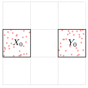
(a) Point set pair for $\mathcal{H}$ construction

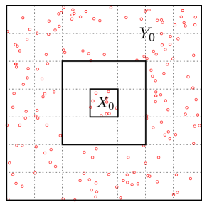
(b) Point set pair for $\mathcal{H}^{2}$ construction

Figure 1: Examples of point set pairs $X_{0}\times Y_{0}$ in the approximated low-rank blocks with a strong admissibility condition.

Using an algebraic approach, interpolative decomposition (ID) [9, 6], QR variants, adaptive cross approximation (ACA) [3, 2] and randomized rank-revealing algorithms [15] are widely used in hierarchical matrix construction. Most of these algebraic methods take at least $O(r|X_{0}||Y_{0}|)$ with the obtained rank $r$. The only exception is ACA with complexity $O(r^{2}(|X_{0}|+|Y_{0}|))$ but its validity is based on the smoothness of the kernel function and certain admissibility conditions.

Using an analytic approach, low-rank approximations of $K(X_{0},Y_{0})$ can be obtained by a degenerate function approximation of $K(x,y)$, i.e., a finite expansion with separated variables like the summation term in Equation 1. Such an approach only requires $O(r(|X_{0}|+|Y_{0}|))$ computation. Typical strategies include Taylor expansion, as in panel clustering [14], and multipole expansion, as in FMM [8]. However, the obtained rank $r$ can be much larger than those by algebraic methods and explicit expansions are only available for a few standard kernels.

There are also several hybrid algebraic-analytic compression algorithms such as those used in kernel-independent FMM (KIFMM) [19], recursive skeletonization [18, 16] and SMASH [4]. These algorithms share the same strategy of taking advantage of having an analytic kernel but without having any explicit expansion of $K(x,y)$. This strategy is combined with purely algebraic methods to help reduce the computational cost. However, the validity of both KIFMM and recursive skeletonization is only proved for kernels from potential theory, and SMASH needs a heuristic selection of the rank for certain kernel matrix blocks and the basis functions for degenerate function approximation of $K(x,y)$.

Following the same strategy as the above hybrid algorithms, we introduce a new algorithm for the low-rank approximation of $K(X_{0},Y_{0})$ for general kernel functions that implicitly uses the putative degenerate function approximation. The method also uses the ID by strong rank-revealing QR (sRRQR) [9] but reduces the construction cost from $O(r|X_{0}||Y_{0}|)$, for ID using sRRQR alone, to $O(r|X_{0}|)$. The proposed algorithm only requires kernel evaluations and can automatically determine the rank for a given error threshold.

2 Background

In this paper, we focus on the approximation of blocks in ID-based $\mathcal{H}^{2}$ construction but the same ideas can be easily adapted to $\mathcal{H}$ construction.

Hierarchical matrix construction is based on a hierarchical partitioning of a box domain in $\mathbb{R}^{d}$ where the box encloses all the prescribed points. Defining this box as the root level, finer partitions at subsequent levels are obtained by recursively subdividing every box at the previous level uniformly into $2^{d}$ smaller boxes until the number of points in each finest box is less than a prescribed constant. In ID-based $\mathcal{H}^{2}$ construction, each non-empty box $\mathcal{B}_{i}$ at any non-root level is associated with an ID approximation of a sub-block $K(X_{i},Y_{i})$ where $X_{i}$ is some subset of the points lying in $\mathcal{B}_{i}$ and $Y_{i}$ is some subset of the points lying in the union of boxes at the same level that are admissible with $\mathcal{B}_{i}$. Readers can refer to [16, 4] for more details.

Since $K(x,y)$ is translation-invariant and boxes at the same level are of the same size, the approximations of $K(X_{i},Y_{i})$ associated with these different boxes $\mathcal{B}_{i}$ at the same level can all be unified into the following single problem.

Problem 1

Find an ID approximation of $K(X_{0},Y_{0})$ with point sets $X_{0}\subset\mathcal{X}$ and $Y_{0}\subset\mathcal{Y}$ where $\mathcal{X}$ is a fixed box and $\mathcal{Y}$ is the union of all the boxes that have the same size as $\mathcal{X}$ and are admissible with $\mathcal{X}$. The domain $\mathcal{Y}$ is referred to as the far field of $\mathcal{X}$ by the prescribed admissibility condition. In practice, we only consider $\mathcal{Y}$ as a bounded sub-domain of the far field. Examples of $\mathcal{X}\times\mathcal{Y}$ are illustrated in Figure 2.

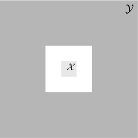
(a) Strong admissibility condition

(b) Weak admissibility condition

Figure 2: Examples of the domain pair $\mathcal{X}\times\mathcal{Y}$ in 2D.

A simple one-dimensional example in Figure 3 illustrates the associated low-rank approximations needed in one level of ID-based $\mathcal{H}^{2}$ construction and the way to convert these approximation problems into 1 using translations.

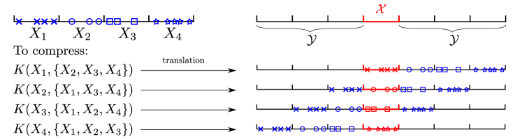
Figure 3: Example of low-rank approximations in one partition level of the ID-based $\mathcal{H}^{2}$ construction. The weak admissibility condition is applied but the strong admissibility scenario can be handled similarly. $X_{1}$, $X_{2}$, $X_{3}$ and $X_{4}$ are point sets in the subintervals at the finer level of a two-level hierarchical partitioning of the whole interval. For each point set $X_{i}$, the ID approximation of $K(X_{i},\cup_{j=1}^{4}X_{j}\backslash X_{i})$ is needed. With a proper selection of domain pair $\mathcal{X}\times\mathcal{Y}$ as shown in the figure, every approximation problem can be converted to 1 using translation.

The interpolative decomposition [9, 6] is extensively used in this paper. Since somewhat different definitions exist in the literature, we give our definition as follows. Given a matrix $A\in\mathbb{R}^{n\times m}$, a rank-$k$ ID approximation of $A$ is $UA_{J}$ where $A_{J}\in\mathbb{R}^{k\times m}$ is a row subset of $A$ and entries of $U\in\mathbb{R}^{n\times k}$ are bounded. ID here only refers to a form of decomposition and there exist many ways of computing it with different accuracies. In particular, minimizing the approximation error in the Frobenius norm, the optimal $U$ for an ID with a fixed $A_{J}$ can be calculated as $U=AA_{J}^{{\dagger}}$ by projecting each row of $A$ onto the row space of $A_{J}$.

Define $UA_{J}$ as an ID with error threshold $\varepsilon$ if the norm of each row of the error matrix $A-UA_{J}$ is bounded by $\varepsilon$. The ID can be calculated algebraically by applying strong rank-revealing QR (sRRQR) [9] to $A^{T}$. Truncating the obtained sRRQR decomposition of $A^{T}$ with absolute error threshold $\varepsilon$ as

$$A^{T}P=\left(A_{1}^{T}\ A_{2}^{T}\right)=\left(Q_{1}\ Q_{2}\right)\left(\begin{smallmatrix}R_{11}&R_{12}\\ &R_{22}\end{smallmatrix}\right)\approx Q_{1}\left(R_{11}\ R_{12}\right)=A_{1}^{T}\left(I\ \ R_{11}^{-1}R_{12}\right),$$

the ID with error threshold $\varepsilon$ is then $A\approx P\left(\begin{smallmatrix}I\\ (R_{11}^{-1}R_{12})^{T}\end{smallmatrix}\right)A_{1}$ where $P$ is a permutation matrix. sRRQR can guarantee that the entries of $R_{11}^{-1}R_{12}$ are bounded by a pre-specified parameter $C\geqslant 1$. The complexity of this algorithm is typically $O(rnm)$ but, in rare cases, it may become $O(n^{2}m)$.

2.1 Accelerated compression via a proxy surface

For 1 with kernels from potential theory, Martinsson and Rokhlin [18] accelerate the ID approximation by using the concept of a proxy surface. Specifically, take the Laplace kernel $K(x,y)$ in 2D as an example and consider the domain pair $\mathcal{X}\times\mathcal{Y}$ and the interior boundary of $\mathcal{Y}$, denoted as $\Gamma$, shown in Figure 4.

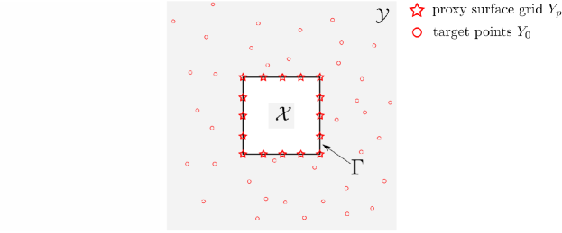
Figure 4: Accelerated compression via a proxy surface. The matrix to be directly compressed changes from the target matrix $K(X_{0},Y_{0})$ to matrix $K(X_{0},Y_{p})$ with a constant column size $|Y_{p}|$, regardless of how many points $Y_{0}$ there are in $\mathcal{Y}$.

By virtue of Green’s Theorem, the potential field in $\mathcal{X}$ generated by charges at $Y_{0}\subset\mathcal{Y}$ can be equivalently generated by charges on $\Gamma$ which encloses $\mathcal{X}$. The surface $\Gamma$ is referred to as a proxy surface in [16]. Discretizing $\Gamma$ with a grid point set $Y_{p}$, it can be proved [18] that

$$K(x,Y_{0})\approx K(x,Y_{p})W,\quad\forall x\in\mathcal{X},$$ (2)

where $W$ is a discrete approximation of the operator that maps charges at $Y_{0}$ to an equivalent charge distribution on $\Gamma$ and $\|W\|_{2}$ is bounded as a consequence of Green’s Theorem. Thus, the target matrix $K(X_{0},Y_{0})$ can be approximated as $K(X_{0},Y_{p})W$ and compressing $K(X_{0},Y_{0})$ directly by ID using sRRQR is accelerated as follows.

First find an ID approximation of $K(X_{0},Y_{p})$ as $UK(X_{\text{rep}},Y_{p})$ by sRRQR where $X_{\text{rep}}\subset X_{0}$ denotes the “representative” point subset associated with the selected row subset and $U$ is the matrix obtained from the ID. The approximation of $K(X_{0},Y_{0})$ is then defined as $UK(X_{\text{rep}},Y_{0})$. By Equation 2, the approximation error can be bounded as

$$\|K(X_{0},Y_{0})-UK(X_{\text{rep}},Y_{0})\|_{F} \approx\|\left(K(X_{0},Y_{p})-UK(X_{\text{rep}},Y_{p})\right)W\|_{F}$$

$$\leqslant\|K(X_{0},Y_{p})-UK(X_{\text{rep}},Y_{p})\|_{F}\|W\|_{2},$$

and thus the accelerated approximation can control the error.

The number of points to discretize $\Gamma$ (i.e., $|Y_{p}|$) is heuristically decided and only depends on the desired precision and the geometry of $\mathcal{X}$ and $\Gamma$. Thus, the algorithm complexity, i.e., $O(|X_{\text{rep}}||X_{0}||Y_{p}|)$, is independent of $|Y_{0}|$. Practically, this method only applies to $\mathcal{X}\times\mathcal{Y}$ with strong admissibility conditions since when $\mathcal{X}$ and $\Gamma$ are close, very large $|Y_{p}|$ is needed due to the singularity of $K(x,y)$.

The key for this method is the relation Equation 2 and the well-conditioning of $W$ that are both analytically derived from Green’s Theorem. Thus, the method is only rigorously valid for kernels from potential theory and its generalization to certain problems may deteriorate or require further modifications as discussed in [18]. The above method will be referred to as proxy-surface method.

In this paper, we develop an analogous compression algorithm for general kernels that only depends on the existence of an accurate degenerate function approximation of $K(x,y)$. In the new algorithm, the above heuristically selected point set $Y_{p}$ that discretizes $\Gamma$ will instead be selected from the whole domain $\mathcal{Y}$.

2.2 Notation

Let $\mathcal{X}\times\mathcal{Y}$ be a compact domain pair in $\mathbb{R}^{d}$ as described in 1 with a certain admissibility condition and $K(x,y)$ be a translation-invariant kernel function in $\mathbb{R}^{d}$ and smooth in $\mathcal{X}\times\mathcal{Y}$. Denote the Karhunen-Loève (KL) decomposition of $K(x,y)$ over $\mathcal{X}\times\mathcal{Y}$ as

$$K(x,y)=\sum_{i=1}^{\infty}\sigma_{i}\psi_{i}(x)\phi_{i}(y),\quad x\in\mathcal{X},y\in\mathcal{Y},$$ (3)

where $\{\psi_{i}(x)\}$ and $\{\phi_{i}(y)\}$ are sets of orthonormal functions in $\mathcal{X}$ and $\mathcal{Y}$ respectively and $\{\sigma_{i}\}$ is a sequence of decaying non-negative real numbers. As the series converges uniformly, there exists a minimal index $r$ such that

$$\left|K(x,y)-\sum_{i=1}^{r}\sigma_{i}\psi_{i}(x)\phi_{i}(y)\right|\leqslant\varepsilon_{\text{machine}},\quad\forall x\in\mathcal{X},\ \forall y\in\mathcal{Y}.$$ (4)

For any finite point sets $X_{0}\subset\mathcal{X}$ and $Y_{0}\subset\mathcal{Y}$, $K(X_{0},Y_{0})$ can then be written as

$$K(X_{0},Y_{0})=\Psi(X_{0})^{T}\left(\begin{smallmatrix}\sigma_{1}&&&\\ &\sigma_{2}&&\\ &&\ldots&&\\ &&&\sigma_{r}\end{smallmatrix}\right)\Phi(Y_{0})+E,$$ (5)

where the entries of $E$ are bounded by $\varepsilon_{\text{machine}}$, $\Psi(x)=(\psi_{i}(x))_{i=1}^{r}$ and $\Phi(y)=(\phi_{i}(y))_{i=1}^{r}$ are column vector functions and $\Psi(X_{0})$ with $X_{0}=\{x_{i}\}_{i=1}^{n}$ is defined as

$$\Psi(X_{0})=\left(\Psi(x_{1})\ \Psi(x_{2})\ \ldots\ \Psi(x_{n})\right)\in\mathbb{R}^{r\times n}.$$ (6)

We define $\Phi(Y_{0})$ in the same manner. In this paper, the evaluation of any function over a point set is defined in the same way as above. In particular, for a scalar function like $\psi_{i}(x)$, $\psi_{i}(X_{0})$ denotes a row vector of length $|X_{0}|$. Based on Equation 5, the numerical rank of $K(X_{0},Y_{0})$ for any point set pair $X_{0}\times Y_{0}$ is $r$ or less.

For the following discussion, we consider the simplified case where $K(x,y)$ over $\mathcal{X}\times\mathcal{Y}$ is a degenerate function, i.e., its KL expansion only has a finite number of terms as

$$K(x,y)=\sum_{i=1}^{r_{\text{KL}}}\sigma_{i}\psi_{i}(x)\phi_{i}(y),\quad x\in\mathcal{X},y\in\mathcal{Y},r_{\text{KL}}<\infty.$$ (7)

A non-degenerate kernel over $\mathcal{X}\times\mathcal{Y}$ can be approximated by the first $r$ terms of its KL expansion with $r$ satisfying Equation 4. The effect of the error $\sum_{i=r+1}^{\infty}\sigma_{i}\psi_{i}(x)\phi_{i}(y)$, which is bounded by $\varepsilon_{\text{machine}}$, on the following proposed algorithm can be analyzed through a stability analysis which we leave as future work.

3 Algorithm description

Denoting $X_{0}\subset\mathcal{X}$ and $Y_{0}\subset\mathcal{Y}$ as given point sets, our goal is to find an approximation of the target matrix $K(X_{0},Y_{0})$ in the form of an ID that is more efficient than using sRRQR.

The key for ID approximation is to find a row subset of $K(X_{0},Y_{0})$, i.e., a subset of $\{K(x_{i},Y_{0})\}_{x_{i}\in X_{0}}$, whose span is close to each row vector $K(x_{i},Y_{0})$. Regarding $K(x_{i},Y_{0})$ as function values of $K(x_{i},y)$ at $Y_{0}$, it is then sufficient to consider the above problem in terms of the functions $\{K(x_{i},y)\}_{x_{i}\in X_{0}}$ in the domain $\mathcal{Y}$. Specifically, we seek a function subset of $\{K(x_{i},y)\}_{x_{i}\in X_{0}}$ whose span is close to each function $K(x_{i},y)$ in $\mathcal{Y}$.

The above “ID approximation” of functions $\{K(x_{i},y)\}_{x_{i}\in X_{0}}$ in $\mathcal{Y}$ is a continuous problem. Heuristically, we can use a uniform grid point set $Y_{p}$ in $\mathcal{Y}$ to discretize the function $K(x_{i},y)$ as $K(x_{i},Y_{p})$, transforming the problem into finding an ID approximation of $K(X_{0},Y_{p})$. In general, $Y_{p}$ should be dense enough to accurately characterize $K(x_{i},y)$ in $\mathcal{Y}$ but this is inefficient in general. However, by the finite KL expansion in Equation 7, $K(x_{i},y)$ for any $x_{i}\in X_{0}$ is in the $r_{\text{KL}}$-dimensional function space spanned by $\phi_{1}(y)$, $\phi_{2}(y)$, …, $\phi_{r_{\text{KL}}}(y)$. Since $\{\phi_{i}(y)\}_{i=1}^{r_{\text{KL}}}$ are orthonormal in $\mathcal{Y}$, to uniquely determine $K(x_{i},y)$, the selected finite point set $Y_{p}\subset\mathcal{Y}$ only needs to satisfy

$$|Y_{p}|\geqslant r_{\text{KL}},\ \text{col}(\Phi(Y_{p}))=\mathbb{R}^{r_{\text{KL}}}.$$ (8)

Importantly, these are points selected from the entire domain $\mathcal{Y}$, not just from $Y_{0}$ or the boundary $\Gamma$ of $\mathcal{Y}$ and we refer these points as proxy points. We expect an effective $Y_{p}$ to satisfy $|Y_{p}|\sim O(r_{\text{KL}})$ and $|Y_{p}|\ll|Y_{0}|$ in real situations.

With a proxy point set $Y_{p}$ that satisfies Equation 8, the following algorithm is proposed to find an ID approximation of $K(X_{0},Y_{0})$ through an “ID approximation” of $\{K(x_{i},y)\}_{x_{i}\in X_{0}}$ in $\mathcal{Y}$.

Step 1

Find an ID approximation of $K(X_{0},Y_{p})$ with error threshold $\varepsilon$ by sRRQR as

$$K(X_{0},Y_{p})\approx W_{\text{rep}}K(X_{\text{rep}},Y_{p}),$$ (9)

where $X_{\text{rep}}\subset X_{0}$ denotes the point set associated with the selected row subset and $W_{\text{rep}}=K(X_{0},Y_{p})K(X_{\text{rep}},Y_{p})^{\dagger}$ is the obtained matrix from the ID.

Step 2

For each $x_{i}\in X_{0}$, denote the $i$th row of $W_{\text{rep}}$ as $w_{i}$ and approximate the function $K(x_{i},y)$ as

$$K(x_{i},y)\approx w_{i}^{T}K(X_{\text{rep}},y),\quad y\in\mathcal{Y}.$$ (10)

It is expected that each $K(x_{i},y)$ is close to the span of $\{K(x_{j},y)\}_{x_{j}\in X_{\text{rep}}}$ and the associated approximation above has small error. Evaluating the functions in Equation 10 at $Y_{0}$, row vector $K(x_{i},Y_{0})$ can be approximated by $w_{i}^{T}K(X_{\text{rep}},Y_{0})$ and a rank-$|X_{\text{rep}}|$ ID approximation is then defined as

$$K(X_{0},Y_{0})\approx W_{\text{rep}}K(X_{\text{rep}},Y_{0}).$$ (11)

Both $W_{\text{rep}}$ and $X_{\text{rep}}$ are calculated in Step 1 and only require $O(|X_{\text{rep}}||X_{0}||Y_{p}|)$ computation which is independent of $|Y_{0}|$.

To summarize, the proposed algorithm calculates $\{w_{i}\}$ and $X_{\text{rep}}$ to minimize the function approximation error $K(x_{i},y)-w_{i}^{T}K(X_{\text{rep}},y)$ at $Y_{p}$ to help make the error small over the whole domain $\mathcal{Y}$. Thus, for any $Y_{0}\subset\mathcal{Y}$, the proposed approximation Equation 11 has its entry-wise error bounded by $\max_{x_{i}\in X_{0}}\|K(x_{i},y)-w_{i}^{T}K(X_{\text{rep}},y)\|_{\infty}$. It is worth noting that the rank $|X_{\text{rep}}|$ is fixed for any $Y_{0}\subset\mathcal{Y}$ and is only related to $X_{0}$ and the error threshold $\varepsilon$. A better ID approximation with the selected $X_{\text{rep}}$ can be obtained by replacing $W_{\text{rep}}$ with $K(X_{0},Y_{0})K(X_{\text{rep}},Y_{0})^{{\dagger}}$ but this requires a computational cost linear in $|Y_{0}|$. Also, $K(X_{\text{rep}},Y_{0})$ does not need to be explicitly formulated in ID-based $\mathcal{H}^{2}$ construction which avoids $|Y_{0}|$-dependent calculations.

4 Algorithm analysis

For any $x\in\mathcal{X}$, define $g_{x}(y)=K(x,y)$ as a function of $y$ in $\mathcal{Y}$. By the finite KL expansion, $g_{x}(y)$ can be represented as

$$g_{x}(y)=u_{x}^{T}\Phi(y),\quad u_{x}=(\sigma_{i}\psi_{i}(x))_{i=1}^{r_{\text{KL}}},\quad\Phi(y)=(\phi_{i}(y))_{i=1}^{r_{\text{KL}}}.$$ (12)

With a proxy point set $Y_{p}$ that satisfies Equation 8, substitute $Y_{p}$ for $y$ in Equation 12 and solve for $u_{x}$ as $u_{x}^{T}=g_{x}(Y_{p})\Phi(Y_{p})^{{\dagger}}$ where $g_{x}(Y_{p})$ is a row vector defined in the obvious way. Thus, $g_{x}(y)$ can be represented in terms of $g_{x}(Y_{p})$ as

$$g_{x}(y)=g_{x}(Y_{p})\Phi(Y_{p})^{{\dagger}}\Phi(y),\quad\forall y\in\mathcal{Y}.$$ (13)

We can then estimate the error of both the function approximation Equation 10 and the proposed ID approximation Equation 11. Denote the error of Equation 10 for each $x_{i}\in X_{0}$ as

$$e_{i}(y)=K(x_{i},y)-w_{i}^{T}K(X_{\text{rep}},y),\quad y\in\mathcal{Y}.$$ (14)

The error vector of the $i$th row approximation in Equation 9 and Equation 11 can be exactly represented as $e_{i}(Y_{p})$ and $e_{i}(Y_{0})$, respectively. Since the error threshold for the ID approximation of $K(X_{0},Y_{p})$ is $\varepsilon$, each error vector $e_{i}(Y_{p})$ satisfies $\|e_{i}(Y_{p})\|_{2}<\varepsilon$.

Note that $e_{i}(y)$ is a linear combination of $g_{x_{i}}(y)$ and $\{g_{x_{j}}(y)\}_{x_{j}\in X_{\text{rep}}}$ and Equation 13 holds for $g_{x}(y)$ with any $x\in\mathcal{X}$. Thus, $e_{i}(y)$ has the similar representation

$$e_{i}(y)=e_{i}(Y_{p})\Phi(Y_{p})^{{\dagger}}\Phi(y),$$ (15)

and $e_{i}(y)$ and $e_{i}(Y_{0})$ can be bounded by the error at $Y_{p}$ as

$$|e_{i}(y)| \leqslant\|e_{i}(Y_{p})\|_{2}\|\Phi(Y_{p})^{{\dagger}}\Phi(y)\|_{2}\leqslant\varepsilon\|\Phi(Y_{p})^{{\dagger}}\Phi(y)\|_{2},$$ (16)

$$\|e_{i}(Y_{0})\|_{2} \leqslant\|e_{i}(Y_{p})\|_{2}\|\Phi(Y_{p})^{{\dagger}}\Phi(Y_{0})\|_{2}\leqslant\varepsilon\|\Phi(Y_{p})^{{\dagger}}\Phi(Y_{0})\|_{2}.$$ (17)

If the choice of $Y_{p}$ can guarantee $\|\Phi(Y_{p})^{{\dagger}}\Phi(Y_{0})\|_{2}$ to be small, the proposed approximation can then be good and its error can be controlled by $\varepsilon$.

5 Selection of the proxy point set

In the proposed algorithm above, the choice of $Y_{p}$ is flexible but critical. The only requirement for $Y_{p}$ is the condition Equation 8 and we desire that $\|\Phi(Y_{p})^{\dagger}\Phi(Y_{0})\|_{2}$ is small.

By the continuity of functions $\{\phi_{i}(y)\}_{i=1}^{r_{\text{KL}}}$ in the compact domain $\mathcal{Y}$, $\Phi(y)$ is bounded and thus $\|\Phi(Y_{p})^{\dagger}\Phi(Y_{0})\|_{2}$ is also bounded for any $Y_{p}$ satisfying Equation 8. The number of points in $Y_{p}$ also matters since adding more points to $Y_{p}$ can reduce $\|\Phi(Y_{p})^{\dagger}\Phi(Y_{0})\|_{2}$ monotonically but larger $|Y_{p}|$ leads to more computation for the ID approximation of $K(X_{0},Y_{p})$. Thus, a constraint like $|Y_{p}|=O(r_{\text{KL}})$ is necessary to balance the trade-off.

However, $\psi_{i}(x)$, $\phi_{i}(y)$ and $r_{\text{KL}}$ are usually not available for a general kernel function over a domain pair. We only assume that $K(x,y)$ over $\mathcal{X}\times\mathcal{Y}$ has a finite KL expansion. For a non-degenerate kernel, this assumption means that there is a truncation of the KL expansion with error satisfying Equation 4. In both degenerate and non-degenerate cases, the number of expansion terms (i.e., $r_{\text{KL}}$) only depends on the kernel and the domain pair $\mathcal{X}\times\mathcal{Y}$. Thus, condition Equation 8 cannot be directly checked for any point set $Y_{p}$. The only property we can use is based on Equation 5, that $r_{\text{KL}}$ is an upper bound of the numerical rank of $K(X_{0},Y_{0})$ with any point set pair $X_{0}\times Y_{0}\subset\mathcal{X}\times\mathcal{Y}$.

Based on the analysis above, the first method to select $Y_{p}$ is proposed as follows.

Random Selection

Choose $Y_{p}$ as a set of points that are randomly and uniformly distributed in $\mathcal{Y}$ so that condition Equation 8 is likely to hold. The size of $Y_{p}$ can be heuristically decided as the maximum numerical rank of $K(X_{0},Y_{0})$, with some tentative $X_{0}\times Y_{0}\subset\mathcal{X}\times\mathcal{Y}$, plus a small redundancy constant.

This selection turns out to be effective in many numerical tests. However, it does not guarantee the scaling factor $\|\Phi(Y_{p})^{\dagger}\Phi(Y_{0})\|_{2}$ to be small and thus the proposed algorithm may have much larger error than that of algebraic methods with the same approximation rank in some cases.

A better selection of $Y_{p}$ should also try to minimize $\|\Phi(Y_{p})^{{\dagger}}\Phi(Y_{0})\|_{2}$. Since the point distribution $Y_{0}$ is problem-dependent and $\|\Phi(Y_{p})^{{\dagger}}\Phi(Y_{0})\|_{2}$ can be bounded as

$$\|\Phi(Y_{p})^{{\dagger}}\Phi(Y_{0})\|_{2}\leqslant\|\Phi(Y_{p})^{{\dagger}}\Phi(Y_{0})\|_{F}\leqslant\sqrt{|Y_{0}|}\max_{y\in\mathcal{Y}}\|\Phi(Y_{p})^{{\dagger}}\Phi(y)\|_{2},$$

we only need to consider the choice of $Y_{p}$ to minimize $\|\Phi(Y_{p})^{{\dagger}}\Phi(y)\|_{2}$.

Denote $S_{Y_{p}}(y)=\Phi(Y_{p})^{{\dagger}}\Phi(y)$ as the solution of the least squares problem

$$\Phi(Y_{p})S_{Y_{p}}(y)=\Phi(y).$$ (18)

Since $\{\psi_{i}(x)\}_{i=1}^{r_{KL}}$ are orthonormal in $\mathcal{X}$ and $u_{x}=(\sigma_{i}\psi_{i}(x))_{i=1}^{r_{\text{KL}}}$, we can select a point set $X_{p}\subset\mathcal{X}$ such that

$$|X_{p}|\geqslant{r_{\text{KL}}},\ \text{span}\{u_{x},x\in X_{p}\}=\mathbb{R}^{r_{\text{KL}}}=\text{col}(\Psi(X_{p})).$$ (19)

Based on $K(x,y)=u_{x}^{T}\Phi(y)$ and Equation 18, it can be verified that $S_{Y_{p}}(y)$ is also the solution of the least squares problem $K(X_{p},Y_{p})S_{Y_{p}}(y)=K(X_{p},y)$. As a result, $S_{Y_{p}}(y)$ can be represented differently as

$$S_{Y_{p}}(y)=K(X_{p},Y_{p})^{{\dagger}}K(X_{p},y)=\Phi(Y_{p})\Phi(y),$$ (20)

with any $X_{p}$ satisfying Equation 19. By this new representation, the second method for the selection of $Y_{p}$ is described as follows.

ID Selection

Select two point sets $X_{d}\subset\mathcal{X}$ and $Y_{d}\subset\mathcal{Y}$ that are dense enough so that Equation 19 and Equation 8 are likely to hold. Find an ID approximation of $K(X_{d},Y_{d})^{T}$ by sRRQR as

$$K(X_{d},Y_{d})\approx K(X_{d},Y_{\text{rep}})U=K(X_{d},Y_{\text{rep}})\Big{(}K(X_{d},Y_{\text{rep}})^{\dagger}K(X_{d},Y_{d})\Big{)}$$

where the error threshold is set as $\sqrt{|X_{d}|}\varepsilon_{\text{machine}}$ to estimate the numerical rank of $K(X_{d},Y_{d})$ and it is expected that the rank $|Y_{\text{rep}}|\approx r_{\text{KL}}$. Then, the point subset $Y_{\text{rep}}$ selected by the ID approximation can be used as the proxy point set $Y_{p}$. The detailed algorithm is shown in Algorithm 1.

Algorithm 1 Selection of the proxy point set $Y_{p}$

0:  kernel function $K(x,y)$, domain pair $\mathcal{X}\times\mathcal{Y}$.

0:  proxy point set $Y_{p}$.

1:  Select uniform grid point sets $X_{d}$ and $Y_{d}$ in $\mathcal{X}$ and $\mathcal{Y}$ respectively. $Y_{d}$ is referred to as a candidate set.

2:  Find an ID approximation of $K(X_{d},Y_{d})^{T}$ with error threshold $\sqrt{|X_{d}|}\varepsilon_{\text{machine}}$ by sRRQR. Define $Y_{p}$ as the point subset of $Y_{d}$ associated with the selected rows.

3:  If $|Y_{p}|=\min(|X_{d}|,|Y_{d}|)$, select denser grids for $X_{d}$, $Y_{d}$ and repeat the whole process. Otherwise, $Y_{p}$ is the selected proxy point set.

By the sRRQR used in the ID approximation, the entries of $U$ are bounded by a pre-specified parameter $C\geqslant 1$. Equivalently, for any $y\in Y_{d}$, $K(X_{d},Y_{\text{rep}})^{\dagger}K(X_{d},y)$, as a column of $U$, has all its entries bounded by $C$. Since $K(x,y)$ is smooth and $Y_{d}$ is dense in $\mathcal{Y}$, entries of $K(X_{d},Y_{\text{rep}})^{{\dagger}}K(X_{d},y)$ can also be roughly bounded by $C$ for any $y\in\mathcal{Y}$. Thus, it holds that $\|S_{Y_{p}}(y)\|_{2}\lesssim\sqrt{|Y_{p}|}C$ for any $y\in\mathcal{Y}$. By the inequalities Equation 16 and Equation 17, we can obtain upper bounds for $|e_{i}(y)|$ and $\|e_{i}(Y_{0})\|_{2}$ as

$$|e_{i}(y)| \lesssim\sqrt{|Y_{p}|}C\varepsilon,\qquad\forall y\in\mathcal{Y},$$ (21)

$$\|e_{i}(Y_{0})\|_{2} \lesssim\sqrt{|Y_{0}||Y_{p}|}C\varepsilon.$$ (22)

Since both $|Y_{p}|\sim O(r_{\text{KL}})$ and $C$ are small, we expect the average entry-wise error $\|e_{i}(Y_{0})\|_{2}/\sqrt{|Y_{0}|}$ to be $O(\varepsilon)$.

Algorithm 1 has complexity $O(|Y_{p}||X_{d}||Y_{d}|)$ where $|Y_{p}|$, as an estimate of $r_{\text{KL}}$, only depends on the kernel and the domain pair $\mathcal{X}\times\mathcal{Y}$. Although requiring significant calculation, Algorithm 1 is only a pre-processing step and only needs to be applied once for one domain pair $\mathcal{X}\times\mathcal{Y}$. As described in the context of 1, in ID-based $\mathcal{H}^{2}$ construction, all the cluster pairs $\{X_{i}\times Y_{i}\}$ that are associated with sub-domains at the same level can fit to one domain pair $\mathcal{X}\times\mathcal{Y}$ by translations. Thus, for the compression of all these blocks $K(X_{i},Y_{i})$, the proxy point set $Y_{p}$ can be reused.

6 Comparison with existing methods

In this section, we qualitatively compare our proposed algorithm with existing methods for the low-rank approximation of $K(X_{0},Y_{0})$ with $X_{0}\times Y_{0}$ in some domain pair $\mathcal{X}\times\mathcal{Y}$.

In ID using sRRQR, each $K(x_{i},y)$ is well approximated by $w_{i}^{T}K(X_{\text{rep}},y)$ for $y\in Y_{0}$. The proposed algorithm, on the other hand, approximates each $K(x_{i},y)$ by $w_{i}^{T}K(X_{\text{rep}},y)$ for $y$ in the domain $\mathcal{Y}$ that contains $Y_{0}$. Thus, the proposed algorithm generally selects a larger row subset and the obtained $w_{i}$ does not necessarily minimize $\|K(x_{i},Y_{0})-w_{i}^{T}K(X_{\text{rep}},Y_{0})\|_{2}$.

It is also worth noting that the proxy-surface method described in Section 2.1 is equivalent to the proposed algorithm when $Y_{p}$ is chosen to discretize the interior boundary $\Gamma$ of $\mathcal{Y}$. We refer to this selection of $Y_{p}$ as Surface Selection. Just like Random Selection, the number of points in $Y_{p}$ needs to be manually decided in this selection scheme. For kernels from potential theory, it has been shown analytically in Section 2.1 that Surface Selection of $Y_{p}$ is sufficient for the proposed algorithm to be effective. However, for general kernels, this selection scheme usually leads to much larger error in comparison with Random and ID Selection schemes in our numerical experiments.

6.1 Comparison with algebraic and analytic methods

In general, an analytic method seeks a degenerate approximation of $K(x,y)$ over $\mathcal{X}\times\mathcal{Y}$ as

$$K(x,y)\approx\sum_{i=1}^{r}f_{i}(x)h_{i}(y),\quad x\in\mathcal{X},y\in\mathcal{Y},$$ (23)

with some analytically calculated functions $\{f_{i}(x)\}$ and $\{h_{i}(y)\}$.

An algebraic method, on the other hand, seeks a degenerate approximation of $K(x,y)$ over $X_{0}\times Y_{0}$ instead. Denoting an obtained low-rank approximation as $K(X_{0},Y_{0})\approx F^{T}H$ with $F\in\mathbb{R}^{r\times|X_{0}|}$ and $H\in\mathbb{R}^{r\times|Y_{0}|}$, the degenerate approximation can be defined as Equation 23 with $\mathcal{X}\times\mathcal{Y}$ replaced by $X_{0}\times Y_{0}$ and

$$f_{i}(x)=\sum_{x_{j}\in X_{0}}F_{ij}\delta_{x_{j}}(x),\quad h_{i}(y)=\sum_{y_{j}\in Y_{0}}H_{ij}\delta_{y_{j}}(y),$$ (24)

where $\delta_{v}(z)=\left\{\begin{array}[]{ll}1,&\ z=v\\ 0,&\ z\neq v\end{array}\right.$ is the delta function.

Similarly, the proposed algorithm can be regarded as seeking a degenerate approximation of $K(x,y)$ over $X_{0}\times\mathcal{Y}$. The degenerate approximation can still be defined as Equation 23 with $\mathcal{X}\times\mathcal{Y}$ replaced by $X_{0}\times\mathcal{Y}$, the summation over $x_{i}\in X_{\text{rep}}$ and

$$f_{i}(x)=\sum_{x_{j}\in X_{0}}(W_{\text{rep}})_{ji}\delta_{x_{j}}(x),\quad h_{i}(y)=K(x_{i},y).$$ (25)

Theoretically, the optimal degenerate approximation (i.e., the expansion with least terms to meet the same accuracy criteria) of $K(x,y)$ in a smaller domain pair should have fewer expansion terms. As $X_{0}\times Y_{0}\subset X_{0}\times\mathcal{Y}\subset\mathcal{X}\times\mathcal{Y}$, algebraic methods can obtain the smallest optimal rank while analytic methods deliver the largest optimal rank among the three classes of methods. Our proposed algorithm lies between analytic and algebraic methods and can be regarded as balancing between computational cost, where analytic methods are better, and optimal rank estimation, where algebraic methods are better.

6.2 Comparison with KIFMM

Here, we focus on the source to multipole (S2M) translation phase in KIFMM. Similar comparisons with the other phases can be easily established.

An illustration of the S2M phase in KIFMM is shown in Figure 5. Taking the Laplace kernel $K(x,y)$ in 2D as an example, the potential $q(y)$ at $y\in\mathcal{Y}$ generated by a source point set $X_{0}$ with charges $\{f_{i}\}$ is calculated as

$$q(y)=\sum_{x_{i}\in X_{0}}K(x_{i},y)f_{i}=K(X_{0},y)^{T}F,$$ (26)

where $K(X_{0},y)=(K(x_{i},y))_{x_{i}\in X_{0}}$ and $F=(f_{i})_{x_{i}\in X_{0}}$ are column vectors.

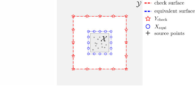
Figure 5: 2D illustration of the S2M phase in KIFMM. The strong admissibility condition is applied over $\mathcal{X}\times\mathcal{Y}$. The equivalent surface lies between $\mathcal{X}$ and $\mathcal{Y}$ and encloses $\mathcal{X}$, and the check surface lies between $\mathcal{Y}$ and the equivalent surface. The potential at $y\in\mathcal{Y}$ generated by source charges in $\mathcal{X}$ is expected to be also generated by equivalent charges distributed on the equivalent surface. The equivalent charges can be determined by matching their induced potential on the check surface with that induced by the source charges. $X_{\text{equi}}$ and $Y_{\text{check}}$ are the discretization points of the associated surfaces.

KIFMM calculates the equivalent charges $\tilde{F}$ at grid points $X_{\text{equi}}$ on the equivalent surface by matching the potentials at grid points $Y_{\text{check}}$ on a check surface generated by both $F$ and $\tilde{F}$ as

$$K(X_{\text{equi}},Y_{\text{check}})^{T}\tilde{F}=K(X_{0},Y_{\text{check}})^{T}F.$$ (27)

The potential at $y$ is then approximated as

$$q(y) =K(X_{0},y)^{T}F$$

$$\approx K(X_{\text{equi}},y)^{T}\tilde{F}=K(X_{\text{equi}},y)^{T}(K(X_{\text{equi}},Y_{\text{check}})^{T})^{{\dagger}}K(X_{0},Y_{\text{check}})^{T}F.$$

This approximation applies to any charge vector $F$ and source points $X_{0}\subset\mathcal{X}$. Thus, it is equivalent to approximating $K(x,y)$ over $\mathcal{X}\times\mathcal{Y}$ as

$$K(x,y)\approx K(x,Y_{\text{check}})K(X_{\text{equi}},Y_{\text{check}})^{{\dagger}}K(X_{\text{equi}},y).$$ (28)

For the proposed algorithm, combining the equations Equation 13 and Equation 20, it holds that

$$K(x,y)=K(x,Y_{p})K(X_{p},Y_{p})^{{\dagger}}K(X_{p},y).$$ (29)

For non-degenerate kernels, the above equation becomes an approximation that shares exactly the same form as Equation 28.

From the above discussion, the S2M phase in KIFMM and the proposed algorithm are based on a similar degenerate approximation of $K(x,y)$ over $\mathcal{X}\times\mathcal{Y}$. However, in the proposed algorithm, $X_{p}$ and $Y_{p}$ are free to be selected in the whole domain pair $\mathcal{X}\times\mathcal{Y}$ while $X_{\text{equi}}$ and $Y_{\text{check}}$ are restricted to be on the pre-defined equivalent surface and check surface respectively. In addition, the proposed algorithm only implicitly depends on Equation 29 and also takes into account $X_{0}$ to automatically determine the rank $r$ for a given error threshold. For the S2M phase in KIFMM, the rank of the underlying approximation Equation 28 is fixed to be $|X_{\text{equi}}|$ and needs to be manually decided. It should be expected that for general kernels where no Green’s Theorem exists, Equation 28 might not be accurate due to the restriction of the locations of $X_{\text{equi}}$ and $Y_{\text{check}}$, just like the proxy-surface method.

7 Numerical experiments

The basic settings for all the numerical experiments are as follows.

• Two kernels are tested: $K_{1}(x,y)=1/|x-y|$ and $K_{2}(x,y)=\sqrt{1+|x-y|^{2}}$. $K_{1}(x,y)$ is the Laplace kernel in 3D where the proxy-surface method works.

• The tested domains are selected as follows with dimension $d=2,3$.

  • Far-apart domain pair: $\mathcal{X}=[-1,1]^{d},\mathcal{Y}=[-9,9]^{d}\backslash[-3,3]^{d}$,

  • Nearby domain pair: $\mathcal{X}=[-1,1]^{d},\mathcal{Y}=[-9,9]^{d}\backslash[-1.1,1.1]^{d}$.

• Point sets $X_{0}$ and $Y_{0}$ are all uniformly and randomly distributed within $\mathcal{X}$ and $\mathcal{Y}$, respectively, unless otherwise specified.

• The error threshold for the ID approximation of $K(X_{0},Y_{p})$ is set as $10^{-6}\sqrt{|Y_{p}|}$ so that the average entry-wise approximation error of each row satisfies

  $$\|e_{i}(Y_{p})\|_{2}/\sqrt{|Y_{p}|}\leqslant 10^{-6},\quad\forall x_{i}\in X_{0}.$$

• The entry-bound parameter $C$ for sRRQR in both the ID approximation of $K(X_{0},Y_{p})$ and Algorithm 1 is set to 2.

• Denote the proxy point sets obtained by Random, ID and Surface Selection schemes as $Y_{p}^{\text{rand}}$, $Y_{p}^{\text{id}}$ and $Y_{p}^{\text{surf}}$ respectively. Algorithm 1 for the selection of $Y_{p}^{\text{id}}$ has an initial point set pair $X_{d}\times Y_{d}$ of size approximately $1500\times 15000$. Table 1 lists the sizes of the selected $Y_{p}^{\text{id}}$ and the Matlab runtime of Algorithm 1 with different settings. Figure 6 shows the selected $Y_{p}^{\text{id}}$ for the two kernels for the far-apart domain pair in 2D. The number of points in $Y_{p}^{\text{rand}}$ is set to 2000 based on the results of $|Y_{p}^{\text{id}}|$ in Table 1.

  Table 1: Proxy point set size $|Y_{p}^{\text{id}}|$ and runtime of Algorithm 1 with different settings (#/sec.).

  	$K_{1}(x,y)$		$K_{2}(x,y)$
  	2D	3D	2D	3D
  Far-apart domain	174/5.35	636/9.05	126/7.83	821/13.32
  Nearby domain	500/4.98	797/8.93	316/10.90	991/14.16

  

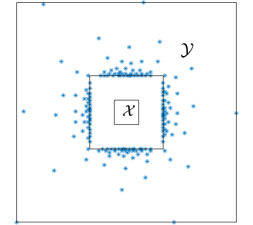
  (a) $K_{1}(x,y)\!=\!1/|x\!-\!y|$ with $|Y_{p}^{\text{id}}|=174$

  

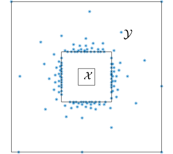
  (b) $K_{2}(x,y)\!=\!\sqrt{1\!+\!|x\!-\!y|^{2}}$ with $|Y_{p}^{\text{id}}|=126$

  Figure 6: Proxy point set $Y_{p}^{\text{id}}$ for two kernels with far-apart domain pair $\mathcal{X}\times\mathcal{Y}$ in 2D.

7.1 Function approximation error $|e_{i}(y)|$

The accuracy of the proposed approximation can be quantified by the function approximation error $e_{i}(y)$ in $\mathcal{Y}$ that is connected to $e_{i}(Y_{p})$ as $e_{i}(y)=e_{i}(Y_{p})S_{Y_{p}}(y)$ from Equation 15. Viewing a general kernel as a degenerate kernel plus a small remainder, the connection Equation 15 only holds approximately. In this subsection, we check the obtained error $|e_{i}(y)|$ of applying the proposed algorithm to the prescribed non-degenerate kernels.

Consider the far-apart domain pair in 2D and $X_{0}\subset\mathcal{X}$ with 1000 points. With the prescribed error threshold and $Y_{p}^{\text{id}}$, the proposed algorithm obtains $X_{\text{rep}}$ with 35 points for $K_{1}(x,y)$ and 33 points for $K_{2}(x,y)$. Similarly, with $Y_{p}^{\text{rand}}$, the obtained $X_{\text{rep}}$ has 28 points for $K_{1}(x,y)$ and 29 points for $K_{2}(x,y)$. To check $e_{i}(y)$, a dense uniform grid in $\mathcal{Y}$ with approximately 40000 points is defined as $Y_{0}$.

By selecting a large point set $X_{p}$ in $\mathcal{X}$ with $|X_{p}|\gg|Y_{p}|$, $S_{Y_{p}}(Y_{0})$ can be explicitly estimated as $K(X_{p},Y_{p})^{{\dagger}}K(X_{p},Y_{0})$ by Equation 20 and the maximum errors of Equation 15 for the two kernels are then found as

$$\max_{x_{i}\in X_{0},y\in Y_{0}}|e_{i}(y)-e_{i}(Y_{p})S_{Y_{p}}(y)|=\left\{\begin{array}[]{ll}4.20\times 10^{-11}&\text{ for }K_{1}(x,y)\text{ with }Y_{p}^{\text{id}}\\ 5.04\times 10^{-10}&\text{ for }K_{1}(x,y)\text{ with }Y_{p}^{\text{rand}}\\ 2.39\times 10^{-10}&\text{ for }K_{2}(x,y)\text{ with }Y_{p}^{\text{id}}\\ 7.30\times 10^{-9}&\text{ for }K_{2}(x,y)\text{ with }Y_{p}^{\text{rand}}\\ \end{array}\right..$$

By these results, the connection Equation 15 indeed holds approximately and thus the proposed algorithm should work with these non-degenerate kernels.

To check the approximation $K(x_{i},y)\approx w_{i}^{T}K(X_{\text{rep}},y)$ for $x_{i}\in X_{0}\backslash X_{\text{rep}}$, Figure 7 shows the following entry-wise error ratios with both $Y_{p}^{\text{id}}$ and $Y_{p}^{\text{rand}}$,

$$\dfrac{\max_{y\in Y_{0}}|e_{i}(y)|}{\|e_{i}(Y_{p})\|_{2}/\sqrt{|Y_{p}|}}\quad\text{and}\quad\dfrac{\|e_{i}(Y_{0})\|_{2}/\sqrt{|Y_{0}|}}{\|e_{i}(Y_{p})\|_{2}/\sqrt{|Y_{p}|}},\quad\text{for any }x_{i}\in X_{0}\backslash X_{\text{rep}}.$$ (30)

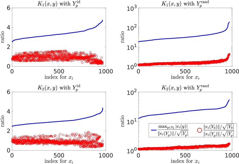
Figure 7: Entry-wise ratios Equation 30 for two kernels with the far-apart domain pair in 2D. Indices for $x_{i}\in X_{0}\backslash X_{\text{rep}}$ are sorted such that the maximum ratios are in ascending order.

By the previous analysis, the entry-wise error ratios in Equation 30 can be bounded as

$$\dfrac{\|e_{i}(Y_{0})\|_{2}/\sqrt{|Y_{0}|}}{\|e_{i}(Y_{p})\|_{2}/\sqrt{|Y_{p}|}}\leqslant\dfrac{\max_{y\in Y_{0}}|e_{i}(y)|}{\|e_{i}(Y_{p})\|_{2}/\sqrt{|Y_{p}|}}\leqslant\sqrt{|Y_{p}|}\max_{y\in Y_{0}}\|S_{Y_{p}}(y)\|_{2}\leqslant|Y_{p}|C$$

where the last inequality only holds for $Y_{p}^{\text{id}}$. From the results in Figure 7, the approximation $K(x_{i},y)\approx w_{i}^{T}K(X_{\text{rep}},y)$ obtained by $Y_{p}^{\text{id}}$ for any $x_{i}\in X_{0}\backslash X_{\text{rep}}$ has its maximum error $e_{i}(y)$ in $\mathcal{Y}$ of the same scale as $e_{i}(Y_{p})/\sqrt{|Y_{p}|}$ which is bounded by $10^{-6}$. Thus, given any $Y_{0}\subset\mathcal{Y}$, the proposed approximation of $K(X_{0},Y_{0})$ should have entry-wise error of the same scale as $10^{-6}$. Also, these results suggest that the above analytic upper bound may not be sharp for $Y_{p}^{\text{id}}$.

From the results for $Y_{p}^{\text{rand}}$, $\|S_{Y_{p}^{\text{rand}}}(y)\|_{2}$ is large for some $y\in\mathcal{Y}$ that leads to very large $e_{i}(y)$. However, the average entry-wise error is still of scale $10^{-6}$ for each $e_{i}(y)$, which indicates that $\|S_{Y_{p}^{\text{rand}}}(y)\|_{2}$ may be small for $y$ in most of the domain $\mathcal{Y}$. Lastly, it is worth noting that ID Selection obtains much better results with much fewer proxy points compared to Random Selection.

7.2 Comparison with algebraic methods

With a fixed cluster set $X_{0}$ and the prescribed error threshold, assume that the proposed algorithm with $Y_{p}^{\text{id}}$ gives a rank-$|X_{\text{rep}}|$ approximation $K(X_{0},Y_{0})\approx W_{\text{rep}}K(X_{\text{rep}},Y_{0})$ for any $Y_{0}\subset\mathcal{Y}$. We compare this approximation with those of the following methods:

• The proposed algorithm with $Y_{p}^{\textnormal{rand}}$ and fixed rank $|X_{\text{rep}}|$

• ID with row subset $X_{\text{rep}}$,

• ID using sRRQR with fixed rank $|X_{\text{rep}}|$,

• SVD wtih fixed rank $|X_{\text{rep}}|$,

• ACA with fixed rank $|X_{\text{rep}}|$.

The proposed algorithm with a fixed rank $r$ means to find a rank-$r$ ID approximation of $K(X_{0},Y_{p})$ in the first step of the algorithm. ID with row subset $X_{\text{rep}}$ simply replaces $W_{\text{rep}}$ by $K(X_{0},Y_{0})K(X_{\text{rep}},Y_{0})^{\dagger}$. ACA is implemented with partial pivoting as described in [2].

Consider the far-apart domain pair in 3D and $X_{0}\subset\mathcal{X}$ with 1000 points. The obtained $X_{\text{rep}}$ has 119 points for $K_{1}(x,y)$ and 131 points for $K_{2}(x,y)$. Selecting $Y_{0}$ in $\mathcal{Y}$ with different number of points, Figure 8 shows the average entry-wise error of the low-rank approximations and Figure 9 shows the runtime of our Matlab implementation.

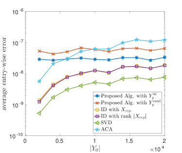
(a) $K_{1}(x,y)=1/|x-y|$

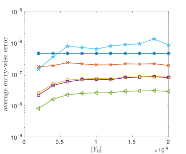
(b) $K_{2}(x,y)=\sqrt{1+|x-y|^{2}}$

Figure 8: Average entry-wise error of the obtained low-rank approximations.

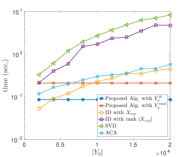
(a) $K_{1}(x,y)=1/|x-y|$

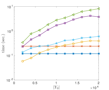
(b) $K_{2}(x,y)=\sqrt{1+|x-y|^{2}}$

Figure 9: Runtime of different low-rank approximation methods. The selection of $Y_{p}^{\text{id}}$ by Algorithm 1 takes $9.05$ sec. for $K_{1}(x,y)$ and $13.32$ sec. for $K_{2}(x,y)$.

For the two kernels, the average entry-wise errors of the proposed algorithm with $Y_{p}^{\text{id}}$ and $Y_{p}^{\text{rand}}$ both remain roughly constant for different $|Y_{0}|$ and are close to those of the ID approximation using sRRQR. The runtime of the proposed algorithm is independent of $|Y_{0}|$ which becomes advantageous over purely algebraic methods when $|Y_{0}|$ is large.

7.3 Comparison with different selections of $Y_{p}$

The number of points in both $Y_{p}^{\text{rand}}$ and $Y_{p}^{\text{surf}}$ need to be manually specified while Algorithm 1 determines the number of points in $Y_{p}^{\text{id}}$ automatically for different kernels and domain pairs. Intuitively, $|Y_{p}^{\text{id}}|$, as an estimate of $r_{KL}$, should be a good reference value for $|Y_{p}^{\text{rand}}|$ and $|Y_{p}^{\text{surf}}|$. Assuming that the proposed algorithm with $Y_{p}^{\text{id}}$ and the prescribed error threshold gives $K(X_{0},Y_{0})\approx W_{\text{rep}}K(X_{\text{rep}},Y_{0})$, we compare the rank-$|X_{\text{rep}}|$ ID approximations obtained by the proposed algorithm with following proxy point sets,

• $Y_{p}^{\text{rand}}$ with $\frac{1}{2}|Y_{p}^{\text{id}}|$, $|Y_{p}^{\text{id}}|$ and $2|Y_{p}^{\text{id}}|$ points.

• $Y_{p}^{\text{surf}}$ with $\frac{1}{2}|Y_{p}^{\text{id}}|$, $|Y_{p}^{\text{id}}|$ and $2|Y_{p}^{\text{id}}|$ points.

We continue to consider the far-apart domain pair in 3D and $X_{0}\in\mathcal{X}$ with 1000 points. Figure 10 shows the average entry-wise approximation error with different numbers of points in $Y_{0}$. The proxy-surface method (i.e., $Y_{p}^{\text{surf}}$) gives the best approximations for the 3D Laplace kernel $K_{1}(x,y)$ while its accuracy degrades drastically for the general kernel $K_{2}(x,y)$. Thus, the analytic method here leads to a better selection of the proxy points but the method is only limited to specific kernels and may be counter-productive otherwise.

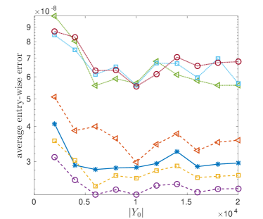
(a) $K_{1}(x,y)=1/|x-y|$

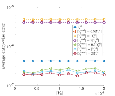
(b) $K_{2}(x,y)=\sqrt{1+|x-y|^{2}}$

Figure 10: Average entry-wise approximation error for two kernels with the far-apart domain pair in 3D. For $K_{1}(x,y)$, $|Y_{p}^{\text{id}}|=636$ and $|X_{\text{rep}}|=135$. For $K_{2}(x,y)$, $|Y_{p}^{\text{id}}|=821$ and $|X_{\text{rep}}|=142$.

Random Selection gives similar errors to that of ID Selection for both kernels, which can also be observed in Figure 8 of the previous test. This observation suggests that in some cases, Random Selection can be a better alternative of $Y_{p}^{\text{id}}$ since it requires no significant pre-calculation and it can be adapted to different domain pairs $\mathcal{X}\times\mathcal{Y}$ easily. However, it remains to decide a proper number of the points in $Y_{p}^{\text{rand}}$ since an insufficient number of points can lead to larger errors as can be somewhat suggested by Figure 10b and an excessive number of points can lead to more computation. Furthermore, we remind readers of the results in Section 7.1 that at some $y\in\mathcal{Y}$, the entry-wise error $e_{i}(y)$ can be 10 or more times larger than the expected error threshold $10^{-6}$. Thus, Random Selection can have much worse performance than ID Selection for $Y_{0}$ with specific point distributions.

More distinguishable differences between results from Random, ID and Surface Selection schemes can be found for the two kernels with the nearby domain pair in 2D as shown in Figure 11. In these results, it should be noted that for $K_{1}(x,y)$, all the $Y_{p}$ selections give much larger error than $10^{-6}$ while the rank-$|X_{\text{rep}}|$ truncated SVD for any of the tested $Y_{0}$ has average entry-wise error at most $10^{-7}$. The main cause of this accuracy degradation is the singularity of $K_{1}(x,y)$ when $x$ and $y$ are close. The analysis and solution for this problem will be explained in the next subsection.

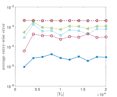
(a) $K_{1}(x,y)=1/|x-y|$

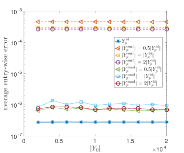
(b) $K_{2}(x,y)=\sqrt{1+|x-y|^{2}}$

Figure 11: Average entry-wise approximation error for two kernels with the nearby domain pair in 2D. For $K_{1}(x,y)$, $|Y_{p}^{\text{id}}|=500$ and $|X_{\text{rep}}|=197$. For $K_{2}(x,y)$, $|Y_{p}^{\text{id}}|=316$ and $|X_{\text{rep}}|=72$.

7.4 Improvement of the proxy point selection

Here, we introduce ideas to improve ID Selection. The ideas can be easily adapted to improve Random Selection. To better understand the large errors in Figure 11a, the average error function $\frac{1}{|X_{0}|-|X_{\text{rep}}|}\sum_{x_{i}\in X_{0}\backslash X_{\text{rep}}}|e_{i}(y)|$ over $\mathcal{Y}$ and the selected proxy point set $Y_{p}^{\text{id}}$ are drawn in Figure 12.

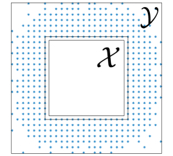
(a) Proxy point set $Y_{p}^{\text{id}}$ with 441 points in ${[-2,2]^{2}}$ and 59 points outside.

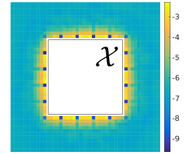
(b) $\frac{1}{|X_{0}|-|X_{\text{rep}}|}\sum_{x_{i}\in X_{0}\backslash X_{\text{rep}}}|e_{i}(y)|$ for ${y\in\mathcal{Y}}$ in $\log_{10}$ scale.

Figure 12: $Y_{p}^{\text{id}}$ obtained by Algorithm 1 and the associated error distribution in $\mathcal{Y}$, for $K_{1}(x,y)=\frac{1}{|x-y|}$ with the nearby domain pair in 2D. The plotted area is $[-2,2]^{2}$ to highlight differences. The error function values outside of $[-2,2]^{2}$ are approximately $10^{-7}$.

As can be observed, the largest errors are only located in the part of the domain near $\mathcal{X}$. The most likely cause is that $\frac{1}{|x-y|}$ varies rapidly when $x$ and $y$ become close, the candidate point set $Y_{d}$ in Algorithm 1 may not be dense enough in the area near $\mathcal{X}$ to satisfy the prerequisite that $\text{col}(\Phi(Y_{d}))=\mathbb{R}^{r_{KL}}$ in Equation 8. A hint towards this is that most of the candidate points near $\mathcal{X}$ are selected for $Y_{p}^{\text{id}}$.

A heuristic solution is to adaptively select more candidate points in the area where $K(x,y)$ has larger variation (e.g., according to $|\nabla_{y}K(x,y)|$). To test this idea, we uniformly select half of the candidate points, approximately 7500 points, from the small area $[2,2]^{2}\backslash[1.1,1.1]^{2}$ and the other half from the remaining large area $[9,9]^{2}\backslash[2,2]^{2}$. The corresponding results are shown in Figure 13. More proxy points ($|Y_{p}^{\text{id}}|=909$) are selected, especially from the area near $\mathcal{X}$, and the obtained average error also meets the expected accuracy at any $y\in\mathcal{Y}$. These results corroborate our explanation of the possible cause of the accuracy degradation. Alternatively, we can consider re-applying Algorithm 1 with denser initial candidates in areas with large error to improve the quality of proxy point set $Y_{p}^{\text{id}}$.

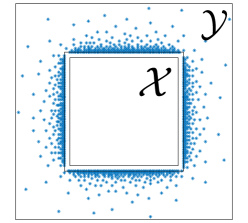
(a) Proxy point set $Y_{p}^{\text{id}}$ with 879 points in ${[-2,2]^{2}}$ and 30 points outside.

(b) $\frac{1}{|X_{0}|-|X_{\text{rep}}|}\sum_{x_{i}\in X_{0}\backslash X_{\text{rep}}}|e_{i}(y)|$ for ${y\in\mathcal{Y}}$ in $\log_{10}$ scale.

Figure 13: $Y_{p}^{\text{id}}$ obtained by Algorithm 1 with adaptively selected initial grid $Y_{d}$ and the associated error distribution in $\mathcal{Y}$, for $K_{1}(x,y)=\frac{1}{|x-y|}$ with the nearby domain case in 2D. The plotted area is $[-2,2]^{2}$. The error function values outside of $[-2,2]^{2}$ are approximately $10^{-7}$. The maximum average error over $\mathcal{Y}$ is found to be $7.97\times 10^{-7}$.

Note that in the weak admissibility setting, $K_{1}(x,y)$ is singular on the boundary between $\mathcal{X}$ and $\mathcal{Y}$ and no KL expansion exists for $K_{1}(x,y)$ over $\mathcal{X}\times\mathcal{Y}$. In this case, Algorithm 1 and the proposed algorithm no longer work. Practically, we can add a small gap between $\mathcal{X}$ and $\mathcal{Y}$ but $r_{\text{KL}}$ would be large and numerical tests show that large numbers of points for $Y_{d}$ and $Y_{p}^{\text{id}}$ are needed to achieve the same accuracy.

Another solution to both the accuracy degradation and the kernel singularity issue is inspired by the hybrid method in [16] and is illustrated in Figure 14. Consider $K_{1}(x,y)$ with the domain pair $\mathcal{X}\times\mathcal{Y}$ in 2D that satisfies the weak admissibility condition. Split $\mathcal{Y}$ into a neighboring field $\mathcal{Y}_{\text{near}}$ and a far field $\mathcal{Y}_{\text{far}}$. From the previous tests, the proposed algorithm works well for $\mathcal{X}\times\mathcal{Y}_{\text{far}}$ but does not work or has large error for $\mathcal{X}\times\mathcal{Y}_{\text{near}}$. For a target point set $Y_{0}\subset\mathcal{Y}$, split it as $Y_{0}=Y_{0}^{\text{near}}\cup Y_{0}^{\text{far}}$ so that $Y_{0}^{\text{near}}\subset\mathcal{Y}_{\text{near}}$ and $Y_{0}^{\text{far}}\subset\mathcal{Y}_{\text{far}}$. The idea is to only apply the proposed algorithm over $K_{1}(X_{0},Y_{0}^{\text{far}})$ and directly work on $K_{1}(X_{0},Y_{0}^{\text{near}})$. Specifically, denote $Y_{p,\text{far}}$ as some proxy point set selected for $K_{1}(x,y)$ over $\mathcal{X}\times\mathcal{Y}_{\text{far}}$ and find an ID approximation of $K_{1}(X_{0},Y_{0}^{\text{near}}\cup Y_{p,\text{far}})$ by sRRQR as

$$K_{1}(X_{0},Y_{0}^{\text{near}}\cup Y_{p,\text{far}})\approx W_{\text{rep}}K_{1}(X_{\text{rep}},Y_{0}^{\text{near}}\cup Y_{p,\text{far}}).$$

The ID approximation of $K_{1}(X_{0},Y_{0})$ is then defined as $W_{\text{rep}}K_{1}(X_{\text{rep}},Y_{0})$. In general, the splitting of $\mathcal{Y}$ should be kernel-dependent. This hybrid method will be illustrated in the next subsection on $\mathcal{H}^{2}$ construction.

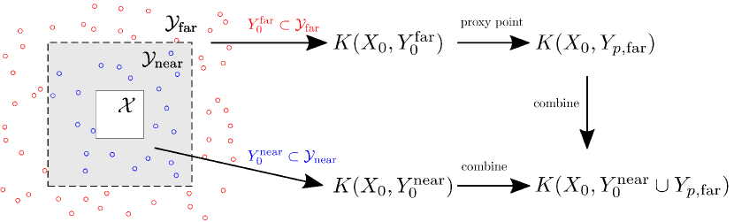
Figure 14: Hybrid variant of the proposed algorithm. Approximation of target matrix $K(X_{0},Y_{0})$ is obtained by an ID approximation of a smaller matrix $K(X_{0},Y_{0}^{\text{near}}\cup Y_{p,\text{far}})$ where $|Y_{p,\text{far}}|$ is not related to $|Y_{0}|$ and $|Y_{0}^{\text{near}}|$ is usually expected to be nearly constant in real problems.

7.5 $\mathcal{H}^{2}$ matrix construction

We now consider the ID-based $\mathcal{H}^{2}$ construction of symmetric kernel matrices $K(X,X)$ with some prescribed point set $X\subset\mathbb{R}^{d}$. The following two admissibility conditions are considered.

• strong admissibility condition: For any two non-adjacent boxes, the two enclosed point clusters are admissible.

• weak admissibility condition: For any two non-overlapping boxes, the two enclosed point clusters are admissible. The $\mathcal{H}^{2}$ matrix with this admissibility condition is usually called an HSS matrix in the literature.

The associated $\mathcal{H}^{2}$ representations are referred to as $\mathcal{H}^{2}_{\text{strong}}$ and $\mathcal{H}^{2}_{\text{weak}}$ respectively.

For problems in $\mathbb{R}^{d}$, to maintain constant point density, $N$ points are uniformly and randomly distributed in a box with equal edge length $L=N^{1/d}$. At the $k$th level of the hierarchical partitioning of the box, the sub-domains contain $2^{dk}$ boxes with edge length $L/2^{k}$. For the associated 1 at the $k$th level, set $\mathcal{X}=[-\frac{L}{2^{k+1}},\frac{L}{2^{k+1}}]^{d}$ and

$$\mathcal{Y}=\left\{\begin{array}[]{ll}[-(L-\frac{L}{2^{k+1}}),L-\frac{L}{2^{k+1}}]^{d}\setminus[-\frac{3L}{2^{k+1}},\frac{3L}{2^{k+1}}]^{d}&\text{ for }\mathcal{H}^{2}_{\text{strong}}\\ [-(L-\frac{L}{2^{k+1}}),L-\frac{L}{2^{k+1}}]^{d}\setminus\mathcal{X}&\text{ for }\mathcal{H}^{2}_{\text{weak}}\end{array}\right.,$$

based on the admissibility conditions.

For $\mathcal{H}^{2}_{\text{strong}}$ construction, the proposed algorithm with both ID and Random Selection schemes for $Y_{p}$ is compared with the ID approximation using sRRQR. $Y_{p}^{\text{id}}$ is selected by Algorithm 1 from a uniform initial set pair $X_{d}\times Y_{d}$ with approximately $1500\times 15000$ points and $Y_{p}^{\text{rand}}$ contains 2000 points in $\mathcal{Y}$.

For $\mathcal{H}^{2}_{\text{weak}}$ construction, the hybrid algorithm in Figure 14 with both Random and ID Selection schemes for $Y_{p,\text{far}}$ (denoted as $Y_{p,\text{far}}^{\text{rand}}$ and $Y_{p,\text{far}}^{\text{id}}$) is also tested. $\mathcal{Y}_{\text{far}}$, $Y_{p,\text{far}}^{\text{rand}}$ and $Y_{p,\text{far}}^{\text{id}}$ used in this algorithm are the same as $\mathcal{Y}$, $Y_{p}^{\text{rand}}$ and $Y_{p}^{\text{id}}$ in the $\mathcal{H}^{2}_{\text{strong}}$ construction case above. The non-hybrid version of the proposed algorithm for $K_{1}(x,y)$ is not tested due to the singularity of $K_{1}(x,y)$ on the boundary between $\mathcal{X}$ and $\mathcal{Y}$ in the weak admissibility setting. To select $Y_{p}^{\text{id}}$ for $K_{2}(x,y)$ by Algorithm 1, following the strategy from the previous subsection, half of the candidate points $Y_{d}$ are uniformly selected from a small area near $\mathcal{X}$ with the other half from the remaining large area. A similar strategy was used for $Y_{p}^{\text{rand}}$.

In the hierarchical partitioning, a sub-domain is subdivided when it has more than 300 points. For all the ID approximations in $\mathcal{H}^{2}$ construction, a relative error threshold of $\tau=10^{-6}$ is applied. We consider the two prescribed kernels in 2D. Figure 15 and Figure 16 show the runtime of our sequential Matlab implementation for $\mathcal{H}^{2}_{\text{strong}}$ and $\mathcal{H}^{2}_{\text{weak}}$ construction. Table 2 and Table 3 list some detailed data of these constructions.

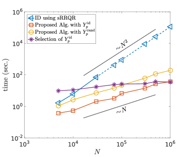
(a) $K_{1}(x,y)=1/|x-y|$

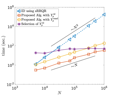
(b) $K_{2}(x,y)=\sqrt{1+|x-y|^{2}}$

Figure 15: Runtime of $\mathcal{H}^{2}_{\text{strong}}$ construction for two kernels in 2D. Construction with ID using sRRQR is not tested when $N\geqslant 70000$ due to memory limitations and the dashed lines indicate an extrapolation of the data.

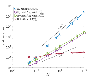
(a) $K_{1}(x,y)=1/|x-y|$

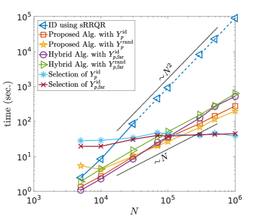
(b) $K_{2}(x,y)=\sqrt{1+|x-y|^{2}}$

Figure 16: Runtime of $\mathcal{H}^{2}_{\text{weak}}$ construction for two kernels in 2D. The dashed lines indicate an extrapolation of the data.

Table 2: Numerical results for $\mathcal{H}^{2}_{\text{strong}}$ construction. $\mathcal{S}$ denotes the storage cost (MB) of the obtained matrix representation. $\mathcal{E}$ denotes the relative error of the approximations of all compressed blocks. $\mathcal{S}$ or $\mathcal{E}$ with subscripts sRRQR, $Y_{p}^{\text{id}}$ and $Y_{p}^{\text{rand}}$ are the associated values obtained by the $\mathcal{H}^{2}$ construction using ID approximation using sRRQR, the proposed algorithm with $Y_{p}^{\text{id}}$ and that with $Y_{p}^{\text{rand}}$, respectively. $\mathcal{S}_{\text{N}}$ denotes the storage cost of the original dense matrix and $\mathcal{S}_{\text{inadm}}$ denotes the storage cost of the dense blocks in the $\mathcal{H}^{2}$ representation.

$K_{1}(x,y)=1/|x-y|$
$N$	$\mathcal{S}_{N}$	$\mathcal{S}_{\text{inadm}}$	$\mathcal{S}_{\text{sRRQR}}$	$\mathcal{S}_{Y_{p}^{\text{id}}}$	$\mathcal{S}_{Y_{p}^{\text{rand}}}$	$\mathcal{E}_{\text{sRRQR}}$	$\mathcal{E}_{Y_{p}^{\text{id}}}$	$\mathcal{E}_{Y_{p}^{\text{rand}}}$
5e3	1.9e2	25	35	39	37	6.9e-7	1.1e-6	1.5e-6
1e4	7.6e2	90	1.0e2	1.1e2	1.1e2	7.9e-7	1.2e-6	2.0e-6
3e4	6.9e3	2.2e2	2.9e2	3.1e2	2.7e2	9.1e-7	1.4e-6	5.7e-6
7e4	3.7e4	1.1e3	-	1.3e3	1.2e3	-	1.7e-6	1.9e-5
1e5	7.6e4	6.4e2	-	9.9e2	8.1e2	-	1.8e-6	6.9e-5
3e5	6.9e5	3.8e3	-	4.5e3	4.2e3	-	4.1e-6	1.4e-4
5e5	1.9e6	4.1e3	-	5.3e3	4.6e3	-	8.0e-6	2.1e-4
1e6	7.6e6	1.6e4	-	1.8e4	1.7e4	-	9.5e-6	2.0e-4

$K_{2}(x,y)=\sqrt{1+|x-y|^{2}}$
$N$	$\mathcal{S}_{N}$	$\mathcal{S}_{\text{inadm}}$	$\mathcal{S}_{\text{sRRQR}}$	$\mathcal{S}_{Y_{p}^{\text{id}}}$	$\mathcal{S}_{Y_{p}^{\text{rand}}}$	$\mathcal{E}_{\text{sRRQR}}$	$\mathcal{E}_{Y_{p}^{\text{id}}}$	$\mathcal{E}_{Y_{p}^{\text{rand}}}$
5e3	1.9e2	25	31	33	30	8.1e-7	4.4e-7	1.5e-6
1e4	7.6e2	90	97	1.0e2	97	8.8e-7	4.4e-7	1.2e-6
3e4	6.9e3	2.2e2	2.5e2	2.7e2	2.5e2	1.1e-6	4.7e-7	2.9e-6
7e4	3.7e4	1.1e3	-	1.2e3	1.2e3	-	5.0e-7	3.2e-6
1e5	7.6e4	6.4e2	-	8.0e2	7.1e2	-	4.9e-7	3.5e-6
3e5	6.9e5	3.8e3	-	4.2e3	3.9e3	-	4.7e-7	4.6e-6
5e5	1.9e6	4.1e3	-	4.7e3	4.3e3	-	5.1e-7	5.3e-6
1e6	7.6e6	1.6e4	-	1.7e4	1.7e4	-	5.1e-7	5.5e-6

Table 3: Numerical results for $\mathcal{H}^{2}_{\text{weak}}$ construction. Subscripts $Y_{p,\text{far}}^{\text{id}}$ and $Y_{p,\text{far}}^{\text{rand}}$ correspond to the hybrid algorithm with $Y_{p,\text{far}}^{\text{id}}$ and $Y_{p,\text{far}}^{\text{rand}}$ as the proxy point set for $\mathcal{Y}_{\text{far}}$ respectively. See the caption for Table 2 for the definitions of other notations.

$K_{1}(x,y)=1/|x-y|$
$N$	$\mathcal{S}_{N}$	$\mathcal{S}_{\text{inadm}}$	$\mathcal{S}_{\text{sRRQR}}$	$\mathcal{S}_{Y_{p,\text{far}}^{\text{id}}}$	$\mathcal{S}_{Y_{p,\text{far}}^{\text{rand}}}$	$\mathcal{E}_{\text{sRRQR}}$	$\mathcal{E}_{Y_{p,\text{far}}^{\text{id}}}$	$\mathcal{E}_{Y_{p,\text{far}}^{\text{rand}}}$
5e3	1.9e2	3.9	28	29	29	6.2e-6	1.8e-6	5.7e-7
1e4	7.6e2	12	67	69	69	8.9e-6	3.4e-6	1.1e-6
3e4	6.9e3	27	2.7e2	2.7e2	2.7e2	1.1e-5	3.8e-6	1.7e-6
7e4	3.7e4	1.4e2	-	7.9e2	7.9e2	-	4.6e-6	2.6e-6
1e5	7.6e4	75	-	1.1e3	1.2e3	-	5.5e-6	3.0e-6
3e5	6.9e5	4.8e2	-	4.3e3	4.3e3	-	7.1e-6	4.6e-6
5e5	1.9e6	4.7e2	-	7.6e3	7.6e3	-	1.0e-5	7.2e-6
1e6	7.6e6	1.9e3	-	1.7e4	1.7e4	-	1.3e-5	9.4e-6

$K_{2}(x,y)=\sqrt{1+|x-y|^{2}}$
$N$	${}^{\ast}\mathcal{S}_{\text{sRRQR}}$	$\mathcal{S}_{Y_{p}^{\text{id}}}$	$\mathcal{S}_{Y_{p}^{\text{rand}}}$	$\mathcal{S}_{Y_{p,\text{far}}^{\text{id}}}$	$\mathcal{S}_{Y_{p,\text{far}}^{\text{rand}}}$	$\mathcal{E}_{\text{sRRQR}}$	$\mathcal{E}_{Y_{p}^{\text{id}}}$	$\mathcal{E}_{Y_{p}^{\text{rand}}}$	$\mathcal{E}_{Y_{p,\text{far}}^{\text{id}}}$	$\mathcal{E}_{Y_{p,\text{far}}^{\text{rand}}}$
5e3	15	37	23	17	15	1.7e-6	6.5e-7	1.4e-6	1.3e-6	3.3e-6
1e4	33	86	47	41	34	1.9e-6	8.2e-7	3.5e-6	1.2e-6	3.0e-6
3e4	94	3.0e2	1.0e2	1.4e2	1.0e2	2.6e-6	8.7e-7	7.0e-6	1.7e-6	3.4e-6
7e4	-	7.6e2	2.6e2	4.0e2	3.3e2	-	1.0e-6	1.3e-5	2.1e-6	2.9e-6
1e5	-	1.0e3	2.2e2	5.0e2	3.5e2	-	1.1e-6	1.5e-5	2.1e-6	3.5e-6
3e5	-	3.1e3	7.6e2	1.8e3	1.3e3	-	4.5e-6	2.1e-5	2.7e-6	3.4e-6
5e5	-	4.9e3	8.0e2	2.7e3	1.7e3	-	3.6e-6	2.3e-5	2.7e-6	3.7e-6
1e6	-	9.9e3	2.4e3	6.3e3	4.3e3	-	5.4e-6	2.4e-5	3.3e-6	3.5e-6

^∗Refer to the table for $K_{1}(x,y)$ for values of $\mathcal{S}_{N}$ and $\mathcal{S}_{\text{inadm}}$.

For both constructions, the runtime of the pre-calculation for $Y_{p}^{\text{id}}$ is significant but its asymptotic complexity is only $O(\log(N))$ as the selection of $Y_{p}^{\text{id}}$ is only performed once for each level. Both the proposed and hybrid algorithms lead to nearly linear $\mathcal{H}^{2}$ construction which can also be verified by complexity analysis if we assume that the maximum rank of the low-rank off-diagonal blocks and the number of points in $Y_{p}$ for each level are both of constant scale. Also, $\mathcal{H}^{2}$ construction with these two algorithms has larger storage cost compared to that with ID using sRRQR because, as explained earlier, they generally select more rows in the ID approximation.

For $\mathcal{H}^{2}_{\text{strong}}$ construction, the proposed algorithm with $Y_{p}^{\text{rand}}$ takes more time since $Y_{p}^{\text{rand}}$ has more points than $Y_{p}^{\text{id}}$ which contains approximately 900 points for each level. The relative errors of $\mathcal{H}^{2}_{\text{strong}}$ and $\mathcal{H}^{2}_{\text{weak}}$ approximations for $K_{1}(x,y)$ both increase with larger $N$ which can be observed for both proxy point selection schemes and for both the proposed algorithm and the ID using sRRQR. This is mainly due to the amplification of errors at the level-by-level $\mathcal{H}^{2}$ construction and is also kernel-dependent. The hierarchical partitioning trees have $4,4,5,6,6,7,7,7$ levels for the values of $N$ tested, which roughly matches the incremental pattern of the errors in Table 2.

For $\mathcal{H}^{2}_{\text{weak}}$ construction, the hybrid algorithms with both selection schemes for $Y_{p}$ are effective and provide good approximations. In addition, for $K_{2}(x,y)$, the hybrid algorithm has less storage cost (i.e., smaller ranks for ID approximations) and similar or even smaller relative errors compared to the non-hybrid algorithm with $Y_{p}^{\text{id}}$. This advantage of the hybrid algorithm is expected since the hybrid algorithm directly works on a part of $Y_{0}$ in the ID approximation.

8 Conclusion

We proposed an efficient low-rank approximation algorithm for the sub-blocks of kernel matrices that can also be regarded as a generalization of the proxy-surface method. For the proposed algorithm, two proxy point selection schemes were introduced in Section 5 as well as two heuristic improvements to the schemes in Section 7.4. The two proxy point selection schemes that were introduced are general in that they can be applied to any kernel and any domain pair. It should be possible to design specialized selection schemes that are kernel-dependent and thus are more effective than the general schemes, as long as condition Equation 8 is met. In practice, the algorithm can be used for hierarchical matrix construction for general translation-invariant kernels to give a construction cost linear in the matrix dimension if the maximum rank of the low-rank off-diagonal blocks does not increase with the matrix dimension.

References

- [1] Sivaram Ambikasaran and Eric Darve. An Fast Direct Solver for Partial Hierarchically Semi-Separable Matrices. Journal of Scientific Computing, 57(3):477–501, December 2013.
- [2] M. Bebendorf and S. Rjasanow. Adaptive Low-Rank Approximation of Collocation Matrices. Computing, 70(1):1–24, February 2003.
- [3] Mario Bebendorf. Approximation of boundary element matrices. Numerische Mathematik, 86(4):565–589, October 2000.
- [4] Cai, Difeng, Chow, Edmond, Saad, Yousef, and Xi, Yuanzhe. SMASH: Structured matrix approximation by separation and hierarchy. eprint arXiv:1705.05443, May 2017.
- [5] S. Chandrasekaran, M. Gu, and T. Pals. A Fast ULV Decomposition Solver for Hierarchically Semiseparable Representations. SIAM Journal on Matrix Analysis and Applications, 28(3):603–622, January 2006.
- [6] H. Cheng, Z. Gimbutas, P. Martinsson, and V. Rokhlin. On the Compression of Low Rank Matrices. SIAM Journal on Scientific Computing, 26(4):1389–1404, January 2005.
- [7] L Greengard and V Rokhlin. A fast algorithm for particle simulations. Journal of Computational Physics, 73(2):325–348, December 1987.
- [8] Leslie Greengard and Vladimir Rokhlin. A new version of the Fast Multipole Method for the Laplace equation in three dimensions. Acta Numerica, 6:229–269, January 1997.
- [9] M. Gu and S. Eisenstat. Efficient Algorithms for Computing a Strong Rank-Revealing QR Factorization. SIAM Journal on Scientific Computing, 17(4):848–869, July 1996.
- [10] W. Hackbusch. A Sparse Matrix Arithmetic Based on -Matrices. Part I: Introduction to -Matrices. Computing, 62(2):89–108, April 1999.
- [11] W. Hackbusch and S. Börm. Data-sparse Approximation by Adaptive -Matrices. Computing, 69(1):1–35, September 2002.
- [12] W. Hackbusch, B. Khoromskij, and S. A. Sauter. On -Matrices. Lectures on Applied Mathematics, pages 9–29, 2000.
- [13] W. Hackbusch and B. N. Khoromskij. A Sparse -matrix Arithmetic. Part II: Application to Multi-dimensional Problems. Computing, 64(1):21–47, January 2000.
- [14] W. Hackbusch and Z. P. Nowak. On the fast matrix multiplication in the boundary element method by panel clustering. Numerische Mathematik, 54(4):463–491, July 1989.
- [15] N. Halko, P. Martinsson, and J. Tropp. Finding Structure with Randomness: Probabilistic Algorithms for Constructing Approximate Matrix Decompositions. SIAM Review, 53(2):217–288, January 2011.
- [16] K. Ho and L. Greengard. A Fast Direct Solver for Structured Linear Systems by Recursive Skeletonization. SIAM Journal on Scientific Computing, 34(5):A2507–A2532, January 2012.
- [17] P. Martinsson. A fast randomized algorithm for computing a hierarchically semiseparable representation of a matrix. SIAM Journal on Matrix Analysis and Applications, 32(4):1251–1274, 2011.
- [18] P. G. Martinsson and V. Rokhlin. A fast direct solver for boundary integral equations in two dimensions. Journal of Computational Physics, 205(1):1–23, May 2005.
- [19] Lexing Ying, George Biros, and Denis Zorin. A kernel-independent adaptive fast multipole algorithm in two and three dimensions. Journal of Computational Physics, 196(2):591–626, May 2004.