[figure]footposition=caption

Deep Learning Super-Diffusion in Multiplex Networks

Abstract

Complex network theory has shown success in understanding the emergent and collective behavior of complex systems Newmanbook . Many real-world complex systems were recently discovered to be more accurately modeled as multiplex networks GinestraBook ; BOCCALETTI20141 ; Lee2015 ; Kivela2014 ; MultNetMathPRX —in which each interaction type is mapped to its own network layer; e.g. multi-layer transportation networks, coupled social networks, metabolic and regulatory networks, etc. A salient physical phenomena emerging from multiplexity is super-diffusion: exhibited by an accelerated diffusion admitted by the multi-layer structure as compared to any single layer. Theoretically super-diffusion was only known to be predicted using the spectral gap of the full Laplacian of a multiplex network and its interacting layers. Here we turn to machine learning which has developed techniques to recognize, classify, and characterize complex sets of data. We show that modern machine learning architectures, such as fully connected and convolutional neural networks, can classify and predict the presence of super-diffusion in multiplex networks with 94.12% accuracy. Such predictions can be done in situ, without the need to determine spectral properties of a network.

Complex systems are often well-approximated by complex networks or graphs, i.e. elements of the system can be represented as nodes where connections between nodes correspond to non-trivial interaction patterns Newmanbook ; EstradaBook . A multiplex (multi-layer) network is a generalized framework to study complex networks with more than one interacting layer: each layer represents a different type of interaction between constituent nodes GinestraBook ; BOCCALETTI20141 ; Lee2015 ; Kivela2014 ; MultNetMathPRX . Vast efforts have only more recently been devoted to study the differences and new phenomenon in networks when multiplexity is taken into account Szell2010 ; Mucha2010 . By considering multiplexity, a network becomes a so called multi-layer structure—thereby aggregating all layers into one single-layer network, or considering each layer separately typically entails a lossy compression MultNetMathPRX .

Considering multiplexity has lead to the discovery of new behavior in networked systems. The seminal paper by Buldyrev Buldyrev2010 proves multiplex networks (interdependent networks in their case) exhibit a first order abrupt phase transition in their percolation phase diagram. This finding is in contrast to continuous phase transitions exhibited in the percolation phase diagram of monoplex networks (single-layer networks) Cohen2000PRL ; Newman2003Siam . Then numerous papers tried to understand different behaviors that arise in studying multilayer graphs. Examples include, structural processes such as site, bond percolation Hackett2016PRX ; Bianconi2016PRE ; Cellai2013PRE ; Radicchi2015NatPhys ; RadicchiBianconi2017PRX ; ghavasieh2020unraveling , first-depth percolation or observability, kcore AzimiKcore2014PRE , optimal percolation Osat2017NatComm , as well as dynamical processes such as epidemic spreading DickisonEpidemic2012PRE , synchronization Genio2016SciAdv , diffusion DeDomenico2014PNAS ; GomezSupDiff2013PRL ; Tejedor2018PRX , controllability Posfai2016PRE and recently multi-dynamics running on top of multilayer structures WANG2015LIFE ; Granell2013PRL ; Granell2014PRE ; Lima2015 ; AzimiEpidemic2016PRE . Here we focus on super-diffusion—a physically observed phenomena in which a coupling between two distinct types of networks, creates ‘shortcuts’ e.g. using a bus and then a metro can result in crossing town much faster than relying on either buses or the metros alone.

Conventionally, multiplex networks and particularly super-diffusion has been studied using a variety of tools from statistical physics, spectral graph theory and other tailored methods which are paired with powerful computer simulations and/or numerical methods GinestraBook . The computer simulations are case dependent; e.g. Monte Carlo sampling is used to study percolation, or simulation of epidemic spreading, whereas spectral methods are related to some specific problems including community detection, percolation threshold, combinatorial problems, etc. A specific (yes/no) question answered using spectral graph theory is the presence of super-diffusion in a given multiplex network. In current approaches, the spectral gap of the graph Laplacian—the first non-trivial eigenvalue of the Laplacian—is calculated to determine whether a multiplex system exhibits super-diffusion or not GomezSupDiff2013PRL .

Machine learning has been successfully applied in a number of complex networks studies MLCompNet . This includes hyperbolic embedding of complex networks Muscoloni2017NatComm , link prediction Hasan06linkprediction and representation learning Hamilton2017RepresentationLO . However, augmenting the tool-set of complex networks with modern deep learning approaches is still in its nascent stages, with work reporting link prediction LinkML2018 . The ability of modern machine learning techniques to classify, identify, and/or interpret massive data sets such as images foreshadows their suitability to provide network scientists with similar success cases when studying the extremely large data sets embodied in the state-space of complex networks.

In this study, we employ a deep learning approach which trains a neural network to (successfully) classify the presence of super-diffusion phenomena in multiplex networks. We represent the data-set in a gray-scale image and employ two different neural network architectures from machine learning (multilayer perceptron) and deep learning (convolutional neural network goodfellow2016deep , lecun1998gradient ). Definitively, our trained neural networks predict super-diffusion in multiplex networks with 94.12% accuracy. Such predictions can be done in situ, without the need of a networks spectral properties. We believe that the success of this finding will foster a wide application of deep learning to study complex networks.

Super-diffusion.

Diffusion processes are among the simplest dynamics studied on multiplex structures GomezSupDiff2013PRL . Gomez et al. GomezSupDiff2013PRL studied diffusion in a duplex (two layer multiplex network) and found out that under certain circumstances, diffusion can be faster in a multiplex network compared to diffusion in each of the layers separately GomezSupDiff2013PRL . This phenomena—which is called super-diffusion in multiplex networks—can be predicted by leveraging the relation between the spectrum of a Laplacian matrix and diffusion time-scales. The combinatorial Laplacian (as called in graph theory) governs dynamics of diffusion running on top of the graph i.e. the Laplacian is the generator of the stochastic process describing the random walk on the graph. While there are fundamental connections between the spectrum of the Laplacian of a graph with structural properties of a graph itself, there are also relationships between the spectrum and dynamics running on top of the graph. In the case of diffusion processes, the second smallest eigenvalue (the first nontrivial one) of the Laplacian controls the timescale of the diffusion process. In the case of multiplex networks, the Laplacian matrix has the counterpart which is called supra-Laplacian MultNetMathPRX which is the same as the Laplacian matrix yet offers an easier interpretation (with proper labeling of nodes) as a block diagonal matrix in which diagonal blocks are the Laplacian of each of the layers (capturing intra-layer connections) and off-diagonal blocks which capture interlayer connections.

$$\mathcal{L}(\mathcal{L}_{1},\mathcal{L}_{2},w)=\left(\begin{array}[]{cc}\mathcal{L}_{1}+w\openone&-w\openone\\ -w\openone&\mathcal{L}_{2}+w\openone\end{array}\right)$$ (1)

Gomez et al. GomezSupDiff2013PRL showed that strength of interlayer connections ($w$) is a tunable parameter between slow and fast diffusion regimes. For weak inter-layer connections, multiplexity slows down the diffusion while strong inter-layer connections define a new behavioral regime which asymptotically approaches the behavior of the aggregated layer (the superposition of the two layers). In the strong coupling regime, if

$$\lambda_{2}(\mathcal{L})\geq\text{Max}\{\lambda_{2}(\mathcal{L}_{1}),\lambda_{2}(\mathcal{L}_{2})\}$$ (2)

super-diffusion is exhibited or in other words, multiplexity helps diffusion happen faster. These two distinct regimes are direct consequence of structural transitions in the formation of multiplex networks starting from separate layers and then placing inter-layer links between them and increasing the weight of these links Radicchi2013NatPhys ; Radicchi2018PRX ; Rapisardi2018PRE ; Darabi2015PRE ; MARTINHERNANDEZ201492 . The phenomena was also reported recently for directed multiplex networks Tejedor2018PRX .

De Domenico et al. DeDomenico2016NatPhys numerically tested for the super-diffusion phenomena on multiplex networks composed of two layers which first and second layers are Erdős-Rényi random graphs from $\mathcal{G}(N,p_{1})$ and $\mathcal{G}(N,p_{2})$ respectively, in which, $\mathcal{G}(N,p)$ is the classical random graph ensemble which there are $N$ nodes and each pair of the nodes are connected with probability $p$. They found out that super-diffusion in these specific multiplexes happens mostly in the same connection probability regime ($p_{1}\approx p_{2}$) DeDomenico2016NatPhys . For a multiplex that its layers are generated with very different probabilities, multiplexity or having multilayer structure has no benefits in terms of diffusion timescale and hence, diffusion in at least one of the layers when considered independently will be faster than this connected multiplex. Fig. 1 shows the phenomena of super-diffusion and its phase diagram on random multiplex networks.

While the super-diffusion phase diagram achieved using numerical test, the following question is legitimate: is it possible to design a machine learning algorithm to detect presence of super-diffusion given a multiplex network? To answer this question we propose a supervised ML algorithm.

Deep Learning.

Machine learning (ML), particularly deep learning is now the standard tool in many different areas: from computer vision  lecun1998gradient ; goodfellow2016deep ; krizhevsky2012imagenet ; simonyan2014very ; szegedy2015going ; he2016deep to condensed matter physics  Carrasquilla2017NatPhys ; vanNieuwenburg2017NatPhys ; carleo2017solving ; Chng2017PRX ; Wetzel2017PRE ; Wenjian2017PRE and quantum systems Torlai2018NatPhys ; Biamonte2017Nature ; Deng2017PRX ; Zhang2017PRL . Application of complex networks to different ML areas has a long story for supervised learning  Bertini2011 , unsupervised learning  Karypis1999 , semi-supervised learning Chapelle2006 . Instead of using complex networks to study deep neural networks, in this paper we present the converse: i.e. we apply ML methods to study complex networks.

Which neural network structures are most suited to predict super-diffusion in multiplex networks? To this end the following architectures of Artificial Neural Networks (ANN) were applied: (1) fully connected neural networks (FCNN) with $l_{2}$ regularization; (2) FCNN with dropout and (3) convolutional neural networks (CNN). The realization was implemented using Keras API Keras backed by TensorFlow tensorflow2015-whitepaper .

Training Set.

We consider duplexes—multiplex networks with two layers (see appendix 2 for the generalization of the framework for multiplex networks with more than two layers). Both the first and second layers have exactly $N$ nodes and are created independently according to the Erdős-Rényi random graph model: $\mathcal{G}(N,p_{1})$ and $\mathcal{G}(N,p_{2})$ respectively. In the $\mathcal{G}(N,p)$ model, a graph is constructed (here each graph forms one duplex layer) by connecting nodes randomly. Each edge is included in the graph with probability $p$ independent from every other edge. Equivalently, all graphs with $N$ nodes and $M$ edges have equal probability of

$$p^{M}(1-p)^{\binom{N}{2}-M}.$$ (3)

Here the parameter $p$ in this model can be thought of as a weighting function—as $p$ increases from 0 to 1, the model becomes more and more likely to include graphs with increasing numbers of edges and increasingly less likely to include graphs with fewer edges. In particular, the case $p=1/2$ corresponds to the case where all $2^{\binom{N}{2}}$ graphs on $N$ nodes are chosen with equal probability.

Both layers are undirected and unweighted graphs. Connection patterns are encoded in an adjacency matrix $\mathcal{A}^{[1]}~{}(\mathcal{A}^{[2]})$ for the first (second) layer, where $\mathcal{A}^{[1]}_{ij}=1$ (and then $\mathcal{A}^{[2]}_{ij}=1$) if there is a link between node $i$ and node $j$ (all intra-layer links have weights equal to 1). Then we connect these two identical layers by one-to-one interlayer links each with non-negative weight $w$. According to GomezSupDiff2013PRL ; Radicchi2013NatPhys , changing the interlayer weights enables one to explore monoplex-multiplex regimes.

We divide the $p_{1}$-$p_{2}$ phase diagram into bins with $\delta p=0.02$ for the training phase and $\delta p=0.01$ in the testing phase. For each bin, we create $30$ training and $20$ test sample multiplex networks $(\mathcal{G}(N,p_{1}),\mathcal{G}(N,p_{2}))$. If super-diffusion will be exhibited

$$\lambda_{2}(\mathcal{L}^{sup})\geq\text{Max}\{\lambda_{2}(\mathcal{L}_{1}),\lambda_{2}(\mathcal{L}_{2})\}$$ (4)

then we label the input set $\{\mathcal{A}^{[k]},\mathcal{A}^{[m]},\dots\}$ as 1, and otherwise with 0.
We generated $75,000$ random graph instances for the training set and $200,000$ instances for the test set.

Fully connected neural networks for super-diffusion prediction.

To feed our data to fully connected neural network we make the following transformation. Since adjacency matrices are symmetric $N\times N$ with zeros on the diagonal, we can represent multiplex networks as a matrix with an upper triangle equal to the upper triangle of the first layer and a lower triangle equal to the lower triangle of the second layer. Then this matrix can be reshaped to a $N^{2}\times 1$ column matrix.

To test the quality recovered from use of a fully connected neural network (FCNN) we choose a simple architecture which consists of one input layer, one hidden layer and one output layer with two neurons. The activation function of the hidden layer is the so-called, ReLU (Rectified Linear Unit) function. To use our FCNN as a classifier, the output layer is activated by a sigmoid function. For the first FCNN model, the loss function was chosen as average cross-entropy between predicted and actual values with additional $l_{2}$ regularization term to prevent over-fitting. The optimization procedure of the loss function was done by the extension to stochastic gradient descent DBLP:journals/corr/KingmaB14 .

The resulting accuracy of the model is $93\%$ on the test data. The FCNN with dropout recovers the same result.

To reconstruct Fig. 1 we plot the distribution of the predicted result. The results are presented in Fig. 2 (b) and (c). We notice that the shape of the distributions varies for real super-diffusion (a) particularly for the left-down and up-right corners of the plot.

Convolutional neural networks for super-diffusion prediction.

The design of convolutional neural networks (CNN) which we utilized for the problem is shown on Fig. 3. The input of the CNN is two channel $50\times 50$ binary image followed by two convolutional layers with a small size $5\times 5$ filters and pooling layers. The result is flattened and connected to FCN with two outputs with preceding activation sigmoid function.

To feed data to the CNN we represented the 2 separated adjacency matrices of a multiplex network as binary images of 50 by 50 pixels and assigned those as two separated channels on the input layer. This procedure is shown on the left side of Fig. 3.

Interestingly enough the resulting accuracy $94\%$ is slightly better for the CNN then for FCNN and the shape of the distribution of predicted result looks more similar to the real distribution Fig. 2(d-f). This fact points out that the representation of a multiplex network as a multi-channel image for CNNs inputs is quite promising feature to investigate properties of multiplexes. And probably more complicated CNN’s architectures could perform better results. See appendix 1 for more information on the accuracy of the results predicted by CNN.

Conclusions.

We have found that convolutional neural network technology, developed for applications such as computer vision, can be used to detect super-diffusion in multiplex networks. We argue that this idea is quite natural and likely can attribute some of its success due to our representation of a multiplex layers adjacency matrix as channels of an image.

While traditional machine learning techniques have long been part of the complex networks tool-kit, deep learning is in its nascent days of application. Indeed, two-layer FCN was used as perhaps the simplest example of deep neural network, likewise with our simplistic simple CNN structure ($l_{2}$ regularization and drop-out techniques were used to prevent over fitting). In both cases, training resulted in high detection probability, thereby confirming proof of principle even for simplistic neural network architectures (over $94\%$ accuracy).

Based on our findings, we however anticipate a further use of deep learning in the field of complex networks, such as detecting phase transitions, and network dismantling. Interestingly, the application of complex networks as a tool to study properties of supervised learning  Bertini2011 , unsupervised learning  Karypis1999 and semi-supervised learning Chapelle2006 has long been considered. By applying deep learning to study properties of complex networks we then hope to form a bridge and a future where these two subjects compliment each other with deep learning regularly applied to complex networks.

As mentioned, the main property of multiplex networks which appears useful and quite natural for CNN, is the adjacency matrix which can be represented as data-set for every layer. This has the same format as image channels and is likely accountable as to why CNN filters can detect features responsible for super-diffusion in multiplex networks so readily.

Appendix 1

Here we show some metrics obtained by a cross validation where we divided the whole set in 10 stratified folds (each preserve the percentage of samples for both classes). For every step we kept 9 folds for training and 1 for testing. Fig. 5 shows the ROC curve (receiver operating characteristic curve) of the different folds and the mean AUC (area under the ROC curve) of 98%. The average accuracy obtained from the different folds is 94%. Table Deep Learning Super-Diffusion in Multiplex Networks shows the confusion matrices for K-Fold validation (top) and for the independent test set (bottom). Fig 5 shows the loss curve for the 10-fold stratification over 40 epochs, as additional metrics we generated heatmaps for each epoch and measured against the ground truth with Mean Squared Error and Structural Similarity Index with results shown in Table 5.

Appendix 2

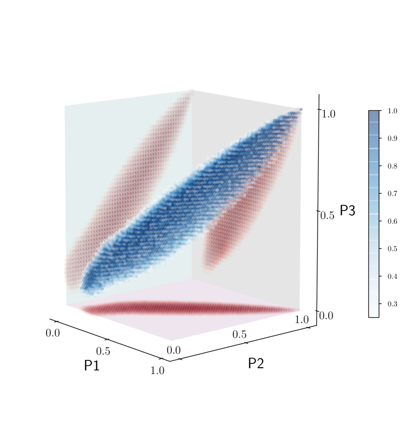
Figure 6: (Generalizing to more than two layers.) Predicted super diffusion phase diagram in 3-layer random multiplex networks. Each layer is an Erdős-Rényi random graph sampled from $\mathcal{G}(N,p)$ ensemble, where $N$ is number of nodes ($N=50$) and $p$ is the connection probability. For each ($p_{1},p_{2},p_{3}$) we create 20 samples of the 3-layer random multiplex networks, then we check the condition of super-diffusion on each of them. Color coding is based on the probability of the existence of super diffusion in each bin. For clarity we kept only data points corresponding to probabilities higher than 0.5. Projections of the main heatmap in (x,y), (x,z) and (y,z) planes represent the super diffusion in corresponding sub-duplexes formed by different combinations of layers. The only change in the DNN architecture is the input layer which is composed of three channels (the complete input shape is [50 x 50 x 3]). The classification accuracy obtained is 94%

Here we extend the framework presented in the main text to 3-layer multiplex networks (feeding CNN with adjacency matrices of the layers and following training procedure as explained in the main text). Fig. 6 shows the ability of our deep learning framework to predict super diffusion in case of multiplex networks with more than two layers. This proves the extension feasibility of the machinery to higher order multiplex networks. In the case of multiplex networks with three layers, We divide the $p_{1}$-$p_{2}$-$p_{3}$ phase diagram into bins with $\delta p=0.020$. For each bin we create $15$ training samples multiplex networks $(\mathcal{G}(N,p_{1}),\mathcal{G}(N,p_{2}),\mathcal{G}(N,p_{3}))$. If super-diffusion will be exhibited

$$\lambda_{2}(\mathcal{L}^{sup})\geq\text{Max}\{\lambda_{2}(\mathcal{L}_{1}),\lambda_{2}(\mathcal{L}_{2}),\lambda_{2}(\mathcal{L}_{3})\}$$ (5)

then we label the input set $\{\mathcal{A}^{[k]},\mathcal{A}^{[m]},\dots\}$ as 1, and otherwise with 0.
We generated $100,000$ random graph instances for the training set and $50,000$ instances for the test set (the latter has same $\delta p=0.020$ and $20$ samples per bin). Fig 6 shows the resulting heatmap on test set.

Appendix 3

Here we extend the framework presented in the main text to 2-layer multiplex networks of arbitrary $N$ nodes. We found that the original architecture can be extended to correctly classify bigger multiplex by stacking successive convolution (Conv) and pooling (Pool) layers. In the original $N=50$ size we stacked two Conv plus Pool layers, the only change in the DNN architecture is the number of Conv plus Pool layers, The number of such stacks is $\lceil N\bmod 50\rceil+1$. Each layer is an Erdős-Rényi random graph sampled from $\mathcal{G}(N,p)$ ensemble, where $N$ is number of nodes ($N=50,100,150,200,250,300,350,400,450$ and $500$) and $p$ is the connection probability. Likewise the $N=50$ case, we divide the training set in bins of $\delta p=0.002$ and the test set with $\delta p=0.001$, we create 30 samples per bin in train and 20 in test sets.

Data availability.

The data that support the plots within this paper and other findings of this study as well as all source code are available online.

Figure 1: (Super-Diffusion in multiplex networks.) A heat map of super-diffusion in the whole phase diagram of 2-layer multiplex networks was created, in which each layer has been formed using the Erdős-Rényi random graph model $\mathcal{G}(N,p)$, where $N$ is number of nodes ($N=50$) and $p$ is the connection probability. For each ($p_{1},p_{2}$) we create 10 samples of the 2-layer random multiplex networks, then we check the condition of super-diffusion; $\lambda_{2}(\mathcal{L})\geq\text{Max}\{\lambda_{2}(\mathcal{L}_{1}),\lambda_{2}(\mathcal{L}_{2})\}$ and then color code the probability of the super-diffusion for the bin ($p1,p2$). The plot indicates that super-diffusion happens mainly in the region that connections probabilities are close to each other. The left (right) zoomed window shows the whole phase diagram of $\lambda_{2}(\mathcal{L})$ for the case that super-diffusion happens (does not happen). Vertical yellow line in the zoomed windows represents the phase transition point: ($p^{*}=\frac{1}{2}\lambda_{2}(Q)$ where $Q=\mathcal{L}_{1}\bar{\mathcal{L}}^{\dagger}\mathcal{L}_{2}$ and $\bar{\mathcal{L}}^{\dagger}$ is the Moore-Penrose pseudoinverse of $\bar{\mathcal{L}}=\frac{\mathcal{L}_{1}+\mathcal{L}_{2}}{2}$) [38]. The circular layout of networks are shown in color-code based on Fiedler vectors of $\mathcal{L}$ which is the eigenvector corresponding to the spectral gap; before the transition point networks are decoupled and after transition point they are coupled [36].

Figure 2: (Machine learning super-diffusion.) Heatmap formed from averaging of ideal super-diffusion over (a) test data and predictions with (b) FCN with dropout, (c) FCN with l2 regularization, (d) CNN at first, (e) at fifth (f) and at twentieth epoch . Those heatmaps are just for data visualization, each p1-p2 square (with $\delta p=0.01$) contains the percentage of super-diffusion classified instances, The Structural Similarity with the ground truth (a) are 91% (b), 88.9% (c), 89.9% (d), 90.5% (e) and 92% (f).

Figure 3: (Deep neural network architecture detecting super-diffusion.) Two-layer random multiplex instances were randomly generated; each layer was generated independently from random graph model $\mathcal{G}(N,p)$, which $N$ is the number of nodes ($=50$) and $p$ is the connection probability. Adjacency matrices of each layer is represented as binary images of $50\times 50$ and then fed to the CNN as two separated channels ($\mathcal{A}^{[1]}$, $\mathcal{A}^{[2]}$) (the complete input shape is [$50\times 50\times 2$]). A first convolution (CONV1) is performed using a $5\times 5$ filter, same padding, ReLU activation function and 32 channels (the output shape is [$50\times 50\times 32$]). One max pooling layer (POOL1) is used to half the input shape with window size of $2\times 2$ and same padding (resulting in the shape of [$25\times 25\times 32$]). The second convolution (CONV2) has the same properties of (CONV1) except for the number of channels—growing now to 64 (shape of [$25\times 25\times 64$]). After a second max pooling layer (POOL2) that has the same properties of (POOL1) the resulting data (of shape [$13\times 13\times 64$]) is flattened to a single vector (of [10816] elements) and fed to a fully connected layer (of [1024] nodes) and to an final output layer (with [1] output node). The output is as a binary classifier which determines if the instance exhibits super diffusion or not.

Positive	Negative
Positive	$1602.1\quad$	$291.7\quad$	PPV = $0.85\pm 0.04$
Negative	$385.9\quad$	$8819.3\quad$	NPV = $0.96\pm 0.01$
	TPR = $0.81\pm 0.06$	TNR = $0.97\pm 0.01$
	(Sensitivity)	(Specificity)

Positive	Negative
Positive	$30193\quad$	$5494\quad$	$PPV=0.85$
Negative	$6772\quad$	$157541\quad$	$NPV=0.96$
	TPR = $0.82\hskip 14.22636pt$	TNR = $0.97$
	(Sensitivity)	(Specificity)

Figure 4: (Performance of SD detection (ROC curves)) Cross-validation on a stratified 10-fold data. Two datasets with different partitions of the connection probabilities of 75K and 36K elements are merged and shuffled. Then, the entire dataset is split into 10 folds, with each fold containing the same percentage of SD cases (17%). The architecture is initialized 10 times, with the training occurring on 9 folds and testing being performed on the remaining 10th fold. Areas under the curve (AUC) for different folds and the mean AUC are shown.

Figure 5: (Loss curve for K-Fold validation) The binary cross-entropy was used as a loss function. Shown are the mean value (solid line) and the standard deviation (shaded). Table 2: MSE and SSIM metrics as a function of learning epochs.

Epoch MSE SSIM 1 0.028 0.894 5 0.023 0.901 10 0.018 0.911 15 0.012 0.922 20 0.012 0.922 25 0.029 0.894 30 0.019 0.904 35 0.012 0.922 40 0.014 0.919

References

- [1] Mark Newman. Networks: An Introduction. Oxford University Press, Inc., New York, NY, USA, 2010.
- [2] Ginestra Bianconi. Multilayer Networks: Structure and Function. Oxford University Press, Oxford, 2018.
- [3] S. Boccaletti, G. Bianconi, R. Criado, C.I. del Genio, J. Gómez-Gardeñes, M. Romance, I. Sendiña-Nadal, Z. Wang, and M. Zanin. The structure and dynamics of multilayer networks. Physics Reports, 544(1):1 – 122, 2014. The structure and dynamics of multilayer networks.
- [4] Kyu-Min Lee, Byungjoon Min, and Kwang-Il Goh. Towards real-world complexity: an introduction to multiplex networks. The European Physical Journal B, 88(2):48, Feb 2015.
- [5] Mikko Kivelä, Alex Arenas, Marc Barthelemy, James P. Gleeson, Yamir Moreno, and Mason A. Porter. Multilayer networks. Journal of Complex Networks, 2(3):203–271, 2014.
- [6] Manlio De Domenico, Albert Solé-Ribalta, Emanuele Cozzo, Mikko Kivelä, Yamir Moreno, Mason A. Porter, Sergio Gómez, and Alex Arenas. Mathematical formulation of multilayer networks. Phys. Rev. X, 3:041022, Dec 2013.
- [7] https://github.com/vitomichele/Repository-of-paper-Deep-Learning-Super-Diffusion-in-Multiplex-Networks.
- [8] Arsham Ghavasieh, Massimo Stella, Jacob Biamonte, and Manlio De Domenico. Unraveling the effects of multiscale network entanglement on disintegration of empirical systems, 2020.
- [9] Ernesto Estrada. The Structure of Complex Networks: Theory and Applications. Oxford University Press, Inc., New York, NY, USA, 2011.
- [10] Michael Szell, Renaud Lambiotte, and Stefan Thurner. Multirelational organization of large-scale social networks in an online world. Proceedings of the National Academy of Sciences, 107(31):13636–13641, 2010.
- [11] Peter J. Mucha, Thomas Richardson, Kevin Macon, Mason A. Porter, and Jukka-Pekka Onnela. Community structure in time-dependent, multiscale, and multiplex networks. Science, 328(5980):876–878, 2010.
- [12] Marc Barthélemy. Spatial networks. Physics Reports, 499(1):1 – 101, 2011.
- [13] Alessio Cardillo, Jesús Gómez-Gardeñes, Massimiliano Zanin, Miguel Romance, David Papo, Francisco del Pozo, and Stefano Boccaletti. Emergence of network features from multiplexity. Scientific Reports, 3:1344 EP –, Feb 2013. Article.
- [14] Sergey V. Buldyrev, Roni Parshani, Gerald Paul, H. Eugene Stanley, and Shlomo Havlin. Catastrophic cascade of failures in interdependent networks. Nature, 464:1025 EP –, Apr 2010.
- [15] Reuven Cohen, Keren Erez, Daniel ben Avraham, and Shlomo Havlin. Resilience of the internet to random breakdowns. Phys. Rev. Lett., 85:4626–4628, Nov 2000.
- [16] M. Newman. The structure and function of complex networks. SIAM Review, 45(2):167–256, 2003.
- [17] Roni Parshani, Sergey V. Buldyrev, and Shlomo Havlin. Interdependent networks: Reducing the coupling strength leads to a change from a first to second order percolation transition. Phys. Rev. Lett., 105:048701, Jul 2010.
- [18] G. J. Baxter, S. N. Dorogovtsev, A. V. Goltsev, and J. F. F. Mendes. Avalanche collapse of interdependent networks. Phys. Rev. Lett., 109:248701, Dec 2012.
- [19] Seung-Woo Son, Golnoosh Bizhani, Claire Christensen, Peter Grassberger, and Maya Paczuski. Percolation theory on interdependent networks based on epidemic spreading. EPL (Europhysics Letters), 97(1):16006, 2012.
- [20] Filippo Radicchi. Percolation in real interdependent networks. Nature Physics, 11:597 EP –, Jun 2015. Article.
- [21] Ginestra Bianconi and Filippo Radicchi. Percolation in real multiplex networks. Phys. Rev. E, 94:060301, Dec 2016.
- [22] Davide Cellai, Eduardo López, Jie Zhou, James P. Gleeson, and Ginestra Bianconi. Percolation in multiplex networks with overlap. Phys. Rev. E, 88:052811, Nov 2013.
- [23] N. Azimi-Tafreshi. Cooperative epidemics on multiplex networks. Phys. Rev. E, 93:042303, Apr 2016.
- [24] A. Hackett, D. Cellai, S. Gómez, A. Arenas, and J. P. Gleeson. Bond percolation on multiplex networks. Phys. Rev. X, 6:021002, Apr 2016.
- [25] N. Azimi-Tafreshi, J. Gómez-Gardeñes, and S. N. Dorogovtsev. percolation on multiplex networks. Phys. Rev. E, 90:032816, Sep 2014.
- [26] Filippo Radicchi and Ginestra Bianconi. Redundant interdependencies boost the robustness of multiplex networks. Phys. Rev. X, 7:011013, Jan 2017.
- [27] Saeed Osat, Ali Faqeeh, and Filippo Radicchi. Optimal percolation on multiplex networks. Nature Communications, 8(1):1540, 2017.
- [28] G. J. Baxter, G. Timár, and J. F. F. Mendes. Targeted damage to interdependent networks. Phys. Rev. E, 98:032307, Sep 2018.
- [29] Manlio De Domenico, Albert Solé-Ribalta, Sergio Gómez, and Alex Arenas. Navigability of interconnected networks under random failures. Proceedings of the National Academy of Sciences, 111(23):8351–8356, 2014.
- [30] S. Gómez, A. Díaz-Guilera, J. Gómez-Gardeñes, C. J. Pérez-Vicente, Y. Moreno, and A. Arenas. Diffusion dynamics on multiplex networks. Phys. Rev. Lett., 110:028701, Jan 2013.
- [31] Mark Dickison, S. Havlin, and H. E. Stanley. Epidemics on interconnected networks. Phys. Rev. E, 85:066109, Jun 2012.
- [32] Manlio De Domenico, Clara Granell, Mason A. Porter, and Alex Arenas. The physics of spreading processes in multilayer?networks. Nature Physics, 12:901 EP –, Aug 2016.
- [33] Charo I. del Genio, Jesús Gómez-Gardeñes, Ivan Bonamassa, and Stefano Boccaletti. Synchronization in networks with multiple interaction layers. Science Advances, 2(11), 2016.
- [34] Márton Pósfai, Jianxi Gao, Sean P. Cornelius, Albert-László Barabási, and Raissa M. D’Souza. Controllability of multiplex, multi-time-scale networks. Phys. Rev. E, 94:032316, Sep 2016.
- [35] Saeed Osat and Filippo Radicchi. Observability transition in multiplex networks. Physica A: Statistical Mechanics and its Applications, 503:745 – 761, 2018.
- [36] Filippo Radicchi and Alex Arenas. Abrupt transition in the structural formation of interconnected networks. Nature Physics, 9:717 EP –, Sep 2013.
- [37] Alejandro Tejedor, Anthony Longjas, Efi Foufoula-Georgiou, Tryphon T. Georgiou, and Yamir Moreno. Diffusion dynamics and optimal coupling in multiplex networks with directed layers. Phys. Rev. X, 8:031071, Sep 2018.
- [38] Faryad Darabi Sahneh, Caterina Scoglio, and Piet Van Mieghem. Exact coupling threshold for structural transition reveals diversified behaviors in interconnected networks. Phys. Rev. E, 92:040801, Oct 2015.
- [39] Giacomo Rapisardi, Alex Arenas, Guido Caldarelli, and Giulio Cimini. Multiple structural transitions in interacting networks. Phys. Rev. E, 98:012302, Jul 2018.
- [40] Filippo Radicchi. Driving interconnected networks to supercriticality. Phys. Rev. X, 4:021014, Apr 2014.
- [41] Zhen Wang, Michael A. Andrews, Zhi-Xi Wu, Lin Wang, and Chris T. Bauch. Coupled disease–behavior dynamics on complex networks: A review. Physics of Life Reviews, 15:1 – 29, 2015.
- [42] Clara Granell, Sergio Gómez, and Alex Arenas. Dynamical interplay between awareness and epidemic spreading in multiplex networks. Phys. Rev. Lett., 111:128701, Sep 2013.
- [43] Clara Granell, Sergio Gómez, and Alex Arenas. Competing spreading processes on multiplex networks: Awareness and epidemics. Phys. Rev. E, 90:012808, Jul 2014.
- [44] A. Lima, M. De Domenico, V. Pejovic, and M. Musolesi. Disease containment strategies based on mobility and information dissemination. Scientific Reports, 5:10650 EP –, Jun 2015. Article.
- [45] Martín Abadi, Ashish Agarwal, Paul Barham, Eugene Brevdo, Zhifeng Chen, Craig Citro, Greg S. Corrado, Andy Davis, Jeffrey Dean, Matthieu Devin, Sanjay Ghemawat, Ian Goodfellow, Andrew Harp, Geoffrey Irving, Michael Isard, Yangqing Jia, Rafal Jozefowicz, Lukasz Kaiser, Manjunath Kudlur, Josh Levenberg, Dandelion Mané, Rajat Monga, Sherry Moore, Derek Murray, Chris Olah, Mike Schuster, Jonathon Shlens, Benoit Steiner, Ilya Sutskever, Kunal Talwar, Paul Tucker, Vincent Vanhoucke, Vijay Vasudevan, Fernanda Viégas, Oriol Vinyals, Pete Warden, Martin Wattenberg, Martin Wicke, Yuan Yu, and Xiaoqiang Zheng. TensorFlow: Large-scale machine learning on heterogeneous systems, 2015. Software available from tensorflow.org.
- [46] Keras.
- [47] João Roberto Bertini, Liang Zhao, Robson Motta, and Alneu de Andrade Lopes. A nonparametric classification method based on k-associated graphs. Information Sciences, 181(24):5435 – 5456, 2011.
- [48] Olivier Chapelle, Bernhard Schölkopf, and Alexander Zien. Semi-Supervised Learning (Adaptive Computation and Machine Learning). The MIT Press, 2006.
- [49] G. Karypis, Eui-Hong Han, and V. Kumar. Chameleon: hierarchical clustering using dynamic modeling. Computer, 32(8):68–75, 1999.
- [50] Diederik P. Kingma and Jimmy Ba. Adam: A method for stochastic optimization. CoRR, abs/1412.6980, 2014.
- [51] Ian Goodfellow, Yoshua Bengio, and Aaron Courville. Deep Learning. MIT Press, 2016. http://www.deeplearningbook.org.
- [52] Thiago Christiano Silva and Liang Zhao. Machine Learning in Complex Networks. Springer International Publishing, 2016.
- [53] Xu-Wen Wang, Yize Chen, and Yang-Yu Liu. Link prediction through deep learning. bioRxiv, 2018.
- [54] Alessandro Muscoloni, Josephine Maria Thomas, Sara Ciucci, Ginestra Bianconi, and Carlo Vittorio Cannistraci. Machine learning meets complex networks via coalescent embedding in the hyperbolic space. Nature Communications, 8(1):1615, 2017.
- [55] Mohammad Al Hasan, Vineet Chaoji, Saeed Salem, and Mohammed Zaki. Link prediction using supervised learning. In In Proc. of SDM 06 workshop on Link Analysis, Counterterrorism and Security, 2006.
- [56] William L. Hamilton, Rex Ying, and Jure Leskovec. Representation learning on graphs: Methods and applications. IEEE Data Eng. Bull., 40:52–74, 2017.
- [57] Juan Carrasquilla and Roger G. Melko. Machine learning phases of matter. Nature Physics, 13:431 EP –, Feb 2017.
- [58] Sebastian J. Wetzel. Unsupervised learning of phase transitions: From principal component analysis to variational autoencoders. Phys. Rev. E, 96:022140, Aug 2017.
- [59] Wenjian Hu, Rajiv R. P. Singh, and Richard T. Scalettar. Discovering phases, phase transitions, and crossovers through unsupervised machine learning: A critical examination. Phys. Rev. E, 95:062122, Jun 2017.
- [60] Giuseppe Carleo and Matthias Troyer. Solving the quantum many-body problem with artificial neural networks. Science, 355(6325):602–606, 2017.
- [61] Kelvin Ch’ng, Juan Carrasquilla, Roger G. Melko, and Ehsan Khatami. Machine learning phases of strongly correlated fermions. Phys. Rev. X, 7:031038, Aug 2017.
- [62] Evert P. L. van Nieuwenburg, Ye-Hua Liu, and Sebastian D. Huber. Learning phase transitions by confusion. Nature Physics, 13:435 EP –, Feb 2017.
- [63] Giacomo Torlai, Guglielmo Mazzola, Juan Carrasquilla, Matthias Troyer, Roger Melko, and Giuseppe Carleo. Neural-network quantum state tomography. Nature Physics, 14(5):447–450, 2018.
- [64] Jacob Biamonte, Peter Wittek, Nicola Pancotti, Patrick Rebentrost, Nathan Wiebe, and Seth Lloyd. Quantum machine learning. Nature, 549:195 EP –, Sep 2017.
- [65] Dong-Ling Deng, Xiaopeng Li, and S. Das Sarma. Quantum entanglement in neural network states. Phys. Rev. X, 7:021021, May 2017.
- [66] Yi Zhang and Eun-Ah Kim. Quantum loop topography for machine learning. Phys. Rev. Lett., 118:216401, May 2017.
- [67] Ian Goodfellow, Yoshua Bengio, Aaron Courville, and Yoshua Bengio. Deep learning, volume 1. MIT press Cambridge, 2016.
- [68] Yann LeCun, Léon Bottou, Yoshua Bengio, and Patrick Haffner. Gradient-based learning applied to document recognition. Proceedings of the IEEE, 86(11):2278–2324, 1998.
- [69] Alex Krizhevsky, Ilya Sutskever, and Geoffrey E Hinton. Imagenet classification with deep convolutional neural networks. In Advances in neural information processing systems, pages 1097–1105, 2012.
- [70] Karen Simonyan and Andrew Zisserman. Very deep convolutional networks for large-scale image recognition. arXiv preprint arXiv:1409.1556, 2014.
- [71] Christian Szegedy, Wei Liu, Yangqing Jia, Pierre Sermanet, Scott Reed, Dragomir Anguelov, Dumitru Erhan, Vincent Vanhoucke, and Andrew Rabinovich. Going deeper with convolutions. In Proceedings of the IEEE conference on computer vision and pattern recognition, pages 1–9, 2015.
- [72] Kaiming He, Xiangyu Zhang, Shaoqing Ren, and Jian Sun. Deep residual learning for image recognition. In Proceedings of the IEEE conference on computer vision and pattern recognition, pages 770–778, 2016.
- [73] J. Martín-Hernández, H. Wang, P. Van Mieghem, and G. D’Agostino. Algebraic connectivity of interdependent networks. Physica A: Statistical Mechanics and its Applications, 404:92 – 105, 2014.