The discrete cosine transform on triangles

Abstract

The discrete cosine transform is a valuable tool in analysis of data on undirected rectangular grids, like images. In this paper it is shown how one can define an analogue of the discrete cosine transform on triangles. This is done by combining algebraic signal processing theory with a specific kind of multivariate Chebyshev polynomials. Using a multivariate Christoffel-Darboux formula it is shown how to derive an orthogonal version of the transform.

Index Terms—  discret cosine transform, algebraic signal processing, Christoffel-Darboux formula, multivariate Chebyshev polynomials, lattice of triangles

1 Introduction

Triangulation of surfaces is a well-established method to discretize surfaces and investigate geometric data. Using signal processing techniques on surfaces requires in general either knowledge of the surface itself or one must require that signals on the boundary of a parametrisation match due to the periodic boundary conditions of the discrete Fourier transform.

In this work we discuss another approach to a spectral transform on triangles. This transform mimics the cosine transform on one-dimensional data. Here the triangles are implemented as lattices of triangles (not to be confused with triangular lattices as in [1]). The usage of the presented transform can be advantageous compared to the technique used in [2] for spectral apprxoimation of triangles as one does not need to handle a cusped region e.g. one similar to the deltoid.

The derivation is based on algebraic signal processing (ASP) theory [3, 4]. In ASP one reveals the algebraic principles underlying discrete signal processing techniques.

These techniques were used in [5] to derive a cosine transform together with its fast algorithm on the face-centered cubic lattice and in [6] on the hexagonal lattice. Both approaches relied on multivariate Chebyshev polynomials. Multivariate Chebyshev polynomials are much lesser known than their univariate counterparts, even though they share many of their nice properties. In fact multivariate Chebyshev polynomials can be deduced from principles well established in Lie theory [7]. Their construction is based on a generalized cosine, which resembles the folding of some special region. These regions are in one-to-one correspondence to finite reflection groups and can be enumerated using the notion of Coxeter-Dynkin diagrams [8]. The Coxeter-Dynkin diagrams can be partitioned into series denoted by $A_{n},B_{n},C_{n},$ and $D_{n}$ (and 5 additional special cases) [8]. In [5, 6] $A_{n}$-type Chebyshev polynomials were used. In this work we rely on multivariate Chebyshev polynomials of $B_{2}$-type. We will use an elementary approach for their construction. Consequently no knowledge about Lie theory is needed. After recalling the basic principles of ASP in Sect. 2 we will define the $B_{2}$-Chebyshev polynomials, discuss some of their properties and investigate the associated signal model and transform in Sect. 3.

The Gauß-Jacobi procedure to derive unitary and orthogonal versions of signal transforms [9] is connected to the Christoffel-Darboux formula for orthogonal polynomials. Even though there is a multivariate version available [10] we are not aware of its usage in signal processing. In Sect. 4 we will use this multivariate Christoffel-Darboux formula to derive an orthogonal version of the transform defined in this paper. To our knowledge this is the first time this formula is used in signal processing.

2 Algebraic signal processing

In this section the methods of algebraic signal processing theory are illustrated on discrete signal processing with finite-time. This in turn motivates the development of the tools in the next sections.

In finite time discrete signal processing a set of numbers $s=(s_{0},\dots,s_{n-1})\in\mathbbm{C}^{n}$ is called a signal if it is periodically extended. That is one has $s_{N}=s_{N\mkern 4.0mu{\operator@font mod}\mkern 6.0mun}$ for any $N\in\mathbbm{Z}$. The finite $z$-transform associates to a signal a polynomial in $x=z^{-1}$

$$(s_{0},\dots,s_{n-1})\mapsto\sum_{i=0}^{n-1}s_{i}x^{i}.$$ (1)

The periodic extension is captured by considering the polynomials modulo $x^{n}-1$, i.e.  one requires $x^{n}=1$. The set of polynomials modulo $x^{n}-1$ (or more precisely modulo the ideal $\langle x^{n}-1\rangle$) is denoted by $\mathbbm{C}[x]\big{/}\langle x^{n}-1\rangle$. So the finite $z$-transform is a map $\Phi\colon\mathbbm{C}^{n}\longrightarrow\mathbbm{C}[x]\big{/}\langle x^{n}-1\rangle$.

A central concept in signal processing is the notion of shift. In the $z$-domain the shift of finite time signal processing can be realized as multiplication by $x$

$$x\cdot\Phi(s)=x\sum_{i=0}^{n-1}s_{i}x^{i}=\sum_{i=0}^{n-1}s_{i-1\mkern 4.0mu{\operator@font mod}\mkern 6.0mun}x^{i},$$ (2)

and results in a delay of the signal.

Filters can be described in the $z$-domain as polynomials in the shift $x$, i.e. a filter $h$ is of the form $h=\sum_{i=0}^{n-1}h_{i}x^{i}$. Then filtering is just multiplication in $\mathbbm{C}[x]\big{/}\langle x^{n}-1\rangle$

$$h\Phi(s)=\mathopen{}\mathclose{{}\left(\sum_{i=0}^{n-1}h_{i}x^{i}}\right)\mathopen{}\mathclose{{}\left(\sum_{i=0}^{n-1}s_{i}x_{i}}\right)\mkern 4.0mu{\operator@font mod}\mkern 6.0mux^{n}-1.$$ (3)

This notion of filtering is thus circular convolution. Furthermore one can multiply filters modulo $x^{n}-1$ by one another to produce new filters.

Mathematically this turns the set of filters into a polynomial algebra. Since it is not meaningful to multiply signals we do not have an algebra strucutre on the signals. But through the filtering operation they get the structure of a module over the filter algebra. The $z$-transform is a bijection between the data equipped with no structure to a representation of the data equipped with algebraic signal structure. So an algebraic signal model consists of a triple $(\mathscr{A},M,\Phi)$, where $\mathscr{A}$ is an algebra, $M$ an $\mathscr{A}$-module and $\Phi\colon\mathbbm{C}^{n}\to M$ a bijection.

From this data one obtains automatically a notion of Fourier transform. The polynomial $x^{n}-1=\prod_{k}x-\mathrm{e}^{2\pi\mathrm{i}k/n}$ decomposes into linear factors of its zeros. This leads, using the Chinese remainder theorem, to a decomposition of the module into irreducible submodules, i.e. one has an isomorphism

$$\mathbbm{C}[x]\big{/}\langle x^{n}-1\rangle\longrightarrow\bigoplus_{k}\mathbbm{C}[x]\big{/}\langle x-\mathrm{e}^{2\pi\mathrm{i}k/n}\rangle.$$ (4)

Any matrix realizing this isomorphism is called a Fourier transform of the model. For example if one chooses $(1,x,\dots,x^{n-1})$ as basis for $\mathbbm{C}[x]\big{/}\langle x^{n}-1\rangle$ and $(1)$ in each irreducible submodule one obtains the discrete Fourier transform matrix $\mathsf{DFT}_{n}=\mathopen{}\mathclose{{}\left[\mathrm{e}^{2\pi\mathrm{i}kj/n}}\right]_{k,j}$.

A signal model can furthermore be visualized by a graph. This visualization graph is obtained by adding a node for each basis element of the module. Then an edge from one basis element to another is added if multiplication by the generators of the algebra lead to a linear combination containing the end point of the edge. For the finite time discrete signal processing model this visualization is shown in Fig. 1. It shows the periodic extension of the underlying signal model. The fact that the graph is directed gives rise to a time-model. If one replaces $x^{n}-1$ for example with the Chebyshev polynomial $T_{n}$ and the basis $\{1,x,\dots,x^{n-1}\}$ by the basis $\{T_{0},\dots,T_{n-1}\}$ one obtains an undirected graph (and a discrete cosine transform), which corresponds to a space model [11].

Fig. 1: Visualization graph for the finite time discrete signal processing model.

3 Cosine transform on triangles

We now investigate a generalization of Chebyshev polynomials to polynomials in two variables. The generalization is a special case, $B_{2}$, of a whole family of generalized Chebyshev polynomials associated to Lie theory. Here we use a down-to-earth approach to these polynomials, for the general theory see [7].

As in the univariate case, where one has $T_{n}(x)=T_{n}(\cos\theta)=\cos n\theta$, it is much more convenient to describe the $B_{2}$-Chebyshev polynomials using a generalized cosine. Thus consider the change of coordinates

$$\begin{pmatrix}\theta_{1}\\ \theta_{2}\end{pmatrix}\mapsto\begin{pmatrix}x_{1}\\ x_{2}\end{pmatrix}=\begin{pmatrix}\cos(2\pi\theta_{2})\cos(2\pi(\theta_{1}-\theta_{2}))\\ \cos(\pi\theta_{1})\cos(\pi(\theta_{1}-2\theta_{2}))\end{pmatrix},$$ (5)

which maps an isoceles right triangle to a surface bounded one, by two lines and a parabola. One possible choice of the isoceles right triangle $F$, where this coordinate change is one-to-one, has vertices $V(F)=\mathopen{}\mathclose{{}\left\{\begin{pmatrix}0\\ 0\end{pmatrix},\begin{pmatrix}\frac{1}{2}\\ \frac{1}{2}\end{pmatrix},\begin{pmatrix}0\\ \frac{1}{2}\end{pmatrix}}\right\}$, i.e. one has $F=\{\theta\in\mathbbm{R}^{2}\;|\;0\leq\theta_{1}\leq\theta_{2}\leq\frac{1}{2}\}$.

The bivariate Chebyshev polynomials of type $B_{2}$ are defined using these coordinates as

$$\begin{split}T_{k,\ell}(x_{1},x_{2})=&\frac{1}{4}\big{(}\cos(2\pi(k\theta_{1}+\ell\theta_{2}))\\ &+\cos(2\pi((k+\ell)\theta_{1}-\ell\theta_{2}))\\ &+\cos(2\pi(k\theta_{1}-(2k+\ell)\theta_{2}))\\ &+\cos(2\pi((k+\ell)\theta_{1}-(2k+\ell)\theta_{2}))\big{)},\end{split}$$ (6)

which specializes to

$$\begin{split}T_{n,0}&=\cos(2n\pi\theta_{2})\cos(2n\pi(\theta_{1}-\theta_{2}))\\ T_{0,n}&=\cos(n\pi\theta_{1})\cos(n\pi(\theta_{1}-2\theta_{2})).\end{split}$$ (7)

Using (7) one can show by elementary calculations that $T_{n,0}$ and $T_{0,n}$ have $\tfrac{n(n+1)}{2}$ common zeros in $F$. First observe that $\cos(2\pi n\theta)$ vanishes for $\theta\in\pm\tfrac{1}{4n}+\tfrac{1}{n}\mathbbm{Z}$ and $\cos(\pi n\theta)$ vanishes for $\theta\in\pm\tfrac{1}{2n}+\tfrac{2}{n}\mathbbm{Z}$. Then one has to choose those $(\theta_{1},\theta_{2})\in F$. These considerations result to the common zeros in $F$ being in $(\theta_{1},\theta_{2})$-coordinates

$$\{(\tfrac{k}{2n},\tfrac{j}{4n})\;|\;k=0,\dots,n-1;j=1,3,\dots,2n-1;j\geq 2k\}.$$ (8)

In fact these common zeros are even common zeros for all $\{T_{k,\ell}\;|\;k+\ell=n\}$. In the sequel we will denote these common zeros by $\{\alpha=(\alpha_{1},\alpha_{2})\}$.

The bivariate Chebyshev polynomials of type $B_{2}$ are subject to the following recurrence relations

$$\begin{split}x_{1}\cdot T_{k,\ell}&=\tfrac{1}{4}\mathopen{}\mathclose{{}\left(T_{k+1,\ell}+T_{k-1,\ell}+T_{k-1,\ell+2}+T_{k+1,\ell-2}}\right),\\ x_{2}\cdot T_{k,\ell}&=\tfrac{1}{4}\mathopen{}\mathclose{{}\left(T_{k,\ell+1}+T_{k,\ell-1}+T_{k-1,\ell+1}+T_{k+1,\ell-1}}\right).\end{split}$$ (9)

Furthermore they have the decomposition property, i.e.

$$T_{k,\ell}(T_{n,0},T_{0,n})=T_{n\cdot k,n\cdot\ell}$$ (10)

for all $k,\ell\in\mathbbm{N}_{0}$.

Recall that an ideal $I$ is radical if $f^{m}\in I$ then $f\in I$. In the univariate case this corresponds to the polynomial $p(x)$ being square-free. The number of common zeros and the dimension of $\mathbbm{C}[x_{1},x_{2}]\big{/}\langle T_{n,0},T_{0,n}\rangle$ only coincide if the ideal $\langle T_{n,0},T_{0,n}\rangle$ is radical. In the case of $B_{2}$-Chebyshev polynomials this is unfortunately not the case. But one can always take the radical of an ideal $\sqrt{I}=\{f\in\mathscr{A}\;|\;f^{m}\in I\text{ for some }m\in\mathbbm{N}\}$.

Now we have all the data we need to define an algebraic signal model. Consider the polynomial algebra $\mathscr{A}=\mathbbm{C}[x_{1},x_{2}]\big{/}\sqrt{\langle T_{n,0},T_{0,n}\rangle}$, the regular module $M=\mathscr{A}$, by the common zeros of $T_{n,0}$ and $T_{0,n}$ of dimension $\tfrac{n(n+1)}{2}$, with basis $\{T_{k,\ell}\;|\;k+\ell<n\}$, and the $z$-transform $\Phi\colon s\mapsto\sum_{k+\ell<n}s_{k,\ell}T_{k,\ell}$. Since we have determined the common zeros of $T_{n,0}$ and $T_{0,n}$ the definition of the Fourier transform for this signal model is straight forward as

$$\mathbbm{C}[x_{1},x_{2}]\big{/}\sqrt{\langle T_{n,0},T_{0,n}\rangle}\cong\bigoplus_{\alpha}\mathbbm{C}[x_{1},x_{2}]\big{/}\langle x_{1}-\alpha_{1},x_{2}-\alpha_{2}\rangle.$$ (11)

It can be realized via choice of $(1)$ as a basis in each $\mathbbm{C}[x_{1},x_{2}]\big{/}\langle x_{1}-\alpha_{1},x_{2}-\alpha_{2}\rangle$ by the matrix

$$\mathcal{F}_{n}=(T_{k,\ell}(\alpha))_{k+\ell<n,\alpha}.$$ (12)

The recurrence relations (9) define the structure of the visualization graph in Fig. 2.

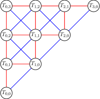
Fig. 2: Visualization of the triangle signal model. The $x_{1}$-shifts are blue colored and the $x_{2}$-shifts are red colored.

4 Christoffel-Darboux and the inverse transform

It would be quite nice if one has a unitary or orthogonal version of a discrete transform, since then one only needs to find and implement one algorithm for the computation of the transform and the computation of the inverse transform. It is well-known that in the case of 1D signal transforms the existence of unitary versions is connected to the basis polynomials of the signal module being orthogonal polynomials and relys on the Christoffel-Darboux formula for univariate orthogonal polynomials [9].

In the multivariate setting there is another constraint - the vanishing of all basis polynomials of the same degree. To see this, we recall the multivariate Christoffel-Darboux formula from [10]. Denote by $\mathbbm{T}_{k}=(T_{0,k},T_{1,k-1},\dots,T_{k,0})^{\top}$ the vector of bivariate Chebyshev polynomials of degree $k$. The vector $\mathbbm{T}_{k}$ is of length $k+1$. As the Chebyshev polynomials are orthogonal polynomials they satisfy three-term recurrence relations

$$x_{i}\mathbbm{T}_{k}=A_{k,i}\mathbbm{T}_{k+1}+B_{k,i}\mathbbm{T}_{k}+C_{k,i}\mathbbm{T}_{k-1},$$ (13)

were the matrices $A_{k,i},B_{k,i},$ and $C_{k,i}$ can be deduced from (9). For example from the $x_{1}$-shift one gets the matrices

$$\begin{split}A_{k,1}&=\begin{bmatrix}0&1/2&0&\dots&&0\\ 1/4&0&1/4&0&\dots&0\\ 0&\ddots&\ddots&\ddots&&\vdots\\ \dots&0&1/4&0&1/4&0\\ 0&\dots&0&1/2&0&1/4\end{bmatrix},\\ B_{k,1}&=\begin{bmatrix}0&\dots&&0\\ \vdots&\ddots&&\vdots\\ 0&\dots&0&0\\ 0&\dots&1/4&0\\ 0&\dots&0&0\end{bmatrix},C_{k,1}=\begin{bmatrix}0&1/2&0&\dots&0\\ 1/4&0&1/4&\ddots&\vdots\\ 0&\ddots&\ddots&\ddots&0\\ &&1/4&0&1/4\\ \vdots&&0&1/4&0\\ 0&\dots&&0&1/4\end{bmatrix},\end{split}$$ (14)

with special case $B_{1,1}=\begin{bmatrix}1/2&0\\ 0&0\end{bmatrix}$.

From the three-term recurrence relation one can deduce a multivariate Christoffel-Darboux formula [10]

$$\begin{split}&\sum_{k=0}^{n-1}\mathbbm{T}_{k}^{\top}(x)H_{k}^{-1}\mathbbm{T}_{k}(y)\\ &=\begin{cases}\begin{split}&(x_{i}-y_{i})^{-1}\cdot\\ &\big{(}(A_{n-1,i}\mathbbm{T}_{n}(x))^{\top}H_{n-1}^{-1}\mathbbm{T}_{n-1}(y)\\ &-\mathbbm{T}_{n-1}^{\top}(x)H_{n-1}^{-1}A_{n-1,i}\mathbbm{T}_{n}(y)\big{)}\end{split}&\text{if }x_{i}\not=y_{i}\\ \begin{split}&\mathbbm{T}_{n-1}^{\top}(x)H_{n-1}^{-1}A_{n-1,i}\tfrac{\partial}{\partial x_{i}}\mathbbm{T}_{n}(x)\\ &-(A_{n-1,i}\mathbbm{T}_{n}(x))^{\top}H_{n-1}^{-1}\tfrac{\partial}{\partial x_{1}}\mathbbm{T}_{n-1}(x)\end{split}&\text{if }x_{i}=y_{i},\end{cases}\end{split}$$ (15)

with matrices $H_{0}=\tfrac{1}{2}$ and $H_{k}=\mathsf{diag}(\tfrac{1}{8},\tfrac{1}{16},\dots,\tfrac{1}{16},\tfrac{1}{8})$.

Now one can observe that the entries of the matrix $\mathcal{F}_{n}^{\top}\cdot\mathcal{F}_{n}$ are of the form $\sum_{k=0}^{n-1}\mathbbm{T}_{k}^{\top}(\alpha)\mathbbm{T}_{k}(\beta)$ for $\alpha,\beta$ common zeros of $T_{n,0},T_{0,n}$. Thus consider the matrix $H_{n}^{\oplus}=\bigoplus_{k=0}^{n-1}H_{k}^{-1}$. Since the common zeros of $T_{n,0}$ and $T_{0,n}$ are in fact common zeros of all entries of $\mathbbm{T}_{n}$ one obtains the diagonal matrix

$$\mathcal{F}_{n}^{\top}\cdot H_{n}^{\oplus}\cdot\mathcal{F}_{n}=\mathsf{diag}\mathopen{}\mathclose{{}\left(\mathbbm{T}_{n-1}^{\top}(\alpha)H_{n-1}^{-1}A_{n-1,1}\tfrac{\partial}{\partial x_{1}}\mathbbm{T}_{n}(\alpha)}\right).$$ (16)

Since the diagonal entries of (16) do not vanish we can invert them. Denote the diagonal matrix with inverted entries by

$$D_{n}=\mathsf{diag}\mathopen{}\mathclose{{}\left(\mathopen{}\mathclose{{}\left(\mathbbm{T}_{n-1}^{\top}(x)H_{n-1}^{-1}A_{n-1,1}\tfrac{\partial}{\partial x_{1}}\mathbbm{T}_{n}(x)}\right)^{-1}}\right).$$ (17)

One obtains

$$\mathcal{F}_{n}^{-1}=D_{n}\mathcal{F}_{n}^{\top}H_{n}^{\oplus},$$ (18)

and in turn an orthogonal version of the triangle transform

$$\mathcal{F}_{n}^{\mathsf{orth}}=\sqrt{H_{n}^{\oplus}}\mathcal{F}_{n}\sqrt{D_{n}}.$$ (19)

5 Conclusions and future work

We developed a novel cosine transform on triangles and derived an orthogonal version of it. This showed the significance of multivariate Chebyshev polynomials and the multivariate Christoffel-Darboux formula for the derivation of orthogonal transforms.

To make the usage of these transforms applicable in real world applications a fast algorithm is essential. Since the multivariate Chebyshev polynomials obey a decomposition property (10), a fast algorithm exists. The implementation of this fast algorithm is currently under consideration and will be subject of upcoming work.

References

- [1] M. Bodner, J. Patera, and M. Szajewska, “Decomposition matrices for the special case of data on the triangular lattice of ,” Appl. Comput. Harmon. Anal., vol. 43, no. 2, pp. 346–353, 2017.
- [2] B. N. Ryland and H. Munthe-Kaas, “On multivariate Chebyshev polynomials and spectral approximations on triangles,” in Spectral and High Order Methods for Partial Differential Equations, J. S. Hesthaven and E. M. Ronquist, Eds., pp. 19–41. Springer, 2011.
- [3] M. Püschel and J.M.F. Moura, “Algebraic signal processing theory: Foundation and 1-D time,” Signal Processing, IEEE Trans., vol. 56, no. 8, pp. 3572–3585, 2008.
- [4] M. Püschel and J.M.F. Moura, “Algebraic signal processing theory: 1-D space,” Signal Processing, IEEE Trans., vol. 56, no. 8, pp. 3586–3599, 2008.
- [5] B. Seifert, K. Hüper, and C. Uhl, “Fast cosine transform for FCC lattices,” in Proc. of the 13th APCA International Conference on Automatic Control and Soft Computing, 2018, to appear.
- [6] M. Püschel and M. Rötteler, “Algebraic signal processing theory: 2-D spatial hexagonal lattice,” IEEE Trans. Image Process., vol. 16, no. 6, pp. 1506–1521, 2007.
- [7] M. E. Hoffman and W. D. Withers, “Generalized Chebyshev polynomials associated with affine Weyl groups,” Trans. Amer. Math. Soc., vol. 308, pp. 91–104, 1988.
- [8] J.H. Conway and N.J.A. Sloane, Sphere Packings, Lattices and Groups, Springer, third edition, 1999.
- [9] Y. Yemini and J. Pearl, “Asymptotic properties of discrete unitary transforms,” IEEE Trans. on Pattern Analysis and Machine Intelligence, vol. PAMI-1, no. 4, pp. 366–371, 1979.
- [10] Y. Xu, “On multivariable orthogonal polynomials,” SIAM J. Math. Anal., vol. 24, pp. 783–794, 1993.
- [11] M. Püschel and J.M.F. Moura, “Algebraic signal processing theory: Cooley-Tukey type algorithms for DCTs and DSTs,” Signal Processing, IEEE Trans., vol. 56, no. 4, pp. 1502–1521, 2008.