The control set of a linear control system on the two dimensional solvable Lie group

Abstract

In this paper we explicitly calculate the control sets associated with a linear control system on the two dimensional solvable Lie group. We show that a linear control system of such kind admits exactly one control set or infinite control sets depending on some algebraic conditions.

Keywords: linear control systems, solvable Lie group

Mathematics Subject Classification (2010): 93B05, 93C05, 22E25

1 Introduction

The classical linear control systems on Euclidean Spaces are well known. They are relevant for many theoretical and practical reasons. In particular, they appear in several physical applications ([12, 14, 15]). They are naturally extended to general Lie groups as showed in [13] for matrices groups, and then in [4] for any connected Lie group $G$.

In the last twenty-five years, several works addressing controllability, observability and optimization problems appears for this kind of control systems, (see [1, 2, 3, 7, 8, 9, 10]). Furthermore, in [10] Jouan shows that any affine control system on a connected manifold that generates a finite dimensional Lie algebra is diffeomorphic to a linear control system on a Lie group, or on a homogeneous space. Hence, such kind of generalization is also relevant for the classification of general affine control systems on abstract connected manifolds.

A fundamental notion in control theory is the controllability property of a control system answering the following question: given an initial state of the system, is it possible to reach any arbitrary state through admissible trajectories in positive time? Or better, there are some regions of the space of state where controllability holds? For instance, in [11] the authors work out the problem Optimal controls for a two-compartment model for cancer chemotherapy  with quadratic objective. The space state of this model is the plane, and its dynamic is given by two matrices which are elements of the Lie algebra $\mathrm{sl}(2,\mathbb{R})$, of real matrices of order two and trace zero, see [5] for an algebraic controllability condition. Therefore, in this case, the controllability property reads as: given an initial condition $x_{0}$ there exists an admissible control transferring $x_{0}$ in positive time in a new condition $x_{1}.$ In other words, is it possible to find a medical strategy to transform an initial level of disease, at another final level of health, in a positive time$?$. Among the all possibles estrategies transfering $x_{0}$ into $x_{1}$, you need to find the optimal control which minimizes the quadratic objective. In our practical example, to find the optimal control which minimizes the collateral effects.

In real life, not any sick condition can be transformed in a health one. Since in the interior $\mathrm{int}(\mathcal{C)}$ of any control set $\mathcal{C}$ controllability holds, it is fundamental to know about the existence and uniqueness of control sets, especially those with non empty interior. And certainly, to characterize the control sets of a control system in any possible case. The main goal of this paper is to compute every control set for a linear control system on a solvable Lie group of dimension two, with and without empty interior.

Because of our intention to reach an audience as bigger as possible, we avoid describing a linear control system as usual through the Lie theory. On the contrary, we look at linear control systems as special systems evolving on an open half-plane of $\mathbb{R}^{2}$. Furthermore, aiming a better understanding and reading of the article, we have include figures of each possible control set.

The paper is structured as follows: Section 2 contains the basic definition of control systems, accessible and control sets. We also describe the two dimensional solvable Lie groups given by the open half-plane $G=\mathbb{R}_{+}\times\mathbb{R}$ endowed with its associated non Abelian product.  In section 3 we describe case by case the control sets of linear control systems that are conjugated with our initial system. That allow us to know when such sets have empty or nonempty interior and their uniqueness. Finally, at the end of Section 3 we use the group of automorphisms of $G$ in order to see what are the possibilities for the control sets of a general linear control system on $G$.

2 Preliminaries

2.1 Control systems and their control sets

Let $M$ be a $d$-dimensional smooth manifold. A control system in $M$ is the family of ordinary differential equations

$$\dot{x}(t)=f(x(t),u(t)),\;\;\;u\in\mathcal{U},$$

where $f:M\times\mathbb{R}^{m}\rightarrow TM$ is a smooth map and $\mathcal{U}\subset L_{\mathrm{loc}}^{\infty}(\mathbb{R},\mathbb{R}^{m})$ is the set of the piecewise constant functions whose image are contained in a compact convex set $\Omega\subset\mathbb{R}^{m}$. For any $x\in M$ and $u\in\mathcal{U}$ we denote by $\phi(t,x,u)$ the unique solution of (2.1) with initial value $x=\varphi(0,x,u)$. The set of points reachable from $x$ up to time $\tau>0$ and the positive orbit of $x$ are given, respectively, by

$$\mathcal{O}^{+}_{\leq\tau}(x):=\{\varphi(t,x,u),\;\;t\in[0,\tau]\;\;u\in\mathcal{U}\}\;\;\;\mbox{ and }\;\;\;\mathcal{O}^{+}(x):=\bigcup_{t>0}\mathcal{O}^{+}_{t}(x).$$

With $\mathcal{O}^{-}_{\leq\tau}(x)$ and $\mathcal{O}^{-}(x)$ we denote the corresponding sets for the time-reversed system. We say that the system (2.1) is locally accessible from $x$ if $\mathrm{int}\mathcal{O}^{\pm}_{\leq\tau}(x)\neq\emptyset$ for all $\tau>0$. A sufficiente condition for locally accessibility is the Lie algebra rank condition (LARC). It is satisfied if the Lie algebra $\mathcal{L}$ generated by the vector fields $x\in M\mapsto f_{u}(x):=f(x,u)$, for $u\in\Omega$, satisfies $\mathcal{L}(x)=T_{x}M$ for all $x\in M$.

A set $\mathcal{C}\subset M$ is a control set of 2.1 if it is maximal w.r.t. set inclusion with the following properties:

1. $\mathcal{C}$ is controlled invariant, i.e., for each $x\in\mathcal{C}$ there is $u\in\mathcal{U}$ with $\varphi(\mathbb{R}_{+},x,u)\subset\mathcal{C}$.

2. Approximate controllability holds on $\mathcal{C}$, i.e., $\mathcal{C}\subset\operatorname{cl}\mathcal{O}^{+}(x)$ for all $x\in\mathcal{C}$.

Following [6], Proposition 3.2.4., any subset $\mathcal{C}$ of $M$ with nonempty interior that is maximal with property (ii) in the above definition is a control set.

Let us consider $\psi:M\rightarrow N$ to be a diffeomorphism and consider

$$\dot{x}(t)=f(x(t),u(t))\;\;\mbox{ and }\;\;\dot{y}(t)=g(y(t),u(t))\;\;\;u\in\mathcal{U}$$

control systems on $M$ and $N$, respectively. We say that $\psi$ conjugates the control systems if

$$g(\psi(x),u)=(d\psi)_{x}f(x,u)\;\;\mbox{ for any }\;\;x\in G,u\in\mathcal{U}.$$

In this cases we say that the control systems are equivalent. The conjugation of control systems will be used ahead several times.

2.2 Two-dimensional linear control systems

In this section we analyze linear control systems on the two-dimensional solvable Lie group.

Let us denote by $G=\mathbb{R}_{+}\times\mathbb{R}$ the open half-plane of $\mathbb{R}^{2}$ and endow it with the product

$$(x_{1},y_{1})\cdot(x_{2},y_{2})=(x_{1}x_{2},y_{2}+x_{2}y_{1}).$$

It is a standard fact that the $G$ is in fact a Lie group and, up to an isomorphism, is the unique two-dimensional solvable Lie group.

Following [8], a linear vector field on $G$ is a vector field of the form

$$\mathcal{X}(x,y)=(0,a(x-1)+by),\;\;\mbox{ for some }\;\;(a,b)\in\mathbb{R}^{2}.$$

Moreover, a simple calculation shows that the left-invariant vector fields of $G$ are of the form

$$Y(x,y)=(x\alpha,x\beta),\;\;\mbox{ for some }\;\;(\alpha,\beta)\in\mathbb{R}^{2}.$$

Let $\Omega=[u_{*},u^{*}]$ with $u_{*}<0<u^{*}$. A linear control system on $G$ is a system of the form

$$\dot{(x,y)}=\mathcal{X}(x,y)+uY(x,y),\;\;\;\mbox{ with }\;\;u\in\Omega,$$

where $\mathcal{X}$ and $Y$ are nontrivial vector fields. In coordinates,

$$(\Sigma)\hskip 56.9055pt\left\{\begin{array}[c]{l}\dot{x}=u\alpha x\\ \dot{y}=a(x-1)+by+ux\beta\end{array}\right.,\;\;\mbox{ where }\;\;u\in\Omega\;\;\mbox{ and }\;\;(a,b),(\alpha,\beta)\in\mathbb{R}^{2}\setminus\{(0,0)\}.$$

A simple calculation shows that

$$\mathcal{L}(x,y)=\mathrm{span}\{(u\alpha x,a(x-1)+by+ux\beta),(0,ux(a\alpha+b\beta)),\;\;u\in\Omega\}$$

and $\mathcal{L}(x,y)=\mathbb{R}^{2}$ for all $(x,y)\in G$ if and only if $\alpha(a\alpha+b\beta)\neq 0$, that is, the LARC holds for $\Sigma$ if and only if $\alpha(a\alpha+b\beta)\neq 0$.

In order to analyze the control sets of $\Sigma$ it will be necessary to conjugate the system in order to simplify it. Because of that we need the following notion: An automorphism of $G$ is a map $\psi:G\rightarrow G$ that preserves the product, that is,

$$\psi((x_{1},y_{1})\cdot(x_{2},y_{2}))=\psi(x_{1},y_{1})\cdot\psi(x_{2},y_{2}),\;\;(x_{1},y_{1}),(x_{2},y_{2})\in G.$$

The automorphisms $\psi:G\rightarrow G$ have the form

$$\psi(x,y)=(x,c(x-1)+dy),\;\;d\in\mathbb{R}^{\ast}.$$

Moreover, the automorphisms of $G$ preserves linear and left-invariant vector fields and hence conjugates linear control systems. This fact will be used ahead several times in order to simplify calculations.

3 The control sets of linear control systems on $G$

The aim of this section, is analyze the control sets of a given linear control system. In order to do that we conjugate the given system by an automorphism in to simplify the calculations and make the problem more abordable to deal with.

The next result, which we will prove through the following sections summarize our findings.

3.1 Theorem:

For the control system $\Sigma$ it holds that

• If $\alpha=0$ then $\Sigma$ has infinite control sets;

• If $\alpha\neq 0$ then $\Sigma$ admits a unique control set that has nonempty interior if and only if the LARC holds.

The proof of the theorem is divided in the next sections.

3.1 The case $\alpha=a\alpha+b\beta=0$

Since $(a,b),(\alpha,\beta)\in\mathbb{R}^{2}\setminus\{(0,0)\}$ the above condition implies that $\alpha=b=0$ and $a,\beta\in\mathbb{R}^{\ast}$ and therefore, the system $\Sigma$ is of the form,

$$\left\{\begin{array}[c]{l}\dot{x}=0\\ \dot{y}=a(x-1)+ux\beta\end{array}\right.,\;\;\mbox{ where }\;\;u\in\Omega,$$

whose solutions starting at $(x,y)\in G$ are given by

$$\varphi(t,(x,y),u)=(x,(a(x-1)+ux\beta)t+y),\;\;t\in\mathbb{R}.$$

We claim

$$\mathcal{C}_{x}:=\{x\}\times\mathbb{R}\;\mbox{ is a control set for any }\;x\in(1-\varepsilon,1+\varepsilon).$$

In fact, for any $x\in\mathbb{R}_{+}$ the line $\{x\}\times\mathbb{R}\subset G$ is invariant by the solutions of $\Sigma$. On the other hand, if $x\in(1-\varepsilon,1+\varepsilon)$ and there exist $u_{1},u_{2}\in\Omega$ such that $a(x-1)+u_{1}x\beta<0$ and $a(x-1)+u_{2}x\beta>0$. Hence, it turns out that

$$\varphi_{2}(t,(x,y),u_{1})\rightarrow-\infty\;\;\mbox{ and }\;\;\varphi_{2}(t,(x,y),u_{2})\rightarrow+\infty\;\mbox{ as }\;t\rightarrow+\infty$$

where $\varphi_{2}$ stands for the second component of $\varphi$. Therefore, $\mathcal{O}^{+}(x,y)=\{x\}\times\mathbb{R}$ for any $y\in\mathbb{R}$ implying that $\mathcal{C}_{x}$ is a control set for any $x\in(1-\varepsilon,1+\varepsilon)$ (see Figure 1). In particular, the control system $\Sigma$ admits an infinite number of control sets.

Figure 1: The control sets of $\Sigma$.

3.2 The case $\alpha=0$ and $a\alpha+b\beta\neq 0$

In this case, we necessarily have that $b,\beta\in\mathbb{R}^{\ast}$. Therefore, the map $\psi(x,y):=(x,a(x-1)+by)$ is an automorphism of $G$ that conjugates $\Sigma$ and the linear control system,

$$\left\{\begin{array}[c]{l}\dot{x}=0\\ \dot{y}=by+uxb\beta\end{array}\right.,\;\;\mbox{ where }\;\;u\in\Omega,$$ (1)

whose solutions starting at $(x,y)\in G$ are given by

$$\varphi(t,(x,y),u)=(x,\mathrm{e}^{tb}y+(\mathrm{e}^{tb}-1)ux\beta),\;\;t\in\mathbb{R}.$$

Let us analyze the case where $b<0$ since the other case is analogous. For any given $x\in\mathbb{R}_{+}$ we use the compactness of $\Omega$ to define

$$y_{1}(x):=\min\{-ux\beta,\;\;u\in\Omega\}\;\;\mbox{ and }\;\;y_{2}(x):=\max\{-ux\beta,\;\;u\in\Omega\}.$$

Since $0\in\operatorname{int}\Omega$ we get $y_{1}(x)<0<y_{2}(x)$. We claim that the set

$$\mathcal{C}_{x}=\{x\}\times\left[y_{1}(x),y_{2}(x)\right]$$

is a positively-invariant control set of (1). In fact, for any $u\in\Omega$ and $y\in\left[y_{1}(x),y_{2}(x)\right]$ it holds that

$$y_{1}(x)-\varphi_{2}(t,(x,y),u)=y_{1}(x)-\mathrm{e}^{tb}y+(1-\mathrm{e}^{tb})ux\beta$$

$$\leq y_{1}(x)-\mathrm{e}^{tb}y_{1}(x)+(1-\mathrm{e}^{tb})ux\beta\leq(1-\mathrm{e}^{tb})(y_{1}(x)+ux\beta)\leq 0\implies y_{1}(x)\leq\varphi_{2}(t,(x,y),u)$$

and

$$y_{2}(x)-\varphi_{2}(t,(x,y),u)=y_{2}(x)-\mathrm{e}^{bt}y+(1-\mathrm{e}^{tb})ux\beta$$

$$\geq y_{2}(x)-\mathrm{e}^{bt}y_{2}(x)+(1-\mathrm{e}^{tb})ux\beta=(1-\mathrm{e}^{bt})(y_{2}(x)+ux\beta)\geq 0\implies\varphi_{2}(t,(x,y),u)\leq y_{2}(x)$$

showing that $\mathcal{C}_{x}$ is positively-invariant.

Let $u_{1},u_{2}\in\Omega$ such that $y_{i}(x)+u_{i}x\beta=0,\;i=1,2$. Then, for any $y\in(y_{1}(x),y_{2}(x))$ we have that

$$\varphi_{2}(t,(x,y),u_{i})\rightarrow-u_{i}x\beta=y_{i}(x)$$

implying that $\mathcal{C}_{x}\subset\operatorname{cl}\mathcal{O}^{+}(x,y)$ for any $y\in(y_{1}(x),y_{2}(x))$. By continuity and invariance, we get that

$$\mathcal{C}_{x}=\operatorname{cl}\mathcal{O}^{+}(x,y),\;\;\mbox{ for any }\;\;(x,y)\in\mathcal{C}_{x}$$

concluding the proof.

A simple calculation shows that $[y_{1}(x_{0}),y_{2}(x_{0})]\subset[y_{1}(x_{1}),y_{2}(x_{1})]$ if $x_{0}<x_{1}$. Hence (1) admits an infinite number of control sets (see Figure 2).

Figure 2: The control sets of (1).

3.3 The case $\alpha\neq 0$ and $a\alpha+b\beta=0$

In this case, we necessarily have that $b\neq 0$. Let us consider the automorphis of $G$ given by $\psi(x,y):=(x,y-(x-1)\beta\alpha^{-1})$. We have that $\psi$ conjugates $\Sigma$ and the linear control system

$$\left\{\begin{array}[c]{l}\dot{x}=u\alpha x\\ \dot{y}=by\end{array}\right.,\;\;\mbox{ where }\;\;u\in\Omega,$$ (2)

whose solutions starting at $(x,y)\in G$ are given by concatenations of flows

$$\varphi(t,(x,y),u)=(\mathrm{e}^{tu\alpha}x,\mathrm{e}^{tb}y),\;\;t\in\mathbb{R}.$$

For the above control system, the only control set is given by $\mathcal{C}=\mathbb{R}_{+}\times\{0\}$.

Let us first show that $\mathcal{C}$ is a control set. We notice that $\varphi(t,\mathcal{C},u)\subset\mathcal{C}$ for any $u\in\Omega$ and $t\in\mathbb{R}$. On the other hand, if $\varphi_{1}$ is the first component of $\varphi$, it holds that

$$\left\{\begin{array}[c]{l}\varphi_{1}(t,(x,0),u)\rightarrow+\infty,\;\;\mbox{ for }\;\;t\rightarrow+\infty\;\;\mbox{ when }\;\;\alpha u>0\\ \varphi_{1}(t,(x,0),u)\rightarrow 0,\;\;\;\;\mbox{ for }\;\;t\rightarrow+\infty\;\;\mbox{ when }\;\;\alpha u<0\end{array}\right.,$$

implying that $\mathcal{C}=\operatorname{cl}(\mathcal{O}^{+}(x,0))$ for any $x\in\mathbb{R}_{+}$ and consequently that $\mathcal{C}$ is a control set.

Let us assume that $b<0$ and show the uniqueness. The case $b>0$ is analogous. In order to do it is enough to show that no point in $G$ outside $\mathcal{C}$ satisfies condition (ii) in the definition of control sets.

In fact, let $(x_{0},y_{0})\in G$ with $y_{0}\neq 0$. By the form of the solutions $\operatorname{cl}(\mathcal{O}^{+}(x_{0},y_{0}))$ is comprehended between the lines $y=0$ and $y=y_{0}$. Moreover, if $(x_{1},y_{1})\in\mathcal{O}^{+}(x_{0},y_{0})$ there exists $t_{0}>0$ such that $y_{1}=\mathrm{e}^{bt_{0}}y_{0}<y_{0}$ if $y_{0}>0$ and $y_{1}=\mathrm{e}^{bt_{0}}y_{0}>y_{0}$ if $y_{0}<0$. Thus $(x_{0},y_{0})$ is outside the region determine by the lines $y=0$ and $y=y_{1}$ and therefore $(x_{0},y_{0})\notin\operatorname{cl}(\mathcal{O}^{+}(x_{1},y_{1}))$ if $(x_{1},y_{1})\in\operatorname{cl}(\mathcal{O}^{+}(x_{0},y_{0}))$. Consequently, no points in $\mathcal{M}\setminus\mathcal{C}$ can be inside a control set implying the uniqueness of $\mathcal{C}$ (see Figure 3).

Figure 3: The control set $\mathcal{C}$ of (2) and the behavior of the solutions outside $\mathcal{C}$.

3.4 The case $\alpha(a\alpha+b\beta)\neq 0$

In this section, we analyze the control sets under the LARC. As Theorem 3.1 states in this case we have the associated control set is unique and has nonempty interior. We will divide the analysis in the following two sections.

3.4.1 The case $b=0$

In this situation, we necessarily have that $a\neq 0$ and so $\psi(x,y):=(x,a^{-1}y-\beta\alpha^{-1}(x-1))$ is a diffeomorphism that conjugates $\Sigma$ and the control system

$$\left\{\begin{array}[c]{l}\dot{x}=u\alpha x\\ \dot{y}=x-1\end{array}\right.,\;\;\mbox{ where }\;\;u\in\Omega,$$ (3)

whose solutions starting at $(x,y)\in G$ are given by concatenations of the flows

$$\varphi(t,(x,y),u)=\left(\mathrm{e}^{u\alpha t}x,\frac{(\mathrm{e}^{u\alpha t}-1)x}{u\alpha}-t+y\right),\;\;t\in\mathbb{R},\;\;u\neq 0$$

and

$$\varphi(t,(x,y),0)=\left(x,(x-1)t+y\right),\;\;t\in\mathbb{R},\;\;u=0.$$

Before showing that the control system (3) is controllable it is important to notice that in [8] the authors prove that $b=0$ and the LARC are equivalent to the controllability of a linear control system. The difference here is that we show explicitly “the way´´such controllability is obtained. This is certainly worth since one can use it in optimability problems concerning such systems.

Let then $(x_{1},y_{1}),(x_{2},y_{2})\in G$ and assume that $x_{1}<1<x_{2}$. It holds:

• $(x_{2},y_{2})\in\mathcal{O}^{+}(x_{1},y_{1}):$

  In fact, let $u\in\Omega$ with $u\alpha>0$. Since $\varphi_{1}(t,(x_{1},y_{1}),u)=\mathrm{e}^{u\alpha t}x_{1}$ there exists $t_{1}>0$ such that $\varphi_{1}(t_{1},(x_{1},y_{1}),u)=x_{2}$. By considering $y_{2}^{\prime}:=\varphi_{2}(t_{1},(x_{1},y_{1}),u)$ we have that:

  • Assume $y_{2}^{\prime}\leq y_{2}$. Since $x_{2}>1$ it follows that $t_{2}:=\frac{y_{2}-y_{2}^{\prime}}{x_{2}-1}\geq 0$. Consequently

    $$\varphi(t_{2},(x_{2},y_{2}^{\prime}),0)=(x_{2},(x_{2}-1)t_{2}+y_{2}^{\prime})=(x_{2},y_{2})\;\;\implies\varphi(t_{2},\varphi(t_{1},(x_{1},y_{1}),u),0)=(x_{2},y_{2}).$$

    Therefore $(x_{2},y_{2})\in\mathcal{O}^{+}(x_{1},y_{1})$;

  • Assume $y_{2}^{\prime}>y_{2}$. Since $y\mapsto\frac{(\mathrm{e}^{u\alpha t_{1}}-1)x_{1}}{u\alpha}-t_{1}+y$ is strictly increasing, there exists $y_{1}^{\prime}<y_{1}$ such that

    $$\varphi_{2}(t_{1},(x_{1},y_{1}^{\prime}),u)=\frac{(\mathrm{e}^{u\alpha t_{1}}-1)x_{0}}{u\alpha}-t_{1}+y_{1}^{\prime}=y_{2}.$$

    Since $x_{1}<1$ we have that $t_{0}=\frac{y_{1}^{\prime}-y_{1}}{x_{1}-1}>0$ and hence

    $$\varphi(t_{0},(x_{1},y_{1}),0)=(x_{1},(x_{1}-1)t_{0}+y_{1})=(x_{1},y_{1}^{\prime})\;\;\implies\;\;\varphi(t_{1},\varphi(t_{0},(x_{1},y_{1}),u),0)=(x_{2},y_{2})$$

    implying that $(x_{2},y_{2})\in\mathcal{O}^{+}(x_{1},y_{1})$ (see Figure 4).

  
  

• $(x_{1},y_{1})\in\mathcal{O}^{+}(x_{2},y_{2}):$

  Let $u\in\Omega$ with $u\alpha<0$. Since $\varphi_{1}(t,(x_{2},y_{2}),u)=\mathrm{e}^{u\alpha t}x$ there exists $t_{1}>0$ such that $\varphi_{1}(t_{1},(x_{2},y_{2}),u)=x_{1}$. By considering $y_{1}^{\prime}:=\varphi_{2}(t_{1},(x_{2},y_{2}),u)$ we have that:

  • Assume $y_{1}^{\prime}\geq y_{1}$. Since $x_{1}<1$ it follows that $t_{2}:=\frac{y_{1}-y_{1}^{\prime}}{x_{1}-1}\geq 0$. Consequently

    $$\varphi(t_{2},(x_{1},y_{1}^{\prime}),0)=(x_{1},(x_{1}-1)t_{2}+y_{1}^{\prime})=(x_{1}y_{1})\;\;\implies\varphi(t_{2},\varphi(t_{1},(x_{2},y_{2}),u),0)=(x_{1},y_{1}).$$

    Therefore $(x_{1},y_{1})\in\mathcal{O}^{+}(x_{2},y_{2})$;

  • Assume $y_{1}^{\prime}<y_{1}$. Since $y\mapsto\frac{(\mathrm{e}^{u\alpha t_{1}}-1)x_{2}}{u\alpha}-t_{1}+y$ is strictly increasing, there exists $y_{2}^{\prime}>y_{2}$ such that

    $$\varphi_{2}(t_{0},(x_{2},y_{2}^{\prime}),u)=\frac{(\mathrm{e}^{u\alpha t}-1)x_{2}}{u\alpha}-t+y_{2}^{\prime}=y_{1}.$$

    Since $x_{2}>1$ we have that $t_{0}=\frac{y_{2}^{\prime}-y_{2}}{x_{2}-1}>0$ and hence

    $$\varphi(t_{0},(x_{2},y_{2}),0)=(x_{2},(x_{2}-1)t_{0}+y_{2})=(x_{2},y_{2}^{\prime})\;\;\implies\;\;\varphi(t_{1},\varphi(t_{0},(x_{2},y_{2}),0),u)=(x_{1},y_{1})$$

    implying that $(x_{1},y_{1})\in\mathcal{O}^{+}(x_{2},y_{2}).$

Figure 4: Solutions of (2) connecting distinct points.

Now we are able to prove a controllability result.

3.2 Theorem:

If $b=0$ the only control set of $\Sigma$ is the whole space $G$.

Proof.

By conjugation it is enough to show that $G$ is the control set of the control system (3). Let us consider $(x_{1},y_{1}),(x_{2},y_{2})\in G\setminus\{(1,y),y\in\mathbb{R}\}$. If $x_{1}>1$ and $x_{2}>1$ we can consider $u\in\Omega$ with $u\alpha<0$ and, since $\mathrm{e}^{u\alpha t}x_{1}\rightarrow 0$ as $t\rightarrow+\infty$ there exists $t_{0}>0$ such that $x_{1}^{\prime}=\mathrm{e}^{u\alpha t_{0}}x_{1}<1$. By the above, it holds that $(x_{2},y_{2})\in\mathcal{O}^{+}(\varphi(t_{0},(x_{1},y_{1}),u))$ and hence $(x_{2},y_{2})\in\mathcal{O}^{+}(x_{1},y_{1})$. An analogous analysis for the case $x_{1}<1$ and $x_{2}<1$ gives us also $(x_{2},y_{2})\in\mathcal{O}^{+}(x_{1},y_{1})$ and consequently

$$G\setminus\{(1,y),y\in\mathbb{R}\}\subset\mathcal{O}^{+}(x,y),\;\;\mbox{ for any }\;\;(x,y)\in G\setminus\{(1,y),y\in\mathbb{R}\}.$$

Since $G\setminus\{(1,y),y\in\mathbb{R}\}$ is certainly dense in $G$ we get that $G\subset\operatorname{cl}(\mathcal{O}^{+}(x,y))$ for any $(x,y)\in G\setminus\{(1,y),y\in\mathbb{R}\}$. On the other hand, for any $(x,y)\in G$ there exists $u\in\Omega$ and $t>0$ such that $\varphi(t,(x,y),u)\in G\setminus\{(1,y),y\in\mathbb{R}\}$. Finally,

$$G\subset\operatorname{cl}(\mathcal{O}^{+}(\varphi(t,(x,y),u)))\subset\operatorname{cl}(\mathcal{O}^{+}(x,y))\subset G$$

implying that $G$ is the only control set of (3) and concluding the proof. ∎

3.4.2 The case $b\neq 0$

Since the sign of $b$ in not relevant for the proof, we only consider the case $b<0$. By considering the diffeomorphism of $G$ defined by $\psi(x,y):=(x,\gamma^{-1}(a(x-1)+by))$, where $\gamma=a\alpha+b\beta\neq 0$, it follows that $\Sigma$ is conjugated to the control system

$$\left\{\begin{array}[c]{l}\dot{x}=u\alpha x\\ \dot{y}=by+ux\end{array}\right.,\;\;\mbox{ where }\;\;u\in\Omega.$$ (4)

The solutions starting at $(x,y)\in G$ of (4) are given by concatenations of the flows

$$\begin{array}[c]{c}\varphi(t,(x,y),u)=(\mathrm{e}^{u\alpha t}x,m_{u}(\mathrm{e}^{u\alpha t}-\mathrm{e}^{bt})x+\mathrm{e}^{bt}y),\;\;\mbox{ for }u\alpha\neq b\;\;\mbox{ and }\;\;m_{u}=\frac{u}{u\alpha-b}\\ \\ \mbox{ and }\;\;\;\varphi(t,(x,y),b\alpha^{-1})=\left(\mathrm{e}^{bt}x,\mathrm{e}^{tb}(y+tb\alpha^{-1}x)\right),\;\;t\in\mathbb{R},\;\;\mbox{ when }\;u\alpha=b.\end{array}$$ (5)

For any $u\in\Omega$ with $u\alpha\neq b$ we denote by $r_{u}$ the ray of $G$ given by

$$r_{u}:=\{(x,y)\in G;\;\;y-m_{u}x=0\},$$

that is, $r_{u}$ is the intersection with $G$ of the line by the origin of $\mathbb{R}^{2}$ with inclination $m_{u}$.

Define $m:\mathbb{R}\setminus\{b\alpha^{-1}\}\rightarrow\mathbb{R}$ to be the map given by $u\mapsto m_{u}$. It is straightforward to see that (see Figure 5)

• $m_{u}=\frac{-b}{(u\alpha-b)^{2}}>0$ and so, $m$ is strictly increasing on $(-\infty,b\alpha^{-1})$ and on $(b\alpha^{-1},+\infty)$;

• $\lim_{u\rightarrow\pm\infty}m_{u}=\alpha^{-1}$ and $\lim_{u\rightarrow(b\alpha^{-1})^{\pm}}m_{u}=\mp\infty$.

Figure 5: Behavior of $m_{u}$.

Let us consider $B:=\{u\in\Omega;\;u\alpha-b>0\}$. Since we are assuming $b<0$ and $0\in\mathrm{int}\Omega$ we necessarily have that $u\alpha-b>0$ for some $u\in\Omega$ and consequently $B\neq\emptyset$. For the solutions of the above control system we have the following:

3.3 Proposition:

For any $t>0$ and $u\in\Omega$ it holds:

• $\varphi_{t,u}(r_{u})\subset r_{u}$;

• $\varphi(t,(x,y_{1}+y_{2}),u)=\varphi(t,(x,y_{1}),u)+(0,\mathrm{e}^{bt}y_{2})$;

• For $u\alpha\neq 0$ we obtain

  $$m_{u_{*}}\varphi_{1}(t,(x,y),u)-\varphi_{2}(t,(x,y),u)\leq\mathrm{e}^{bt}(m_{u_{*}}x-y)\;\;\mbox{ if }\;\;u_{*}\in B;$$

  $$\varphi_{1}(t,(x,y),u)-m_{u^{*}}\varphi_{1}(t,(x,y),u)\leq\mathrm{e}^{bt}(y-m_{u^{*}}x)\;\;\mbox{ if }\;\;u^{*}\in B.$$

• For $u=b\alpha^{-1}$ we get

  $$m_{u_{*}}\varphi_{1}(t,(x,y),u)-\varphi_{2}(t,(x,y),u)\leq\mathrm{e}^{bt}(m_{u_{*}}x-y)\;\;\mbox{ if }\;\;\alpha<0,\;\;\mbox{ and }\;\;$$

  $$\varphi_{1}(t,(x,y),u)-m_{u^{*}}\varphi_{1}(t,(x,y),u)\leq\mathrm{e}^{bt}(y-m_{u^{*}}x)\;\;\mbox{ if }\;\;\alpha>0.$$

Proof.

Since a general solution of (4) is given by concatenations of the flows in (5) it is enough to show the proposition for $u\in\Omega$.

1. In fact, if $(x,y)\in r_{u}$ we have that $y=m_{u}x$ and for any $(x,y)\in r_{u}$

$$\varphi(t,(x,y),u)=(\mathrm{e}^{\alpha ut}x,m_{u}(\mathrm{e}^{u\alpha t}-\mathrm{e}^{bt})x+\mathrm{e}^{bt}m_{u}x)=(\mathrm{e}^{\alpha ut}x,\mathrm{e}^{\alpha ut}m_{u}x)=\mathrm{e}^{\alpha ut}(x,y).$$

2. In fact, if $u\alpha\neq b$ we get

$$\varphi(t,(x,y_{1}+y_{2}),u)=(\mathrm{e}^{u\alpha t}x,m_{u}(\mathrm{e}^{u\alpha t}-\mathrm{e}^{bt})x+\mathrm{e}^{bt}(y_{1}+y_{2}))$$

$$=(\mathrm{e}^{u\alpha t}x,m_{u}(\mathrm{e}^{u\alpha t}-\mathrm{e}^{bt})x+\mathrm{e}^{bt}y_{1})+(0,\mathrm{e}^{bt}y_{2})=\varphi(t,(x,y_{1}),u)+(0,\mathrm{e}^{bt}y_{2})$$

and for $u\alpha=b$

$$\varphi(t,(x,y_{1}+y_{2}),b\alpha^{-1})=\left(\mathrm{e}^{bt}x,\mathrm{e}^{tb}(y_{1}+y_{2}+tb\alpha^{-1}x)\right)$$

$$\left(\mathrm{e}^{bt}x,\mathrm{e}^{tb}(y_{1}+tb\alpha^{-1}x)\right)+(0,\mathrm{e}^{tb}y_{2})=\varphi(t,(x,y_{1}),b\alpha^{-1})+(0,\mathrm{e}^{bt}y_{2}).$$

3. Let us analyze the case for $u_{*}\in B$. We have that

$$m_{u_{*}}\varphi_{1}(t,(x,y),u)-\varphi_{2}(t,(x,y),u)=m_{u_{*}}\mathrm{e}^{u\alpha t}x-m_{u}\mathrm{e}^{u\alpha t}x+m_{u}\mathrm{e}^{bt}x-\mathrm{e}^{bt}y=(m_{u_{*}}-m_{u})\mathrm{e}^{u\alpha t}x+\mathrm{e}^{bt}x-\mathrm{e}^{bt}y$$

However, if $u\alpha-b>0$ then $m_{u_{*}}\leq m_{u}$ implying that $(m_{u_{*}}-m_{u})\mathrm{e}^{u\alpha t}\leq(m_{u_{*}}-m_{u})\mathrm{e}^{bt}$. If $u\alpha-b<0$ then $m_{u_{*}}>m_{u}$ and consequently $(m_{u_{*}}-m_{u})\mathrm{e}^{u\alpha t}\leq(m_{u_{*}}-m_{u})\mathrm{e}^{bt}$. Therefore,

$$m_{u_{*}}\varphi_{1}(t,(x,y),u)-\varphi_{2}(t,(x,y),u)\leq(m_{u_{*}}-m_{u})\mathrm{e}^{bt}+m_{u}\mathrm{e}^{bt}x-\mathrm{e}^{bt}y=\mathrm{e}^{bt}(m_{u_{*}}x-y),\;\;u\alpha-b\neq 0.$$

4. If $\alpha<0$ we obtain $b\alpha^{-1}>0$ and hence

$$m_{u_{*}}\varphi_{1}(t,(x,y),b\alpha^{-1})-\varphi_{2}(t,(x,y),b\alpha^{-1})=m_{u_{*}}\mathrm{e}^{bt}x-\mathrm{e}^{bt}(y+tb\alpha^{-1}x)\leq\mathrm{e}^{bt}(m_{u_{*}}x-y).$$

∎

3.4 Remark:

By concatenations, itens 2 to 4 are also valid for any piecewise constant function $u\in\mathcal{U}$.

Let us consider the set

$$\mathcal{C}:=\bigcup_{u\in B}r_{u}.$$

Our aim is to show that $\mathcal{C}$ is in fact the only control set of (4). In order to that the next lemma, concerning the main properties of $\mathcal{C}$, will be central.

3.5 Lemma:

Let $u\in\Omega$. It holds:

• If $b\notin\alpha\Omega$, then

  $$\mathcal{C}=\{(x,y)\in G;\;\;m_{u_{*}}x\leq y\leq m_{u^{*}}x\};$$

• If $b\in\alpha\Omega$, then

  $$\mathcal{C}=\{(x,y)\in G;\;\;y\leq m_{u^{*}}x\}\;\;\mbox{ if }\;\;\alpha>0\;\;\mbox{ and }$$

  $$\mathcal{C}=\{(x,y)\in G;\;\;y\geq m_{u_{*}}x\}\;\;\mbox{ if }\;\;\alpha<0$$

• For any $u_{1},u_{2}\in\mathrm{int}B$ with $u_{1}\neq u_{2}$ there exists $t_{0}>0$ and $u\in\Omega$ such that

  $$\varphi(t_{0},r_{u_{1}},u)=r_{u_{2}};$$

• The subset $\mathcal{C}$ is positively-invariant;

Proof.

1. Since we are assuming that $b\notin\alpha\Omega$ it holds that $\Omega\subset(-\infty,b\alpha^{-1})$ or $\Omega\subset(b\alpha^{-1},+\infty)$. Being that $\Omega=[u_{*},u^{*}]$ and $m$ is strictly crescent we get

$$m_{u_{*}}\leq m_{u}\leq m_{u^{*}}\;\;\mbox{ for all }\;\;u\in\Omega.$$

Therefore, if $(x,y)\in\mathcal{C}$, it turns out $y=m_{u}x$ for some $u\in\Omega$ implying that $m_{u_{*}}x\leq y\leq m_{u^{*}}x$. On the other hand, if $(x,y)\in G$ with $m_{u_{*}}x\leq y\leq m_{u^{*}}x$ then $y/x\in[m_{u_{*}},m_{u^{*}}]$ which by continuity implies the existence of $u\in\Omega$ such that $m_{u}=y/x$ implying that $(x,y)\in r_{u}$ and concluding the proof.

2. Let us show the case $\alpha<0$ since the other case is analogous. A simple calculation shows that

$$B=\Omega\cap(-\infty,b\alpha^{-1})=[u_{*},b\alpha^{-1}),\;\;\mbox{ with }\;\;b\alpha^{-1}>0$$

and consequently

$$m_{u_{*}}=\inf_{u\in B}m_{u}<0\;\;\mbox{ and }\;\;\sup_{u\in B}m_{u}=+\infty.$$

If $(x,y)\in\mathcal{C}$ there exists $u\in B$ such that $y=m_{u}x\geq m_{u^{*}}x$ showing that $\mathcal{C}\subset\{(x,y)\in G;\;\;y\geq m_{u_{*}}x\}$. On the other hand, for any $(x,y)$ such that $y/x\geq m_{u^{*}}$ we have that $y/x\in[m_{u_{*}},+\infty)=m(B)$. So, there exists $u\in B$ with $y/x=m_{u}$ implying that $(x,y)\in\mathcal{C}$ and as stated

$$\mathcal{C}=\{(x,y)\in G;\;\;y\geq m_{u_{*}}x\}.$$

3. Since $\varphi(t,\lambda(x,y),u)=\lambda\varphi(t,(x,y),u)$ for any $(x,y)\in G$, $\lambda\in\mathbb{R}^{*}_{+}$ and $u\in\Omega$, it is enough to show that $\varphi(t_{0},r_{u_{1}},u)\cap r_{u_{2}}\neq\emptyset$ for some $t_{0}>0$ and $u\in\Omega$.

Let then $(x,y)\in r_{u_{1}}$, $u\in B$ and consider the continuous map $g_{u}:\mathbb{R}\rightarrow\mathbb{R}$ given by

$$t\in\mathbb{R}\mapsto g_{u}(t):=\frac{\varphi_{2}(t,(x,y),u)}{\varphi_{1}(t,(x,y),u)}.$$

A simple calculation shows that

$$g_{u}(t)=m_{u}+\mathrm{e}^{-t(u\alpha-b)}\left(m_{u_{1}}-m_{u}\right),\;\;\mbox{ since }\;\;m_{u_{1}}=\frac{y}{x}.$$

Consequently,

$$g(0)=m_{u_{1}}\;\;\;\mbox{ and }\;\;\;g(t)\rightarrow m_{u}\;\;\mbox{ as }\;\;t\rightarrow+\infty$$ (6)

because $u\alpha-b>0$. Thus, if $u_{1},u_{2}\in\mathrm{int}B$ there exists $u\in B$ such that $m_{u_{2}}\in(m_{u_{1}},m_{u})$ or $m_{u_{2}}\in(m_{u},m_{u_{1}})$, depending if $m_{u_{1}}$ is greater or smaller than $m_{u_{2}}$. By the continuity of $g_{u}$ and (6) there exists $t_{0}>0$ such that $g_{u}(t_{0})=m_{u_{2}}$ and

$$\varphi_{2}(t_{0},(x,y),u)=m_{u_{2}}\varphi_{1}(t_{0},(x,y),u)\implies\varphi(t_{0},(x,y),u)\in r_{u_{2}}$$

which concludes the proof.

4. Let $(x,y)\in\mathrm{int}\mathcal{C}$. By the proof of items 1. and 2. above, there exists $u\in\mathrm{int}B$ such that $(x,y)\in r_{u}$. Moreover, by the proof of item 3. $\varphi(t,(x,y),v)\in\mathrm{int}\mathcal{C}$ for any $t>0$ and $v\in B$.

Therefore, it is enough to assume that $b\in\alpha\Omega$ and show that $\varphi(t,(x,y),u)\in\mathcal{C}$ for any $u\in\Omega\setminus B$.

Let us analyze the case where $\alpha<0$. In this situation, $B=[u_{*},b\alpha^{-1})$ and consequently, we only have to show that $\varphi(t,(x,y),u)\in\mathcal{C}$ for any $u\in[b\alpha^{-1},u^{*}]$.

However, by the properties of $m$ we know that $m_{u^{*}}>\alpha^{-1}>m_{u}$ for any $u\in(b\alpha^{-1},u^{*}]$. According to the definition of $g_{u}$ in item 3. we obtain $g_{u}(0)=y/x\geq m_{u_{*}}$ since $(x,y)\in\mathrm{int}\mathcal{C}$ and

$$g^{\prime}_{u}(t)=-(u\alpha-b)\mathrm{e}^{-t(u\alpha-b)}(y/x-m_{u})>0,\;\;\mbox{ if }\;\;u\in(b/\alpha,u^{*}].$$

Therefore, $g([0,+\infty)\subset[m_{u_{*}},+\infty)$ showing that $\varphi(t,(x,y),u)\in\mathcal{C}$ for any $t>0$ and any $u\in(b\alpha^{-1},u^{*}]$. On the other hand, if $u\alpha=b$ we have that

$$\frac{\varphi_{2}(t,(x,y),b\alpha^{-1})}{\varphi_{1}(t,(x,y),b\alpha^{-1})}=\frac{\mathrm{e}^{bt}(y+tb\alpha^{-1}x)}{\mathrm{e}^{bt}x}=y/x+tb\alpha^{-1}>y/x\geq m_{u^{*}}$$

implying that $\varphi(t,(x,y),b\alpha^{-1})\in\mathcal{C}$ and consequently that

$$\varphi(t,(x,y),u)\in\mathcal{C},\;\;\mbox{ for any }\;\;t>0\;\mbox{ and }\;u\in\Omega.$$

Since $\mathrm{int}\mathcal{C}$ is dense in $\mathcal{C}$ we get that $\varphi(t,\mathcal{C},u)\subset\mathcal{C}$ for any $t>0$ and $u\in\Omega$. Since the solutions of the control system are given by concatenations of the above flows, we get that $\mathcal{C}$ is positively-invariant as stated. ∎

3.6 Remark:

Let us notice that itens 1. and 2. of Lemma 3.5 shows that $\mathcal{C}$ is a cone in $G$ with (open) wedge on $(0,0)\in\mathbb{R}^{2}$ (see Figure 6 below).

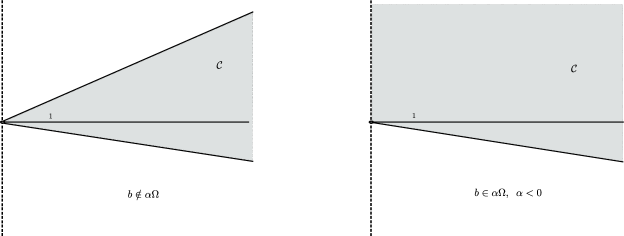
Figure 6: The possibilities for the control set of (4).

We are now able to prove the main result of this section.

3.7 Theorem:

If $b<0$ the unique control set of (4) is $\mathcal{C}$.

Proof.

We will show that $\mathcal{C}=\operatorname{cl}(\mathcal{O}^{+}(x,y))$ for any $(x,y)\in\mathcal{C}$.

Take $(x_{1},y_{1}),(x_{2},y_{2})\in\mathrm{int}\mathcal{C}$ and consider $u_{1},u_{2}\in\mathrm{int}B$, $u_{1}\neq u_{2}$, such that $m_{u_{i}}=y_{i}/x_{i}$, $i=1,2$. Consider also $u\in\Omega$ and $t_{0}>0$ such that $\varphi(t_{0},r_{u_{1}},u)=r_{2}$ and denote $(x_{2}^{\prime},y_{2}^{\prime}):=\varphi(t_{0},(x_{1},y_{1}),u)$.

Assume $m_{u_{1}}m_{u_{2}}<0$. Since this condition is equivalent to $u_{1}u_{2}<0$ we have:

• $u_{1}\alpha<0<u_{2}\alpha$

  • $|(x_{2}^{\prime},y_{2}^{\prime})|\leq|(x_{2},y_{2})|$: Since $\varphi(t,(x_{2},y_{2}),u_{2})=\mathrm{e}^{u_{2}\alpha t}(x_{2},y_{2})$ there exists $t_{1}\geq 0$ such that

    $$\varphi(t_{1},(x_{2},y_{2}),u_{2})=(x_{2}^{\prime},y_{2}^{\prime})\;\;\implies\;\;\varphi(t_{1},\varphi(t_{0},(x_{1},y_{1}),u),u_{2})=(x_{2},y_{2}).$$

    Hence $(x_{2},y_{2})\in\mathcal{O}^{+}(x_{1},y_{1})$;

  • $|(x_{2}^{\prime},y_{2}^{\prime})|>|(x_{2},y_{2})|$: Since $\varphi(t,(x_{1},y_{1}),u_{1})=\mathrm{e}^{u_{1}\alpha t}(x_{1},y_{1})$ and $\lambda:=|(x_{2},y_{2})|/|(x_{2}^{\prime},y_{2}^{\prime})|<1$, there exists $t_{1}>0$ such that $\varphi(t_{1},(x_{1},y_{1}),u_{1})=\lambda(x_{1},y_{1})$. Therefore,

    $$\varphi(t_{0},\varphi(t_{1},(x_{1},y_{1}),u_{1}),u)=\lambda\varphi(t_{0},(x_{1},y_{1}),u)=\lambda(x_{2}^{\prime},y_{2}^{\prime})\in r_{u_{2}}.$$

    However,

    $$|\varphi(t_{0},\varphi(t_{1},(x_{1},y_{1}),u_{1}),u)|=\lambda|(x_{2}^{\prime},y_{2}^{\prime})|=|(x_{2},y_{2})|\implies\varphi(t_{0},\varphi(t_{1},(x_{1},y_{1}),u_{1}),u)=(x_{2},y_{2})$$

    and hence $(x_{2},y_{2})\in\mathcal{O}^{+}(x_{1},y_{1})$.

  
  

• $u_{2}\alpha<0<u_{1}\alpha$

  • $|(x_{2}^{\prime},y_{2}^{\prime})|\geq|(x_{2},y_{2})|$: Since $\varphi(t,(x_{2},y_{2}),u_{2})=\mathrm{e}^{u_{2}\alpha t}(x_{2},y_{2})$ there exists $t_{1}\geq 0$ such that

    $$\varphi(t_{1},(x_{2},y_{2}),u_{2})=(x_{2}^{\prime},y_{2}^{\prime})\;\;\implies\;\;\varphi(t_{1},\varphi(t_{0},(x_{1},y_{1}),u),u_{2})=(x_{2},y_{2})$$

    and hence $(x_{2},y_{2})\in\mathcal{O}^{+}(x_{1},y_{1})$;

  • $|(x_{2}^{\prime},y_{2}^{\prime})|<|(x_{2},y_{2})|$: Since $\varphi(t,(x_{1},y_{1}),u_{1})=\mathrm{e}^{u_{1}\alpha t}(x_{1},y_{1})$ and $\lambda:=|(x_{2},y_{2})|/|(x_{2}^{\prime},y_{2}^{\prime})|>1$, there exists $t_{1}>0$ such that $\varphi(t_{1},(x_{1},y_{1}),u_{1})=\lambda(x_{1},y_{1})$. Therefore,

    $$\varphi(t_{0},\varphi(t_{1},(x_{1},y_{1}),u_{1}),u)=\lambda\varphi(t_{0},(x_{1},y_{1}),u)=\lambda(x_{2}^{\prime},y_{2}^{\prime})\in r_{u_{2}}.$$

    However,

    $$|\varphi(t_{0},\varphi(t_{1},(x_{1},y_{1}),u_{1}),u)|=\lambda|(x_{2}^{\prime},y_{2}^{\prime})|=|(x_{2},y_{2})|\implies\varphi(t_{0},\varphi(t_{1},(x_{1},y_{1}),u_{1}),u)=(x_{2},y_{2})$$

    and hence $(x_{2},y_{2})\in\mathcal{O}^{+}(x_{1},y_{1})$.

Let us assume now that $m_{u_{1}}m_{u_{2}}>0$. Again, this condition is equivalent to $u_{1}u_{2}>0$. Let us analyze the case where $u_{1}\alpha<0\;\;\mbox{ and }\;\;u_{2}\alpha<0$, since the other possibility is analogous.

In this case, by considering $u\in\mathrm{int}B$ with $u\alpha>0$ we have by the proof of the Lemma 3.5 that

$$\frac{\varphi_{2}(t,(x_{1},y_{1}),u)}{\varphi_{1}(t,(x,y),u)}\rightarrow m_{u},\;\;t\rightarrow+\infty\;\;\implies\;\;\frac{\varphi_{2}(t,(x,y),b\alpha^{-1})}{\varphi_{1}(t,(x,y),u)}>0,\;\;\mbox{ for some }t>0.$$

By the above, we have that

$$(x_{2},y_{2})\in\mathcal{O}^{+}(\varphi(t,(x_{1},y_{1}),u))\;\;\;\mbox{ and hence }\;\;\;(x_{2},y_{2})\in\mathcal{O}^{+}(x_{1},y_{1})$$

By the arbitrariness of the choosen points, we obtain $\mathrm{int}\mathcal{C}\subset\mathcal{O}^{+}(x,y)$ for any $(x,y)\in\mathrm{int}\mathcal{C}$. Since $\mathcal{C}$ is closed, we get $\mathcal{C}\subset\operatorname{cl}(\mathcal{O}^{+}(x,y))$ for all $(x,y)\in\mathrm{int}\mathcal{C}$. On the other hand, if $(x,y)\in\mathcal{C}$ and $u\in\mathrm{int}B$, by the proof of Lemma 3.5 $\varphi(t,(x,y),u)\in\mathrm{int}\mathcal{C}$ and consequently

$$\mathcal{C}\subset\operatorname{cl}(\mathcal{O}^{+}(\varphi(t,(x,y),u)))\subset\operatorname{cl}(\mathcal{O}^{+}(x,y))\subset\mathcal{C}\;\;\implies\;\;\mathcal{C}=\operatorname{cl}(\mathcal{O}^{+}(x,y)),\;\;(x,y)\in\mathcal{C}$$

showing that $\mathcal{C}$ is a control set.

Now we prove the uniqueness of $\mathcal{C}$. If

$$\mathcal{C}_{1}:=\{(x,y)\in G;\;y<m_{u_{*}}x\}\;\;\;\mbox{ and }\;\;\;\mathcal{C}_{2}:=\{(x,y)\in G;\;y>m_{u_{*}}x\}$$

we have that

$$G\setminus\mathcal{C}=\left\{\begin{array}[c]{cc}\mathcal{C}_{1}\cup\mathcal{C}_{2}&\mbox{ if }b\notin\alpha\Omega,\\ \mathcal{C}_{1}&\mbox{ if }\;\;b\in\alpha\Omega\;\;\mbox{ and }\;\;\alpha<0\\ \mathcal{C}_{2}&\mbox{ if }\;\;b\in\alpha\Omega\;\;\mbox{ and }\;\;\alpha>0\end{array}\right.$$

Let $(x,y)\in\mathcal{C}_{1}$ and assume that $\varphi(t,(x,y),u)\in\mathcal{C}_{1}$ for some $u\in\mathcal{U}$ and $t>0$. Then, if $(x_{t},y_{t})=(\varphi_{1}(t,(x,y),u),\varphi_{2}(t,(x,y),u)$, Proposition 3.3 gives that

$$\varphi(s,\varphi(t,(x,y),u),u^{\prime})=\varphi(s,(x_{t},m_{u_{*}}x_{t}),u^{\prime})+(0,\mathrm{e}^{bs}(y_{t}-m_{u_{*}}x_{t}))$$

implying that

$$|\varphi(s,\varphi(t,(x,y),u),u^{\prime})-\varphi(s,(x_{t},m_{u_{*}}x_{t}),u^{\prime})|=\mathrm{e}^{bs}\left|\varphi_{2}(t,(x,y),u)-m_{u_{*}}\varphi_{1}(t,(x,y),u)\right|$$

$$=\mathrm{e}^{bs}\bigl{(}m_{u_{*}}\varphi_{1}(t,(x,y),u)-\varphi_{2}(t,(x,y),u)\bigr{)}\leq\mathrm{e}^{b(s+t)}m_{u_{*}}x-y.$$

However, $(x_{t},m_{u_{*}}x_{t})\in\mathcal{C}$ and $\mathcal{C}$ is positively-invariant, hence

$$\varphi(s,\varphi(t,(x,y),u),u^{\prime})\in N_{\epsilon(t)}(\mathcal{C}),\;\;\mbox{ where }\;\;\epsilon(t)=\mathrm{e}^{bt}m_{u_{*}}x-y>0.$$

Since $s>0$ and $u^{\prime}\in\mathcal{U}$ where arbitrary, we have that (see Figure 7)

$$\mathcal{O}^{+}(\varphi(t,(x,y),u))\subset N_{\varepsilon(t)}(\mathcal{C}).$$ (7)

Consequently, if $\widetilde{\mathcal{C}}$ is a control set and there exists $(x,y)\in\widetilde{\mathcal{C}}\cap\mathcal{C}_{1}\neq\emptyset$, by the controlled invariance of $\widetilde{\mathcal{C}}$ there exists $u\in\mathcal{U}$ such that $\varphi(t,(x,y),u)\in\widetilde{\mathcal{C}}$ for any $t>0$. If there is $t_{0}>0$ such that $\varphi(t_{0},(x,y),u)\in\mathcal{C}$ then $\widetilde{\mathcal{C}}\subset\operatorname{cl}\mathcal{O}^{+}(\varphi(t_{0},(x,y),u))=\mathcal{C}$. On the other hand, if $\varphi(t,(x,y),u)\notin\mathcal{C}$ for any $t>0$ then $\varphi(t,(x,y),u)\in\mathcal{C}_{1}$ for any $t>0$. By equation 7 we get

$$\widetilde{\mathcal{C}}\subset\bigcap_{t>0}\mathcal{O}^{+}(\varphi(t,(x,y),u))\subset\bigcap_{t>0}\operatorname{cl}(N_{\epsilon(t)}(\mathcal{C}))=\mathcal{C},$$

where we used that $\mathcal{C}$ is closed and that $\epsilon(t)\rightarrow 0$ as $t\rightarrow+\infty$. In any case we must have $\widetilde{\mathcal{C}}\subset\mathcal{C}$ implying $\mathcal{C}_{1}\cap\mathcal{C}\neq\emptyset$ which is a contradiction since $\mathcal{C}_{1}\subset G\setminus\mathcal{C}$. Therefore, there is no control set intersecting $\mathcal{C}_{1}$.

In an analogous way we show that there is no control set intersecting $\mathcal{C}_{2}$ and therefore $\mathcal{C}$ is the only control set, concluding the proof. ∎

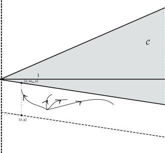
Figure 7: An $\epsilon(t)$-neighborhood of $\mathcal{C}$ and the behavior of the solutions outside $\mathcal{C}$.

3.8 Remark:

Let us notice that the previous result shows that $\Sigma$ admit exactly one control set and it has nonempty interior. For more general Lie groups, the authors showed in [2] that linear control systems admits, under strong topological conditions, exactly one control set with nonempty interior. However, there are no information about the control sets with empty interior.

3.5 Automorphisms of $G$ and control sets

By the calculations in the previous sections, any arbitrary linear control system on $G$ is conjugated to one of the linear control systems (1), (2), (ref3) or (4) by an automorphism. Therefore, the control sets of $\Sigma$ can be reobtained from the control sets of the above system by considering the preimage of the automorphism in question.

With that in mind we have the following geometric view of the control sets of $\Sigma$.

3.9 Theorem:

For the linear control system $\Sigma$ it holds:

• $\alpha=a\alpha+b\beta=0$ and any vertical line close to $(1,0)$ is a control set;

• $\alpha=0$ and $a\alpha+b\beta\neq 0$, and the control sets are vertical segments intersecting

  $$\{(x,y)\in G;\;y=-ab^{-1}(x-1)\};$$

• $\alpha\neq 0$ and $a\alpha+b\beta=0$, and $\Sigma$ admits only the control set

  $$\{(x,y)\in G;\;y=\beta\alpha^{-1}(x-1)\};$$

• $\alpha(a\alpha+b\beta)\neq 0$ with $b=0$ and the unique control set is the whole $G$;

• $\alpha(a\alpha+b\beta)\neq 0$ with $b\neq 0$ and the unique control set is a cone in $G$ with (open) edge on the point $(0,ab^{-1})$.

The proof of the previous result is straightforward and follows directly from the following facts concerning an arbitrary automorphism. Let $\psi(x,y)=(x,c(x-1)+dy)$ be an automorphim of $G$. It holds:

• If $r\subset G$ is a ray, $\psi(r)=l\cap G$ where $l$ is a line passing by $(0,-c)$;

• $\psi$ preserves any vertical line in $G$.

References

• [1] V. Ayala and A. Da Silva, Controllability of Linear Control Systems on Lie Groups with Semisimple Finite Center, SIAM Journal on Control and Optimization 55 No 2 (2017), 1332-1343.
• [2] V. Ayala, A. Da Silva and G. Zsigmond, Control sets of linear systems on Lie groups. Nonlinear Differential Equations and Applications - NoDEA 24 No 8 (2017), 1 - 15.
• [3] V. Ayala and L.A.B. San Martin, Controllability properties of a class of control systems on Lie groups, Lecture Notes in Control and Information Sciences 258 (2001), 83 - 92.
• [4] V. Ayala and J. Tirao, Linear control systems on Lie groups and Controllability, Eds. G. Ferreyra et al., Amer. Math. Soc., Providence, RI, 1999.
• [5] V. Ayala and L. San Martin. Controllability of $2$-dimensional Bilinear Systems: Restricted Controls, Discrete-Time. Proy, Vol. 18, pp. 207-223, 1999.
• [6] F. Colonius and W. Kliemann, The Dynamics of Control, Birkhäuser, Boston, 2000.
• [7] A. Da Silva, Controllability of linear systems on solvable Lie groups, SIAM Journal on Control and Optimization 54 No 1 (2016), 372-390.
• [8] M. Dath and P. Jouan, Controllability of Linear Systems on Low Dimensional Nilpotent and Solvable Lie Groups, Journal of Dynamics and Control Systems 22 N0 2 (2016), 207-225.
• [9] Ph. Jouan, Controllability of linear systems on Lie group, J. Dyn. Control Syst. 17 (2011), 591-616.
• [10] Ph. Jouan, Equivalence of Control Systems with Linear Systems on Lie Groups and Homogeneous Spaces, ESAIM: Control Optimization and Calculus of Variations, 16 (2010) 956-973.
• [11] U. Ledzewick, H. Shattler, Optimal controls for a two compartment model for cancer chemotherapy with quadratic objective., Proceedings of MTNS (2006), Kyoto,Japan.
• [12] G. Leitmann, Optimization Techniques with Application to Aerospace Systems, Academic Press Inc., London, 1962.
• [13] L. Markus, Controllability of multi-trajectories on Lie groups, Proceedings of Dynamical Systems and Turbulence, Warwick 1980, Lecture Notes in Mathematics 898, 250-265.
• [14] L. S. Pontryagin, V. G. Boltyanskii, R. V. Gamkrelidze and E.F. Mishchenko, The mathematical theory of optimal processes, Interscience Publishers John Wiley & Sons, Inc., New Yor , A. Control and Systems Engineering A Report on Four Decades of Contributions, Studies in Systems, Decision and Control, 2015.
• [15] K. Shell, Applications of Pontryagin’s Maximum Principle to Economics, Mathematical Systems Theory and Economics I and II, Volume 11/12 of the series Lecture Notes in Operations Research and Mathematical Economics (1968), 241-292.