Unsupervised Learnable Sinogram Inpainting Network (SIN) for Limited Angle CT reconstruction

Abstract

In this paper, we propose a sinogram inpainting network (SIN) to solve limited-angle CT reconstruction problem, which is a very challenging ill-posed issue and of great interest for several clinical applications. A common approach to the problem is an iterative reconstruction algorithm with regularization term, which can suppress artifacts and improve image quality, but requires high computational cost.

The starting point of this paper is the proof of inpainting function for limited-angle sinogram is continuous, which can be approached by neural networks in a data-driven method, granted by the universal approximation theorem. Based on this, we propose SIN as the fitting function – a convolutional neural network trained to generate missing sinogram data conditioned on scanned data. Besides CNN module, we design two differentiable and rapid modules, Radon and Inverse Radon Transformer network, to encapsulate the physical model in the training procedure. They enable new joint loss functions to optimize both sinogram and reconstructed image in sync, which improved the image quality significantly. To tackle the labeled data bottleneck in clinical research, we form a sinogram-image-sinogram closed loop, and the difference between sinograms can be used as training loss. In this way, the proposed network can be self-trained, with only limited-angle data for unsupervised domain adaptation.

We demonstrate the performance of our proposed network on parallel beam X-ray CT in lung CT datasets from Data Science Bowl 2017 and the ability of unsupervised transfer learning in Zubal’s phantom. The proposed method performs better than state-of-art method SART-TV in PSNR and SSIM metrics, with noticeable visual improvements in reconstructions.

I Introduction

Limited angle CT reconstruction is a very challenging ill-posed issue and of great interest in several clinical applications, such as digital breast tomosynthesis [1], dental tomography [2], short exposure time [3], etc. In a limited-angle CT scan, the projection data can be obtained in less than $180^{\circ}$ angular range, and the data insufficiency degrades reconstruction quality with streaking artifacts(fig 1 (a)(b)).

(a)

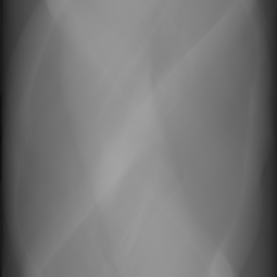
(b)

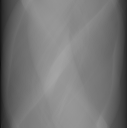
(c)

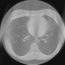
(d)

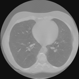
(e)

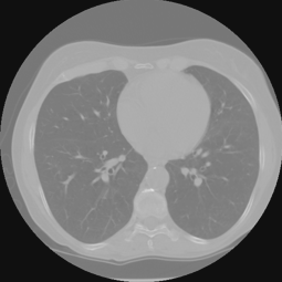
(f)

Figure 1: Qualitative illustration of the task: (a) given a limited-angle sinogram; (b) automatic inpainting result using our sinogram inpainting network (SIN); (c) ground truth sinogram; (d) reconstruction result of state-of-art iterative SART method with TV normalization; (e) our method output; (f) ground truth image

While the uniqueness of solutions for non-truncated limited-angle CT has been proved by analytic continuation theory [4], the academia has not yet found a closed-form solution for the problem. A common approach to the problem is an iterative reconstruction algorithm with regularization term based on compressed sensing theory [5]. The academia has reported some iterative algorithms, e.g. classic ART [6], POCS [7], and some regularization terms, e.g. TV [8], ATV [9]. These algorithms can suppress artifacts and improve image quality but require high computational cost for iterative projections and back-projections.

Another attempt to tackle insufficient data reconstruction problem is sinogram inpainting, which has been explored for recovering incomplete information in projection, e.g. metal artifact reduction (MAR) [10, 11, 12, 13] , sparse-view reconstruction based on dictionary learning [14] , and suppresses ring artifacts caused by detector gaps [15]. However, limited-angle sinogram inpainting remains challenging for large missing regions, which is known as the ”semantic hole-filling” issue. An exemplary algorithm GP-EL [16], which tries to recover the sinogram signal based on a GP extrapolation algorithm, still failed to produce satisfying results. Therefore, the iterative reconstruction remains the state-of-art method.

In recent years, deep learning(DL) [17] has attracted a lot of attention because of convolutional neural networks’(CNN) outstanding performance in image classification [18, 19], object detection [20, 21, 22], and super-resolution [23, 24]. Meanwhile, Deepak Pathak proposed Context Encoders [25], the first network able to give reasonable results for ”semantic hole-filling” issue, which is a promising approach to solve the limited-angle sinogram inpainting task.

Data-driven learning method has been explored in CT field, e.g. a redundant learned dictionary as a CS sparsity normalization term in sinogram inpainting for MAR [14] and low-dose CT reconstruction [26]. CNNs have been showing their huge potential ability in CT reconstruction. Zhang H.M [27] adopted a 3-layer deep neural network on post-processing limited-angle CT FBP reconstruction, with the benefits of artifacts reduction and image details recovery. Kyong H.J. et. [28] proved that iterative methods can be viewed as a CNN and proposed FBPConvNet, FBP reconstruction combined with a U-Net [29] CNN, for sparse-view CT reconstruction. Ge W.’s pilot experiment [30] shows the potential of 3-layer deep network to improve the image and sinogram quality, e.g. inpaint in the sinogram for eliminating metal artifacts. Hu C. et. [31] proposed a ”Residual Encoder-Decoder Convolutional Neural Network” (RED-CNN) to eliminate image noise in low-dose CT.

Despite these works, two practical and theoretical questions remain regarding applying deep learning method in limited-angle CT reconstruction. First one, the network mentioned above focused on either image domain [28, 27, 31] or sinogram domain [30], without cross-domain information transferring during training. So an image domain network may generate results not satisfying data fidelity, and a sinogram domain network inpainting result may have small inconsistency can cause significant artifact in reconstruction. To tackle this problem, cross-domain error backward-propagation is in need, which requires new-designed differentiable reconstruction and projection method embedded in the network. The second one is that networks mentioned above were trained supervised, i.e. with labeled/paired training data. However, labeled data are limited in amount or expensive [30] in the clinical world due to some reasons, like dose or privacy.

In this paper, we start our discussion proving sinogram inpainting function is continuous based on analytic continuation theory, so it can be fitted by the neural networks in data-driven method guaranteed by universal approximation theorem [32]. We propose Sinogram Inpainting Network(SIN), a convolutional neural network trained to generate missing sinogram data conditioned on projections from the scan, as the fitting function. To implement the cross-domain error backward-propagation we propose Radon and Inverse Radon Transformer network. This differentiable module can be inserted into existing convolutional network architectures, which enables to perform CT projection and/or reconstruction within the network. And we adopt an image processing network in our networks to eliminate the artifacts caused by small inconsistency in the inpainted sinogram. The three parts form an end-to-end network from sinogram domain to image domain, with benefits of taking both of image error and sinogram error into account in the sync process in supervised training, i.e with limited-angle/full-view sinogram pairs.

To tackle this training data bottleneck, we develop an unsupervised train method with only limited-angle projection on our proposed network. Inspired by the observation: reconstruction and projection can form a closed loop, we can get a fake projection from the reconstructed image, and the disparity between the fake projection and real projection gives feedback signals to train proposed network unsupervised.

We demonstrate the performance of our proposed network on lung CT datasets from Data Science Bowl 2017, and the ability to unsupervised transfer learning on Zubal’s phantom [33]. The proposed method highly improves limited-angle CT reconstruction quality and performs better than state-of-art method iterative SART with ATV normalization in PSNR and SSIM quantitative metrics. Visual improvements in our results are easily noticeable.

II Method

In this chapter, we will cover why sinogram inpainting task can be implemented by neural network, what architecture of neural network is adapted to the task and how to train the neural network. We start by proving sinogram inpainting task is a continuous function of original projection. Going on, we demonstrate the three parts and their contributions in the proposed network:sinogram inpainting network, radon/inverse radon transfer module and image processing network. Finally, we defines the training objective and loss function for supervised and unsupervised training.

II-A Theory

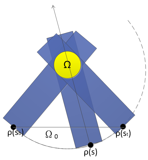
(a)

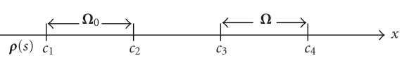
(b)

Figure 2: a) Illustration of parallel-beam limited angle scanning geometry, where solid line is the trajectory of source $\rho$ and dashed line represents the missing data; (b) 1D coordinate along the x-ray source path indicated in (a).

For the continuous nontruncated limited-angle problem, we use parallel-beam case as a representative, illustrated in Figure 2, and the following proof applies equally to fan-beam case. Object function $f(\mathbf{x})$ is constrained in a compact support $\Omega\subset\mathbb{R}^{2}$, and $\Gamma$ is a general smooth source trajectory.

$$\Gamma=\{\rho(s)|s\in\mathbb{R}\}$$ (1)

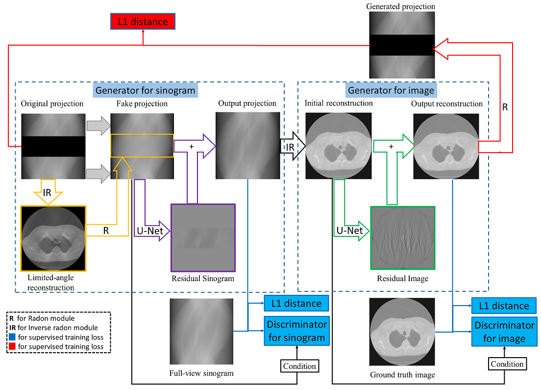
Figure 3: Architecture of the proposed network. The $G_{s}$ is residual. The blue blocks denote the loss for supervised training and the red blocks denote the loss for unsupervised training.

Two points $\rho(s_{b})$ and $\rho(s_{t})$ are start and terminal points of the We begin our discussion by proving describing our on continuous case. limited scanning, $\rho(s)$ is any point satisfying $s_{b}<s<s_{t}$ , and the dashed line represents missing data with point $\rho(\tilde{s})$ on it. Assuming that connecting $\rho(s_{b})$ and $\rho(s_{t})$ forms a measurable region $\Omega_{0}$, we can set 1D coordinate along any X-ray $(s,\theta)$ intersects $\Omega$ from $\rho_{s}$, and we denote points where the X-ray intersects with $\Omega_{0}$ and $\Omega$ as $c_{1},c_{2},c_{3},c_{4}$ , with $c_{1}<c_{2}<c_{3}<c_{4}$

Based on the inverse Hilbert Transform [34], we have the reconstructiont formulation for $f(x)$ from the research of Yangbo Y. [4] , where $g(x)$ is the 1D Hilbert transform of $f(x)$

$$\begin{split}&\sqrt{(c_{4}-x)(x-c_{1})}f(x)\\ &=\int_{c_{1}}^{c_{2}}\frac{\sqrt{(c_{4}-\tilde{x})(\tilde{x}-c_{1})}g(\tilde{x})}{\pi(\tilde{x}-x)}d\tilde{x}+\frac{1}{\pi}\int_{c_{3}}^{c_{4}}f(\tilde{x})d\tilde{x}\\ &+\int_{c_{2}}^{c_{4}}\frac{\sqrt{(c_{4}-\tilde{x})(\tilde{x}-c_{1})}g(\tilde{x})}{\pi(\tilde{x}-x)}d\tilde{x}\end{split}$$ (2)

Pack et al. [35] presents a local operation for converting projections into values of $g(\tilde{x})$. We use $\mathcal{L}$ to represent the coverting operator for clarity, and $P$ to be the scanning projection data.

$$g(\tilde{x})=\mathcal{L}(P,\tilde{x})~{},~{}~{}x\in(c_{1},c_{2})$$ (3)

We denote the last part of equation 2 as $G_{c_{2}c_{4}}$. For $f(x)|_{x\in(c_{1},c_{2})}=0$

$$\begin{split}&G_{c_{2}c_{4}}(x)|_{P,x\in(c_{1},c_{2})}\\ &=\int_{c_{2}}^{c_{4}}\frac{\sqrt{(c_{4}-\tilde{x})(\tilde{x}-c_{1})}g(\tilde{x})}{\pi(\tilde{x}-x)}d\tilde{x}\\ &=-\int_{c_{1}}^{c_{2}}\frac{\sqrt{(c_{4}-\tilde{x})(\tilde{x}-c_{1})}g(\tilde{x})}{\pi(\tilde{x}-x)}d\tilde{x}-\frac{1}{\pi}\int_{c_{3}}^{c_{4}}f(\tilde{x})d\tilde{x}\\ &=-\int_{c_{1}}^{c_{2}}\frac{\sqrt{(c_{4}-\tilde{x})(\tilde{x}-c_{1})}\mathcal{L}(P,\tilde{x})}{\pi(\tilde{x}-x)}d\tilde{x}-\frac{1}{\pi}P(s,\theta)\end{split}$$ (4)

As [4] pointed out, $G_{c_{2}c_{4}}(x)|_{P}$ is an analytic function with a cut on $[c_{2},c_{4}]$, so it can be extended to $[c_{2},c_{4}]$ as a continuous function, denoted as $\mathcal{E}G_{c_{2}c_{4}}|_{P}$. Then we can get f(x) following equation 2

$$\begin{split}f(x)|_{P,x\in(c_{3},c_{4})}=\frac{\frac{P(s,\theta)}{\pi}+\mathcal{E}G_{c_{2}c_{4}}(x)|_{P}+L(x)|_{P}}{\sqrt{(c_{4}-x)(x-c_{1})}}\\ L(x)|_{P}=\int_{c_{1}}^{c_{2}}\frac{\sqrt{(c_{4}-\tilde{x})(\tilde{x}-c_{1})}\mathcal{L}(P,\tilde{x})}{\pi(\tilde{x}-x)}d\tilde{x}\end{split}$$ (5)

We can use Radon Transform, denoted as $\mathcal{R}$, to get the missing projection data $\tilde{P}$.

$$\begin{split}\tilde{P}&=\mathcal{R}f(x)|_{P}\\ &=\int_{\tilde{s},\tilde{\theta}}\frac{\frac{P(s,\theta)}{\pi}+\mathcal{E}G_{c_{2}c_{4}}(x)|_{P}+L(x)|_{P}}{\sqrt{(c_{4}-x)(x-c_{1})}}\mathrm{d}x\\ &=F(P)\end{split}$$ (6)

So we have proven the sinogram inpainting target $\tilde{P}$ is a function of scanning data $F(P)$.Because $\mathcal{L}(P,\tilde{x})$, $G_{c_{2}c_{4}}(P,x)$ and $\mathcal{E}$ are all continuous on $P$, so the $F(P)$ is continuous on $P$.

Based on universal approximation theorem [32] , a feed-forward network with a single hidden layer containing a finite number of neurons can be used to approximate continuous functions on compact subsets of $\mathbb{R}^{n}$. As $\mathbb{C}$ can be viewed as $\mathbb{R}^{2}$, the conclusion also applies to our function. So we propose a deep network trained to generate missing sinogram data conditioned on projections from scan.

II-B Network Design

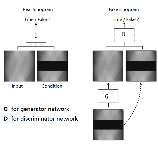
Figure 4: Sinogram inpainting network is a conditional GAN. The discriminator D learns to identify real and fake sinogram. The generator learns inpaint the sinogram to fool the discriminator. The limited angle projection is used twice as condition.

Based on the proof in II-A, it’s possible to train an end-to-end neural network from sinogram to reconstruction image, but requires the network to encode the conversion from polar coordinate to the rectangular coordinates by learning [28]. So we seperate the process into three parts: the sinogram inpainting network (SIN, shown in fig 5), radon/inverse radon transformer module (shown in fig 6), and image processing network. This configuration keeps SIN network only processing sinogram information and so does image processing network in image domain, which simplifies the network architecture and reduce learning complexity.

The network architecture is shown in fig 3 and the effect of each part is demonstrated in fig 8. First we introduce the network parts and its effect in supervised training. In the last part, we will introduce the unsupervised training method.

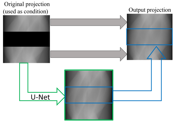
(a)

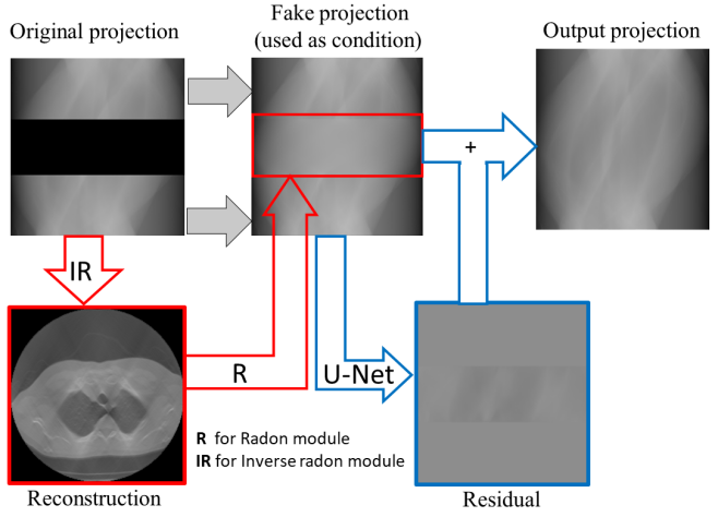
(b)

Figure 5: two different architecture of the generator network for sinogram inpainting, (a) is called non-residual $G_{s}$ and (b) is the proposed one and called residual $G_{s}$.

II-B1 Sinogram Inpainting Network

In this paper, we base our sinogram inpainting network on pix2pix network [36], concluding two parts: the generator $G_{s}$ and the conditional discriminator $D_{s}$, where $G_{s}$ takes limited-angle sinogram as input and generates fake images that fool $D_{s}$, and $D_{s}$ tries to discriminate real and fake images based on the condition image. $D_{s}$ is only used in supervised training.

We use pix2pix network to replace Context Encodes base network for two reasons: i) pix2pix adds skip connection in the generator like ”U-Net” [29], so the low-level feature can be shuttled directly, which is a good analog for multiresolution single reconstruction. ii) pix2pix uses conditional adversarial networks instead of traditional adversarial network( shown in 4), so it can learn a conditional generative model with a conditional loss function based on the input condition when we condition on the input sinogram in our case.

As a refinement of pix2pix, we use the original data to replace corresponding part in fake images, which forces the $G_{s}$ focusing on learning the missing part. And we compairs two different types of generator(as shown in 5), one tries to generate the missing data from the original data directly, which is called non-residual $G_{s}$. The other one reconstructs image with limited-angle arifacts and generates the fake projection data for missing angle firstly, and try to learn the difference between the fake projection and ground truth. We can see the residual $G_{s}$ performs better in experiment (shown in fig 7) , for reconstruction and projection process encapsulates the physical model and preserves some information.

II-B2 Radon and inverse radon module

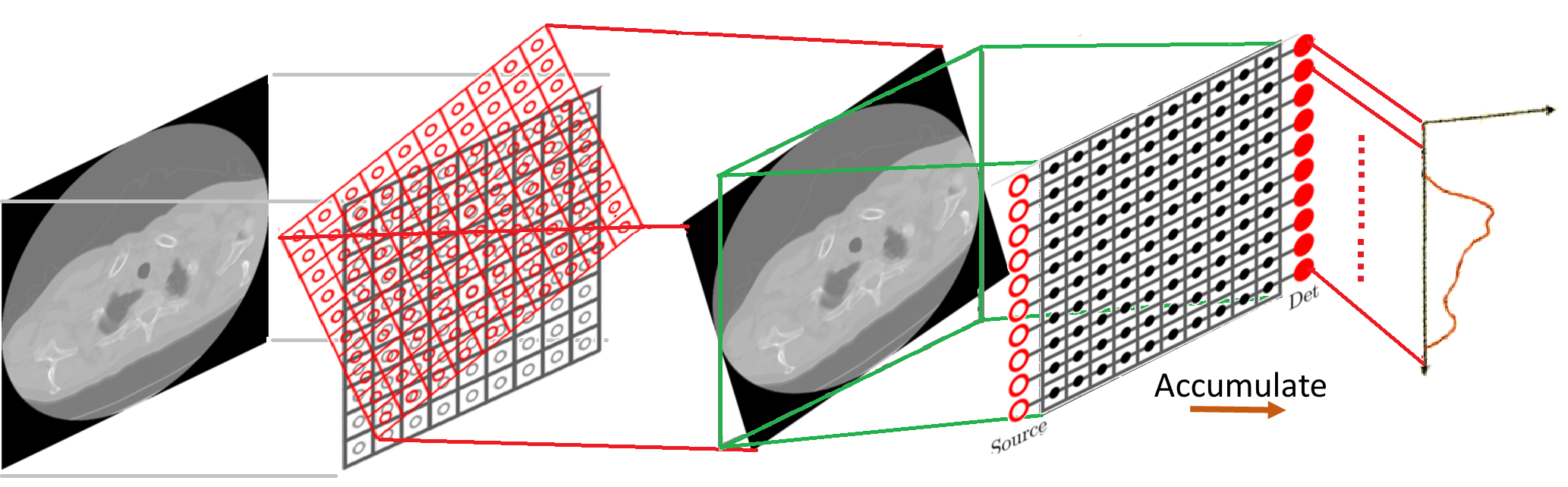
(a)

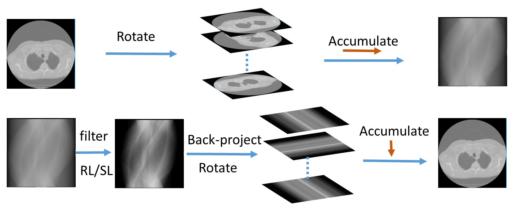
(b)

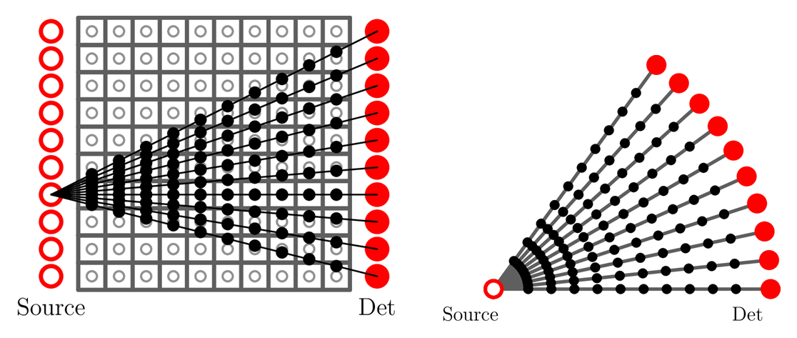
(c)

Figure 6: Illustration of Radon Transformer and Inverse Radon Transformer network(a) The interpolation and accumulation process; (b) The Radon transformer can be viewed as rotate interpolation and accumulation. The inverse Radon transformer can be viewed as: 1D filtering(SL, RL ,etc.), interpolation, and accumulation; (c) This module can be easily extended to other geometry, e.g. equal-distance and equal-angle fan-beam.

As we all know, minor inconsistencies in sinogram may lead to serious artifacts in the reconstructed image. It’s benefical to take both of image error and sinogram error in account in training, which requires a reconstruction module with the ability for error backward-propagation from image domain to sinogram domain. So iterative methods are not suitable.

And it’s challenging to deploy FBP reconstruction method in neural network, because traditional implement of FBP requires the mulitplication of huge system matrix. It will take too much space if stored in dense array, (for a $256*256$ reconstruction image detected by $256$ detector pixels in $360$ views, the array size is 24.16GB in float32 type , the sparsity is approximate $0.0078$). On the other hand, compution on sparse array is time-consuming for forward and backward propagation.

We propose a differentiable Radon transformer network $\mathcal{R}$ and inverse Radon transformer network $\mathcal{\tilde{R}}$ with the ablity or error backward-propagation, to replace system matrix mulitplication(shown in fig 6). The Radon transformer,i.e. parallel-beam projection, can be seperated by two parts: interpolation (inspired by spatial transformer network [37]), and accumulation. The inverse Radon transformer, i.e. parallel-beam reconstruction, concluded: 1D filtering(SL, RL ,etc.), interpolation, and accumulation. The system matrix coefficients are replaced by densely stored interpolation coefficients. This module can be easily extended to other geometry, e.g. fan-beam, cone-beam.

This differentiable module can be inserted into existing convolutional architectures, which enables to perform CT projection and/or reconstruction within the network and the optimisation process.

II-B3 Image processing network

As mentioned before, some reconstruction artifacts are corresponding to minor inconsistencies in sinogram. The idea is natural to eliminate these arifacts in image domain more easily than in sinogram domain, so it should be benefical to have an deep network for image processing. We still base image processing network on pix2pix, where the generator is denoted as $G_{i}$, the discriminator is $D_{i}$, and FBP reconstruction image from original limited angle sinogram as condition. $D_{i}$ is only used in supervised training.

As a modification, we add a skip connection between $G_{i}$ input and output, like [28, 23]. So $G_{i}$ only learns the residual part $\mathbf{r}=\mathbf{y}-\mathbf{x}$, which release the network from preserving all information. At the same time, the skip connection makes the $G_{s}$ easier to optimize by providing a short-cut way for error backward-propagation and tackles the vanishing/exploding gradients problem , like in Resnet [18].

The generator part of this network is very similar to [28], but we add discriminator and adversarial loss, which is benefical for restore high-frequency structure [25, 36],

II-B4 Unsupervised transfer learning

In some practical scene, paired training data, i.e. limited-angle projection and full-view projection/ground truth image, is limited in amount or very costly. $D_{s},D_{i}$ can’t work without paired data, which limits the applicable scene for the supervised training method. To tackle training data bottleneck, we develop a unsupervised transfer training method with only limited angle projection.

Inspired by dual-learning [38], CT imaging can be view as a dual task: reconstruction and projection can form a closed loop. With only limited angle projection sinogram, we can reconstuct an image using $G_{s}$, inverse radon transformer and $G_{i}$. So we can project reconstructed image by radon transformer network, and the disparity between the generated projection and original projection data gives feedback signals to train proposed network unsupervisedly. The objective shown as red block in fig 3.

II-C Objective

In supervised training case, our Loss function objective is the weighted sum of cGAN objective and a traditional L1 distance, suggested by [25, 36] . The objective of a conditional GAN can be expressed as [25],

$$\begin{split}\mathcal{L}_{c,G_{s}}(G_{s},D_{s})=&\mathbb{E}_{x,y\sim p_{s}(x,y)}[logD_{s}(x,y)]\\ +\mathbb{E}_{x,y\sim p_{s}(x,y)}[&log(1-D_{s}(x,G_{s}(x))]\\ \mathcal{L}_{c,G_{i}}(G_{i},D_{i})=&\mathbb{E}_{x,y\sim p_{s}(x,y)}[logD_{i}(\mathcal{\tilde{R}}(G_{s}(x)),\mathcal{\tilde{R}}(y))]\\ +\mathbb{E}_{x,y\sim p_{s}(x,y)}&[log(1-D_{i}(\mathcal{\tilde{R}}(G_{s}(x)),G_{i}(\mathcal{\tilde{R}}(G_{s}(x))))]\end{split}$$ (7)

where $p_{s}$ denotes data distribution, x is limited-angle sinogram data and y is full-view data. $D_{s},D_{i}$ tries to discriminates real and fake data by maximizing the loss and $G_{s},G_{i}$ tries to fool the discriminator by minimizing the loss, i.e. $G_{s}^{*},G_{i}^{*}=\arg\min_{G_{i},G_{s}}\max_{D_{i},D_{s}}[\mathcal{L}_{c,G_{s}}(G_{s},D_{s})+\lambda_{i}\mathcal{L}_{c,G_{i}}(G_{i},D_{i})]$

The $L_{1}$ loss plays the role like data fidelity items in image reconstuction, keeping the generated data close the ground truth.

$$\mathcal{L}_{L1,G_{s}}(G_{s}) =\mathbb{E}_{x,y\sim p_{s}(x,y)}[||y-G_{s}(x)||_{1}]$$ (8)

$$\mathcal{L}_{L1,G_{i}}(G_{i}) =\mathbb{E}_{x,y\sim p_{s}(x,y)}[||\mathcal{\tilde{R}}(y)-G_{i}(\mathcal{\tilde{R}}(x))||_{1}]$$ (9)

The final loss fuction and objective are

$$\begin{split}\mathcal{L}=&\lambda_{i}(\mathcal{L}_{c,G_{i}}(G_{i},D_{i})+\lambda_{L}\mathcal{L}_{L1,G_{i}}(G_{i}))\\ &+\mathcal{L}_{c,G_{s}}(G_{s},D_{s})+\lambda_{L}\mathcal{L}_{L1,G_{s}}(G_{s}))\\ G_{s}^{*},G_{i}^{*}=&\arg\min_{G_{i}}\max_{D_{i}}\min_{G_{s}}\max_{D_{s}}\mathcal{L}\end{split}$$ (10)

For unsupervised transfer training case,

$$\begin{split}\mathcal{L}=&\mathbb{E}_{x\sim p_{s}(x)}||(1-M)\odot(x-\mathcal{R}G_{i}\mathcal{\tilde{R}}G_{s}x)||_{1}\\ G_{s}^{*},G_{i}^{*}=&\arg\min_{G_{i}}\min_{G_{s}}\mathcal{L}\end{split}$$ (11)

where $\odot$ is the element-wise product operation, $p_{s}$ denotes data distribution, $x$ is limited-angle sinogram data and $M$ is limited-angle mask. The loss plays the role of data fidelity items and aims to eliminate data inconsistencies.

III Results

In this chapter, we will introduce our datasets, experiment setup and results. In this paper, our experiments focus on parallel CT, but the method is general and can be easily modified to apply in fan-beam CT as metioned before. We compair the proposed method to FBP alone and state-of-the-art iterative reconstrucion method with TV normalization [8], denoted as SART-TV.

III-A Datasets and Experiment Configuration

We demonstrate the performance of our proposed network on two datasets: lung CT datasets(fig 9) from Data Science Bowl 2017 for supervised training and test, and

Zubal’s phantom CT data (fig 9) from neck to mid-thigh, except lung position, for test the ability of unsupervised transfer learning. The lung CT train set is with 6312 images (from 38 persons) and test set is with 113 images(from 2 persons). The Zubal’s unsupervised test set is 40 images of 1 person.

Our data preparation goes as follows: firstly normlize the input image value range to be [-1, 1] and image size to be $256\times 256$, and take this as ground truth image. The we generate the projection using $\mathcal{R}$ for 256 views in $180\deg$ with 256 detectors with the same size of image pixel, taken as ground truth projection. The we cut the middle $60\deg$ projection out(86 views), taken as the limited-angle projection input.

We use the Pytorch toolbox (ver. 0.2.0) to implement the proposed network including SIN. And we use a Tesla P100 graphic card (NVIDIA Corporation) for train and test. The hyperparameters for training are as follows: we use the adam optimizer of all of $G_{i},G_{s},D_{i},D_{s}$, learning rate decreasing linearly from 0.002 to 0, the momentum $\beta_{1}$ equals 0.5, $\beta_{2}$ 0.999; batchsize is 30. The SART hyperparameters are tuned manually to ge the best performance in average, because it’s the common practice in general and the academia haven’t come to the common idea of data-driven parameters setting method. We finally set the 60 iteration for each image, and in each epoch we take 20 steps of TV with the factor $\alpha=0.06,\alpha_{s}=0.997$.

III-B Comparsion With Different Architecture

We take two samples from lung CT test set to demonstrate the difference corresponded to changes in network architecture.

Firstly, the inpainting results of non-residual/residual sinogram generator work is shown in fig 7. And the sinogram of non-residual $G_{s}$ has much more inconsistence than residual one as non-residual needs to keep more information through network.

(a)

(b)

(c)

(d)

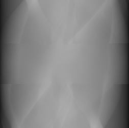
(e)

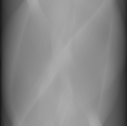
(f)

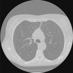
(g)

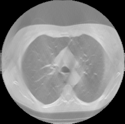
(h)

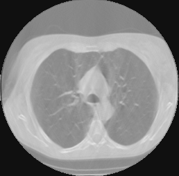
(i)

Figure 7: Demonstrates inpainting results for different $G_{s}$ architecture a) the original limited-angle data; b) FBP reconstruction image for a); c) use projection from b) to replace the missing data in a); d) the ground truth of sinogram;e) the output of non-residual $G_{s}$ with a) as input; f) the output of residual $G_{s}$ with c) as input;g) the ground truth of reconstruction image; h) FBP reconstruction for e); i) FBP reconstruction for f).

Secondly, comparison of reconstruction results eliminating different part in our Network is shown in fig 8, which helps demonstrate the individual contribution of the elements. For example, comparing fig 8 (d) and (f) tells us the $G_{i}$ can eliminate the artifacts due to sinogram inconsistence so small to tackle, as we imagined. Result for eliminating the $G_{s}$ and taking the FBP reconstructed images as $G_{i}$ input, shown in fig 8 (e) , which is similar to the architecture in [28] , suffers image quality degradation due to the blurring and artifacts introduced by the filtering process in FBP.

(a)

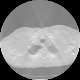
(b)

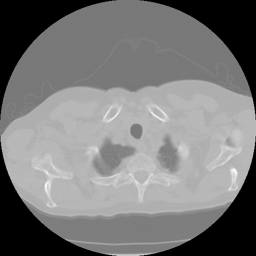
(c)

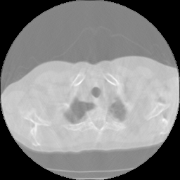
(d)

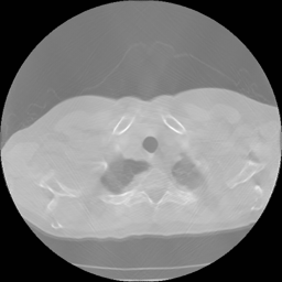
(e)

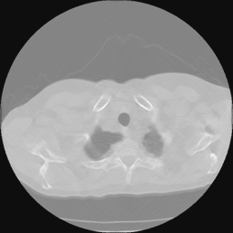
(f)

Figure 8: Demonstrates reconstruction results eliminating different part in our Network. a) the original limited-angle data; b) FBP reconstruction image for a); c) the ground truth of reconstruction image; d) Eliminate the $G_{i}$ part, i.e. reconstruction from $G_{s}$ output; e) Eliminate $G_{s}$, and train $G_{i}$ with b) as input, like [28] ; f) the output of residual $G_{s}$ with c) as input.

III-C Quantitative Metrics and Experimental Results

We choose two quantitative metric to measure the quality of reconstruction: peak signal to noise ratio (PSNR), and the mean structural similarity index (SSIM) with the ground truth images. If $x$ denotes the ground truth $\hat{x}$ denotes the algorithm output, PSNR and SSIM are given by

$$\hbox{PSNR}(\hat{x},x)=20\cdot\log\frac{\mathcal{R}_{x}}{\sqrt{\mathrm{E}(\hat{x}-x)^{2}}}$$ (12)

$$\hbox{SSIM}(\hat{x},x)={\frac{(2\mathrm{E}_{\hat{x}}\mathrm{E}_{x}+c_{1})(2\sigma_{{\hat{x}x}}+c_{2})}{(\mathrm{E}_{\hat{x}}^{2}+\mathrm{E}_{x}^{2}+c_{1})(\sigma_{\hat{x}}^{2}+\sigma_{x}^{2}+c_{2})}}$$ (13)

where $\mathcal{R}_{x}$ denotes the range of x, i.e. $x_{\max}-x_{\min}$, $\mathrm{E}$ denotes the average, $\sigma^{2}$ denotes the variance. $\sigma_{xy}$ denotes the covariance of $x$ and $y$, $c_{1}=(0.01\mathcal{R}_{x})^{2}$, $c_{2}=(0.03\mathcal{R}_{x})^{2}$ .It’s easy to see PSNR estimates absolute errors and SSIM is more sensitive for changes in structural information. Both higher PSNR and SSIM values correspond to better reconstruction.

III-C1 Lung CT Test datasets

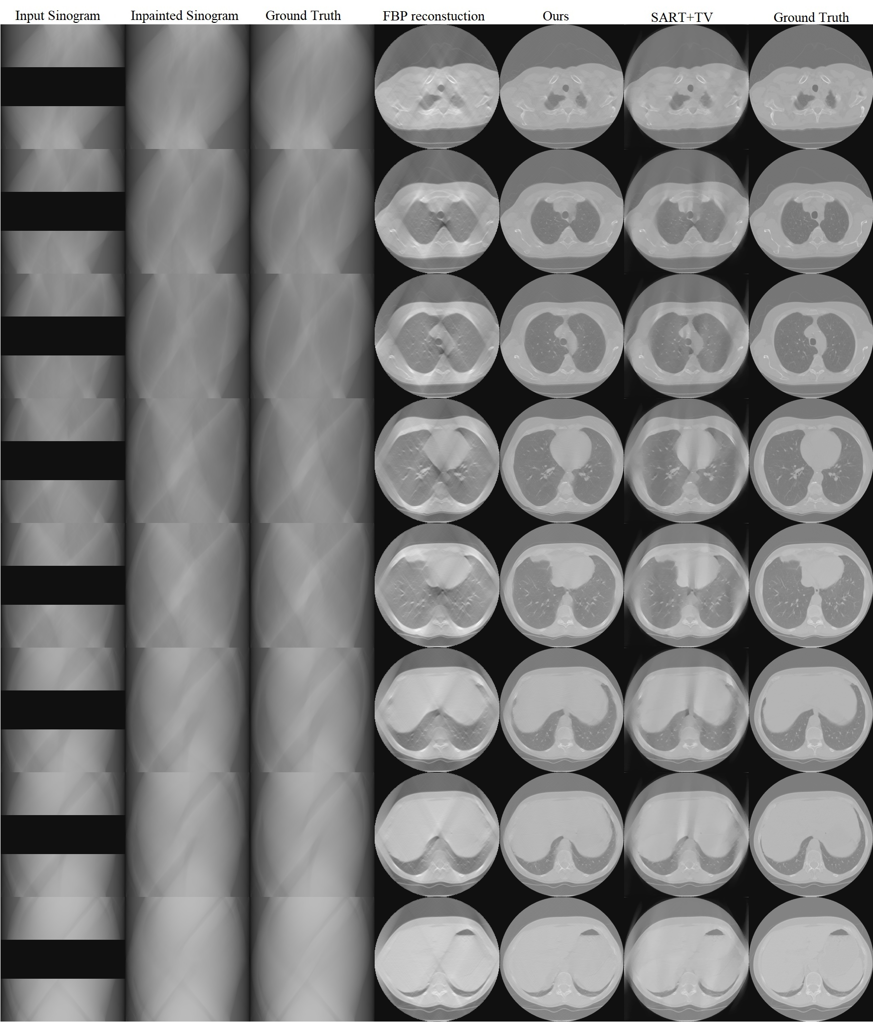
Figure 9: The inpainted sinogram and reconstructed images for test datasets of lung CT from Data Science Bowl 2017. We compair three reconstrucion methods: FBP, our proposed supervised-trained network, and iterative SART reconstrucion with TV regularization. Both the proposed network and SART-TV method reduce the streaking artifacts. And our results have less cartoon-like artifacts than SART-TV. The display window is [-1, 1].

Fig 9 and Table I demonstrate the experiment results for the lung CT data. Both the proposed network and SART-TV method reduce the streaking artifacts caused by the sinogram inconsistencies in angle, while SART-TV introduced piecewise constant cartoon-like artifacts because of the TV normalization. The quantitative studies indicate the superiority of the proposed method in terms of absolute error and structural.

TABLE I: Quantitative Comparsion for FBP, SART-TV and Proposed Method for Lung CT test dataset (113 images)

	FBP	SART-TV	Proposed
avg. PSNR(dB)	22.51	25.23	33.86
avg. SSIM	0.9249	0.9088	0.9781

III-C2 Unsupervised Learning

To validate and evaluate the generalization of the proposed method, we adopt the network, trained on lung CT data, on the Zubal’s phantom except lung position. Fig 10 and Table II demonstrate the experiment results.

We can see the process unsupervised training have significant effect in eliminating the artifacts introduced by over fitting (fig 10 row1) and make the edges in image slightly sharper (fig 10 row2). And the data fidelity implied in loss ensures the image quality not to degrade in training (fig 10 row3). Like the results for lung CT data, our after trained network’s results have less streaking artifacts than FBP results and cartoon-like artifacts than SART-TV results. The quantitative metrics gives the same conclusion. So the after train proposed network can be transfer trained flexibly in different scanning scenes.

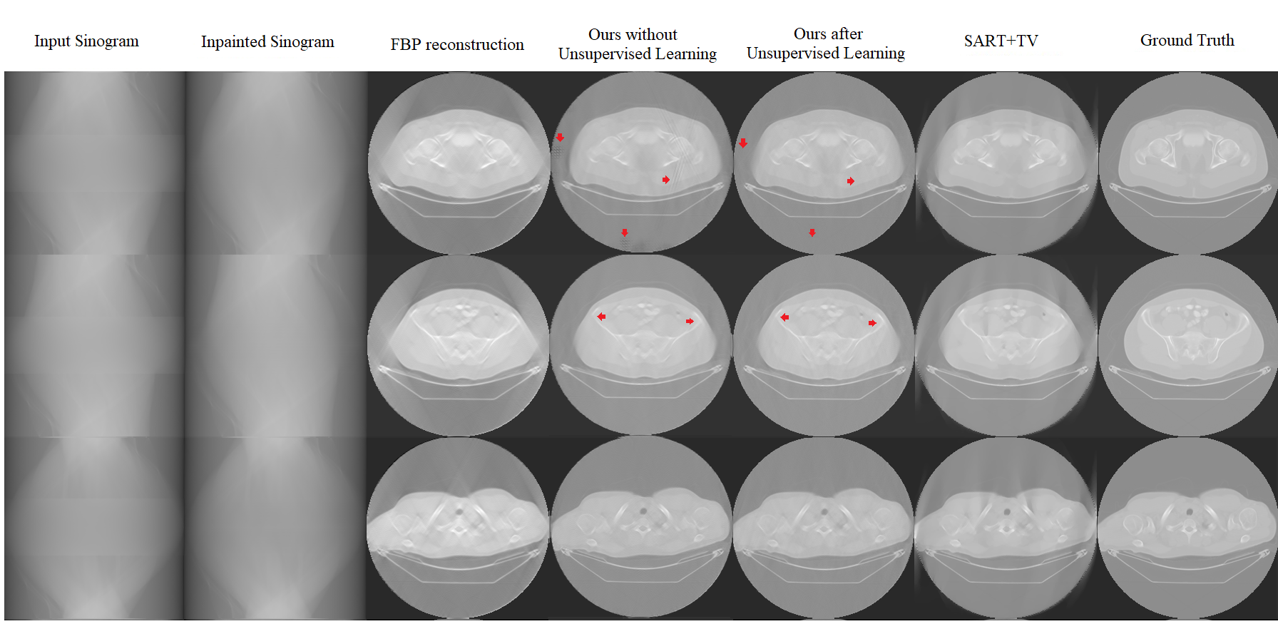
Figure 10: The inpainted sinogram and reconstructed images for test datasets of Zubal’s phantom. We compare three reconstruction methods: FBP, our proposed supervised-trained network before/after 30-epochs unsupervised learning, and iterative SART reconstruction with TV regularization. The results indicate the effects of unsupervised train, which consist of eliminating the artifacts introduced by overfitting (row1) and making the edges in image slightly sharper (row2). And the data fidelity implied in loss ensures the image quality not to degrade in training (row3). The display window is [-1, 1].

TABLE II: Quantitative Comparsion for FBP, SART-TV and Proposed Method for Zubal CT dataset (40 slices)

	FBP	SART-TV	Proposed
avg. PSNR(dB)	24.88	28.08	36.33
avg. SSIM	0.9598	0.9523	0.9838

IV Conclusions

In this paper we designed a network architecture with a deep convolutional network SIN for sinogram inpainting task, new-designed differentiable Radon/Inverse Radon Transformer modules for cross-domain error backward-propagation and image processing network for eliminating artifacts. Though we focused on limited angle task, the proposed sinogram inpainting method can also be used in metal artifact reduction.

This approach can be trained both supervisedly and unsupervisedly to tackle the labeled data bottleneck. In supervised training, our method can join both sinogram and reconstruction error in the loss and optimize in sync with data fidelity, thanks to the differentiable radon transformer. In unsupervised training, we design a closed loop and use the inconsistence in closed loop as loss function, so we can train on only limited-angle sinogram while satisfying data-fidelity.

The proposed method performs better than state-of-art iterative reconstruction SART-TV at different body positions, covering both supervisedly and unsupervisedly learned ones. Furthermore, free from difficulty in selecting superparameters and iterative projections/backprojections in SART, the reconstruction time of our proposed network can be less than 0.3 second per 256*256 image in parallel batches.

V Appendix

For someone that is interested in implementation in our proposed method, we attach an architecture figure of modified pix2pix network for sinogram inpainting network. And the pix2pix network in image processing network shares the same architecture.

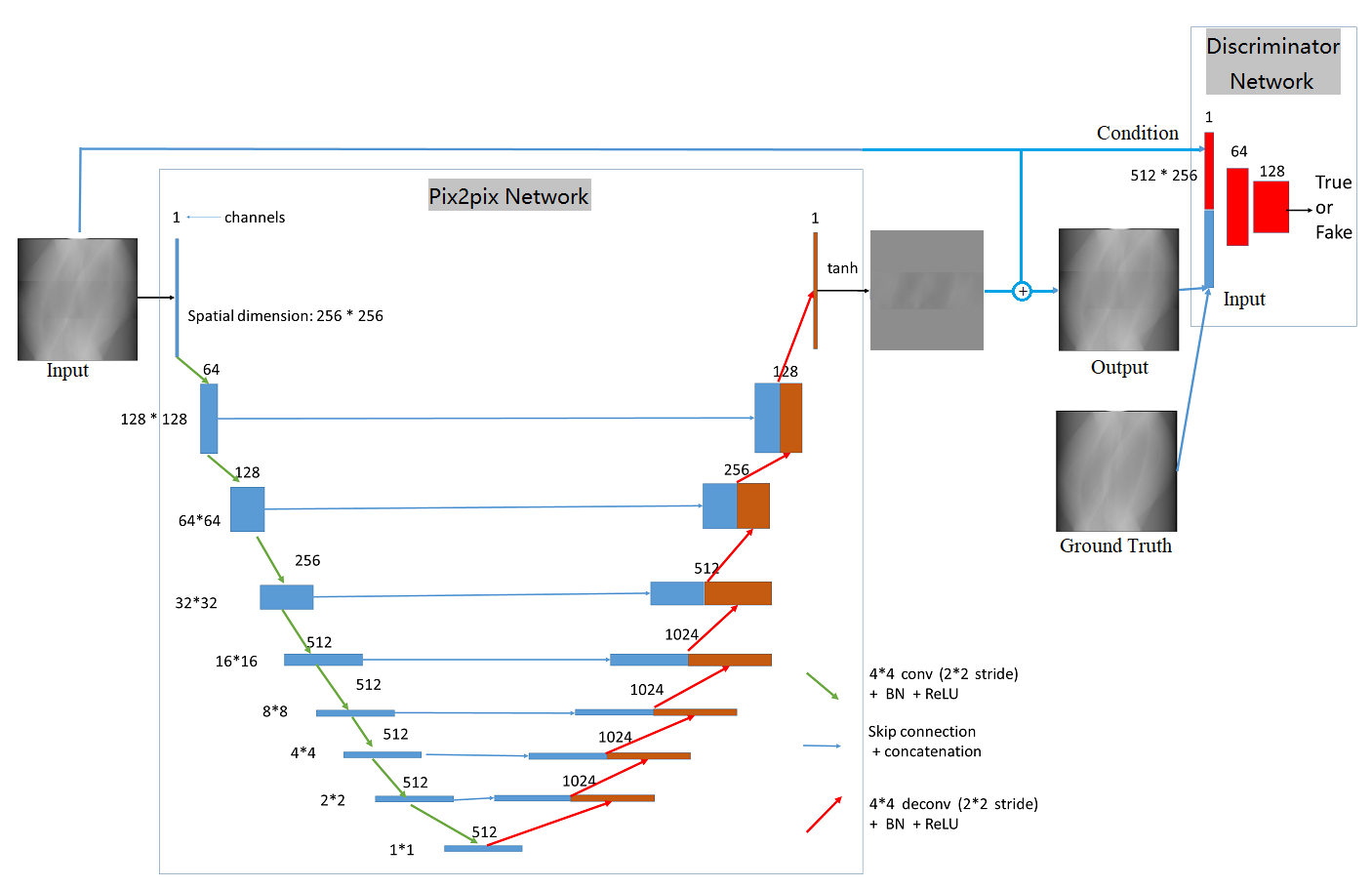
Figure 11: Architecture of the proposed deep convolutional network based on pix2pix network except using the scanning data to replace corresponding part in fake images, which forces the $G_{s}$ focusing on learning the missing part.

References

- [1] Y. Zhang, H.-P. Chan, B. Sahiner, J. Wei, M. M. Goodsitt, L. M. Hadjiiski, J. Ge, and C. Zhou, “A comparative study of limited-angle cone-beam reconstruction methods for breast tomosynthesis,” Medical physics, vol. 33, no. 10, pp. 3781–3795, 2006.
- [2] M. Rantala, S. Vanska, S. Jarvenpaa, M. Kalke, M. Lassas, J. Moberg, and S. Siltanen, “Wavelet-based reconstruction for limited-angle x-ray tomography,” IEEE transactions on medical imaging, vol. 25, no. 2, pp. 210–217, 2006.
- [3] X. Jin, L. Li, Z. Chen, L. Zhang, and Y. Xing, “Motion-compensated reconstruction method based on rigid motion model with multi-object,” Tsinghua Science & Technology, vol. 15, no. 1, pp. 120–126, 2010.
- [4] Y. Ye, H. Yu, and G. Wang, “Exact interior reconstruction from truncated limited-angle projection data,” Journal of Biomedical Imaging, vol. 2008, p. 5, 2008.
- [5] E. J. Candès, J. Romberg, and T. Tao, “Robust uncertainty principles: Exact signal reconstruction from highly incomplete frequency information,” IEEE Transactions on information theory, vol. 52, no. 2, pp. 489–509, 2006.
- [6] R. Gordon, R. Bender, and G. T. Herman, “Algebraic reconstruction techniques (art) for three-dimensional electron microscopy and x-ray photography,” Journal of theoretical Biology, vol. 29, no. 3, pp. 471IN1477–476IN2481, 1970.
- [7] E. J. Candes and J. K. Romberg, “Signal recovery from random projections.” Computational Imaging, vol. 3, pp. 76–86, 2005.
- [8] H. Yu and G. Wang, “Compressed sensing based interior tomography,” Physics in Medicine and Biology, vol. 54, no. 9, p. 2791, 2009. [Online]. Available: http://stacks.iop.org/0031-9155/54/i=9/a=014
- [9] Z. Chen, X. Jin, L. Li, and G. Wang, “A limited-angle ct reconstruction method based on anisotropic tv minimization,” Physics in medicine and biology, vol. 58, no. 7, p. 2119, 2013.
- [10] A. Mehranian, M. Ay, A. Rahmim, and H. Zaidi, “Sparsity constrained sinogram inpainting for metal artifact reduction in x-ray computed tomography,” in Nuclear Science Symposium and Medical Imaging Conference (NSS/MIC), 2011 IEEE. IEEE, 2011, pp. 3694–3699.
- [11] Y. Chen, Y. Li, H. Guo, Y. Hu, L. Luo, X. Yin, J. Gu, and C. Toumoulin, “Ct metal artifact reduction method based on improved image segmentation and sinogram in-painting,” Mathematical Problems in Engineering, vol. 2012, 2012.
- [12] C. Peng, B. Qiu, M. Li, Y. Guan, C. Zhang, Z. Wu, and J. Zheng, “Gaussian diffusion sinogram inpainting for x-ray ct metal artifact reduction,” Biomedical engineering online, vol. 16, no. 1, p. 1, 2017.
- [13] Y. Kim, S. Yoon, and J. Yi, “Effective sinogram-inpainting for metal artifacts reduction in x-ray ct images,” in Image Processing (ICIP), 2010 17th IEEE International Conference on. IEEE, 2010, pp. 597–600.
- [14] S. Li, Q. Cao, Y. Chen, Y. Hu, L. Luo, and C. Toumoulin, “Dictionary learning based sinogram inpainting for ct sparse reconstruction,” Optik-International Journal for Light and Electron Optics, vol. 125, no. 12, pp. 2862–2867, 2014.
- [15] Y. Li, Y. Chen, Y. Hu, A. Oukili, L. Luo, W. Chen, and C. Toumoulin, “Strategy of computed tomography sinogram inpainting based on sinusoid-like curve decomposition and eigenvector-guided interpolation,” JOSA A, vol. 29, no. 1, pp. 153–163, 2012.
- [16] H. Gao, Y. Xing, L. Zhang, Z. Chen, and J. Cheng, “Fast and robust edge-preserving image reconstruction for limited-angle tomography,” in The 9th International Meeting on Fully Three Dimensional Image Reconstruction in Radiology and Nuclear Medicine, 2007.
- [17] Y. LeCun, Y. Bengio, and G. Hinton, “Deep learning,” Nature, vol. 521, no. 7553, pp. 436–444, 2015.
- [18] K. He, X. Zhang, S. Ren, and J. Sun, “Deep residual learning for image recognition,” in Proceedings of the IEEE conference on computer vision and pattern recognition, 2016, pp. 770–778.
- [19] C. Szegedy, S. Ioffe, V. Vanhoucke, and A. A. Alemi, “Inception-v4, inception-resnet and the impact of residual connections on learning.” in AAAI, 2017, pp. 4278–4284.
- [20] J. Redmon, S. Divvala, R. Girshick, and A. Farhadi, “You only look once: Unified, real-time object detection,” in Proceedings of the IEEE Conference on Computer Vision and Pattern Recognition, 2016, pp. 779–788.
- [21] R. Girshick, “Fast r-cnn,” in Proceedings of the IEEE international conference on computer vision, 2015, pp. 1440–1448.
- [22] S. Ren, K. He, R. Girshick, and J. Sun, “Faster r-cnn: Towards real-time object detection with region proposal networks,” in Advances in neural information processing systems, 2015, pp. 91–99.
- [23] J. Kim, J. Kwon Lee, and K. Mu Lee, “Accurate image super-resolution using very deep convolutional networks,” in Proceedings of the IEEE Conference on Computer Vision and Pattern Recognition, 2016, pp. 1646–1654.
- [24] C. Ledig, L. Theis, F. Huszár, J. Caballero, A. Cunningham, A. Acosta, A. Aitken, A. Tejani, J. Totz, Z. Wang et al., “Photo-realistic single image super-resolution using a generative adversarial network,” arXiv preprint arXiv:1609.04802, 2016.
- [25] D. Pathak, P. Krahenbuhl, J. Donahue, T. Darrell, and A. A. Efros, “Context encoders: Feature learning by inpainting,” in Proceedings of the IEEE Conference on Computer Vision and Pattern Recognition, 2016, pp. 2536–2544.
- [26] Q. Xu, H. Yu, X. Mou, L. Zhang, J. Hsieh, and G. Wang, “Low-dose x-ray ct reconstruction via dictionary learning,” IEEE Transactions on Medical Imaging, vol. 31, no. 9, pp. 1682–1697, 2012.
- [27] H. Zhang, L. Li, K. Qiao, L. Wang, B. Yan, L. Li, and G. Hu, “Image prediction for limited-angle tomography via deep learning with convolutional neural network,” arXiv preprint arXiv:1607.08707, 2016.
- [28] K. H. Jin, M. T. McCann, E. Froustey, and M. Unser, “Deep convolutional neural network for inverse problems in imaging,” IEEE Transactions on Image Processing, 2017.
- [29] O. Ronneberger, P. Fischer, and T. Brox, “U-net: Convolutional networks for biomedical image segmentation,” in International Conference on Medical Image Computing and Computer-Assisted Intervention. Springer, 2015, pp. 234–241.
- [30] G. Wang, “A perspective on deep imaging,” IEEE Access, vol. 4, pp. 8914–8924, 2016.
- [31] H. Chen, Y. Zhang, M. K. Kalra, F. Lin, P. Liao, J. Zhou, and G. Wang, “Low-dose ct with a residual encoder-decoder convolutional neural network (red-cnn),” arXiv preprint arXiv:1702.00288, 2017.
- [32] B. C. Csáji, “Approximation with artificial neural networks,” Faculty of Sciences, Etvs Lornd University, Hungary, vol. 24, p. 48, 2001.
- [33] I. G. Zubal, C. R. Harrell, E. O. Smith, Z. Rattner, G. Gindi, and P. B. Hoffer, “Computerized three-dimensional segmented human anatomy,” Medical physics, vol. 21, no. 2, pp. 299–302, 1994.
- [34] F. Noo, R. Clackdoyle, and J. D. Pack, “A two-step hilbert transform method for 2d image reconstruction,” Physics in Medicine and Biology, vol. 49, no. 17, p. 3903, 2004.
- [35] J. D. Pack, F. Noo, and R. Clackdoyle, “Cone-beam reconstruction using the backprojection of locally filtered projections,” IEEE Transactions on Medical Imaging, vol. 24, no. 1, pp. 70–85, 2005.
- [36] P. Isola, J. Zhu, T. Zhou, and A. A. Efros, “Image-to-image translation with conditional adversarial networks,” CoRR, vol. abs/1611.07004, 2016. [Online]. Available: http://arxiv.org/abs/1611.07004
- [37] M. Jaderberg, K. Simonyan, A. Zisserman et al., “Spatial transformer networks,” in Advances in Neural Information Processing Systems, 2015, pp. 2017–2025.
- [38] D. He, Y. Xia, T. Qin, L. Wang, N. Yu, T. Liu, and W.-Y. Ma, “Dual learning for machine translation,” in Advances in Neural Information Processing Systems, 2016, pp. 820–828.