Delta-map method to remove CMB foregrounds with spatially varying spectra

Abstract

We extend the internal template foreground removal method by accounting for spatially varying spectral parameters such as the spectral indices of synchrotron and dust emission and the dust temperature. As the previous algorithm had to assume that the spectral parameters are uniform over the full sky (or some significant fraction of the sky), it resulted in a bias in the tensor-to-scalar ratio parameter $r$ estimated from foreground-cleaned polarization maps of the cosmic microwave background (CMB). The new algorithm, “Delta-map method”, accounts for spatially varying spectra to first order in perturbation. The only free parameters are the cosmological parameters such as $r$ and the sky-averaged foreground parameters. We show that a cleaned CMB map is the maximum likelihood solution to first order in perturbation, and derive the posterior distribution of $r$ and the sky-averaged foreground parameters using Bayesian statistics. Applying this to realistic simulated sky maps including polarized CMB, synchrotron and thermal dust emission, we find that the new algorithm removes the bias in $r$ down to undetected level in our noiseless simulation ($r\lesssim 4\times 10^{-4}$). We show that the frequency decorrelation of polarized foregrounds due to averaging of spatially varying spectra can be accounted for to first order in perturbation by using slightly different spectral parameters for the Stokes $Q$ and $U$ maps. Finally, we show that the effect of polarized anomalous microwave emission on foreground removal can be absorbed into the curvature parameter of the synchrotron spectrum.

xxxx, xxx

1 Introduction

Search for the signature of primordial gravitational waves from the early Universe in the B-mode polarization of the cosmic microwave background (CMB) 2016ARAA..54..227K is limited already by accuracy of the foreground removal procedure 2015PhRvL.114j1301B . Among various methods for removing the foreground emission (see 2008A&A…491..597L ; 2018JCAP…04..023R ; 2018arXiv180706208P and references therein), we focus on the so-called “internal template” method 2007ApJS..170..335P ; 2009MNRAS.397.1355E ; 2011ApJ…737…78K ; 2012MNRAS.420.2162F ; 2016MNRAS.459..441F . The basic idea behind this method is simple. Consider that we have maps at three frequencies: low, middle, and high. Say 40, 100, and 240 GHz. We know that the low and high frequency data are dominated by synchrotron and thermal dust emission, respectively 2014PTEP.2014fB109I ; thus, the simplest way to remove them is to fit the low- and high-frequency maps to and subtract from the map at the middle frequency. A cleaned map may be written as $x=([Q,U]_{100}+\alpha_{40}[Q,U]_{40}+\alpha_{240}[Q,U]_{240})/(1+\alpha_{40}+\alpha_{240})$, where $\alpha_{40}$ and $\alpha_{240}$ are fitting coefficients and $Q$ and $U$ are the Stokes parameters in thermodynamic temperature units. Fitting can be done in pixel, Fourier (spherical harmonics), or wavelet space. This method is called a template because the low and high frequency data are used as templates of synchrotron and thermal dust emission, respectively, and is called internal because no external data sets are used.

All of the previous implementations of this method assumed that the fitting coefficients are uniform over some fitted regions. In some study the fitted region was taken to be the whole sky 2007ApJS..170..335P ; 2009MNRAS.397.1355E ; 2012MNRAS.420.2162F ; 2016MNRAS.459..441F , whereas in the other some large pixels 2011ApJ…737…78K . In this paper, we build on our previous work 2011ApJ…737…78K , in which we find that the internal template method yields a small but non-negligible bias in the tensor-to-scalar ratio parameter $r$ of order $10^{-3}$, and that the origin of the bias is the spatial variation of the fitting coefficients, i.e., spatial variation of the spectral parameters of the foreground emission.

Motivated by this finding, we extend the internal template method by accounting for spatial variations of the spectra. If we have two high (or low) frequency channels as dust (or synchrotron) templates instead of one, we should be able to solve for both the mean and variation in one spectral parameter, e.g., the dust (or synchrotron) spectral index. We show that this is indeed the case. In general, we need $N+1$ channels to account for spatial variations of $N$ spectral parameters of one foreground component.

Armed with the new method, which we shall call the “Delta-map method” throughout this paper, we investigate two hotly debated topics of the polarized foreground: treatments of possible polarization in the anomalous microwave emission (AME) and the frequency decorrelation due to averaging of spatially varying foreground spectra.

This paper is organized as follows. We introduce the Delta-map method in Sect. 2, and explain how to implement it in Sect. 3. In Sect. 4, we interpret the Delta-map method within the Bayesian framework. In Sect. 5, we apply this to realistic foreground maps for validation. In Sect. 6, we show how to treat AME and frequency decorrelation. In Sect. 7, we study how instrumental noise affects the results. We conclude in Sect. 8.

2 Delta-map method

2.1 General formula

Without loss of generality, let us consider one foreground component with $N$ spectral parameters, and model the observed Stokes parameters $Q$ and $U$ in thermodynamic temperature units at a given frequency $\nu$ as

$$[Q,U]_{\nu}(\hat{n})=\mbox{CMB}(\hat{n})+g_{\nu}D_{\nu}(p^{I}(\hat{n}))[Q^{f},U^{f}]_{\nu_{\ast}}(\hat{n})+N_{\nu}(\hat{n})~{},$$ (1)

where $\mbox{CMB}(\hat{n})$ and $N_{\nu}(\hat{n})$ denote the CMB signal and instrumental noise towards a sky direction $\hat{n}$ in thermodynamic units, respectively, and $[Q^{f},U^{f}]_{\nu_{\ast}}(\hat{n})$ denotes the foreground component at some reference frequency $\nu_{\ast}$ in brightness temperature units. As the dependence on $\nu_{*}$ cancels in the final result, $[Q^{f},U^{f}]_{\nu_{\ast}}$ appears only as an auxiliary variable. For simplicity we have not written explicitly experiment-specific effects such as a gain calibration factor, beam smearing, pixel window function, or any other smoothing/filtering that may be applied to data. Such operations will be common to all sky signals at the same frequency channel.

The coefficient $g_{\nu}$ is given by

$$g_{\nu}\equiv\frac{(e^{x}-1)^{2}}{e^{x}x^{2}}~{}~{}\mbox{with}~{}~{}x\equiv\frac{h\nu}{k_{B}T_{\rm CMB}}~{},$$ (2)

which converts the units from brightness temperature to the CMB thermodynamic temperature ($T_{\rm CMB}=2.725$ K). While this expression does not take into account averaging over the bandpass of detectors, we shall include it in Sect. 2.5.

The function $D_{\nu}$ denotes the frequency dependence of the foreground emission in brightness temperature units, and $p^{I}(\hat{n})$ a set of parameters ($I=1,2,\cdots,N$) that characterize the emission law and can vary across the sky. For example, if we consider a power-law foreground emission component, then $N=1$ and $p^{1}(\hat{n})$ is a power-law spectral index $\beta(\hat{n})$. Thus, $D_{\nu}=\left({\nu}/{\nu_{\ast}}\right)^{\beta(\hat{n})}$. Decomposing the spectral parameters to the mean value and perturbation as $p^{I}(\hat{n})=\bar{p}^{I}+\delta p^{I}(\hat{n})$, we obtain

$$D_{\nu}(p^{I}(\hat{n}))[Q^{f},U^{f}]_{\nu_{\ast}}(\hat{n})=D_{\nu}(\bar{p}^{I})[Q^{f},U^{f}]_{\nu_{\ast}}(\hat{n})+\sum_{J=1}^{N}D_{\nu,J}\delta p^{J}(\hat{n})[Q^{f},U^{f}]_{\nu_{\ast}}(\hat{n})+{\cal O}(\delta p^{2})\,,$$ (3)

where we wrote $D_{\nu,J}\equiv\left({\partial D_{\nu}}/{\partial p^{J}}\right)_{p^{J}=\bar{p}^{J}}$.

The central assumption we make throughout this paper is that we truncate the expansion at first order in $\delta p^{I}$ 1999NewA….4..443B ; 2016ApJ…829..113S . Therefore, when a foreground component is parameterized by $N$ parameters that vary across the sky only weakly, we can interpret the emission as a superposition of $(N+1)$ template maps; namely $[Q^{f},U^{f}]_{\nu_{\ast}}(\hat{n})$ and $\delta p^{I}(\hat{n})[Q^{f},U^{f}]_{\nu_{\ast}}(\hat{n})$ $(I=1,2,\cdots,N)$. If the ${\cal O}(\delta p^{2})$ term is significant compared with the first two terms, it may cause a bias in $r$ as foreground residuals. The bias becomes greater when the foreground channels are taken further away from the CMB channel. We find, however, that the bias is negligible for the band specification and realistic simulated sky maps used in this work, as we shall show later.

To subtract the foreground component in Eq. (1) with help of Eq. (3), we form a linear combination of $(N+2)$ maps at different frequencies as

$$[Q,U]_{\nu_{\rm CMB}}(\hat{n})+\sum_{j=1}^{N+1}\alpha_{j}[Q,U]_{\nu_{j}}(\hat{n}) = \left(1+\sum_{j=1}^{N+1}\alpha_{j}\right)\mbox{CMB}(\hat{n})$$ (4)

$$+ \left(g_{\nu_{\rm CMB}}D_{\nu_{\rm CMB}}(\bar{p}^{I})+\sum_{j=1}^{N+1}\alpha_{j}g_{\nu_{j}}D_{\nu_{j}}(\bar{p}^{I})\right)[Q^{f},U^{f}]_{\nu_{\ast}}(\hat{n})$$

$$+ \sum_{J=1}^{N}\left(g_{\nu_{\rm CMB}}D_{\nu_{\rm CMB},J}+\sum_{j=1}^{N+1}\alpha_{j}g_{\nu_{j}}D_{\nu_{j},J}\right)\delta p^{J}(\hat{n})[Q^{f},U^{f}]_{\nu_{\ast}}(\hat{n})$$

$$+ N_{\nu_{\rm CMB}}(\hat{n})+\sum_{j=1}^{N+1}\alpha_{j}N_{\nu_{j}}(\hat{n})~{},$$

where $\alpha_{j}$ are fitting coefficients, $\nu_{\rm CMB}$ denotes a frequency employed as a CMB channel, and $\nu_{j}$ the foreground channels. The fitting coefficients are found by setting the foreground terms in the above equation (i.e., the second and third lines) to zero:

$$g_{\nu_{\rm CMB}}D_{\nu_{\rm CMB}}(\bar{p}^{I})+\sum_{j=1}^{N+1}g_{\nu_{j}}D_{\nu_{j}}(\bar{p}^{I})\alpha_{j} = 0\,,$$ (5)

$$g_{\nu_{\rm CMB}}D_{\nu_{\rm CMB},J}+\sum_{j=1}^{N+1}g_{\nu_{j}}D_{{\nu_{j}},J}\alpha_{j} = 0\,,\quad\mbox{for}~{}J=(1,2,\cdots,N).$$ (6)

These equations can be cast into a matrix form as ${\bm{A}}\vec{\alpha}=-\vec{d}_{\nu_{\rm CMB}}$, where

$$\vec{\alpha} \equiv (\alpha_{1},\alpha_{2},\cdots,\alpha_{N+1})^{\rm T}~{},$$ (7)

$$\vec{d}_{\nu} \equiv g_{\nu}\left(D_{\nu}(\bar{p}^{I}),D_{\nu,1},\cdots,D_{\nu,N}\right)^{\rm T}~{},$$ (8)

$${\bm{A}} \equiv (\vec{d}_{\nu_{1}},\vec{d}_{\nu_{2}},\cdots,\vec{d}_{\nu_{N+1}})~{}.$$ (9)

The coefficients $\alpha_{j}$ can be obtained numerically by $-{\bm{A}}^{-1}\vec{d}_{\nu_{\rm CMB}}$. Once the coefficients are determined, we obtain a foreground-cleaned CMB map $\vec{x}$ as

$$\vec{x}=\frac{[Q,U]_{\nu_{\rm CMB}}(\hat{n})+\sum_{j=1}^{N+1}\alpha_{j}[Q,U]_{\nu_{j}}(\hat{n})}{1+\sum_{j=1}^{N+1}\alpha_{j}}\,.$$ (11)

Since this is a linear combination of maps, we can construct a cleaned CMB in pixel, spherical harmonics, or wavelet space.

Multi-component foregrounds can be incorporated straightforwardly by expanding the entries of ${\bm{A}}$. For example, if we use $D_{\nu}$ for dust and $S_{\nu}$ for synchrotron, we may define a new vector for synchrotron as

$$\vec{s}_{\nu}\equiv g_{\nu}\left(S_{\nu}(\bar{p}^{J}),S_{\nu,1},\cdots,S_{\nu,M}\right)^{\rm T}~{},$$ (12)

where $M$ is the number of parameters characterizing synchrotron, and write the matrix $\bm{A}$ as

$${\bm{A}}=(\vec{d}_{\nu_{1}},\vec{d}_{\nu_{2}},\cdots,\vec{d}_{\nu_{N+1}},\vec{s}_{\nu_{1}},\vec{s}_{\nu_{2}},\cdots,\vec{s}_{\nu_{M+1}})~{}.$$ (13)

There are $N+M+2$ coefficients to be determined, and are given by $\vec{\alpha}=-\bm{A}^{-1}(\vec{d}_{\nu_{\rm CMB}},\vec{s}_{\nu_{\rm CMB}})^{\rm T}$. Thus, obtaining one cleaned CMB map requires at least $N+M+3$ frequencies. In Sect. 4, we derive the formula for a cleaned CMB map when we have more frequency channels than this minimum number.

2.2 Power law

To obtain a better feel for the new algorithm, let us work out three simpler, concrete examples.

First, we consider a single power-law spectrum with a spatially varying spectral index:

$$D_{\nu}(p^{I}(\hat{n}))=D_{\nu}(\beta(\hat{n}))=\left(\frac{\nu}{\nu_{\ast}}\right)^{\beta(\hat{n})}~{}.$$ (14)

The Stokes parameters become 1999NewA….4..443B ; 2016ApJ…829..113S

$$[Q,U]_{\nu}(\hat{n})=\mbox{CMB}(\hat{n})+N_{\nu}(\hat{n})+g_{\nu}\left(\frac{\nu}{\nu_{\ast}}\right)^{\bar{\beta}}\left(1+\ln\left(\frac{\nu}{\nu_{\ast}}\right)\delta\beta(\hat{n})\right)[Q^{f},U^{f}]_{\nu_{\ast}}(\hat{n})+{\cal O}(\delta p^{2})~{},$$ (15)

where $\bar{\beta}$ is the mean spectral index. Eq. (8) becomes

$$\vec{d}_{\nu}=g_{\nu}\left(\frac{\nu}{\nu_{\ast}}\right)^{\bar{\beta}}\left(1,\ln\left(\frac{\nu}{\nu_{\ast}}\right)\right)^{\rm T}~{}.$$ (16)

Therefore, the sum in Eq. (11) evaluates to

$$\sum_{j=1}^{2}\alpha_{j}\left[Q,U\right]_{\nu_{j}}(\hat{n})=\frac{g_{\nu_{\rm CMB}}}{\ln(\nu_{2}/\nu_{1})} \left\{\frac{1}{g_{\nu_{2}}}\left(\frac{\nu_{\rm CMB}}{\nu_{2}}\right)^{\bar{\beta}}\ln(\nu_{1}/\nu_{\rm CMB})[Q,U]_{\nu_{2}}(\hat{n})\right.$$

$$-\left.\frac{1}{g_{\nu_{1}}}\left(\frac{\nu_{\rm CMB}}{\nu_{1}}\right)^{\bar{\beta}}\ln(\nu_{2}/\nu_{\rm CMB})[Q,U]_{\nu_{1}}(\hat{n})\right\}\,.$$ (17)

The reference frequency $\nu_{*}$ cancels in the final result, which is required from the physical ground: a cleaned CMB map result should be invariant under an arbitrary change in the reference frequency. Adding this to $[Q,U]_{\nu_{\rm CMB}}(\hat{n})$ removes the foreground emission including spatial variation of the spectral index to first order in $\delta\beta(\hat{n})$. Note that we do not fit for $\delta\beta$ because they are solved and eliminated. The only fitting parameter is the mean spectral index $\bar{\beta}$.

As the above expression uses a difference between two weighted maps at different frequencies, we started to call this map a “Delta-map”, which became the name of our algorithm. However, as we show in Sect. 4, our algorithm is much more general than Eq. (17). A more appropriate (and general) reason for the name “Delta-map” would be the fact that we expand and truncate the spectral dependence of foregrounds at first order in perturbation. Henceforth we shall adopt this reasoning for the name of the algorithm.

2.3 Running spectral index

Second, we allow the spectral index to vary slowly with frequency:

$$D_{\nu}(p^{I}(\hat{n}))=D_{\nu}(\beta(\hat{n}),C(\hat{n}))=\left(\frac{\nu}{\nu_{*}}\right)^{\beta(\hat{n})+C(\hat{n})\ln\left({\nu}/{\nu_{\rm s}}\right)}~{},$$ (18)

where ${C}$ is the so-called curvature parameter or running of the spectral index, $\bar{C}$ is its mean value, and $\nu_{\rm s}$ is a pivot frequency of running index. There is no physical meaning for $\nu_{\rm s}$, but it can be chosen such that it minimizes a correlation between $\beta$ and $C$.

The Stokes parameters become

$$[Q,U]_{\nu}(\hat{n}) = \mbox{CMB}(\hat{n})+N_{\nu}(\hat{n})$$ (19)

$$+ g_{\nu}\left(\frac{\nu}{\nu_{*}}\right)^{\bar{\beta}+\bar{C}\ln\left({\nu}/{\nu_{\rm s}}\right)}\left[1+\ln\left(\frac{\nu}{\nu_{*}}\right)\left(\delta\beta(\hat{n})+\ln\left(\frac{\nu}{\nu_{\rm s}}\right)\delta C(\hat{n})\right)\right][Q^{f},U^{f}]_{\nu_{*}}(\hat{n})$$

$$+ {\cal O}(\delta p^{2})\,,$$

and

$${\vec{d}}_{\nu}=g_{\nu}\left(\frac{\nu}{\nu_{*}}\right)^{\bar{\beta}+\bar{C}\ln\left({\nu}/{\nu_{\rm s}}\right)}\left(1,\ln\left(\frac{\nu}{\nu_{*}}\right),\ln\left(\frac{\nu}{\nu_{*}}\right)\ln\left(\frac{\nu}{\nu_{\rm s}}\right)\right)^{\rm T}$$ (20)

In this case, we need maps at three different frequencies to remove the effects of spatially varying foreground parameters to first order in $\delta\beta(\hat{n})$ and $\delta C(\hat{n})$.

2.4 Modified Blackbody

Finally, we consider a modified blackbody (MBB) spectrum for dust emission:

$$D_{\nu}(p^{I}(\hat{n}))=D_{\nu}(\beta_{\rm d}(\hat{n}),T_{\rm d}(\hat{n}))=\left(\frac{\nu}{\nu_{*}}\right)^{\beta_{\rm d}(\hat{n})+1}\frac{e^{x_{{\rm d}*}(\hat{n})}-1}{e^{x_{\rm d}(\hat{n})}-1}~{},$$ (21)

where $x_{\rm d}(\hat{n})\equiv h\nu/k_{B}T_{\rm d}(\hat{n})$, $x_{{\rm d}*}(\hat{n})\equiv h\nu_{*}/k_{B}T_{\rm d}(\hat{n})$, and $T_{\rm d}(\hat{n})$ is the dust temperature. In the low-frequency limit, $D_{\nu}\to(\nu/\nu_{*})^{\beta_{\rm d}}$. The Stokes parameters become

$$[Q,U]_{\nu}(\hat{n}) = \mbox{CMB}(\hat{n})+N_{\nu}(\hat{n})+g_{\nu}\left(\frac{\nu}{\nu_{*}}\right)^{\bar{\beta}_{\rm d}+1}\frac{e^{\bar{x}_{{\rm d}*}-1}}{e^{\bar{x}_{\rm d}}-1}$$ (22)

$$\times\left[1+\ln\left(\frac{\nu}{\nu_{*}}\right)\delta\beta_{\rm d}(\hat{n})+\left(\frac{\bar{x}_{\rm d}e^{\bar{x}_{\rm d}}}{e^{\bar{x}_{\rm d}}-1}-\frac{\bar{x}_{{\rm d}*}e^{\bar{x}_{{\rm d}*}}}{e^{\bar{x}_{{\rm d}*}}-1}\right)\frac{\delta T_{\rm d}(\hat{n})}{\bar{T_{\rm d}}}\right][Q^{f},U^{f}]_{\nu_{*}}(\hat{n})$$

$$+ {\cal O}(\delta p^{2})\,,$$

where $\bar{T}_{\rm d}$ is the mean temperature, $\bar{x}_{\rm d}\equiv h\nu/k\bar{T}_{\rm d}$, and

$${\vec{d}}_{\nu}=g_{\nu}\left(\frac{\nu}{\nu_{*}}\right)^{\bar{\beta}_{\rm d}+1}\frac{e^{\bar{x}_{{\rm d}*}}-1}{e^{\bar{x}_{\rm d}}-1}\left(1,\ln\left(\frac{\nu}{\nu_{*}}\right),\left(\frac{\bar{x}_{\rm d}e^{\bar{x}_{\rm d}}}{e^{\bar{x}_{\rm d}}-1}-\frac{\bar{x}_{{\rm d}*}e^{\bar{x}_{{\rm d}*}}}{e^{\bar{x}_{{\rm d}*}}-1}\right)\frac{1}{\bar{T}_{\rm d}}\right)^{\rm T}~{}.$$ (23)

In this case, we need maps at three different frequencies to remove the effects of spatially varying foreground parameters to first order in $\delta\beta_{\rm d}(\hat{n})$ and $\delta T_{\rm d}(\hat{n})$.

2.5 Bandpass average

The above formalism applies when we have detectors with a delta-function response to a single frequency. In reality the sky signal must be averaged within a given bandpass of detectors.

To incorporate the bandpass average, we first average an observed intensity as

$$\left<I(\nu)\right>\equiv\frac{\int W(\nu^{\prime})I(\nu^{\prime})d\nu^{\prime}}{\int W(\nu^{\prime})d\nu^{\prime}}=\frac{1}{\Delta\nu}\int_{\nu-\Delta\nu/2}^{\nu+\Delta\nu/2}I(\nu^{\prime})d\nu^{\prime}~{},$$ (24)

where the last equality holds when the bandpass function $W(\nu)$ is a top hat function with a width of $\Delta\nu$. We then relate $\left<I(\nu)\right>$ to the thermodynamic CMB temperature fluctuation $\delta T$ as

$$\left<I(\nu)\right>=\left<\frac{\partial B_{\nu}(T)}{\partial T}\right>\delta T~{},$$ (25)

where $B_{\nu}(T)$ is a blackbody intensity spectrum. The same relation holds for the Stokes parameters $Q$ and $U$.

We use the brightness temperature as an intermediate step between the intensity and thermodynamic temperature. The brightness-thermodynamic temperature conversion factor $g_{\nu}$ (Eq. 2) with bandpass averaging is then given by

$$\left<g_{\nu}\right>=\frac{2k_{B}\nu^{2}/c^{2}}{\left<\frac{\partial B_{\nu}(T)}{\partial T}\right>}=\frac{\nu^{2}}{\left<\nu^{2}\frac{e^{x}x^{2}}{(e^{x}-1)^{2}}\right>}~{}.$$ (26)

There is no averaging for $\nu^{2}$ in the numerator because it is the intensity that is averaged, and conversion from the intensity to brightness temperature is merely an intermediate step. Using these quantities, our sky model (Eq. (1)) is now expressed as

$$[Q,U]_{\nu}(\hat{n}) = \mbox{CMB}(\hat{n})+\left<g_{\nu}\right>\frac{\left<\nu^{2}D_{\nu}(p^{I}(\hat{n}))\right>}{\nu^{2}}[Q^{f},U^{f}]_{\nu_{\ast}}(\hat{n})+N_{\nu}(\hat{n})$$ (27)

$$= \mbox{CMB}(\hat{n})+\frac{\left<\nu^{2}D_{\nu}(p^{I}(\hat{n}))\right>}{\left<\nu^{2}\frac{e^{x}x^{2}}{(e^{x}-1)^{2}}\right>}[Q^{f},U^{f}]_{\nu_{\ast}}(\hat{n})+N_{\nu}(\hat{n})\,.$$

As $[Q^{f},U^{f}]_{\nu_{\ast}}$ is an auxiliary variable, there is no need to bandpass-average it. The average is done only for variables depending on $\nu$. Therefore, to incorporate bandpass averaging, all we need is to replace $g_{\nu}D_{\nu}$ with $\langle g_{\nu}\rangle\langle\nu^{2}D_{\nu}\rangle/\nu^{2}$.

Incorporating bandpass averaging in the foreground removal algorithm is important because it changes the effective frequency at which intensity of foregrounds should be evaluated. Using an incorrect bandpass leads to a bias in $r$. How precisely we should know the bandpass needs to be determined by the requirement for science, e.g., a target value of $r$, coupled with a careful analysis including foreground removal and systematic errors in our knowledge of the bandpass. This is work in progress. For the rest of this paper we shall ignore bandpass averaging in the simulations and leave detailed study of its effect for future work.

3 Implementation

3.1 Cleaning one map

Our likelihood for a cleaned CMB map $\vec{x}$ (Eq. (11)) is

$$-2\ln{\cal L}=\vec{x}(\bar{p}^{I})^{\rm T}{\bm{C}}^{-1}(r,s,\bar{p}^{I})\vec{x}(\bar{p}^{I})+\ln|2\pi{\bm{C}}|,$$ (28)

where the covariance matrix ${\bm{C}}$ is given by 2011ApJ…737…78K

$${\bm{C}}(r,s,\bar{p}^{I})={\bm{C}}^{\rm tens}(r)+{\bm{C}}^{\rm scal}(s)+\frac{{\bm{N}}_{\nu_{\rm CMB}}+\sum^{N+1}_{j=1}\alpha_{j}^{2}{\bm{N}}_{\nu_{j}}}{\left(1+\sum_{j=1}^{N+1}\alpha_{j}\right)^{2}}+{\bm{E}}_{\rm diag}~{},$$ (29)

and ${\bm{C}}^{\rm tens}$ and ${\bm{C}}^{\rm scal}$ are the tensor and scalar CMB signal covariance matrices (including beam smearing, pixel window function, and any other extra smoothing/filtering applied to data), respectively, calculated from theoretical power spectra following Appendix A of 2011ApJ…737…78K . Noise covariance matrices $\bm{N}_{\nu}$ and $\bm{E}_{\rm diag}$ will be explained after Eq. (32).

Theoretical power spectra are given by

$$C_{\ell}^{\rm EE} = rc_{\ell}^{\rm tens,EE}+sc_{\ell}^{\rm scal,EE}~{},$$ (30)

$$C_{\ell}^{\rm BB} = rc_{\ell}^{\rm tens,BB}+sc_{\ell}^{\rm lens,BB}~{},$$ (31)

where $c_{\ell}^{\rm tens,EE}$ and $c_{\ell}^{\rm tens,BB}$ are the E- and B-mode polarization power spectra from the tensor mode with $r=1$, respectively, and $c_{\ell}^{\rm scal,EE}$ and $c_{\ell}^{\rm lens,BB}$ are the E mode from the scalar mode and the B mode from the gravitational-lensing effect, respectively.

The parameter $s$ rescales the amplitude of the scalar perturbation, and the fiducial value is $s=1$. In 2011ApJ…737…78K , we found that marginalization over the scalar amplitude $s$ was able to remove a chance correlation between the template coefficients and the tensor-to-scalar ratio $r$.

To compute the fiducial theoretical power spectra, we use the Planck 2015 cosmological parameters for “TT$+$LowP$+$lensing” 2016A&A…594A..13P : $\Omega_{b}h^{2}=0.02226$, $\Omega_{c}h^{2}=0.1186$, $h=0.6781$, $\tau=0.066$, $A_{s}=2.137\times 10^{-9}$, and $n_{s}=0.9677$.

In this paper, we work with low-resolution maps at a Healpix 2005ApJ…622..759G resolution of $N_{\rm side}=4$. At this resolution and with very low instrumental noise we assume in this paper (anticipating future space missions such as LiteBIRD 2016SPIE.9904E..0XI ), the signal covariance matrix becomes ill-conditioned due to a strong scalar E-mode signal which is not band-limited. To solve this numerical issue, we follow the procedure described in Appendix A of 2007ApJ…656..641E ; specifically, we apply a Gaussian smoothing to a signal-plus-noise map with 2200 arcmin (FWHM), which is 2.5 times the pixel size at $N_{\rm side}=4$, and resample the smoothed map to $N_{\rm side}=4$. As the smoothed map at $N_{\rm side}=4$ is dominated by the scalar E-mode signal at all angular scales supported by the map resolution, the covariance matrix of this map is singular. In order to regularize the covariance matrix, we add an artificial, homogeneous white noise of 0.2 $\mu{\rm K}$ arcmin to the smoothed map, such that the map becomes noise dominated at the Nyquist frequency of the map:

$$\vec{x}=\frac{[Q,U]_{\nu_{\rm CMB}}(\hat{n})+\sum_{j=1}^{N+1}\alpha_{j}[Q,U]_{\nu_{j}}(\hat{n})}{1+\sum_{j=1}^{N+1}\alpha_{j}}+\mbox{artificial noise}(\hat{n})~{}.$$ (32)

The noise covariance matrices ${\bm{N}_{\nu_{\rm CMB}}}$ and ${\bm{N}_{\nu_{j}}}$ in Eq. (29) become non-diagonal because of smoothing, and ${\bm{E}}_{\rm diag}$ is a diagonal matrix for the artificial noise used to regularize the covariance matrix.

We now wish to estimate $\bar{p}^{I}$, $r$, and $s$ from the likelihood given in Eq. (28). We follow the following procedure:

• Initialization: Set initial values for $s$, $r$, and $\bar{p}^{I}$;

• Iteration step I: Minimize the $\chi^{2}$ part of the likelihood (the first term in Eq. (28))

  $$\bar{p}^{I}=\underset{\bar{p}}{\arg\min}~{}\vec{x}(\bar{p}^{I})^{\rm T}{\bm{C}}^{-1}(r,s,\bar{p}^{I})\vec{x}(\bar{p}^{I}),$$ (33)

  with $s$ and $r$ fixed. During minimization, the covariance matrix ${\bm{C}}$ and its inverse ${\bm{C}}^{-1}$ are updated at each evaluation of $\bar{p}^{I}$.

• Iteration step II: Maximize the likelihood given in Eq. (28) for $s$ and $r$ with the foreground parameters $\bar{p}^{I}$ fixed to the values found during the iteration step I. During maximization, ${\bm{C}}$, ${\bm{C}}^{-1}$, and the determinant $|{\bm{C}}|$ are updated at each evaluation of $s$ and $r$.

• Return to step 2 until a convergence criterion is satisfied.

We find that ten iterations are typically sufficient to meet the convergence criterion we set as $|r_{\rm new}-r_{\rm old}|<10^{-3}r_{\rm old}$. To maximize (minimize) the functions we have used the nlopt library.

Finally, we include the mask in the covariance matrix following 2007ApJS..170..335P (see also Appendix A). We use the “P06 mask” defined by the WMAP polarization analysis, which retains 73% of sky for the analysis. We degrade the original P06 mask to $N_{\rm side}=4$.

For $N_{\rm side}=4$ simulations, analyzing $1000$ maps roughly takes $1000$ seconds on a laptop (4 cores, 16GB memory). The most time-consuming part is matrix inversion, whose computational cost scales as the number of matrix elements cubed; thus, the computational cost scales as $\propto N_{\rm side}^{6}$.

3.2 Cleaning multiple maps

We may use the Delta-map method to clean two (or more) maps at two (or more) CMB frequencies. Here we consider a case in which we clean two maps at different CMB frequencies (e.g., $100$ GHz and $140$ GHz) using lower- and higher-frequency maps as the common template maps for cleaning. Having two frequency channels cleaned separately (instead of combining them into one cleaned map) is useful for null tests, as we describe in Sect. 5.3.

In this case, the map vector becomes

$$\vec{x}^{\prime}=\begin{pmatrix}\vec{x}_{\nu_{\rm CMB1}}\\ \vec{x}_{\nu_{\rm CMB2}}\end{pmatrix}~{},$$ (34)

where $\vec{x}_{\nu_{\rm CMB1,2}}$ are cleaned CMB maps at frequencies $\nu_{\rm CMB1}$ and $\nu_{\rm CMB2}$, given by

$$\vec{x}_{\nu_{\rm CMB1,2}}=\frac{[Q,U]_{\nu_{\rm CMB1,2}}(\hat{n})+\sum_{j=1}^{N+1}\alpha_{j}^{\nu_{\rm CMB1,2}}[Q,U]_{\nu_{j}}(\hat{n})}{1+\sum_{j=1}^{N+1}\alpha_{j}^{\nu_{\rm CMB1,2}}}+\mbox{artificial noise}_{1,2}(\hat{n})~{}.$$ (35)

The noise covariance matrix for this map vector is given by

$$\bm{N}(\hat{n},\hat{n}^{\prime})=\begin{pmatrix}\bm{n}_{Q_{1}Q_{1}}&\bm{n}_{Q_{1}U_{1}}&\bm{n}_{Q_{1}Q_{2}}&\bm{n}_{Q_{1}U_{2}}\\ \bm{n}_{U_{1}Q_{1}}&\bm{n}_{U_{1}U_{1}}&\bm{n}_{U_{1}Q_{2}}&\bm{n}_{U_{1}U_{2}}\\ \bm{n}_{Q_{2}Q_{1}}&\bm{n}_{Q_{2}U_{1}}&\bm{n}_{Q_{2}Q_{2}}&\bm{n}_{Q_{2}U_{2}}\\ \bm{n}_{U_{2}Q_{1}}&\bm{n}_{U_{2}U_{1}}&\bm{n}_{U_{2}Q_{2}}&\bm{n}_{U_{2}U_{2}}\\ \end{pmatrix},$$ (36)

where the components of the noise covariance matrix are, for example,

$$\bm{n}_{Q1Q1} = \frac{\bm{n}^{QQ}_{\nu_{\rm CMB1}}+\sum_{j=1}^{N+1}\left(\alpha_{j}^{\nu_{\rm CMB1}}\right)^{2}\bm{n}^{QQ}_{\nu_{j}}}{\left(1+\sum_{j=1}^{N+1}\alpha_{j}^{\nu_{\rm CMB1}}\right)^{2}},$$ (37)

$$\bm{n}_{Q1U2} = \frac{\sum_{j=1}^{N+1}\alpha_{j}^{\nu_{\rm CMB1}}\alpha_{j}^{\nu_{\rm CMB2}}\bm{n}^{QU}_{\nu_{j}}}{\left(1+\sum_{j=1}^{N+1}\alpha_{j}^{\nu_{\rm CMB1}}\right)\left(1+\sum_{j=1}^{N+1}\alpha_{j}^{\nu_{\rm CMB2}}\right)}.$$ (38)

Here $\bm{n}^{QQ}_{\nu}$, $\bm{n}^{QU}_{\nu}$, and $\bm{n}^{UU}_{\nu}$ are the noise covariance matrices for the Stokes $Q$ and $U$ maps at frequency $\nu$. The signal covariance is given more simply by

$$\bm{S}(\hat{n},\hat{n}^{\prime})=\begin{pmatrix}\bm{s}_{QQ}&\bm{s}_{QU}&\bm{s}_{QQ}&\bm{s}_{QU}\\ \bm{s}_{UQ}&\bm{s}_{UU}&\bm{s}_{UQ}&\bm{s}_{UU}\\ \bm{s}_{QQ}&\bm{s}_{QU}&\bm{s}_{QQ}&\bm{s}_{QU}\\ \bm{s}_{UQ}&\bm{s}_{UU}&\bm{s}_{UQ}&\bm{s}_{UU}\\ \end{pmatrix},$$ (39)

where $\bm{s}_{QQ},\bm{s}_{QU},\bm{s}_{UQ}$ and $\bm{s}_{UU}$ are the signal covariance matrices for the Stokes $Q$ and $U$ of the CMB. Here, the same signal matrix elements appear for different frequency channels; however, it should be understood that they are different in practice due to different beam smearing and filtering depending on channels. We have not written this effect explicitly for simplicity throughout this paper.

3.3 Test

Before moving on to simulations with realistic foreground models, we test the algorithm using simplified ones. Specifically, we generate foreground maps matching exactly the form assumed in Eq. (15), i.e., power-law emission expanded and truncated at first order in $\delta\beta$. For $Q$ and $U$ maps and power-law indices of synchrotron and dust, we use the same maps as in 2011ApJ…737…78K , in which the mean synchrotron and dust indices are $\bar{\beta}_{\rm s}=-3.00$ and $\bar{\beta}_{\rm d}=1.647$, respectively.

We add scalar and tensor modes of CMB with a tensor-to-scalar ratio of $r=0.001$. We do not add instrumental noise but add artificial noise to regularize the covariance matrix. We then apply the Delta-map method to estimate $r$, $\bar{\beta}_{\rm d}$, and $\bar{\beta}_{\rm s}$.

For this test we use CMB$+$foreground maps generated at 40, 60, 140, 230, and 340 GHz, and use the lowest two and highest two frequencies to clean a map at 140 GHz. We do not apply bandpass averaging. Fig. 1 shows the values of $r$, $\bar{\beta}_{\rm s}$, and $\bar{\beta}_{\rm d}$ obtained from 1000 random realizations of the CMB. We successfully recover the input values.

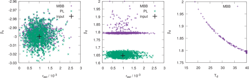
Figure 1: Values of $r$ and the mean foreground parameters obtained from 1000 random realizations of the CMB. No instrumental noise is included. The simulation also includes power-law synchrotron and power-law dust with spatially-varying indices, and the mean indices are $\bar{\beta}_{\rm s}=-3.0$ and $\bar{\beta}_{\rm d}=1.647$. While we always use the Delta-map method for a power-law spectrum (Sect. 2.2) for synchrotron, we compare two Delta-map methods for dust: power-law and MBB (Sect. 2.4). The input map for dust is always a power-law (only in this test). The green (denoted as “PL”) and purple (denoted as “MBB”) points show the results from the Delta-map method for power-law dust and MBB dust, respectively. We use flat priors with $r=[0,1]$, $\bar{\beta}_{\rm s}=[-4,-2]$, $\bar{\beta}_{\rm d}=[1,2]$, and $T_{\rm d}=[10~{}{\rm K},40~{}{\rm K}]$.

Next, we apply the Delta-map method for a MBB for dust (Sect. 2.4), while the simulated maps always have a power-law dust (only in this section). For this case we generate another map generated at 400 GHz so that we have the highest three frequencies for dust. We find that we recover the input values of $r$ and $\bar{\beta}_{\rm s}$. This is because, in the limited frequency range considered here, a MBB can mimic a power law with a spectral index of $1.647$ by appropriately tuning $\bar{\beta}_{\rm d}$ and $\bar{T}_{\rm d}$. (MBB becomes a power law in the Rayleigh-Jeans limit, i.e., $k_{B}T_{\rm d}/h\nu\to\infty$.) The clear correlation seen in the right panel of Fig. 1 supports this interpretation.

4 Bayesian derivation of the Delta-map method

4.1 Likelihood

So far we have formulated the Delta-map method in a “bottom-up approach”; namely, we started with a plausible form of a foreground-cleaned CMB map given in Eq. (11) and constructed a likelihood given in Eq. (28). In this section we formulate the Delta-map method in a “top-down approach” by starting with the likelihood of data $\vec{m}$ given general sky signal $\vec{s}$, mixing matrix $\bm{D}$, and noise covariance matrix $\bm{N}$:

$$-2\ln{\cal L}(\vec{m}|\vec{s},\bm{D})=\left(\vec{m}-\bm{D}\vec{s}\right)^{\rm T}\bm{N}^{-1}\left(\vec{m}-\bm{D}\vec{s}\right)+\ln|2\pi\bm{N}|\,.$$ (40)

We have concatenated the Stokes parameter data at all pixels and frequencies as

$$\vec{m}\equiv\left(\{[Q,U]_{\nu_{1}}(\hat{n}_{i})]\},\cdots,\{[Q,U]_{\nu_{N_{\rm freq}}}(\hat{n}_{i})\}\right)^{\rm T}\,.$$ (41)

We similarly concatenate the noise covariance matrix $\bm{N}$, which now becomes a $2N_{\rm pix}N_{\rm freq}$-by-$2N_{\rm pix}N_{\rm freq}$ matrix. (The factor of 2 is for $Q$ and $U$.) Here, $N_{\rm pix}$ is the number of pixels and $N_{\rm freq}$ is the number of frequency channels, and $\hat{n}_{i}$ is a sky direction unit vector toward $i$th pixel. We have also defined the sky signal vector as

$$\vec{s}\equiv\left(\{\mbox{CMB}(\hat{n}_{i})\},\{\mbox{Dust}(\hat{n}_{i})\},\{\mbox{Synch}(\hat{n}_{i})\},\cdots\right)^{\rm T}\,,$$ (42)

whose number of elements is $2N_{\rm pix}(N_{\rm temp}+1)$, where $N_{\rm temp}$ is the number of foreground (“template”) components. When we have synchrotron and dust, $N_{\rm temp}=2$.

The number of rows of the mixing matrix $\bm{D}$ is $2N_{\rm pix}N_{\rm freq}$, and the number of columns is $2N_{\rm pix}(N_{\rm temp}+1)$. We may write $\bm{D}$ using $2N_{\rm pix}N_{\rm freq}$-by-$2N_{\rm pix}$ sub-matrices as

$${\bm{D}}=\begin{pmatrix}\bm{D}^{\rm CMB}&\bm{D}^{\rm dust}&\bm{D}^{\rm synch}&\cdots\end{pmatrix}\,,$$ (43)

where

$${\bm{D}}^{\rm CMB}\equiv\begin{pmatrix}1&0&\cdots&0\\ 0&1&\cdots&0\\ \vdots&\vdots&\ddots&\vdots\\ 0&0&\cdots&1\\ 1&0&\cdots&0\\ 0&1&\cdots&0\\ \vdots&\vdots&\ddots&\vdots\\ 0&0&\cdots&1\\ \vdots&\vdots&\vdots&\vdots\end{pmatrix}\,,$$ (44)

$${\bm{D}}^{\rm dust}\equiv\begin{pmatrix}g_{\nu_{1}}D^{\rm dust}_{\nu_{1}}(\beta_{{\rm d},1},T_{{\rm d},1},\cdots)&0&\cdots&0\\ 0&g_{\nu_{1}}D^{\rm dust}_{\nu_{1}}(\beta_{{\rm d},2},T_{{\rm d},2},\cdots)&\cdots&0\\ \vdots&\vdots&\ddots&\vdots\\ 0&0&\cdots&g_{\nu_{1}}D^{\rm dust}_{\nu_{1}}(\beta_{{\rm d},N_{\rm pix}},T_{{\rm d},N_{\rm pix}},\cdots)\\ g_{\nu_{2}}D^{\rm dust}_{\nu_{2}}(\beta_{{\rm d},1},T_{{\rm d},1},\cdots)&0&\cdots&0\\ 0&g_{\nu_{2}}D^{\rm dust}_{\nu_{2}}(\beta_{{\rm d},2},T_{{\rm d},2},\cdots)&\cdots&0\\ \vdots&\vdots&\ddots&\vdots\\ 0&0&\cdots&g_{\nu_{2}}D^{\rm dust}_{\nu_{2}}(\beta_{{\rm d},N_{\rm pix}},T_{{\rm d},N_{\rm pix}},\cdots)\\ \vdots&\vdots&\vdots&\vdots\end{pmatrix}\,,$$ (45)

and similarly for $\bm{D}^{\rm synch}$. Here, $\beta_{{\rm d},i}\equiv\beta_{{\rm d}}(\hat{n}_{i})$ etc., and each block in $\bm{D}^{\rm dust}$ should include the entries for both $Q$ and $U$, i.e., each block is a $2N_{\rm pix}$-by-$2N_{\rm pix}$ matrix.

The effect we have not written explicitly here is the effect of a gain calibration, beam smearing, pixel window function, or any extra smoothing/filtering applied to data. These effects will modify all elements of the mixing matrix; e.g., “$1$” in the CMB matrix becomes a product of the calibration factor, beam transfer and pixel window function operators, etc.

The next step is to expand the mixing matrix to first order in spatial variations of the spectral parameters. We redefine the signal vectors as

$$\vec{s}\to\Big{(}\{\mbox{CMB}(\hat{n}_{i})\}, \{\mbox{Dust}(\hat{n}_{i})\},\{\mbox{Dust}(\hat{n}_{i})\delta\beta_{{\rm d},i}\},\{\mbox{Dust}(\hat{n}_{i})\delta T_{{\rm d},i}\},\cdots,$$

$$\{\mbox{Synch}(\hat{n}_{i})\},\{\mbox{Synch}(\hat{n}_{i})\delta\beta_{{\rm s},i}\},\{\mbox{Synch}(\hat{n}_{i})\delta C_{{\rm s},i}\},\cdots\Big{)}^{\rm T}\,,$$ (46)

as well as the mixing matrix as

$${\bm{D}}\to\begin{pmatrix}\bm{D}^{\rm CMB}&\bm{D}^{\rm dust}(\bar{p}^{I})&\bm{D}^{\rm dust}_{,1}&\cdots&\bm{D}^{\rm dust}_{,N}&\bm{D}^{\rm synch}(\bar{p}^{J})&\bm{D}^{\rm synch}_{,1}&\cdots&\bm{D}^{\rm synch}_{,M}&\cdots\end{pmatrix}\,,$$ (47)

where dust and synchrotron have $N$ ($I=1,\cdots,N$) and $M$ ($J=1,\cdots,M$) spectral parameters, respectively. The subscript “$,I$” denotes derivatives with respect to the $I$th foreground parameter (e.g., $\beta_{\rm d}$ and $T_{\rm d}$ for dust and $\beta_{\rm s}$ and $C_{\rm s}$ for synchrotron). All elements in this new mixing matrix are evaluated at the mean spectral parameters. The form of the likelihood given in Eq. (40) remains unchanged.

Specifically,

$$\begin{pmatrix}\bm{D}^{\rm dust}(\bar{p}^{I})&\bm{D}^{\rm dust}_{,1}&\cdots&\bm{D}^{\rm dust}_{,N}\end{pmatrix}$$

$$= \begin{pmatrix}g_{\nu_{1}}D^{\rm dust}_{\nu_{1}}(\bar{p}^{I})\bm{I}&g_{\nu_{1}}D^{\rm dust}_{\nu_{1},1}\bm{I}&\cdots&g_{\nu_{1}}D^{\rm dust}_{\nu_{1},N}\bm{I}\\ g_{\nu_{2}}D^{\rm dust}_{\nu_{2}}(\bar{p}^{I})\bm{I}&g_{\nu_{2}}D^{\rm dust}_{\nu_{2},1}\bm{I}&\cdots&g_{\nu_{2}}D^{\rm dust}_{\nu_{2},N}\bm{I}\\ \vdots&\vdots&\ddots&\vdots\\ g_{\nu_{\rm Nfreq}}D^{\rm dust}_{\nu_{N_{\rm freq}}}(\bar{p}^{I})\bm{I}&g_{\nu_{N_{\rm freq}}}D^{\rm dust}_{\nu_{N_{\rm freq}},1}\bm{I}&\cdots&g_{\nu_{N_{\rm freq}}}D^{\rm dust}_{\nu_{N_{\rm freq}},N}\bm{I}\end{pmatrix}\,,$$ (48)

and similarly for synchrotron etc. Here, $\bm{I}$ is a $2N_{\rm pix}$-by-$2N_{\rm pix}$ identity matrix.

When we have only CMB, dust and synchrotron in the sky, the number of elements of $\vec{s}$ is $2N_{\rm pix}(N+M+3)$ and $\bm{D}$ becomes a $2N_{\rm pix}N_{\rm freq}$-by-$2N_{\rm pix}(N+M+3)$ matrix. When $N_{\rm freq}=N+M+3$, $\bm{D}$ becomes a square matrix and invertible. This is a special case in which the number of frequency channels is just enough to solve for a cleaned CMB map.

Now that the mixing matrix $\bm{D}$ does not depend on pixels, Eq. (40) can be written trivially in pixel, spherical harmonics, or wavelet space. This is an important advantage of linearization used by the Delta-map method.

4.2 Delta-map as the maximum likelihood solution

Maximizing the likelihood with respect to the CMB signal, we obtain 2009MNRAS.392..216S

$$\mbox{CMB}^{\rm ML}(\hat{n})=\left[(\bm{D}^{\rm T}\bm{N}^{-1}\bm{D})^{-1}\bm{D}^{\rm T}\bm{N}^{-1}\vec{m}\right]_{\rm CMB}\,,$$ (49)

where the subscript “CMB” indicates that we take the elements relevant to the CMB, and the superscript “ML” stands for the maximum likelihood value. We can evaluate this in pixel, spherical harmonics, or wavelet space.

When the number of frequency channels is just enough to solve for a cleaned CMB map, $\bm{D}$ is invertible and we obtain $\mbox{CMB}^{\rm ML}=\left[\bm{D}^{-1}\vec{m}\right]_{\rm CMB}$. For example, when we have a spatially uniform power-law component as foreground, the solution for a cleaned CMB map from two maps at two frequencies is

$$\mbox{CMB}^{\rm ML}(\hat{n})=\frac{g_{\nu_{2}}D_{\nu_{2}}m_{\nu_{1}}(\hat{n})-g_{\nu_{1}}D_{\nu_{1}}m_{\nu_{2}}(\hat{n})}{g_{\nu_{2}}D_{\nu_{2}}-g_{\nu_{1}}D_{\nu_{1}}}\,,$$ (50)

where $D_{\nu}=(\nu/\nu_{*})^{\bar{\beta}}$. Note that $\nu_{*}$ cancels. If we identify $\nu_{2}$ with the reference frequency $\nu_{*}$, the expression further simplifies to $\mbox{CMB}^{\rm ML}(\hat{n})=[m_{\nu_{1}}(\hat{n})-(g_{\nu_{1}}/g_{\nu_{*}})D_{\nu_{1}}m_{\nu_{2}}(\hat{n})]/[1-(g_{\nu_{1}}/g_{\nu_{*}})D_{\nu_{1}}]$, which coincides with the usual internal template cleaning solution with $\alpha=(g_{\nu_{1}}/g_{\nu_{*}})D_{\nu_{1}}$ (see, e.g., Eq. (6) of 2011ApJ…737…78K ). We can obtain the same result from Eq. (11) with $\alpha$ given by $-\bm{A}^{-1}\vec{d}_{\nu_{\rm CMB}}$ and $\nu_{1}=\nu_{\rm CMB}$.

When we have a spatially-varying power-law component as foreground, the solution for a cleaned CMB map from three maps at three frequencies is

$$\mbox{CMB}^{\rm ML}(\hat{n})=\frac{\xi_{12}m_{\nu_{3}}(\hat{n})+\xi_{31}m_{\nu_{2}}(\hat{n})-\xi_{23}m_{\nu_{1}}(\hat{n})}{\xi_{12}+\xi_{31}-\xi_{23}}\,,$$ (51)

where $\xi_{ij}\equiv g_{\nu_{i}}g_{\nu_{j}}\left(D_{\nu_{i},\beta}D_{\nu_{j}}-D_{\nu_{i}}D_{\nu_{j},\beta}\right)=g_{\nu_{i}}g_{\nu_{j}}\left(\nu_{i}\nu_{j}/\nu_{*}^{2}\right)^{\bar{\beta}}\ln(\nu_{i}/\nu_{j})$. The numerator evaluates to

$$g_{\nu_{1}}g_{\nu_{2}}(\nu_{1}\nu_{2})^{\bar{\beta}}\ln\left(\frac{\nu_{1}}{\nu_{2}}\right)m_{\nu_{3}}(\hat{n})$$

$$+ g_{\nu_{3}}g_{\nu_{1}}(\nu_{3}\nu_{1})^{\bar{\beta}}\ln\left(\frac{\nu_{3}}{\nu_{1}}\right)m_{\nu_{2}}(\hat{n})-g_{\nu_{2}}g_{\nu_{3}}(\nu_{2}\nu_{3})^{\bar{\beta}}\ln\left(\frac{\nu_{2}}{\nu_{3}}\right)m_{\nu_{1}}(\hat{n})\,,$$ (52)

where we have canceled $\nu^{*}$ with that in the denominator. We find that this result reproduces the numerator of Eq. (17), $[Q,U]_{\nu_{\rm CMB}}+\sum_{j=1}^{2}[Q,U]_{\nu_{j}}$, up to a multiplicative factor if we identify $\nu_{3}$ with $\nu_{\rm CMB}$.

We thus conclude that Eq. (11) gives the maximum likelihood solution for a cleaned CMB map to first order in perturbation, provided that the number of frequency channels is just enough to solve for a cleaned CMB map. We need to use Eq. (49) when we have more channels, which would give a less noisy CMB map.

4.3 Should we cancel CMB in a template map?

SEVEM (see Appendix A.6 of 2008A&A…491..597L ) is an internal template method used by the Planck collaboration. In this method one constructs a template foreground map by first taking difference between two frequency channels (so that CMB cancels) and fits this difference map to a CMB channel and subtracts the foreground. Specifically, when we have one foreground component and three frequency channels, SEVEM constructs

$$\mbox{CMB}^{\rm SEVEM}(\hat{n})=m_{\nu_{1}}(\hat{n})-\alpha\left[m_{\nu_{2}}(\hat{n})-m_{\nu_{3}}(\hat{n})\right]\,,$$ (53)

where $\alpha$ is a fitting coefficient. (For this case, $\nu_{\rm CMB}=\nu_{1}$.) When the foreground has a spatially uniform spectrum, the coefficient is $\alpha=g_{\nu_{1}}D_{\nu_{1}}/(g_{\nu_{2}}D_{\nu_{2}}-g_{\nu_{3}}D_{\nu_{3}})$, which gives an unbiased estimate of CMB.

We find that this is not the maximum likelihood solution given in Eq. (49). Assuming that the noise covariance matrix is diagonal and homogeneous over pixels, $\bm{N}={\rm diag}(\sigma_{\nu_{1}}^{2}\bm{I},\sigma_{\nu_{2}}^{2}\bm{I},\sigma_{\nu_{3}}^{2}\bm{I})$, where $\bm{I}$ is a $2N_{\rm pix}$-by-$2N_{\rm pix}$ identity matrix, Eq. (49) becomes

$$\mbox{CMB}^{\rm ML}(\hat{n})=\frac{(g_{\nu_{1}}D_{\nu_{1}}-g_{\nu_{2}}D_{\nu_{2}})\left[g_{\nu_{1}}D_{\nu_{1}}m_{\nu_{2}}(\hat{n})-g_{\nu_{2}}D_{\nu_{2}}m_{\nu_{1}}(\hat{n})\right]\sigma_{\nu_{3}}^{2}+(\mbox{2 perm.})}{(g_{\nu_{1}}D_{\nu_{1}}-g_{\nu_{2}}D_{\nu_{2}})^{2}\sigma_{\nu_{3}}^{2}+(\mbox{2 perm.})}\,,$$ (54)

where “2 perm.” indicates two permutation terms. While this may look complicated, there is a clear interpretation. To see this, let us define

$$\mbox{CMB}^{\rm ML,2band}_{ij}(\hat{n})\equiv\frac{g_{\nu_{i}}D_{\nu_{i}}m_{\nu_{j}}(\hat{n})-g_{\nu_{j}}D_{\nu_{j}}m_{\nu_{i}}(\hat{n})}{g_{\nu_{i}}D_{\nu_{i}}-g_{\nu_{j}}D_{\nu_{j}}}\,,$$ (55)

which is the Maximum likelihood solution when we have only two frequency channels $\nu_{i}$ and $\nu_{j}$ (Eq. (50)). We find

$$\mbox{CMB}^{\rm ML}(\hat{n})=\frac{(g_{\nu_{1}}D_{\nu_{1}}-g_{\nu_{2}}D_{\nu_{2}})^{2}\mbox{CMB}^{\rm ML,2band}_{12}(\hat{n})\sigma_{\nu_{3}}^{2}+(\mbox{2 perm.})}{(g_{\nu_{1}}D_{\nu_{1}}-g_{\nu_{2}}D_{\nu_{2}})^{2}\sigma_{\nu_{3}}^{2}+(\mbox{2 perm.})}\,.$$ (56)

Therefore, the maximum likelihood solution is equal to three cleaned CMB maps combined optimally, but is not equal to the SEVEM construction.

4.4 Posterior of the parameters

The next task is to derive a posterior distribution of the mean spectral parameters $\bar{p}^{I}$ and the cosmological parameters such as the tensor-to-scalar ratio $r$. We start by using Bayes’s theorem to relate the posterior distribution to the likelihood given in Eq. (40) as

$$P(\bar{p}^{I},\vec{s},\bm{S}|\vec{m})=\frac{{\cal L}(\vec{m}|\vec{s},\bm{D})P(\bm{D},\vec{s},\bm{S})}{P(\vec{m})}\,,$$ (57)

where $\bm{S}$ is a covariance matrix of the sky signal $\vec{s}=\vec{s}_{\rm CMB}+\vec{s}_{f}$ (CMB $\vec{s}_{\rm CMB}$ and foregrounds $\vec{s}_{f}$), $P(\bm{D},\vec{s},\bm{S})$ is the prior distribution, and $P(\vec{m})$ is Bayes’s (normalization) factor. Note that $\bar{p}^{I}$ is a vector of the parameters that determine the mixing matrix $\bm{D}$. We shall assume a flat prior on $\bm{D}$, i.e., $P(\bm{D},\vec{s},\bm{S})\propto P(\vec{s},\bm{S})$.

We first marginalize Eq. (57) over the CMB signal. To this end we assume a Gaussian probability density distribution for the CMB signal part of the prior: $-2\ln P(\vec{s},\bm{S})=\vec{s}_{\rm CMB}(\bm{S}_{0}^{\rm CMB})^{-1}\vec{s}_{\rm CMB}+\ln|2\pi\bm{S}_{0}^{\rm CMB}|+(\mbox{other terms})$, where $\bm{S}_{0}^{\rm CMB}$ is a $2N_{\rm pix}$-by-$2N_{\rm pix}$ CMB signal covariance matrix with no beam smearing, pixel window function, extra filtering, or calibration factor.

Integrating both sides of Eq. (57) over $\vec{s}_{\rm CMB}$, we obtain

$$-2\ln P(\bar{p}^{I},\vec{s}_{f},\bm{S}|\vec{m}) = \left(\vec{m}-\tilde{\bm{D}}\vec{s}_{f}\right)^{\rm T}\left(\bm{S}^{\rm CMB}+\bm{N}\right)^{-1}\left(\vec{m}-\tilde{\bm{D}}\vec{s}_{f}\right)$$ (58)

$$+\ln\left|2\pi(\bm{S}^{\rm CMB}+\bm{N})\right|-2\ln P(\vec{s}_{f},\bm{S}^{f})+\mbox{constant}\,,$$

where $\bm{S}^{\rm CMB}=\bm{D}^{\rm CMB}\bm{S}^{\rm CMB}_{0}(\bm{D}^{\rm CMB})^{\rm T}$, $\vec{s}_{f}$ is the foreground sky signal vector with $P(\vec{s}_{f},\bm{S}^{f})$ being its prior, and $\tilde{\bm{D}}$ is a new mixing matrix eliminating CMB, i.e.,

$$\tilde{\bm{D}}\equiv\begin{pmatrix}\bm{D}^{\rm dust}(\bar{p}^{I})&\bm{D}^{\rm dust}_{,1}&\cdots&\bm{D}^{\rm dust}_{,N}&\bm{D}^{\rm synch}(\bar{p}^{J})&\bm{D}^{\rm synch}_{,1}&\cdots&\bm{D}^{\rm synch}_{,M}&\cdots\end{pmatrix}\,.$$ (59)

Note that $\tilde{\bm{D}}$ is not a square matrix and thus not invertible. For example, when we have only dust and synchrotron as foregrounds, and dust and synchrotron have $N$ and $M$ spectral parameters, respectively, $\tilde{\bm{D}}$ becomes a $2N_{\rm pix}N_{\rm freq}$-by-$2N_{\rm pix}(N+M+2)$ matrix; however, to be able to solve for a cleaned CMB map we need $N_{\rm freq}\geq N+M+3$.

We maximize the marginalized likelihood part of Eq. (58) (the first line on the right hand side) with respect to the foreground sky signal to obtain the maximum likelihood value of $\vec{s}_{f}$ as

$$\vec{s}_{f}^{\rm ML}=\left[\tilde{\bm{D}}^{\rm T}(\bm{S}^{\rm CMB}+\bm{N})^{-1}\tilde{\bm{D}}\right]^{-1}\tilde{\bm{D}}^{\rm T}(\bm{S}^{\rm CMB}+\bm{N})^{-1}\vec{m}\,.$$ (60)

Note that $\vec{s}_{f}^{\rm ML}$ is not the maximum likelihood value of Eq. (40) but is the maximum likelihood value of the CMB-marginalized likelihood, Eq. (58), ignoring the prior term.

Inserting $\vec{s}_{f}^{\rm ML}$ back into Eq. (58), we obtain the final expression for the posterior distribution:

$$-2\ln P(\bar{p}^{I},\vec{s}^{\rm ML}_{f},\bm{S} |\vec{m})=\vec{m}^{\rm T}\left(\bm{S}^{\rm CMB}+\bm{N}\right)^{-1}\vec{m}$$

$$-\left[\tilde{\bm{D}}^{\rm T}(\bm{S}^{\rm CMB}+\bm{N})^{-1}\vec{m}\right]^{\rm T}\left[\tilde{\bm{D}}^{\rm T}(\bm{S}^{\rm CMB}+\bm{N})^{-1}\tilde{\bm{D}}\right]^{-1}\tilde{\bm{D}}^{\rm T}(\bm{S}^{\rm CMB}+\bm{N})^{-1}\vec{m}$$

$$+\ln\left|2\pi(\bm{S}^{\rm CMB}+\bm{N})\right|-2\ln P(\vec{s}_{f}^{\rm ML},\bm{S}^{f})+\mbox{constant}\,.$$ (61)

This formula is the foundation of the Delta-map method. Once again, as $\tilde{\bm{D}}$ no longer depends on sky directions $\hat{n}$, we can evaluate the posterior in pixel, spherical harmonics, or wavelet space by using $\vec{m}$, $\bm{S}^{\rm CMB}$, and $\bm{N}$ in the appropriate basis.

To understand this rather complicated expression, let us use an example of a spatially uniform power-law component as foreground and work with two maps at two frequencies. Then the first two lines yield

$$\mbox{CMB}^{\rm ML}\left[\bm{S}_{0}^{\rm CMB}+\frac{g_{\nu_{2}}^{2}D^{2}_{\nu_{2}}{\bm{N}}_{\nu_{1}}+g_{\nu_{1}}^{2}D^{2}_{\nu_{1}}{\bm{N}}_{\nu_{2}}}{\left(g_{\nu_{2}}D_{\nu_{2}}-g_{\nu_{1}}D_{\nu_{1}}\right)^{2}}\right]^{-1}\mbox{CMB}^{\rm ML}\,,$$ (62)

where $\mbox{CMB}^{\rm ML}$ is given by Eq. (50). We find that this expression agrees with the likelihood we constructed in Eq. (28) with appropriate coefficients $\alpha_{j}$ for this example, up to the diagonal noise (which we have not added here yet). Therefore, we conclude that Eq. (28) gives the CMB-marginalized posterior distribution of $\bar{p}^{I}$ and the cosmological parameters, with the maximum likelihood estimate of foregrounds for the CMB-marginalized likelihood.

As the determinant term in Eq. (61) does not depend on the mixing matrix (hence $\bar{p}^{I}$), maximizing the posterior with respect to $\bar{p}^{I}$ with a flat prior, $P(\vec{s}_{f},\bm{S}^{f})=\mbox{constant}$, amounts to minimizing $\chi^{2}$ as in Eq. (33). This justifies our algorithm presented in Sect. 3.

We could have marginalized Eq. (58) over $\vec{s}_{f}$. Then it would also modify the determinant which, in turn, would depend on $\bar{p}^{I}$. This would be the situation in which we maximize Eq. (28) including the determinant for $\bar{p}^{I}$, $r$, and $s$ simultaneously. However, we find that this procedure produces a biased result for $\bar{p}^{I}$. The same behavior was observed in 2009MNRAS.392..216S for a flat prior on $\vec{s}_{f}$. An intuitive reason for this is that, when foregrounds are allowed to vary to unreasonably large values by a flat prior, the marginalized distribution has $\bar{p}^{I}$ that is far away from the maximum likelihood values. Therefore, a better approach would be either to use $\vec{s}^{\rm ML}_{f}$ instead of marginalizing over it (which we have adopted here), or to marginalize over $\vec{s}_{f}$ with a reasonable choice of $\bm{S}^{f}$ (see 2016A&A…588A.113V ; vansyngelthesis:2014 for this approach), or to marginalize over $\bm{S}^{f}$.

Note that the posterior distribution given in Eq. (61) does not make distinction between “CMB channels”, “synchrotron channels”, and “dust channels”. This is a nice feature; while a heuristic construction of cleaned CMB maps based on identifying low- and high-frequency maps as foreground channels (discussed in Sect. 2) as well as its likelihood given in Eq. (28) is intuitive and easy to understand/interpret, it might give readers an impression that there is some arbitrariness in choosing which channels are CMB etc. Consider the case where we have far more channels than the number of foreground components. Then, how should we decide which ones are CMB and foreground channels? The posterior distribution we have derived in this section tells us that this arbitrariness does not exist: we can use Eq. (61) to combine all the data optimally to estimate $r$ and the mean foreground parameters.

For the rest of this paper, we shall explore the simplest cases in which the number of frequency channels is just enough to solve for one CMB map and the necessary number of the mean foreground parameters. Then Eq. (28) is the appropriate likelihood. That is to say, $N_{\rm freq}=N+M+3$. For more general cases in which $N_{\rm freq}$ is greater, Eq. (61) should be used.

5 Validation with realistic foreground maps

5.1 Sky model

Our fiducial sky model consists of three components: polarized CMB, synchrotron, and thermal dust emission. Later in Sect. 6.2, we also explore the effect of AME on cleaning synchrotron.

For synchrotron, we use “SynchrtronPol-commander_0256_R2.00” at $30$ GHz as a template, which was derived from Planck maps using the Commander algorithm 2016A&A…594A..10P . We extrapolate this map to other frequencies assuming power-law emission with spatially-varying spectral indices $\beta_{\rm s}$. The spatial variation is taken from 2008A&A…490.1093M , which was derived from WMAP 23 GHz and Haslam 408 MHz maps.

For dust component, we explore two possibilities: one-component and two-component MBB dust. The latter is to test robustness of the Delta-map method for more complex sky model; namely, we build the Delta-map method assuming one component, and apply it to a sky map containing two-component dust. Our starting point is the dust polarization template “DustPol-commander_1024_R2.00” at $353$ GHz, which was derived from Planck maps using the Commander algorithm 2016A&A…594A..10P . Extrapolation to other frequencies is done by either one- or two-component MBB.

The one-component MBB is given by Eq. (21), with maps of $\beta_{\rm d}(\hat{n})$ and $T_{\rm d}(\hat{n})$ taken from the Commander analysis given in 2016A&A…594A..10P .

A two-component MBB model is motivated by an observation that the one-component model does not explain simultaneously the Rayleigh-Jeans (microwave) and Wien (infrared) regions of the dust spectrum observed by the FIRAS and DIRBE instruments on board COBE, respectively 1999ApJ…524..867F . A two-component MBB dust model has been proposed to explain the observations. Physically, two components might represent different dust grains (e.g., silicate- and carbon-dominated grains) with different temperatures. Our two-component model is based on 2015ApJ…798…88M . The model assumes the following frequency dependence in brightness temperature:

$$F_{\nu}=a_{1}\left(\frac{\nu}{\nu_{0}}\right)^{\beta_{1}+1}\frac{1}{e^{h\nu/k_{B}T_{1}(\hat{n})}-1}+a_{2}\left(\frac{\nu}{\nu_{0}}\right)^{\beta_{2}+1}\frac{1}{e^{h\nu/k_{B}T_{2}(\hat{n})}-1}~{},$$ (63)

with $\nu_{0}=c/\lambda_{0}$ and $\lambda_{0}=100~{}\mu{\rm m}$. This function then gives $D_{\nu}=F_{\nu}/F_{\nu_{*}}$. Here, $a_{1}$, $a_{2}$, $\beta_{1}$, and $\beta_{2}$ are constant fitting parameters, whereas $T_{2}(\hat{n})$ (hot dust temperature) is a spatially-varying parameter. The remaining parameter, $T_{1}(\hat{n})$ (cold dust temperature), is derived from $T_{2}$ assuming thermal equilibrium with the same interstellar-radiation field 1999ApJ…524..867F , i.e.,

$$[T_{1}(\hat{n})]^{4+\beta_{1}}=\frac{1}{q_{r}}\frac{\zeta(4+\beta_{2})}{\zeta(4+\beta_{1})}\frac{\Gamma(4+\beta_{2})}{\Gamma(4+\beta_{1})}\left(\frac{h\nu_{0}}{k_{B}}\right)^{\beta_{1}-\beta_{2}}[T_{2}(\hat{n})]^{4+\beta_{2}}~{}.$$ (64)

Here we have set the constant parameters as $\beta_{2}=2.82$, $\beta_{1}=1.63$, $a_{1}=f_{1}q_{r}$, $a_{2}=(1-f_{1})$ with $f_{1}=0.0485$, and $q_{r}=8.219$ 2015ApJ…798…88M . The spatially varying parameters $T_{2}(\hat{n})$ and $[Q^{f},U^{f}]_{\nu_{*}}(\hat{n})$ with $\nu_{*}=353$ GHz are set according to the Planck results 2015ApJ…798…88M .

5.2 Results

We apply the Delta-map method to estimate $r$ from 1000 random realizations of the CMB at a Healpix resolution of $N_{\rm side}=4$. We do not include instrumental noise here but investigate the effect of noise in Sect. 7. We prepare two sets of simulations: one with no tensor mode ($r_{\rm input}=0$) and another with $r_{\rm input}=10^{-3}$.

We smooth foreground maps and resample them at low-resolution pixels of $N_{\rm side}=4$ following the procedure described in Sect. 3. We use the P06 mask defined by the WMAP polarization analysis 2007ApJS..170..335P and implement it in the likelihood evaluation following Appendix A.

We compare two combinations of frequencies: $(40,60,140,230,280,340)$ GHz (Case A) and $(40,60,140,230,340,400)$ GHz (Case B). We show the results for $\nu_{\rm CMB}=140$ GHz in this paper but one can choose other $\nu_{\rm CMB}$. We do not apply bandpass average. In this and following sections, we explore the likelihood in the parameter ranges of $r=[0,1]$, $\beta_{\rm s}=[-4.0,-2.0]$, $\beta_{\rm d}=[1.0,2.0]$ and $T_{\rm d}=[5~{}{\rm K},40~{}{\rm K}]$ to find the best-fitting parameters for each realization. We find that all the best-fitting parameters are well within these parameter ranges listed above for all the 1000 realizations.

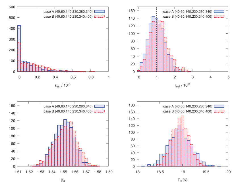
Figure 2: Performance of the Delta-map method for power-law synchrotron and one-component MBB dust. (Upper panels) We show the distribution of $r$ estimated from 1000 random realizations of the CMB. No instrumental noise is included. The simulation also includes power-law synchrotron and one-component MBB dust. (Left) The input value of $r$ is zero. (Right) The input value of $r$ is $10^{-3}$. We show the results for $\nu_{\rm CMB}=140$ GHz. The other channels are indicated in the figure. (Bottom panels) The distribution of $\bar{\beta}_{\rm d}$ and $\bar{T}_{\rm d}$ estimated from 1000 random realizations, for the input value of $r=0$.

In Fig. 2, we show the results from applying the Delta-map method for power-law synchrotron (Sect. 2.2) and one-component MBB (Sect. 2.4) to CMB$+$power-law synchrotron$+$one-component MBB simulations, i.e., the simulations and assumptions match up to first order in spatial variation of the foreground parameters. For $r_{\rm input}=0$ (left panel), we find no significant bias, with a slightly larger uncertainty in $r$ for Case B. The uncertainties are dominated by cosmic variance of the gravitational lensing effect 2011ApJ…737…78K and are found to be $r<0.34\times 10^{-3}$ for Case A and $r<0.48\times 10^{-3}$ for Case B (95% CL). These results are much better than our previous study that found a significant bias for the P06 mask, $\delta r=2\times 10^{-3}$ 2011ApJ…737…78K , because our previous algorithm had to assume that the spectral parameters are uniform across the sky. The Delta-map method takes care of the spatial variation of the spectral parameters, as promised. Note that, for $r_{\rm input}=0$, a large number of samples fall into the first bin because foregrounds are successfully removed and we have put a hard prior of $r\geq 0$.

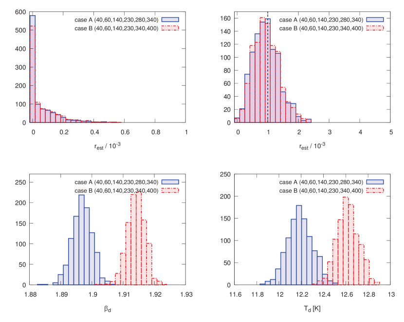
Figure 3: Same as Fig. 2, but the Delta-map method is applied to simulations with CMB$+$power-law synchrotron$+$two-component MBB dust. Note that the Delta-map method still assumes that dust is one-component MBB. We show the results for $\nu_{\rm CMB}=140$ GHz. The other channels are indicated in the figure.

For $r_{\rm input}=10^{-3}$ (right panel), we find $r=(1.12\pm 0.45)\times 10^{-3}$ for Case A and $(1.22\pm 0.48)\times 10^{-3}$ for Case B (68% CL). The error bar here is dominated by both CMB lensing and cosmic variance of the input tensor mode.

Next, we apply the Delta-map method for power-law synchrotron and one-component MBB to CMB$+$power-law synchrotron$+$two-component MBB simulations, i.e., the simulations and assumptions no longer match for dust. Can we still recover the input $r$ without a significant bias? In Fig. 3 we show the recovered $r$. For $r_{\rm input}=0$ (left panel) we find $r<0.26\times 10^{-3}$ for Case A and $r<0.31\times 10^{-3}$ for Case B (95% CL). For $r_{\rm input}=10^{-3}$ (right panel) we find $r=(1.02\pm 0.42)\times 10^{-3}$ for Case A and $(1.05\pm 0.43)\times 10^{-3}$ for Case B (68% CL). Interestingly we obtain slightly a better result for this case, but the difference with respect to the previous case is well within the error bar.

We thus conclude that the Delta-map method recovers the input value of $r$ without a significant bias in the presence of realistic spatially-varying foreground spectral parameters. The slight difference in the uncertainties for Case A and B arises from foreground residuals. Generally, in the absence of instrumental noise we expect smaller uncertainties if the foreground channels are closer to the CMB channel, because a mismatch of foreground emission between the CMB and foreground channels decreases as the CMB and foreground channels become closer to one another.

5.3 Null test

To test our algorithm more precisely, we perform a null test; namely, we clean two maps (100 and 140 GHz) following the procedure in Sect. 3.2, estimate $r$, and take the difference to see if there is any residual bias in the difference. This is a powerful null test (see 2009ApJS..180..225H for application to the optical depth parameter $\tau$), as it is free from cosmic variance, allowing for precise test with a smaller error bar. We must perform this kind of test on the real data to make sure that a future detection of $r$ is not due to a residual foreground. As we do not include instrumental noise yet, the estimates of $r$ at $100$ GHz ($r_{100}$) and $140$ GHz ($r_{140}$) should be identical if the foreground emission is removed adequately.

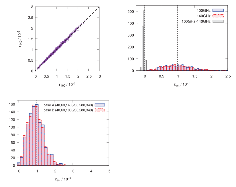
Figure 4: Null test for $r$ measured from cleaned 100 GHz ($r_{100}$) and 140 GHz ($r_{140}$) data. (Upper left) Scatter plot of $r_{100}$ and $r_{140}$. (Upper right) Distribution of $r_{100}$ (purple), $r_{140}$ (green), and $r_{100}-r_{140}$ (red). (Bottom left) A zoom-up of the distributions of $r_{100}$ and $r_{140}$ in the upper right panel, with the same bin size as in the top-right panel of Fig. 3. The input value of $r$ is $10^{-3}$.

We perform the null test for the simulations with $r_{\rm input}=10^{-3}$, power-law synchrotron, and two-component MBB dust (while the Delta-map method assumes one-component MBB). Frequency channels are $(40,60,100,140,230,280,340)$ GHz.

In the left panel of Fig. 4, we show that $r_{100}$ and $r_{140}$ are indeed highly correlated. In the right panel, we show the distribution of the difference, $r_{100}-r_{140}$, as well as those of $r_{100}$ and $r_{140}$. We find that the distribution is consistent with the null hypothesis and that the small spread of the distribution of $r_{100}-r_{140}$ is due to foreground residuals. We find $r_{100}-r_{140}=(0.72\pm 2.98)\times 10^{-5}$ (68% CL).

6 Applications

6.1 Decorrelation

Internal template methods assume that a map of $[Q,U]$ at one frequency can be used to predict $[Q,U]$ at other frequencies as a function of foreground parameters. However, this assumption breaks down and leads to a phenomenon called “decorrelation”, when we have a superposition of multiple components with different foreground parameters; e.g., superposition of multiple dust components with different values of $\beta_{d}$ and $T_{d}$ along the line of sight 2015MNRAS.451L..90T ; 2017PhRvD..95j3511P . The same effect arises when we pixelize (or coarse-grain) a map with big pixels containing many smaller pixels with different values of $\beta_{d}$ and $T_{d}$. Currently there is no evidence for the former, intrinsic decorrelation effect 2018arXiv180104945P , whereas the latter effect can be modeled given the distribution of foreground parameters on smaller pixels. As we shall show in this section, one way to deal with this decorrelation effect is to use the foreground parameters that are slightly different for Stokes $Q$ and $U$.

6.1.1 Theory

Let us take dust as an example, though the results can be generalized straightforwardly to other foreground components. Consider that we have multiple dust components along the line of sight or within a big pixel. Each $i$th component has a temperature $T_{{\rm d},i}$ and a polarization direction $\gamma_{i}$. We then observe

$$Q_{\nu} = \sum_{i}Q_{\nu,i}=g_{\nu}\sum_{i}I_{{\rm d},\nu}(T_{{\rm d},i})\Pi_{i}\cos(2\gamma_{i})\,,$$ (65)

$$U_{\nu} = \sum_{i}U_{\nu,i}=g_{\nu}\sum_{i}I_{{\rm d},\nu}(T_{{\rm d},i})\Pi_{i}\sin(2\gamma_{i})\,,$$ (66)

where $I_{{\rm d}}$ is an unpolarized dust amplitude in brightness temperature units and $\Pi_{i}$ is a polarization fraction. We have omitted the sky direction vector $\hat{n}$ to simplify notation. Here we assume that it is only the dust temperature $T_{{\rm d},i}$ that varies and we fix the dust emissivity $\beta_{{\rm d}}$, but it is straightforward to include it in the final result.

We consider $Q$ first. Writing dust temperatures as $T_{{\rm d},i}=\bar{T}_{{\rm d}}\left(1+\delta_{i}\right)$, we obtain

$$Q_{\nu}=g_{\nu}I_{{\rm d},\nu}(\bar{T}_{\rm d})\sum_{i}\left(1+\frac{x_{\rm d}e^{x_{\rm d}}\delta_{i}}{e^{x_{\rm d}}-1}+\cdots\right)\Pi_{i}\cos(2\gamma_{i})\,,$$ (67)

where $x_{\rm d}\equiv h\nu/(k_{B}\bar{T}_{\rm d})$. Writing $A\equiv\sum_{i}\Pi_{i}\cos(2\gamma_{i})$, we obtain

$$Q_{\nu}=g_{\nu}I_{{\rm d},\nu}(\bar{T}_{\rm d})A\left[1+\frac{x_{\rm d}e^{x_{\rm d}}}{e^{x_{\rm d}}-1}\frac{\sum_{i}\delta_{i}\Pi_{i}\cos(2\gamma_{i})}{\sum_{i}\Pi_{i}\cos(2\gamma_{i})}+\cdots\right]\,.$$ (68)

If we define a new dust temperature fluctuation variable

$${\delta}_{Q}\equiv\frac{\sum_{i}\delta_{i}\Pi_{i}\cos(2\gamma_{i})}{\sum_{i}\Pi_{i}\cos(2\gamma_{i})}\,,$$ (69)

and truncate expansion at first order in $\delta_{i}$, we find $Q_{\nu}=g_{\nu}I_{{\rm d},\nu}({T}_{Q})A$, where ${T}_{Q}\equiv\bar{T}_{\rm d}(1+{\delta}_{Q})$. Performing similar calculations for $U$, we find $U_{\nu}=g_{\nu}I_{{\rm d},\nu}({T}_{U})B$, where $B\equiv\sum_{i}\Pi_{i}\sin(2\gamma_{i})$, ${T}_{U}\equiv\bar{T}_{\rm d}(1+{\delta}_{U})$, and

$${\delta}_{U}\equiv\frac{\sum_{i}\delta_{i}\Pi_{i}\sin(2\gamma_{i})}{\sum_{i}\Pi_{i}\sin(2\gamma_{i})}\,.$$ (70)

Now, we can always write $A$ and $B$ as $A=\Pi\cos(2\gamma)$ and $B=\Pi\sin(2\gamma)$ by defining $\Pi$ and $\gamma$ by $\Pi\equiv\sqrt{A^{2}+B^{2}}$ and $\tan(2\gamma)\equiv B/A$. We obtain the final result:

$$Q_{\nu} = g_{\nu}I_{{\rm d},\nu}({T}_{Q})\Pi\cos(2\gamma)\,,$$ (71)

$$U_{\nu} = g_{\nu}I_{{\rm d},\nu}({T}_{U})\Pi\sin(2\gamma)\,.$$ (72)

Therefore, to first order in temperature perturbation, $Q$ and $U$ behave as if they had slightly different dust temperatures. This makes an observed polarization direction, $\gamma_{\rm obs}$, different from $\gamma$ because

$$2\gamma_{\rm obs}=\tan^{-1}\left[\frac{U(\nu)}{Q(\nu)}\right]=\tan^{-1}\left[\frac{I_{{\rm d},\nu}(T_{U})}{I_{{\rm d},\nu}(T_{Q})}\tan(2\gamma)\right]\,.$$ (73)

Importantly, the observed polarization direction changes with frequency, i.e., $\gamma_{\rm obs}=\gamma_{\rm obs}(\nu)$. This is the origin of frequency decorrelation.

We can account for variations in any other foreground parameters (e.g., $\beta_{\rm d}$, $\beta_{\rm s}$, $C_{\rm s}$) by using slightly different values for $Q$ and $U$.

6.1.2 Impact on $r$

We include decorrelation in our two-component MBB dust simulation as follows. We perturb temperature of hot dust, $T_{2}$, in $Q$ and $U$ as

$$T^{Q}_{2}(\hat{n}) \equiv T_{2}(\hat{n})+\epsilon_{Q}\sigma_{T}~{},$$ (74)

$$T^{U}_{2}(\hat{n}) \equiv T_{2}(\hat{n})+\epsilon_{U}\sigma_{T}~{},$$ (75)

where $\epsilon_{Q}$ and $\epsilon_{U}$ are Gaussian random numbers with unit variance and $\sigma_{T}$ is a parameter that controls the effect of decorrelation. Temperatures of cold dust, $T^{Q}_{1}$ and $T^{U}_{1}$, are related to $T^{Q}_{2}$ and $T^{U}_{2}$ via Eq. (64). Using these temperatures, we extrapolate the Planck dust polarization maps in brightness temperature units at 353 GHz to other frequencies using

$$Q_{\nu}(\hat{n}) = g_{\nu}\frac{I_{{\rm d},\nu}(T^{Q}_{2}(\hat{n}))}{I_{{\rm d},353}(T_{2}(\hat{n}))}Q^{f}_{353}(\hat{n})~{},$$ (76)

$$U_{\nu}(\hat{n}) = g_{\nu}\frac{I_{{\rm d},\nu}(T^{U}_{2}(\hat{n}))}{I_{{\rm d},353}(T_{2}(\hat{n}))}U^{f}_{353}(\hat{n})~{},$$ (77)

where $I_{\nu}(T_{2}(\hat{n}))$ is the frequency spectrum in the two component model given by Eq. (63).

We can implement $T^{Q}_{2}$ and $T^{U}_{2}$ directly into the Delta-map method by increasing the number of mean temperatures from one $\bar{T}_{\rm d}$ to two $\bar{T}^{Q}_{2}$ and $\bar{T}^{U}_{2}$. However, in this section we instead apply the Delta-map method for one temperature $\bar{T}_{\rm d}$ and see how much impact the decorrelation has on our estimation of $r$. To this end, we generate temperature fluctuations with r.m.s. of 1 K, i.e., $\sigma_{T}=1$ K and include them in the hot dust temperature of two-component MBB dust. To avoid negative temperature by fluctuations, we do not perturb it if $T_{2}<5$ K.

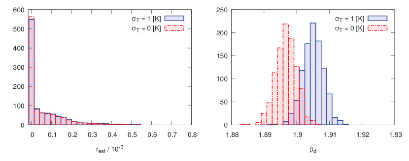
Figure 5: Distribution of $r$ and $\bar{\beta}_{\rm d}$ obtained from 1000 random realizations of the CMB with (purple) and without (green) decorrelation of dust polarization in the simulation. The Delta-map method assumes that there is no decorrelation. We used (40,60,230,280,340) GHz channels to clean $140$ GHz channel. The simulation also includes power-law synchrotron and two-component MBB dust.

In Fig. 5 we find that decorrelation with $\sigma_{T}=1$ K shifts the best-fitting value of $\bar{\beta}_{\rm d}$ (right panel); a superposition of varying foreground parameters changes the average foreground spectrum as shown by 2017MNRAS.472.1195C . Fortunately, this has little impact on $r$ (left panel). This is a good news for estimation of $r$, though the appropriate magnitude of $\sigma_{T}$ in real sky and r.m.s. of other foreground parameters are yet to be determined. At least our method provides a framework within which frequency decorrelation due to any foreground parameters can be treated consistently to first order in perturbation. In table 1, we summarize the mean and variance of the sky-averaged foreground parameters obtained from 1000 random realizations of the CMB with the assumed foreground maps and the frequency channels used in the analysis.

Table 1: Mean and variance of the reconstructed sky-averaged foreground parameters

dust model ($r=0$)	$\bar{\beta}_{s}$	$\bar{\beta}_{d}$	$\bar{T}_{d}$
one-component (case A)	$-2.920\pm 0.020$	$1.5523\pm 0.009$	$18.97\pm 0.24$
one-component (case B)	$-2.906\pm 0.024$	$1.5540\pm 0.010$	$18.99\pm 0.19$
two-component (case A)	$-2.940\pm 0.026$	$1.8977\pm 0.003$	$12.21\pm 0.11$
two-component (case B)	$-2.934\pm 0.029$	$1.9150\pm 0.003$	$12.64\pm 0.10$
two-component (case A with $\sigma_{T}=1$ [K])	$-2.939\pm 0.026$	$1.9059\pm 0.003$	$12.06\pm 0.11$

6.2 AME

While it is widely believed that Galactic synchrotron and thermal dust emissions are the most dominant sources of polarized foreground emission on large angular scales 2014PTEP.2014fB109I , there might be a third polarized component, AME, whose most plausible candidate includes tiny PAH particles spinning with dipole moments 2013AdAst2013E..12L ; 2018NewAR..80….1D . While the AME has been shown to contribute to $\mu$K-level fluctuations in unpolarized intensity at $40$ GHz and even smaller fluctuations at higher frequencies 2013ApJS..208…20B , little is known about its polarization properties.

The Planck collaboration has put an upper bound on the polarization fraction of AME of $\Pi\lesssim 1.6\%$ in the Perseus region 2016A&A…594A..25P . The QUIJOTE collaboration has placed a limit of $\Pi\lesssim 0.39\%$ in the molecular complexes W43 2017MNRAS.464.4107G . The polarization degree in more diffuse areas that are suitable for cosmological analyses is unknown owing to the strong contamination from Galactic synchrotron emission. Even though the polarization contribution of AME to the microwave data near the foreground minimum, $\nu\approx 80-100$ GHz, is expected to be negligible, it affects component separation by changing interpretation of low frequency data from pure synchrotron to synchrotron plus AME. In this sense, AME affects estimation of $r$ indirectly. In this section we show that this indirect effect can be absorbed into the synchrotron curvature parameter $C_{\rm s}$.

To estimate the effect of AME, we model it following 2016MNRAS.458.2032R . Specifically, we take the intensity map of thermal dust emission at $353$ GHz and rescale it by a factor of 0.9 that is found in the Planck 2015 results 2016A&A…594A..25P to predict the AME intensity at 22.8 GHz. We then assign a 1% polarization fraction with the same polarization angles as those of the thermal dust component, with a frequency spectrum given by the cold-medium model described in 2009MNRAS.395.1055A .

We first apply the Delta-map method to the simulation with CMB$+$power-law synchrotron$+$one-component MBB dust$+$AME, using the Delta-map method for power-law synchrotron and one-component MBB dust. We use $(40,60,140,230,280,340)$ GHz. We find a significant bias in the estimated $r$: $r_{\rm est}=0.068\pm 0.011$ (68% CL) for $r_{\rm input}=0$. At first this result was surprising because the amplitude of AME at 140 GHz is too small to be relevant. We then find that AME affects $r$ via changing the best-fitting synchrotron. We therefore added curvature to the synchrotron spectrum and implement it in the Delta-map method following the procedure in Sect. 2.3. Including $C_{\rm s}$ requires one more frequency channel for synchrotron, so we add one more frequency, which is to be determined. When adding $C_{\rm s}$, we need to specify the pivot frequency $\nu_{\rm s}$; we write a curved power-law synchrotron spectrum as $\nu^{\beta_{\rm s}+C_{\rm s}\ln(\nu/\nu_{\rm s})}$. We try $\nu_{\rm s}=40$ and $50$ GHz. Choice of $\nu_{\rm s}$ does not affect the CMB result because it cancels in the cleaned CMB map, but it would change the meaning of synchrotron parameters.

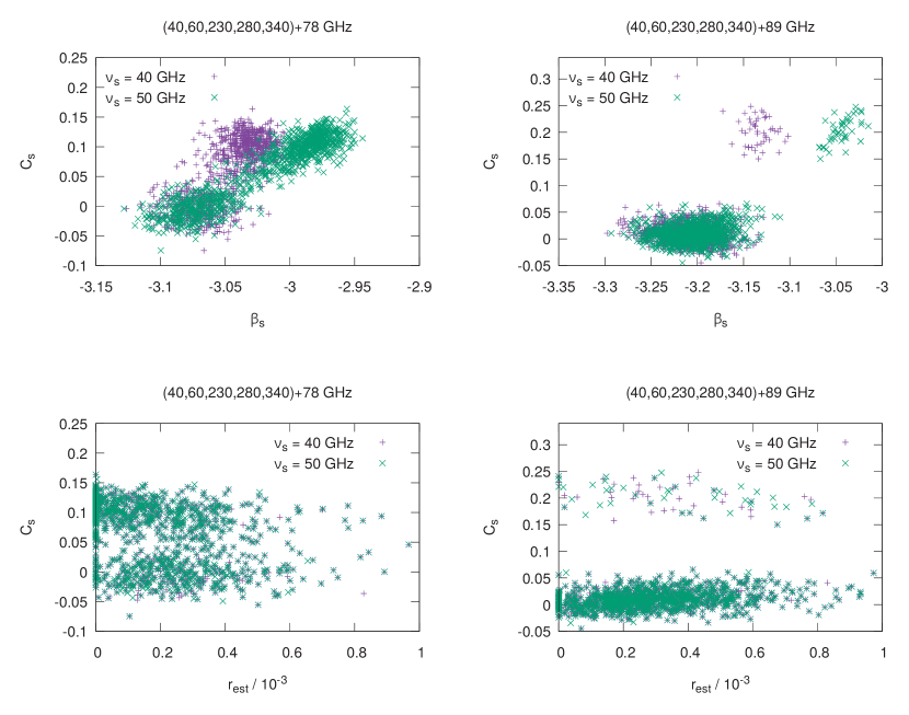
Figure 6: Scatter plots of $\bar{\beta}_{\rm s}$ and $\bar{C}_{\rm s}$ (top panels) and $r$ and $\bar{C}_{\rm s}$ (bottom panels) obtained from 1000 random realizations of the CMB with $r=0$. The simulation also includes AME, power-law synchrotron, and one-component MBB dust. We apply the Delta-map method for curved power-law synchrotron and one-component MBB dust. We show the results for $\nu_{\rm CMB}=140$ GHz. The other frequencies used are shown on top of each panel. We consider two pivot frequencies ($40$ and $50$ GHz), as shown in the figure.

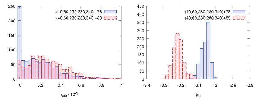
Figure 7: Distribution of $r$ (left) and $\bar{\beta}_{\rm s}$ (right) estimated from 1000 random realizations of the CMB with $r=0$. The simulation also includes AME, power-law synchrotron, and one-component MBB dust. We use the Delta-map method for one-component MBB dust and curved power-law synchrotron with the pivot frequency of $\nu_{\rm s}=40$ GHz. We show the results for $\nu_{\rm CMB}=140$ GHz.

In the top panels of Fig. 6, we show scatter plots of $\bar{C}_{\rm s}$ and $\bar{\beta}_{\rm s}$ from 1000 simulations of CMB$+$AME$+$power-law synchrotron$+$one-component MBB dust emission. We study four configurations: to our Case A configuration ($40,60,140,230,280,340$) GHz, we add 78 GHz (left panel) or 89 GHz (right panel) for $\bar{C}_{\rm s}$, and for the pivot scale we choose $\nu_{s}=40$ GHz or $50$ GHz. We find that the distribution is split into two clusters. One clusters around $\bar{C}_{\rm s}\simeq 0$ and $\bar{\beta}_{\rm s}\simeq-3.07$ and $-3.20$ in the left and right panels, respectively, while the other around $\bar{C}_{\rm s}=0.1$ and $0.2$ in the left and right panels, respectively. In the former cluster, because $|\bar{\beta}_{\rm s}|\gg|\bar{C}_{\rm s}\ln(\nu/\nu_{\rm s})|$, most of the low-frequency foreground emission can be removed as a power-law emission, and AME is absorbed by the Delta-map terms proportional to $\delta\beta_{\rm s}(\hat{n})$ and $\delta C_{\rm s}(\hat{n})$ (see Eq. (19)). This interpretation is supported by the fact that the distribution in this cluster is not very sensitive to the choice of $\nu_{\rm s}$. In some realizations, however, non-zero $\bar{C}_{\rm s}$ is needed by chance; in this case the results fall into the latter cluster.

How about estimates of $r$? In the bottom panels of Fig. 6, we find that the mean curvature parameter $\bar{C}_{\rm s}$ is not correlated with $r$. In the left panel of Fig. 7, we show the distribution of $r$ for two frequency configurations with $r_{\rm input}=0$. We find $r<5.2\times 10^{-4}$ and $r<6.4\times 10^{-4}$ (95% CL) for additional $78$ and $89$ GHz channel, respectively; thus, we find no evidence for bias unlike when we did not include $C_{\rm s}(\hat{n})$ to absorb the effect of AME. In fact, the different number of realizations in the first bin in the left panel of Fig. 7 is due to foreground residuals. Because the polarization intensity of the AME rapidly decreases above 40 GHz, an additional channel at 78 GHz does the better job than 89 GHz in order to capture the spectrum of the AME component, and relatively larger foreground residuals remain for an additional channel at 89 GHz.

On the other hand, the distribution of $\bar{\beta}_{\rm s}$ shifts significantly between the cases of adding $78$ or $89$ GHz. The peak positions in the distribution of $\bar{\beta}_{\rm s}$ depend upon the frequency channels used to absorb AME and the frequency spectrum of AME. Because of the fact that the AME spectrum is generally characterized by a negative spectral index and a negative running index, the Delta-map method returns smaller $\bar{\beta}_{\rm s}$ if we choose a higher frequency channel to absorb AME (farther away from the other two low-frequency channels at $40$ and $60$ GHz). Even though the results for $\bar{\beta}_{\rm s}$ are different (indicating that the physical meaning of $\bar{\beta}_{\rm s}$ is no longer a simple synchrotron index), we find no bias in the estimated $r$ in either case. (We find a slightly better result for an additional channel at 78 GHz as described above.) This is a good news for estimation of $r$.

7 Effect of instrumental noise

All the results we have presented so far were derived without instrumental noise. Here, we shall include instrumental noise in the simulation. As with other template-cleaning methods, the Delta-map method also suffers from a boosted noise; because the method is based on a linear combination of maps at different frequencies having the CMB signal in common, we cannot avoid removing some portion of the CMB when removing foreground components from the CMB channel. A linear combination of Gaussian random noises, on the other hand, will simply result in a larger Gaussian random noise; thus, the net effect is to boost the noise relative to the CMB signal in the map after the Delta-map method is applied.

The effective noise level in a cleaned CMB map can be readily estimated once the noise level at each observing frequency channel is specified. When we use two channels for synchrotron and three channels for dust, the noise covariance matrix for each cleaned CMB map is given by the noise terms in Eq. (29) as ${\bm{n}}^{\nu_{\rm CMB},{\rm cleaned}}=\left({\bm{N}}_{\nu_{\rm CMB}}+\sum_{j=1}^{5}\alpha_{j}^{2}{\bm{N}}_{\nu_{j}}\right)/\left(1+\sum_{j=1}^{5}\alpha_{j}\right)^{2}$, where $\alpha_{i}$ are the coefficients given by solving Eqs. (5) and (6), and ${\bm{N}}_{\nu}$ is the noise covariance matrix at a frequency channel $\nu$.

In Table 2, we show some examples of noise specifications and derived constraints on $r$ using them. The effective noise levels we find are $3.0$, $4.0$, $3.9$, $3.7$, $3.4$, $3.6$, $3.8$, $3.9$, $4.7$, $4.5$, and $7.0$ $\mu{\rm K}~{}{\rm arcmin}$ from the top to bottom specifications in the table. To derive these values, we used the Delta-map method with a power-law synchrotron (Sect. 2.2) with $\bar{\beta}_{\rm s}=-3.0$ and one-component MBB dust (Sect. 2.4) with $\bar{\beta}_{\rm d}=1.65$ and $\bar{T}_{\rm d}=19.15$ K. The total effective noise slightly depends upon the foreground parameters. In fact, recent results from S-PASS have shown that the spectral index of Galactic synchrotron emission is slightly steeper than this value ($\bar{\beta}_{\rm s}^{\rm S-PASS}=-3.22$) 2018arXiv180201145K ; in that case, the total effective noise for the specification described in the top row in Table 2 would change from $3.0$ to $2.65$ $\mu{\rm K}~{}{\rm arcmin}$.

Table 2: Some example noise specifications at 40, 60, 100, 140, 230, 280, 340, and 400 GHz, and derived upper limits on $r$ from cleaned CMB maps after the Delta-map method. They are in units of thermodynamic $\mu{\rm K}~{}{\rm arcmin}$. The bold faces show the lowest values.

	synchrotron		CMB		dust				limits on $r$
Frequency [GHz]	40	60	100	140	230	280	340	400	($95$% CL)
	20.0	6.0	-	1.0	1.0	-	5.0	18.0	${\bf<1.4\times 10^{-3}}$
	20.0	6.0	-	2.0	2.0	-	5.0	18.0	$<2.1\times 10^{-3}$
	10.0	6.0	-	2.0	2.0	-	5.0	18.0	$<2.0\times 10^{-3}$
	20.0	3.0	-	2.0	2.0	-	5.0	18.0	$<1.9\times 10^{-3}$
	20.0	6.0	-	1.0	2.0	-	5.0	18.0	$<1.6\times 10^{-3}$
Noise	20.0	6.0	-	2.0	1.0	-	5.0	18.0	$<1.9\times 10^{-3}$
$\left[\mu\mbox{K arcmin}\right]$	20.0	6.0	-	2.0	2.0	-	2.5	18.0	$<1.9\times 10^{-3}$
	20.0	6.0	-	2.0	2.0	-	5.0	9.0	$<2.0\times 10^{-3}$
	20.0	6.0	2.0	-	2.0	-	5.0	18.0	$<2.9\times 10^{-3}$
	20.0	6.0	-	2.0	-	2.0	5.0	18.0	$<2.8\times 10^{-3}$
	20.0	6.0	-	2.0	2.0	2.0	5.0	-	$<5.7\times 10^{-3}$

If we combine several cleaned CMB maps (e.g., 100 and 140 GHz), the effective noise will be reduced to some extent and its inverse noise covariance matrix will be given by the inverse weighted sum of the noise matrices of the cleaned CMB maps as

$$\left({\bm{n}}^{\rm tot}\right)^{-1}=\sum_{\nu_{\rm CMB}}\left({\bm{n}}^{\nu_{\rm CMB},{\rm cleaned}}\right)^{-1}~{}.$$ (78)

Note that the noise cannot be reduced by as much as the inverse-square of the number of the maps ($n_{\rm map}^{-1/2}$), because the noises in the cleaned maps are correlated with one another. This might give readers an impression that the Delta-map method as presented in this paper is unbiased, but is not necessarily minimum variance. However, this is not the case; as we have discussed at the end of Sect. 4.4, the posterior distribution given in Eq. (61) can be used to combine all maps optimally to estimate $r$ and the mean foreground parameters.

8 Conclusions

In this paper we have extended the internal template method by accounting for spatially-varying foreground parameters such as $\beta_{\rm s}$, $C_{\rm s}$, $\beta_{\rm d}$, and $T_{\rm d}$. This was achieved by expanding frequency spectra of foregrounds to first order in perturbations (spatial variations) 1999NewA….4..443B ; 2016ApJ…829..113S . We show that a foreground-cleaned CMB map obtained by our method (“Delta-map method”) is the maximum likelihood solution (Eq. (49)), and its posterior distribution for the CMB parameters (e.g., tensor-to-scalar ratio parameter $r$) and the sky-averaged, mean foreground parameters (e.g., $\bar{\beta}_{\rm s}$, $\bar{C}_{\rm s}$, $\bar{\beta}_{\rm d}$, and $\bar{T}_{\rm d}$) is obtained by marginalizing over CMB and using the maximum likelihood solution to the foreground maps (Eq. (61)). We have found that the Delta-map method removes a bias in $r$, which was found in the previous study assuming uniform spectral indices 2011ApJ…737…78K , successfully. We have checked this against realistic sky simulations including polarized CMB, power-law synchrotron, and one- or two-component MBB dust emission.

While we have formulated and validated the Delta-map method in pixel space in this paper, it is valid in any other space such as spherical harmonics and wavelet space.

Armed with this new tool, we have presented physically motivated ways to address the frequency decorrelation due to averaging of different foreground parameters along the line of sight (or over pixels) and the effect of AME on foreground cleaning. We have shown that, to first order in perturbation, the decorrelation effect can be accounted for by using slightly different foreground parameters for Stokes $Q$ and $U$. As an application we simulated a dust map with the r.m.s. temperature fluctuation along the line of sight of 1 K. We show that the best-fitting dust index $\bar{\beta}_{\rm d}$ is affected by this but the estimation of $r$ is hardly affected.

While AME has negligible contribution to the foreground minimum, 80–100 GHz, it affects estimation of $r$ via its effect on synchrotron cleaning. If not accounted for, it can result in a bias in $r$ as large as $\delta r\simeq 0.06$ (for 1% polarization in AME). However, we have found that the effect of AME on synchrotron cleaning can be absorbed by the curvature parameter in synchrotron spectrum, $C_{\rm s}$, within the Delta-map method. We find that the Delta-map method can reduce the bias in $r$ to undetected level in our simulation.

The remaining question is how the performance of the Delta-map method, especially the derived uncertainty in $r$, compares with those of other foreground cleaning methods in the literature. We leave this for future work.

Appendix A Mask

One advantage of pixel-based internal-template methods is that one can easily and exactly account for the effect of a mask through the noise covariance matrix 2007ApJS..170..335P . To implement it, we rewrite the likelihood function as

$${\cal L}=\frac{\exp[-\frac{1}{2}(\bm{N}^{-1}\vec{x})^{\rm T}(\bm{N}^{-1}\bm{S}\bm{N}^{-1}+\bm{N}^{-1})^{-1}(\bm{N}^{-1}\vec{x})]|\bm{N}^{-1}|}{|\bm{N}^{-1}\bm{S}\bm{N}^{-1}+\bm{N}^{-1}|^{1/2}}~{},$$ (79)

where $\bm{S}={\bm{C}}^{\rm tens}(r)+{\bm{C}}^{\rm scal}(s)$ and $\bm{N}$ are CMB signal and noise covariance matrices, respectively.

We rearrange the data vector and the covariance matrix such that unmasked pixels appear first and masked pixels afterward. Suppose that the structure of $\bm{N}$ is given by

$$\bm{N}=\begin{pmatrix}T&U\\ U^{\rm T}&W\\ \end{pmatrix},$$ (80)

where $T$ is the noise covariance matrix for unmasked pixels, $W$ is for masked pixels, and $U$ is for their correlation. Then the matrix inverse is given by

$$\bm{N}^{-1}=\begin{pmatrix}T&U\\ U^{\rm T}&W\\ \end{pmatrix}^{-1}=\begin{pmatrix}T^{-1}+T^{-1}UQ^{-1}U^{\rm T}T^{-1}&-T^{-1}UQ^{-1}\\ -Q^{-1}U^{\rm T}T^{-1}&Q^{-1}\\ \end{pmatrix}\equiv\begin{pmatrix}B_{11}&B_{12}\\ B_{21}&B_{22}\\ \end{pmatrix},$$ (81)

where $Q\equiv W-U^{\rm T}T^{-1}U$ and $T^{-1}=B_{11}-B_{12}B^{-1}_{22}B_{21}$ (Schur complement). We then assign infinite noise to the masked pixels such that $N\to N+\lambda(I-M)$, where $I$ is the unit matrix and $M$ is the diagonal matrix whose elements are zero for masked pixels and unity otherwise. In the limit of $\lambda\to\infty$, $Q\to\infty$, and the inverse of $\bm{N}$ is given by

$$\bm{N}^{-1}\to\begin{pmatrix}T^{-1}&&0\\ 0&&0\\ \end{pmatrix}=\begin{pmatrix}B_{11}-B_{12}B_{22}^{-1}B_{21}&&0\\ 0&&0\\ \end{pmatrix}.$$ (82)

In this work, we have utilized the “P06 mask” defined by the WMAP polarization analysis, degrading it to $N_{\rm side}=4$. The sky coverage of our default P06 mask at $N_{\rm side}=4$ is $f_{\rm sky}=0.56$. Whilst we find that this mask is sufficient to suppress the residual ${\cal O}(\delta p^{2})$ term in Eq. (3), it is interesting to investigate how the results change if one uses different masks. We apply the Delta-map method to the simulations with two different masks, namely more aggressive and conservative ones, whose sky coverages are $f_{\rm sky}=0.22$ and $0.69$, respectively, as shown in Fig. 8. The results are summarized in Table 3. We find that the aggressive mask leads to a larger bias and a weaker constraint because of foreground residuals, while the conservative mask leads to a smaller bias and a weaker constraint because of the smaller sky coverage. We caution, however, that one should not accept the results for the aggressive (and full-sky) case at face value because our foreground model may not be accurate enough close to the Galactic plane.

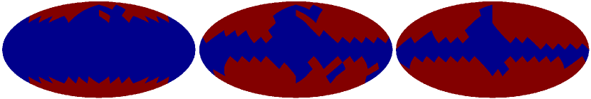
Figure 8: Conservative (left), fiducial (middle), and aggressive (right) masks used in this work, whose sky coverages are $f_{\rm fsky}=0.22$, $0.59$, and $0.69$, respectively.

Table 3: Limits on $r$ with different masks against the foreground model of one-component MBB dust and power-law synchrotron emissions with our case A configuration ($40,60,140,230,280,340$ GHz). The input tensor-to-scalar ratio is $r=0$.

mask	$f_{\rm sky}$	mean	limit (95% CL)
full-sky	1.0	$3.4\times 10^{-4}$	$<0.72\times 10^{-3}$
aggressive	0.69	$1.7\times 10^{-4}$	$<0.48\times 10^{-3}$
fiducial	0.59	$9.9\times 10^{-5}$	$<0.34\times 10^{-3}$
conservative	0.22	$7.7\times 10^{-5}$	$<0.52\times 10^{-3}$

References

- (1) M. Kamionkowski and E. D. Kovetz, ARA&A, 54, 227–269 (September 2016), 1510.06042.
- (2) BICEP2/Keck and Planck Collaborations, Phys. Rev. Lett., 114(10), 101301 (March 2015), 1502.00612.
- (3) S. M. Leach et al., A&A, 491, 597–615 (November 2008), 0805.0269.
- (4) M. Remazeilles et al., J. Cosmology Astropart. Phys, 4, 023 (April 2018), 1704.04501.
- (5) Planck Collaboration IV, ArXiv e-prints (July 2018), 1807.06208.
- (6) L. Page et al., ApJS, 170, 335–376 (June 2007), astro-ph/0603450.
- (7) G. Efstathiou, S. Gratton, and F. Paci, MNRAS, 397, 1355–1373 (August 2009), 0902.4803.
- (8) N. Katayama and E. Komatsu, ApJ, 737, 78 (August 2011), 1101.5210.
- (9) R. Fernández-Cobos, P. Vielva, R. B. Barreiro, and E. Martínez-González, MNRAS, 420, 2162–2169 (March 2012), arXiv:1106.2016.
- (10) R. Fernández-Cobos, A. Marcos-Caballero, P. Vielva, E. Martínez-González, and R. B. Barreiro, MNRAS, 459, 441–454 (June 2016), 1601.01515.
- (11) K. Ichiki, Progress of Theoretical and Experimental Physics, 2014(6), 06B109 (June 2014).
- (12) F. R. Bouchet and R. Gispert, New A, 4, 443–479 (September 1999), astro-ph/9903176.
- (13) R. Saha and P. K. Aluri, ApJ, 829, 113 (October 2016), 1509.03656.
- (14) Planck Collaboration XIII, A&A, 594, A13 (September 2016), 1502.01589.
- (15) K. M. Górski, E. Hivon, A. J. Banday, B. D. Wandelt, F. K. Hansen, M. Reinecke, and M. Bartelmann, ApJ, 622, 759–771 (April 2005), astro-ph/0409513.
- (16) H. Ishino et al., LiteBIRD: lite satellite for the study of B-mode polarization and inflation from cosmic microwave background radiation detection, In Space Telescopes and Instrumentation 2016: Optical, Infrared, and Millimeter Wave, volume 9904 of Proc. SPIE, page 99040X (July 2016).
- (17) H. K. Eriksen, G. Huey, R. Saha, F. K. Hansen, J. Dick, A. J. Banday, K. M. Górski, P. Jain, J. B. Jewell, L. Knox, D. L. Larson, I. J. O’Dwyer, T. Souradeep, and B. D. Wandelt, ApJ, 656, 641–652 (February 2007), astro-ph/0606088.
- (18) R. Stompor, S. Leach, F. Stivoli, and C. Baccigalupi, MNRAS, 392, 216–232 (January 2009), 0804.2645.
- (19) F. Vansyngel, B. D. Wandelt, J.-F. Cardoso, and K. Benabed, A&A, 588, A113 (April 2016), 1409.0858.
- (20) F. Vansyngel, The blind Bayesian approach to Cosmic Microwave Background data analysis, PhD thesis, Université Pierre et Marie Curie - Paris VI (December 2014).
- (21) Planck Collaboration X, A&A, 594, A10 (September 2016), 1502.01588.
- (22) M.-A. Miville-Deschênes, N. Ysard, A. Lavabre, N. Ponthieu, J. F. Macías-Pérez, J. Aumont, and J. P. Bernard, A&A, 490, 1093–1102 (November 2008), 0802.3345.
- (23) D. P. Finkbeiner, M. Davis, and D. J. Schlegel, ApJ, 524, 867–886 (October 1999), astro-ph/9905128.
- (24) A. M. Meisner and D. P. Finkbeiner, ApJ, 798, 88 (January 2015), 1410.7523.
- (25) G. Hinshaw et al., ApJS, 180, 225–245 (February 2009), arXiv:0803.0732.
- (26) K. Tassis and V. Pavlidou, MNRAS, 451, L90–L94 (July 2015), arXiv:1410.8136.
- (27) J. Poh and S. Dodelson, Phys. Rev. D, 95, 103511 (May 2017).
- (28) Planck Collaboration XI, ArXiv e-prints, page arXiv:1801.04945 (January 2018), arXiv:1801.04945.
- (29) J. Chluba, J. C. Hill, and M. H. Abitbol, MNRAS, 472, 1195–1213 (November 2017).
- (30) E. M. Leitch and A. C. R. Readhead, Advances in Astronomy, 2013, 352407 (2013).
- (31) C. Dickinson et al., New Astronomy Reviews, 80, 1–28 (February 2018).
- (32) C. L. Bennett et al., ApJS, 208, 20 (October 2013), 1212.5225.
- (33) Planck Collaboration XXV, A&A, 594, A25 (September 2016), 1506.06660.
- (34) R. Génova-Santos, J. A. Rubiño-Martín, A. Peláez-Santos, F. Poidevin, R. Rebolo, R. Vignaga, E. Artal, S. Harper, R. Hoyland, A. Lasenby, E. Martínez-González, L. Piccirillo, D. Tramonte, and R. A. Watson, MNRAS, 464, 4107–4132 (February 2017), 1605.04741.
- (35) M. Remazeilles, C. Dickinson, H. K. K. Eriksen, and I. K. Wehus, MNRAS, 458, 2032–2050 (May 2016), 1509.04714.
- (36) Y. Ali-Haïmoud, C. M. Hirata, and C. Dickinson, MNRAS, 395, 1055–1078 (May 2009), 0812.2904.
- (37) N. Krachmalnicoff, E. Carretti, C. Baccigalupi, G. Bernardi, S. Brown, B. M. Gaensler, M. Haverkorn, M. Kesteven, F. Perrotta, S. Poppi, and L. Staveley-Smith, ArXiv e-prints (February 2018), 1802.01145.