Multimodal Grounding for Sequence-to-Sequence Speech Recognition

Abstract

Humans are capable of processing speech by making use of multiple sensory modalities. For example, the environment where a conversation takes place generally provides semantic and/or acoustic context that helps us to resolve ambiguities or to recall named entities. Motivated by this, there have been many works studying the integration of visual information into the speech recognition pipeline. Specifically, in our previous work, we propose a multistep visual adaptive training approach which improves the accuracy of an audio-based Automatic Speech Recognition (ASR) system. This approach, however, is not end-to-end as it requires fine-tuning the whole model with an adaptation layer. In this paper, we propose novel end-to-end multimodal ASR systems and compare them to the adaptive approach by using a range of visual representations obtained from state-of-the-art convolutional neural networks. We show that adaptive training is effective for S2S models leading to an absolute improvement of 1.4% in word error rate. As for the end-to-end systems, although they perform better than baseline, the improvements are slightly less than adaptive training, 0.8 absolute WER reduction in single-best models. Using ensemble decoding, end-to-end models reach a WER of 15% which is the lowest score among all systems.

Index Terms—  Multimodal ASR, Deep learning

1 Introduction

Multimodal sensory integration is an important aspect of information processing and reasoning in human beings. Although deep neural networks (DNN) are more and more replacing the previous state-of-the-art approaches [1] in many fields of AI including machine translation, speech recognition and vision-related tasks; a structured way of fusioning multiple modalities still remains challenging.

In the context of automatic speech recognition (ASR), the presence of a synchronized video stream of the narrator enables lipreading [2] a technique to reduce the effect of ambient noise. This approach can be defined as a local grounding since the grounding happens between phonemes and visemes which are their visual counterparts. On the other hand, global grounding can always happen even the recognizer does not have access to the aforementioned synchronized video stream, i.e. when the video consistently provides object, action and scene level cues correlated with the speech content as may be the case with instructional videos. Here, visual cues from the recording environment (indoor vs outdoor) or the interaction between salient objects (people, instruments, vehicles, tools and equipments) can be exploited by the recognizer in various ways to learn a better acoustic and/or language model [3, 4, 5]. Figure 1 shows such an example where an ASR system without access to visual modality can produce an homophonic utterance like eucalylie instead of the rarely occurring correct word ukulele.

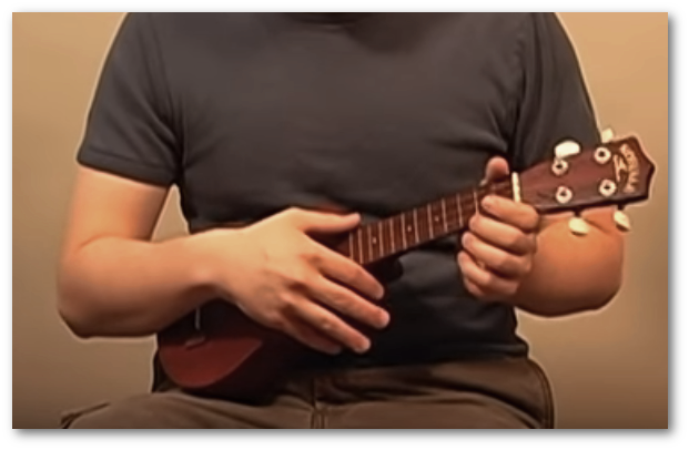
Fig. 1: An example ground-truth transcript which contains a rare visual word: “and that’s how you tune a ukulele”.

In this paper, we first apply an adaptive training scheme [3, 4, 5] for sequence-to-sequence (S2S) speech recognition and then propose two novel multimodal grounding methods for S2S ASR inspired from previous work in image captioning [6] and multimodal neural machine translation (MMT) [7, 8]. We compare both approaches through the use of visual features extracted from pre-trained models trained for object, scene and action recognition tasks [9, 10, 11]. We conduct all the experiments on How2 [12], a 300 hours collection of instructional videos. The main contributions of the paper can be summarized as follows: (1) a systematic evaluation reveals that the adaptive training is also effective for S2S models: we observe 1.4% absolute WER improvement with action-level features. (2) Although the proposed end-to-end multimodal systems improve upon the baseline ASR by around 0.5-0.8% absolute WER on average and for single-best respectively, they can not surpass the adaptive systems. (3) However, with ensemble-decoding these systems reach 15% WER leaving both the baseline and the adaptive systems behind.

2 Multimodal ASR Architectures

In the following, $\mathrm{X}\mathrm{=}\{x_{0},\dots,x_{T-1}\}$ represents an input sequence of $T$ speech features. The one-hot and continuous representation of a token is denoted by $\bar{y}\in\{0,1\}^{V}$ and $y$ respectively where $V$ is the vocabulary size. For multimodal models, $f$ is a visual feature vector associated to an utterance.

Our baseline model is a sequence-to-sequence architecture with attention [13]. The encoder is composed of 6 bidirectional LSTM layers [14], each followed by a tanh projection layer. The middle two LSTM layers apply a temporal subsampling [15] by skipping every other input, reducing the length of the sequence $\mathrm{X}$ from $T$ to $T/4$. All LSTM and projection layers have 320 hidden units. The forward-pass of the encoder produces the source encodings $\mathrm{E}$ of shape $(T/4)\times 320$ on top of which attention will be applied within the decoder. The hidden and cell states of all LSTM layers are initialized with $0$. The decoder is a 2-layer stacked GRU [16], where the first GRU receives the previous hidden state of the second GRU for all $t>0$. GRU layers, attention layer and embeddings have 320 hidden units. We share the input and output embeddings to reduce the number of parameters [17]. At timestep $t\mathrm{=}0$, the hidden state $h_{0}^{D_{1}}$ of GRU₁ is initialized with the average source encoding $e$ computed as follows:

$$e=\tfrac{1}{T/4}\sum_{t}\mathrm{E}_{t}\quad,\quad h_{0}^{D_{1}}=\text{tanh}\left(\mathbf{W_{h}}\ e\right)$$ (1)

A feed-forward attention mechanism [13] is used between the two GRU layers to compute the context vector $z_{t}$. GRU₂ receives $z_{t}$ as input and computes its next hidden state $h_{t}^{D_{2}}$. The output $o_{t}$ of the decoder which is used to estimate the probability distribution is a non-linear transformation of $h_{t}^{D_{2}}$:

$$h_{t}^{D_{1}} = \text{GRU}_{1}(y_{t-1},h_{t-1}^{D_{1}})$$ (2)

$$z_{t} = \text{AT}(\mathrm{E},h_{t}^{D_{1}})$$ (3)

$$h_{t}^{D_{2}} = \text{GRU}_{2}(z_{t},h_{t}^{D_{1}})$$ (4)

$$o_{t} = \mathbf{W}_{p}\,\text{tanh}(\mathbf{W}_{o}\,h_{t}^{D_{2}}+b_{o})+b_{p}$$ (5)

$$P(\bar{y}_{t}=j) = \text{softmax}(o_{t})_{j}$$ (6)

2.1 Visual Adaptive Training

Visual Adaptive Training (VAT) aims to fine-tune a pre-trained ASR model using visual modality. The pre-trained model may or may not be fully converged, the latter being the previously followed approach [5]. In this work, however, we preferred to use a converged ASR model. VAT adds a new linear layer to the ASR architecture to project the visual feature vector $f$ into the speech feature space (equation 7). The output of this layer, which is considered to be an utterance-specific shift vector, is then added to the speech features and the network is jointly optimized until convergence:

$$s =\mathbf{W_{v}}f+b_{v}$$ (7)

$$x_{t} =x_{t}+s\quad\quad\quad t\in\{0,\dots,T-1\}$$ (8)

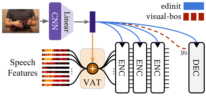
Fig. 2: Proposed architectures: VAT stands for visual adaptive training while edinit and visual-bos are end-to-end models.

2.2 Tied Initialization for Encoder & Decoder

Initializing the encoder and the decoder is an approach previously explored in multimodal machine translation [7, 8]. In order to ground the speech encoder with visual context, we first introduce two non-linear layers to learn an initial hidden and cell state globally for all LSTM layers $E_{k}$ in the encoder:

$$h_{0}^{E_{k}} =\text{tanh}\left(\mathbf{W_{h}}f+b_{h}\right)\quad k\in\{1,\dots,6\}$$ (9)

$$c_{0}^{E_{k}} =\text{tanh}\left(\mathbf{W_{c}}f+b_{c}\right)$$ (10)

The same idea can also be applied to initialize the GRU₁ in the decoder by replacing the equation 1 with the following:

$$h_{0}^{D_{1}}=\text{tanh}\left(\mathbf{W_{d}}f+b_{d}\right)$$ (11)

Finally we explore a third variant where we fuse the two approaches by sharing the linear layers in equations 9 and  11 i.e. by setting $\mathbf{W_{d}}\mathrm{=}\mathbf{W_{h}}$. In the following, these models will be referred to as einit, dinit and edinit respectively.

2.3 Visual Beginning-of-Sentence

Traditionally, neural decoders receive a special beginning of sentence <bos> vector as input at timestep $t\mathrm{=}0$ in order to initiate decoding. Depending on the implementation, this vector can be either constant or learned during training, the latter being the approach taken in this work. The disadvantage of both methods is the fact that during inference, the decoder always receives the same embedding at $t\mathrm{=}0$ regardless of what has been observed in the input of the network. Here we propose to modulate the decoder by replacing the static <bos> with a visually-informed one:

$$y_{0}^{i}=\mathbf{W_{v}}f^{i}+b_{v}$$ (12)

3 Dataset & Features

We conduct all experiments on the How2 dataset of instructional videos [12]. The official train, val and test splits consist of 185K, 2022 and 2305 sentences equivalent to 298, 3 and 4 hours of audio-visual stream respectively. We early-stop the training on val while model selection is performed on the test set. For preprocessing, we first lowercase and remove punctuations from the English transcripts and then train a SentencePiece model [18] to construct a subword vocabulary of 5000 tokens. We use Kaldi [19] to extract 40-dimensional filter bank features from 16kHz raw speech signal using a time window of 25ms and an overlap of 10ms. 3-dimensional pitch features are further concatenated to form the final feature vectors. A per-video mean and variance normalization is applied.

In the How2 dataset, a video is divided into smaller sentence-level clips and a clip is itself a sequence of consecutive frames. We first extract one frame per second from each clip, resize it and take a center crop of shape 224x224. We then explore two methods for producing a single feature vector for each clip belonging to a given video: (1) a per-clip representation by averaging feature vectors of frames of a clip and (2), a per-video representation which averages the feature vectors of all frames of a video. The latter ignores the variability among the clips of the same video by consistently representing its associated clips with the same feature. As for the types of features, we mainly explore three CNNs pre-trained on different visual tasks:

• Object-level. A ResNet-152 [9] trained on ImageNet [20] which consists of 1000 categories ranging from animals, flowers to devices and foods and so on.

• Action-level. A 3D ResNeXt-101 [11] trained on Kinetics dataset [21] which covers 400 categories such as eating, cooking, knitting and playing instruments.

• Scene-level. A ResNet-50 trained on Places365 [10] for scene recognition with 365 categories including but not limited to garden, valley,studio, theater and office.

For object and scene-level features, we extract 2048D average pooled (avgpool) convolutional features from the penultimate layer of the CNN as well as posterior class probabilities (prob) which are 1000D and 365D respectively. For the action-level CNN, we only experiment with 2048D per-video features.

4 Results

In all of the following experiments, we use ADAM [22] optimizer with a learning rate of 0.0004. The gradients are clipped to have unit norm. A dropout of 0.4 is applied on the final encoder and decoder outputs. The training is early stopped if validation WER does not improve for ten epochs. The learning rate is halved if WER does not improve for two epochs. We report average and ensemble scores of three independent runs. We decode hypotheses using a beam size of 10. The experiments are conducted using nmtpytorch [23].

	CNN	Avg. WER
		avgpool	prob
per-clips	objects	18.3	18.9
	scene	18.2	19.0
per-video	object	18.2	18.7
	scene	18.1	18.8
	action	18.0	-
Baseline		19.4
Restart		19.1

Table 1: Results for adaptive training experiments.

Visual Adaptive Training.

We report the results in Table 1. First, we clearly see that avgpool features consistently outperform class probability features. Similarly, a per-video representation for all clips of a given video seems to give a slight boost compared to per-clip granularity. In overall, adaptive training using avgpool features reduces the WER by up to 1.4 absolute points depending on the feature type and granularity. A secondary baseline restart which continues training the pre-trained ASR model without any adaptation layer is provided to show that the improvements obtained are not merely a side-effect of training the system for more time. However, we discover that when the adaptation layer is discarded during test time, the system still obtains around 18.0% WER. This may indicate that the effect of visual adaptation is indirect in the sense that it is actually making the ASR more robust.

End-to-End Variants.

For the initialization experiments, we observe that an exclusive initialization of either encoders or the decoder is not improving the results while the tied initialization obtains 0.8 and 0.5 absolute reduction in WER in terms of single-best and average results (Table 2). With ensembling, the edinit variant reaches the best WER (15.0%) among the models. The second approach visual-bos also performs similarly to the tied initialization. For both approaches, action-level features give slightly better performance.

Qualitative Examples.

Returning back to the initial example (Figure 1), we checked how successful the systems are when transcribing the word ukulele. We observe that edinit systems with action and object features could transcribe it once (out of ten occurrences in the test set) while the baseline system could not. However, this should be taken with a grain of salt as the token occurs only three times in the training set.

System	Feature	Min WER	Avg WER	Ens WER
baseline	-	19.2	19.4	15.6
dinit	action	19.2	19.4	15.5
einit	action	18.8	19.2	15.6
edinit	scene	18.8	19.2	15.4
edinit	object	18.5	18.9	15.2
edinit	action	18.4	18.9	15.0
visual-bos	object	19.0	19.1	15.5
visual-bos	scene	18.7	19.0	15.2
visual-bos	action	18.5	18.9	15.1

Table 2: Comparison of end-to-end systems: all features are 2048D avgpool per-video. Ens stands for ensemble decoding.

5 Related Work

During the last decade, the speech processing community proposed several acoustic model (AM) and language model (LM) based adaptation approaches using characteristics such as speaker or topic information [24, 25]. Miao et al. [24] proposes speaker-dependent training while Chen et al. [25] adapts a Recurrent Neural Network Language Model (RNNLM) using topic information. Although similar, our approach differs from these as the auxiliary information source is visual instead of being linguistic or acoustic.

Closely related to our work, Miao et al. [3] propose a visual adaptation strategy for AM in the context of hybrid HMM-DNN systems: they exploit the correlation between an utterance and the video content by using a feature vector extracted from a video frame. Similarly, Sun et al. [26], Gupta et al. [4], and Moriya et al. [27] explores the visual adaptation on language modeling side. Since we are dealing with end-to-end, sequence-to-sequence (S2S) architectures, we propose a global grounding instead of separate AM and LM adaptation in contrast to the aforementioned works. This also allows us to analyse and compare a plethora of adaptation and end-to-end training capabilities (section 4).

More related to our work, Palaskar et al. [5] evaluates the visual adaptive training [3] within the framework of Connectionist Temporal Classification (CTC) based ASR and also proposes an end-to-end scheme with feature concatenation for S2S models. Our work can be considered as an extension of [5] since we analyse the behaviour of adaptive training in S2S models for the first time. In addition, we propose novel end-to-end multimodal approaches namely the tied initialization of encoders and the decoder (section 2.2) inspired from previous work in multimodal machine translation [7, 8] and the visually informed decoding (section 2.3) similar to previous work in image captioning [6]. This latter is also explored in the context of RNNLM adaptation and rescoring by Moriya et al. [27]. Finally, we present a detailed analysis on the effect of different visual features on multimodal ASR performance.

6 Conclusions

In this paper, we first explored previously proposed visual adaptive training for S2S ASR models and then experimented with two novel end-to-end multimodal systems. Our experiments showed that visual adaptive training is effective for S2S models as well, reaching up to 1.4% absolute WER improvement for action-level features. However, we discovered that the adaptive system still preserves its performance even when the adaptation layer is discarded after training. We leave the analysis of this phenomenon to future work. Although end-to-end models perform better than the baseline, the difference is smaller compared to adaptive training, 0.8 absolute WER reduction in terms of single-best models. But when ensembling is used during decoding, the end-to-end models obtain the best WER (around 15%) among all models. With regard to the visual feature types, we show that average-pooled CNN features perform better than posterior probability features. We also observe that action-level features are consistently better than other features although the difference is not very large.

7 Acknowledgments

This work was started at JSALT 2018, and supported by JHU with gifts from Amazon, Facebook, Google, Microsoft & Mitsubishi Electric. It was also supported by the French National Research Agency (ANR) through the CHIST-ERA M2CR project under the contract ANR-15-CHR2-0006-01 and partly supported by DARPA grant FA8750-18-2-0018 under the AIDA program. This work used the Extreme Science and Engineering Discovery Environment (XSEDE) supported by NSF grant ACI-1548562 and the Bridges system supported by NSF award ACI-1445606, at the Pittsburgh Supercomputing Center.

References

- [1] Yann Lecun, Yoshua Bengio, and Geoffrey Hinton, “Deep learning,” Nature, vol. 521, no. 7553, pp. 436–444, 5 2015.
- [2] J. S. Chung, A. Senior, O. Vinyals, and A. Zisserman, “Lip reading sentences in the wild,” in IEEE Conference on Computer Vision and Pattern Recognition, 2017.
- [3] Yajie Miao and Florian Metze, “Open-domain audio-visual speech recognition: A deep learning approach,” in Interspeech 2016, 2016, pp. 3414–3418.
- [4] Abhinav Gupta, Yajie Miao, Leonardo Neves, and Florian Metze, “Visual features for context-aware speech recognition,” in 2017 IEEE International Conference on Acoustics, Speech and Signal Processing (ICASSP), March 2017, pp. 5020–5024.
- [5] Shruti Palaskar, Ramon Sanabria, and Florian Metze, “End-to-end multimodal speech recognition,” arXiv preprint arXiv:1804.09713, 2018.
- [6] Oriol Vinyals, Alexander Toshev, Samy Bengio, and Dumitru Erhan, “Show and tell: Lessons learned from the 2015 mscoco image captioning challenge,” IEEE Trans. Pattern Anal. Mach. Intell., vol. 39, no. 4, pp. 652–663, Apr. 2017.
- [7] Iacer Calixto and Qun Liu, “Incorporating global visual features into attention-based neural machine translation.,” in Proceedings of the 2017 Conference on Empirical Methods in Natural Language Processing, Copenhagen, Denmark, September 2017, pp. 992–1003, Association for Computational Linguistics.
- [8] Ozan Caglayan, Walid Aransa, Adrien Bardet, Mercedes García-Martínez, Fethi Bougares, Loïc Barrault, Marc Masana, Luis Herranz, and Joost van de Weijer, “LIUM-CVC submissions for WMT17 multimodal translation task,” in Proceedings of the Second Conference on Machine Translation, Volume 2: Shared Task Papers, Copenhagen, Denmark, September 2017, pp. 432–439, Association for Computational Linguistics.
- [9] K. He, X. Zhang, S. Ren, and J. Sun, “Deep residual learning for image recognition,” in 2016 IEEE Conference on Computer Vision and Pattern Recognition (CVPR), 2016, pp. 770–778.
- [10] Bolei Zhou, Agata Lapedriza, Aditya Khosla, Aude Oliva, and Antonio Torralba, “Places: A 10 million image database for scene recognition,” IEEE Transactions on Pattern Analysis and Machine Intelligence, 2017.
- [11] Kensho Hara, Hirokatsu Kataoka, and Yutaka Satoh, “Can spatiotemporal 3d cnns retrace the history of 2d cnns and imagenet?,” in Proceedings of the IEEE Conference on Computer Vision and Pattern Recognition (CVPR), 2018, pp. 6546–6555.
- [12] Ramon Sanabria, Ozan Caglayan, Shruti Palaskar, Desmond Elliott, Loïc Barrault, Lucia Specia, and Florian Metze, “How2: a large-scale dataset for multimodal language understanding,” in Proceedings of the Workshop on Visually Grounded Interaction and Language (ViGIL). NeurIPS, 2018.
- [13] Dzmitry Bahdanau, Kyunghyun Cho, and Yoshua Bengio, “Neural machine translation by jointly learning to align and translate,” CoRR, vol. abs/1409.0473, 2014.
- [14] Sepp Hochreiter and Jürgen Schmidhuber, “Long short-term memory,” Neural computation, vol. 9, no. 8, pp. 1735–1780, 1997.
- [15] W. Chan, N. Jaitly, Q. Le, and O. Vinyals, “Listen, attend and spell: A neural network for large vocabulary conversational speech recognition,” in 2016 IEEE International Conference on Acoustics, Speech and Signal Processing (ICASSP), March 2016, pp. 4960–4964.
- [16] Junyoung Chung, Çaglar Gülçehre, KyungHyun Cho, and Yoshua Bengio, “Empirical evaluation of gated recurrent neural networks on sequence modeling,” CoRR, vol. abs/1412.3555, 2014.
- [17] Ofir Press and Lior Wolf, “Using the output embedding to improve language models,” arXiv preprint arXiv:1608.05859, 2016.
- [18] Taku Kudo, “SentencePiece: A simple and language independent subword tokenizer and detokenizer for neural text processing,” in Proceedings of the 2018 Conference on Empirical Methods in Natural Language Processing, Brussels, Belgium, October 2018.
- [19] Daniel Povey, Arnab Ghoshal, Gilles Boulianne, Lukas Burget, Ondrej Glembek, Nagendra Goel, Mirko Hannemann, Petr Motlicek, Yanmin Qian, Petr Schwarz, Jan Silovsky, Georg Stemmer, and Karel Vesely, “The Kaldi speech recognition toolkit,” in Workshop on Automatic Speech Recognition and Understanding. IEEE, 2011.
- [20] Jia Deng, Wei Dong, Richard Socher, Li-Jia Li, Kai Li, and Li Fei-Fei, “Imagenet: A large-scale hierarchical image database,” in Computer Vision and Pattern Recognition, 2009. CVPR 2009. IEEE Conference on. IEEE, 2009, pp. 248–255.
- [21] Will Kay, Joao Carreira, Karen Simonyan, Brian Zhang, Chloe Hillier, Sudheendra Vijayanarasimhan, Fabio Viola, Tim Green, Trevor Back, Paul Natsev, et al., “The kinetics human action video dataset,” arXiv preprint arXiv:1705.06950, 2017.
- [22] Diederik Kingma and Jimmy Ba, “Adam: A method for stochastic optimization,” arXiv preprint arXiv:1412.6980, 2014.
- [23] Ozan Caglayan, Mercedes García-Martínez, Adrien Bardet, Walid Aransa, Fethi Bougares, and Loïc Barrault, “Nmtpy: A flexible toolkit for advanced neural machine translation systems,” Prague Bull. Math. Linguistics, vol. 109, pp. 15–28, 2017.
- [24] Yajie Miao, Hao Zhang, and Florian Metze, “Speaker adaptive training of deep neural network acoustic models using i-vectors,” IEEE/ACM Transactions on Audio, Speech and Language Processing (TASLP), vol. 23, no. 11, pp. 1938–1949, 2015.
- [25] Xie Chen, Tian Tan, Xunying Liu, Pierre Lanchantin, Moquan Wan, Mark JF Gales, and Philip C Woodland, “Recurrent neural network language model adaptation for multi-genre broadcast speech recognition,” in Sixteenth Annual Conference of the International Speech Communication Association, 2015.
- [26] Felix Sun, David Harwath, and James Glass, “Look, listen, and decode: Multimodal speech recognition with images,” in Spoken Language Technology Workshop (SLT). IEEE, 2016, pp. 573–578.
- [27] Yasufumi Moriya and Gareth J. F. Jones, “LSTM language model adaptation with images and titles for multimedia automatic speech recognition,” in Spoken Language Technology Workshop (SLT). IEEE, 2018.