Limit of p-Laplacian Obstacle problems

Abstract.

In this paper we study asymptotic behavior of solutions to obstacle problems for $p-$Laplacians as $p\to\infty.$ For the one-dimensional case and for the radial case, we give an explicit expression of the limit. In the n-dimensional case, we provide sufficient conditions to assure the uniform convergence of whole family of the solutions of obstacle problems either for data $f$ that change sign in $\Omega$ or for data $f$ (that do not change sign in $\Omega$) possibly vanishing in a set of positive measure.

Keywords: p-Laplace equations, $\infty$-Laplace equations, asymptotic behaviour, obstacle problems.

AMS 35J60, 35J65, 35B30, 35J87

1. Introduction

The study of obstacle problems for both $p$-Laplacian and $\infty$-Laplacian, which has recently received a strong impulse, is closely connected with many relevant topics such as the mass optimization problems, the Absolutely Minimizing Lipschitz Extensions, the Infinity Harmonic Functions, the Monge-Kantorovich mass transfer problem and the Tug of War Games. We mention for instance [1], [2], [3], [4], [5], [10], [12], [15], [16], [17], [18], [19], [21], and the references therein.

In this paper we study the asymptotic behavior of solutions to obstacle problems for $p-$Laplacians as $p$ tends to $\infty.$ Let $\Omega\subset\mathbb{R}^{n}$ denote a bounded domain. We consider the problem:

$$\text{find }u\in\mathcal{K},\,\,\,\,\int_{\Omega}|\nabla u|^{p-2}\nabla u\nabla(v-u)\,dx\,-\int_{\Omega}f(v-u)\,dx\,\geqslant 0\,\,\,\forall v\in\mathcal{K},$$ (1.1)

where

$$\mathcal{K}=\{v\in W_{0}^{1,p}(\Omega):\ v\geqslant\varphi\,\text{in}\,\,\Omega\,\}$$

with obstacle $\varphi\in W^{1,p}(\Omega),$ $\varphi\leq 0$ on $\partial\Omega,$ and the datum

$$f\in L^{\infty}(\Omega).$$ (1.2)

Then, for any fixed $p,$ there exists a unique solution $u_{p}.$ If we assume

$$-\triangle_{p}\varphi\in L^{p^{\prime}}(\Omega),$$ (1.3)

where $-\triangle_{p}u=-div(|\nabla u|^{p-2}\nabla u),$ then the following Lewy-Stampacchia inequality holds (see [20])

$$f\leq-\triangle_{p}u_{p}\leq-\triangle_{p}\varphi\vee f.$$ (1.4)

Moreover, see for instance [18] and Theorem 3.1 in [7], if

$$\mathcal{K}^{\infty}=\{u\in W_{0}^{1,\infty}(\Omega):u\geqslant\varphi\ \text{ in }\Omega,||\nabla u||_{L^{\infty}(\Omega)}\leq 1\}\neq\emptyset$$ (1.5)

then the family of the solution $u_{p}$ is pre-compact in $C(\bar{\Omega});$ in particular, from any sequence $u_{p_{k}}$ we can extract a subsequence $u_{{p_{k}}_{j}}$ converging to a function $u_{\infty}$ in $C(\bar{\Omega})$, $u_{\infty}$ being a maximizer of the following problem:

$$\mathcal{F}(u)=\max\biggl{\{}\mathcal{F}(w):w\in\mathcal{K}^{\infty}\biggl{\}}$$ (1.6)

where

$$\mathcal{F}(w)=\int_{\Omega}w(x)f(x)dx.$$

Moreover,

$$\limsup_{p\to\infty}||\nabla u_{p}||_{L^{\infty}(\Omega)}\leq 1.$$ (1.7)

The limit Problem (1.6) is related to an optimal mass transport problem with taxes. More precisely, in [18] it is proved that solutions to obstacle problems for $p-$Laplacians give an approximation to the extra production/demand necessary in the process and to a Kantorovich potential for the corresponding transport problem. Moreover, in [18], the authors also show that this problem can be interpreted as an optimal mass transport problem with courier.

In this paper we face the question whether the whole family of the solutions $u_{p}$ of the obstacle Problem (1.1) is convergent to the same limit function $u_{\infty}.$ For the analogous results for Dirichlet problems we mention [3], [5], [10], [11], [13], and the references therein. The asymptotic behavior of minimizers of $p$-energy forms on fractals as the Sierpinski Gasket (as $p\to\infty$) has been recently addressed in [6].

In the present paper, we give an explicit expression of the limit for the one-dimensional case and for the radial case (see Theorems 3.1 and 4.1). For arbitrary $n-$dimensional domains, we provide sufficient conditions to assure the uniform convergence of whole family of the solutions to obstacle problems either for data $f$ that change sign in $\Omega$ or for data $f$ (that do not change sign in $\Omega$) possibly vanishing in a set of positive measure (see Theorems 4.2, 4.3, 4.4, 4.5 and 4.6). Our paper has been deeply inspired by Ishii and Loreti, [13], nevertheless the obstacle problems present their own peculiarities and structural difficulties. In Remarks 3.3, 5.3, 5.1, 5.5 and 5.6 we highlight some peculiarities. The main difficulties are due to the fact that the solution $u_{p}$ to Problem 1.1 satisfies the equation only on the set where it is detached from the obstacle. As this set depends on $p$ then we have to deal with Dirichlet problems with non homogeneous boundary conditions in intervals moving with $p$ (see Theorem 2.1, Proposition 2.2 and Remark 2.2). Hence the behavior of coincidence sets $\Gamma_{p}$ (3.1) plays a crucial role (see condition (3.2)). As the regularity properties of the free boundaries are important tools for the study of the behavior of coincidence sets, then our approach is strictly related to the papers [19] and [4]. In particular Theorem 2.8 in [19] as well as Theorems 7.5 and 1.3 in [4] provide sufficient conditions to assure that condition (3.2) holds. We note that in [19] and [4] smoothness assumptions are required while in our paper we deal with a larger class of obstacles and data. In Section 5 we give examples of obstacle problems where condition (3.2) is satisfied even if neither the assumptions of Theorem 2.8 in [19] nor those of Theorem 7.5 in [4] are satisfied. We note that hypothesis (3.2) is not assumed in Theorems 4.2, 4.3, 4.4 and 4.5. In Theorem 4.2 concerning data $f$ changing sign in $\Omega,$ condition (4.14) puts in relation the position of the support of $f$ with respect to the boundary of $\Omega$ and it provides an alternative assumption that, in some sense, forces the coincidence sets to have a good behavior. Similarly the sign conditions on the datum $f$ in Theorems 4.3 and 4.4 provide alternative assumptions. Furthermore we remark that, as the constraint in the convex $\mathcal{K}$ is from below, then as a consequence of the Lewy-Stampacchia inequality (1.4), the easy situation is when $f$ (possibly vanishing in a set of positive measure) is non negative while, when $f$ is non positive, we have to require also conditions on $-\triangle_{p}\varphi$ (see (4.26) and (4.28) respectively). Finally, in Section 5 we give some examples of non trivial obstacle problems where all the assumptions of Theorem 4.6 are satisfied (see Examples 2 and 5).

As mentioned above, our topic is intrinsically related to the Absolutely Minimizing Lipschitz Extensions (AMLEs), to viscosity solutions to the obstacle problem for the $\infty$-Laplacian and to comparison principles for $\infty-$superharmonic functions (see [15] and [19]). To prove Theorems 4.2, 4.3, 4.4, 4.5 and 4.6 we use such approaches and tools. More precisely, under suitable assumptions, every sequence of solutions $u_{p}$ to obstacle problems (1.1), being viscosity solutions (with respect to the $p$-Laplacian), converges to a viscosity solution $u_{\infty}$ of the obstacle problem for the $\infty$-Laplacian, which is the smallest continuous $\infty-$superharmonic function above the obstacle. Hence the limit $u_{\infty}$ is unique. In fact, among the solutions to Problem (1.6) the limit $u_{\infty}$ is the (unique) Absolutely Minimizing Lipschitz Extension (AMLE) according to the terminology of [2] (see Example 6 in Section 5). In [19] the authors consider obstacle problems for both the $\infty$-Laplacian and the $p$-Laplacians (see also [4] for similar results). Theorems 4.2, 4.3, 4.4, 4.5, and 4.6 refer to a more general class of problems and require weaker assumptions than the ones in [19] (see Section 4). Moreover Theorems 3.1 and 4.1 provide, for the limit of solutions $u_{p},$ a simple representation in terms of the data. We note that the proofs of Theorems 3.1 and 4.1 do not involve the deep, delicate theory of viscosity solutions for $\infty$-Laplacian and AMLE solutions.

The plan of the paper is the following. Section 2 concerns one-dimensional Dirichlet problems with non homogeneous boundary data, Section 3 concerns the one-dimensional obstacle problem. In Section 4 we consider the n-dimensional case. In the last section we provide examples, comments and remarks.

2. One-dimensional Dirichlet problem with non homogeneous boundary data

We consider Dirichlet problems with non homogeneous boundary data in the one-dimensional case. More precisely, we consider the following problem on $\Omega=(a,b),$

$$\text{find }u\in\mathcal{K}_{D},\,\,\,\,\int_{\Omega}|\nabla u|^{p-2}\nabla u\nabla v\,dx\,=\int_{\Omega}fv\,dx\\ ,\,\,\forall v\in W_{0}^{1,p}(\Omega),$$ (2.1)

where

$$\mathcal{K}_{D}=\{u\in W^{1,p}(\Omega):u(a)=A_{p},u(b)=B_{p}\}.$$

For any fixed $p,$ and $f\in L^{\infty}(\Omega)$ there exists a unique solution $u_{p}.$ By proceeding as in [13], we can prove that, if

$$\frac{|B_{p}-A_{p}|}{b-a}\leq 1,\qquad A_{p}\to A,\qquad B_{p}\to B,$$ (2.2)

then $u_{p}\longrightarrow u_{\infty}$ weakly in $W^{1,m}(\Omega),\forall m>2$, $u_{\infty}$ being a maximizer of the following variational problem

$$\int_{\Omega}u_{\infty}(x)f(x)dx=\max\biggl{\{}\mathcal{F}(w):w\in\mathcal{K}_{D}^{\infty}\biggl{\}}$$ (2.3)

where

$$\mathcal{F}(w)=\int_{\Omega}w(x)f(x)dx$$

$$\mathcal{K}_{D}^{\infty}=\{u\in W^{1,\infty}(\Omega):u(a)=A,u(b)=B,||\nabla u||_{L^{\infty}(\Omega)}\leq 1\}.$$

From now on we denote by $\mu(E)$ the $n$-dimensional Lebesgue measure of the set $E\subset\mathbb{R}^{n}.$

More precisely, the following theorem holds.

Theorem 2.1.

Suppose that (1.2) and (2.2) hold. Then $u_{p}$ converges uniformly to the following function $U\in\mathcal{K}_{D}^{\infty}:$

$$U(x)=\int_{a}^{x}(\chi_{O_{-}}-\chi_{O_{+}}+k\chi_{O_{0}})dt+A$$ (2.4)

where

$$O_{-}=\{x\in(a,b),F<\beta^{*}\},\quad\quad O_{+}=\{x\in(a,b),F>\beta^{*}\},\quad\quad O_{0}=\{x\in(a,b),F=\beta^{*}\}$$

$$F(x)=\int_{a}^{x}f(t)dt,\quad\quad h(r)=\mu(\{x\in\Omega:F(x)<r\})$$

$$\beta^{*}=\sup\{r\in\mathbb{R}:h(r)\leq\frac{b-a-A+B}{2}\}\,$$ (2.5)

and

$$k=\begin{cases}\frac{\mu(O_{+})-\mu(O_{-})-A+B}{\mu(O_{0})}\qquad if\qquad\mu(O_{0})>0,\\ 0\qquad if\qquad\mu(O_{0})=0.\\ \end{cases}$$ (2.6)

We skip the proof, as it is similar to the proof of following Theorem 3.1.

Remark 2.1.

If

$$\frac{|B_{p}-A_{p}|}{b-a}\geq 1$$ (2.7)

the solution (2.4) does not depend on the datum $f.$

More precisely, we have the following proposition.

Proposition 2.1.

If

$$\frac{|B_{p}-A_{p}|}{b-a}\geq 1,\qquad A_{p}\to A,\qquad B_{p}\to B$$ (2.8)

then

$$U(x)=A+(\frac{B-A}{b-a})(x-a).$$ (2.9)

Proof.

First we consider $\frac{|B_{p}-A_{p}|}{b-a}=1$ and $A>B.$ Then

$$\beta^{*}=\sup\{r\in\mathbb{R},h(r)\leq 0\}$$ (2.10)

and then $\beta^{*}=F_{-}=\min_{x\in[a,b]}F(x).$ So $O_{-}=\emptyset$ and if $\mu(O_{o})>0$, then $k=-1$ (see (2.6)) and (2.9) is proved.

If $\frac{|B_{p}-A_{p}|}{b-a}=1$ holds and $A<B,$ then $\beta^{*}=\sup\{r\in\mathbb{R}:h(r)\leq b-a\}=+\infty$ and then $O_{+}=O_{0}=\emptyset$ and $O_{-}=(a,b)$ and (2.9) is showed.

If $\frac{|B_{p}-A_{p}|}{b-a}=D_{p}>1$ holds, we consider $u_{p}=D_{p}v_{p}$ where $v_{p}$ solve

$$-\frac{d}{dx}(|u^{\prime}(x)|^{p-2}u^{\prime}(x))=\frac{f(x)}{D^{p-1}_{p}}$$ (2.11)

with $v_{p}(a)=A_{p}/D_{p},$ $v_{p}(b)=B_{p}/D_{p}$ and

$$\frac{|B_{p}-A_{p}|}{D_{p}(b-a)}=1.$$ (2.12)

Then $v_{p}$ converges to

$$V(x)=\frac{1}{D}(A+(\frac{B-A}{b-a})(x-a))$$

where $D=\frac{|B-A|}{b-a}$ and then (2.9) is proved. ∎

We note that the result of Theorem 2.1 holds also for a family of Dirichlet problems in moving intervals. More precisely, consider the problems on $\Omega_{p}=(a_{p},b_{p}),$ $f\in L^{\infty}(\Omega)$

$$\begin{cases}\text{find }u_{p}\in W^{1,p}(\Omega_{p})\,\,\text{such that}\,\,u_{p}(a_{p})=A_{p},\,\,u_{p}(b_{p})=B_{p},\text{and}\\ \int_{\Omega_{p}}|\nabla u|^{p-2}\nabla u\nabla v\,dx\,=\int_{\Omega_{p}}fv\,dx\,\,\,\forall v\in W_{0}^{1,p}(\Omega_{p}).\end{cases}$$ (2.13)

Then the following proposition holds (we skip the proof, as it is similar to the proof of Theorem 3.1).

Proposition 2.2.

Suppose

$$\frac{|B_{p}-A_{p}|}{b_{p}-a_{p}}\leq 1,\,\,\text{and}\,\,A_{p}\to A,\,\,B_{p}\to B,\quad a_{p}\to a,\,\,b_{p}\to b,\quad a_{p}\geq a,\,\,\quad b_{p}\leq b.$$ (2.14)

Then the solution $u_{p}$ converges (locally) uniformly in $(a,b)$ to the function $U$ defined in (2.4).

Remark 2.2.

From the previous proposition we deduce that for any choice of family of points $x_{p}\in[a,b),\,x_{p}\to\eta\in[a,b)$ and of points $y_{p}\in(a,b],\,\,y_{p}>x_{p},\,\,\,y_{p}\to\gamma\in(a,b]$ with $\eta<\gamma$ the solutions $v_{p}$ of Problems (2.13) in the intervals $(x_{p},y_{p})$ converges (locally) uniformly in $(\eta,\gamma)$ to the restriction to the interval $(\eta,\gamma)$ of the function $U$ defined in (2.4).

3. One-dimensional Obstacle problem

We consider the obstacle problem (1.1) on $\Omega=(a,b).$

We define the closed set

$$\Gamma_{p}=\{x\in\bar{\Omega}:u_{p}=\varphi\};$$ (3.1)

we set

$$\Gamma_{\infty}=\liminf\Gamma_{p}\quad\text{and }\qquad\Gamma^{*}_{\infty}=\limsup\Gamma_{p},$$

and we recall that

$$\limsup\Gamma_{p}=\cap^{\infty}_{p=1}\cup_{n\geq p}\Gamma_{n}\,\text{and }\liminf\Gamma_{p}=\cup^{\infty}_{p=1}\cap_{n\geq p}\Gamma_{n}$$

and we simply write $\lim\Gamma_{p}$ if $\Gamma_{\infty}=\Gamma^{*}_{\infty}$ (for the definition of $\limsup\Gamma_{p}$ and of $\liminf\Gamma_{p}$ we refer to [14]).

Theorem 3.1.

We assume hypotheses (1.2), (1.3), (1.5) and

$$\overline{int\Gamma_{\infty}^{*}}\subset\Gamma_{\infty}.$$ (3.2)

Then the solution $u_{p}$ converges uniformly to the following function $U\in\mathcal{K}^{\infty}:$

$$U=\varphi\,\,\text{in}\,\,\Gamma_{\infty}$$

and for any (connected) component $(d,e),$ $[d,e]\subset(a,b)$ of $\Omega\setminus\Gamma_{\infty}$

$$U(x)=\int_{d}^{x}(\chi_{O_{-}}-\chi_{O_{+}}+k\chi_{O_{0}})dt+\varphi(d)$$ (3.3)

where

$$O_{-}=\{x\in(d,e),F<\beta^{*}\},\quad\quad O_{+}=\{x\in(d,e),F>\beta^{*}\},\quad\quad O_{0}=\{x\in(d,e),F=\beta^{*}\}$$

$$F(x)=\int_{d}^{x}f(t)dt,\quad\quad h(r)=\mu(\{x\in(d,e):F(x)<r\})$$ (3.4)

$$\beta^{*}=\sup\{r\in\mathbb{R}:h(r)\leq\frac{e-d-\varphi(d)+\varphi(e)}{2}\}\,$$ (3.5)

$$k=\begin{cases}\frac{\mu(O_{+})-\mu(O_{-})-\varphi(d)+\varphi(e)}{\mu(O_{0})}&\qquad if\qquad\mu(O_{0})>0,\\ 0&\qquad if\qquad\mu(O_{0})=0.\\ \end{cases}$$ (3.6)

For any (connected) component $(a,c)$ of $\Omega\setminus\Gamma_{\infty}$

$$U(x)=\int_{a}^{x}(\chi_{O_{-}}-\chi_{O_{+}}+k\chi_{O_{0}})dt$$ (3.7)

where

$$O_{-}=\{x\in(a,c),F<\beta^{*}\},\quad\quad O_{+}=\{x\in(a,c),F>\beta^{*}\},\quad\quad O_{0}=\{x\in(a,c),F=\beta^{*}\}$$

$$F(x)=\int_{a}^{x}f(t)dt,\quad\quad h(r)=\mu(\{x\in(a,c):F(x)<r\})$$

$$\beta^{*}=\sup\{r\in\mathbb{R}:h(r)\leq\frac{c-a+\varphi(c)}{2}\}\,$$ (3.8)

$$k=\begin{cases}\frac{\mu(O_{+})-\mu(O_{-})+\varphi(c)}{\mu(O_{0})}\qquad&if\qquad\mu(O_{0})>0,\\ 0\qquad&if\qquad\mu(O_{0})=0.\\ \end{cases}$$ (3.9)

For any (connected) component $(d,b)$ of $\Omega\setminus\Gamma_{\infty}$

$$U(x)=\int_{b}^{x}(\chi_{O_{-}}-\chi_{O_{+}}+k\chi_{O_{0}})dt$$ (3.10)

where

$$O_{-}=\{x\in(d,b),F<\beta^{*}\},\quad\quad O_{+}=\{x\in(d,b),F>\beta^{*}\},\quad\quad O_{0}=\{x\in(d,b),F=\beta^{*}\}$$

$$F(x)=\int_{b}^{x}f(t)dt,\quad\quad h(r)=\mu(\{x\in(d,b):F(x)<r\})$$

$$\beta^{*}=\sup\{r\in\mathbb{R}:h(r)\leq\frac{b-d-\varphi(d)}{2}\}\,$$ (3.11)

$$k=\begin{cases}\frac{\mu(O_{+})-\mu(O_{-})-\varphi(d)}{\mu(O_{0})}\qquad&if\qquad\mu(O_{0})>0,\\ 0\qquad&if\qquad\mu(O_{0})=0.\\ \end{cases}$$ (3.12)

From now on we denote by $Lip_{1}(\bar{\Omega})$ the space of the Lipschitz functions with Lipschitz constant less or equal to $1.$

Remark 3.1.

We note that if $\varphi\leq 0$ on $\partial\Omega,$ then the assumption $\varphi\in Lip_{1}(\bar{\Omega})$ implies that the convex $\mathcal{K}^{\infty}$ is not empty but this condition is not necessary. In fact, on $\Omega=(-2,2),$ the obstacle $\varphi=1-x^{2}$ does not belong to the space $Lip_{1}(\bar{\Omega})$ while assumption (1.5) is satisfied as the following function $w$ belongs to $\mathcal{K}^{\infty}$

$$w=\begin{cases}0\qquad&-2<x\leq-\frac{5}{4}\\ x+\frac{5}{4}\qquad&-\frac{5}{4}<x\leq-\frac{1}{2}\\ 1-x^{2}\qquad&-\frac{1}{2}<x\leq\frac{1}{2}\\ -x+\frac{5}{4}\qquad&\frac{1}{2}<x\leq\frac{5}{4}\\ 0\qquad&\frac{5}{4}<x\leq 2\end{cases}$$

(see Section 5).

Before proving Theorem 3.1, we establish the following preliminary results which take into account the three different cases for the connected components of $\Omega\setminus\Gamma_{\infty}.$

Proposition 3.1.

Let $x_{p}\in(a,b)$ and $y_{p}\in(x_{p},b)$ such that $-\triangle u_{p}=f$ in $(x_{p},y_{p}),$ $u_{p}(x_{p})=\varphi(x_{p}),$ $u_{p}(y_{p})=\varphi(y_{p}).$ If

$$\frac{|u_{p}(y_{p})-u_{p}(x_{p})|}{y_{p}-x_{p}}\leq 1,$$ (3.13)

then there exists a unique value of $\beta$, say $\beta_{p},$ such that

$$u_{p}(y_{p})=u_{p}(x_{p})+\int_{x_{p}}^{y_{p}}\psi_{p}(\beta_{p}-F_{p}^{**}(t))dt$$

where $\psi_{p}(s)=|s|^{\frac{1}{p-1}-1}s$ for $s\in\mathbb{R}$ and $F_{p}^{**}(x)=\int_{x_{p}}^{x}f(t)dt.$

Moreover,

$$\beta_{p}\in[F_{-,p}-1,F_{+,p}+1]\quad\,\,\text{where}\quad\,\ F_{+,p}=\max_{[x_{p},y_{p}]}F_{p}^{**},\qquad F_{-,p}=\min_{[x_{p},y_{p}]}F_{p}^{**}.$$ (3.14)

Proof.

We recall that the solution $u_{p}$ belongs to $C^{1}([a,b])$ (see (1.2), (1.3) and (1.4)).

According to [13], we obtain that for any $x\in(x_{p},y_{p})$

$$u_{p}(x)=u_{p}(x_{p})+\int_{x_{p}}^{x}\psi_{p}(\beta_{p}-F_{p}^{**}(t))dt$$ (3.15)

with $\psi_{p}(s)=|s|^{\frac{1}{p-1}-1}s$ for $s\in\mathbb{R},$ $F_{p}^{**}(x)=\int_{x_{p}}^{x}f(t)dt$ and

$$\beta_{p}=|u^{\prime}_{p}(x_{p})|^{p-2}u^{\prime}_{p}(x_{p}).$$ (3.16)

By the property of $\psi_{p},$ there exists a unique value of $\beta$, say $\beta_{p},$ such that

$$u_{p}(y_{p})=u_{p}(x_{p})+\int_{x_{p}}^{y_{p}}\psi_{p}(\beta_{p}-F_{p}^{**}(t))dt.$$

We observe that

$$\beta_{p}\in[F_{-,p}-1,F_{+,p}+1]$$ (3.17)

where $F_{+,p}$ and $F_{-,p}$ are defined in (3.14).

We verify that

$$\int_{x_{p}}^{y_{p}}\psi_{p}(F_{+,p}+1-F_{p}^{**}(t))dt\geq u_{p}(y_{p})-u_{p}(x_{p}).$$

If $u_{p}(y_{p})-u_{p}(x_{p})\leq 0,$ the previous inequality holds trivially. Suppose $u_{p}(y_{p})-u_{p}(x_{p})>0,$ then

$$(F_{+,p}+1-F_{p}^{**}(t))\geq(\frac{u_{p}(y_{p})-u_{p}(x_{p})}{y_{p}-x_{p}})^{p-1}$$

where we use (3.13).

Now we verify that

$$\int_{x_{p}}^{y_{p}}\psi_{p}(F_{-,p}-1-F_{p}^{**}(t))dt\leq u_{p}(y_{p})-u_{p}(x_{p}).$$

If $u_{p}(y_{p})-u_{p}(x_{p})\geq 0,$ the previous inequality holds trivially. Suppose $u_{p}(y_{p})-u_{p}(x_{p})<0,$ then

$$(-F_{-,p}+1+F_{p}^{**}(t))\geq(\frac{u_{p}(x_{p})-u_{p}(y_{p})}{y_{p}-x_{p}})^{p-1}$$

where we use (3.13). ∎

By proceeding as in the proof of Proposition 3.1 we can show the following result that concerns the second case.

Proposition 3.2.

Let $x_{p}\in(a,b),$ such that $-\triangle u_{p}=f$ in $(a,x_{p}),$ $u_{p}(x_{p})=\varphi(x_{p}),\,u_{p}(a)=0.$

If

$$\frac{|u_{p}(x_{p})-u_{p}(a)|}{x_{p}-a}\leq 1$$ (3.18)

then there exists a unique value of $\beta$, say $\beta_{p},$ such that

$$u_{p}(x_{p})=\int_{a}^{x_{p}}\psi_{p}(\beta_{p}-F(t))dt$$

where $\psi_{p}(s)=|s|^{\frac{1}{p-1}-1}s$ for $s\in\mathbb{R}$ and $F(x)=\int_{a}^{x}f(t)dt.$

Moreover, $\beta_{p}\in[\hat{F}_{-}-1,\hat{F}_{+}+1]$ where

$$\hat{F}_{+}=\min_{[a,x_{p}]}F\qquad\hat{F}_{-}=\min_{[a,x_{p}]}F.$$ (3.19)

For the last case in Theorem 3.1 we establish the following result that can be proved as Proposition 3.1.

Proposition 3.3.

Let $x_{p}\in(a,b)$ such that $-\triangle_{p}u_{p}=f$ in $(x_{p},b),$ $u_{p}(x_{p})=\varphi(x_{p}),$ $u_{p}(b)=0.$ If

$$\frac{|u_{p}(b)-u_{p}(x_{p})|}{b-x_{p}}\leq 1,$$ (3.20)

then there exists a unique value of $\beta$, say $\beta_{p},$ such that

$$u_{p}(x_{p})=-\int_{x_{p}}^{b}\psi_{p}(\beta_{p}+F^{*}(t))dt$$

where $\psi_{p}(s)=|s|^{\frac{1}{p-1}-1}s$ for $s\in\mathbb{R}$ and $F^{*}(x)=\int_{x}^{b}f(t)dt.$

Moreover,

$$\beta_{p}\in[T_{-}-1,T_{+}+1]\quad\text{where }T_{+}=\max_{[x_{p},b]}(-F^{*}(x)),\quad T_{-}=\min_{[x_{p},b]}(-F^{*}(x)).$$ (3.21)

Now we prove Theorem 3.1.

Proof.

We split the proof in 4 steps.

Step 1. Let the interval $(d,e)$ is a (connected) component of $\Omega\setminus\Gamma_{\infty}$ such that $[d,e]\subset(a,b)$ and we assume that

$$\begin{cases}\text{there exist }x_{p}>a,\,\text{ and }y_{p}\in(x_{p},b)\,\,\text{such that}\,\,-\triangle_{p}u_{p}=f\quad in\quad(x_{p},y_{p}),\\ u_{p}(x_{p})=\varphi(x_{p}),\,\,\,u_{p}(y_{p})=\varphi(y_{p}),\,\,\,\ x_{p}\to d,\,\,y_{p}\to e\end{cases}$$ (3.22)

and

$$\frac{|u_{p}(y_{p})-u_{p}(x_{p})|}{y_{p}-x_{p}}\leq 1$$ (3.23)

By Proposition 3.1 there exists a unique value of $\beta$, say $\beta_{p}\in[F_{-,p}-1,F_{+,p}+1],$ such that

$$u_{p}(y_{p})=u_{p}(x_{p})+\int_{x_{p}}^{y_{p}}\psi_{p}(\beta_{p}-F_{p}^{**}(t))dt$$

where $\psi_{p}(s)=|s|^{\frac{1}{p-1}-1}s$ for $s\in\mathbb{R}$ and $F_{p}^{**}(x)=\int_{x_{p}}^{x}f(t)dt.$ Moreover $F_{-,p}\to F_{-,d},$ $F_{+,p}\to F_{+,d},$ where

$$F_{+,d}=\max_{[d,e]}F\qquad F_{-,d}=\min_{[d,e]}F$$ (3.24)

and $F$ is defined in (3.4). We note that $F_{+,p}\leq F_{+}-F_{-}$ and $F_{-,p}\geq-F_{+}+F_{-}$ where

$$F_{+}=\max_{[a,b]}\int_{a}^{x}f(t)dt\qquad F_{-}=\min_{[a,b]}\int_{a}^{x}f(t)dt.$$ (3.25)

We set $\delta(F)=2(F_{+}+1-F_{-}).$ According to Formula (iv) on page 419, Lemma 3.2 and 3.3 in [13], the following properties hold:

1 $\lim_{t\to r^{-}}h(t)=h(r)\leq\mu(\{x\in(d,e):F(x)\leq r\})=\lim_{t\to r^{+}}h(r),$ $F$ defined in (3.4);

2 $h(r)$ is strictly increasing in $[F_{-,d},F_{+,d}];$

3 for $\beta\in[F_{-,p}-1,F_{+,p}+1],$

$$|\psi_{p}(\beta-F_{p}^{**}(x))|\leq\psi_{p}(\delta(F))\leq\psi_{1}(\delta(F));$$

4 let $\alpha_{j}\in[F_{-,p}-1,F_{+,p}+1]$ be a sequence converging to some $r\in\mathbb{R}$ and let $p_{j}$ be a sequence such that $p_{j}\to\infty.$ Then, for any $\phi\in L^{1}(\Omega),$

$$\int_{O_{-}(r)}\phi\,\psi_{p_{j}}(\alpha_{j}-F_{p_{j}}^{**}(x))dx\to\int_{O_{-}(r)}\phi\,dx$$

$$\int_{O_{+}(r)}\phi\,\psi_{p_{j}}(\alpha_{j}-F_{p_{j}}^{**}(x))dx\to-\int_{O_{+}(r)}\phi\,dx$$

with $O_{-}(r)=\{x\in(d,e),F<r\}$ and $O_{+}(r)=\{x\in(d,e),F>r\}.$

In fact let $x\in O_{-}(r)$ then $r-F(x)=\delta_{0}>0$ there exist a positive constant $\delta$ and an index $j_{0}$ such that for any $j\geq j_{0}$

$$\delta\leq\alpha_{j}-F_{p_{j}}^{**}(x)\leq\delta(F)$$

and so

$$\psi_{p_{j}}(\alpha_{j}-F_{p_{j}}^{**}(x))\to 1.$$

By property 3 and the Lebesgue convergence we obtain the first limit. If $x\in O_{+}(r)$ then $r-F(x)=-\delta_{0}<0$ there exist a positive constant $\delta$ and an index $j_{0}$ such that for any $j\geq j_{0}$

$$-\delta(F)\leq\alpha_{j}-F_{p_{j}}^{**}(x)\leq-\delta$$

and so

$$\psi_{p_{j}}(\alpha_{j}-F_{p_{j}}^{**}(x))\to 1.$$

By property 3 and the Lebesgue convergence we obtain the second limit. From (3.23), we deduce

$$\frac{|\varphi(d)-\varphi(e)|}{e-d}\leq 1.$$

First we suppose that

$$\varphi(d)-\varphi(e)>d-e$$ (3.26)

and we deduce that $\beta^{*}\leq F_{+,d}.$ In fact if $\beta^{*}>F_{+,d}$, then $h(\beta^{*})=e-d$ which contradicts the inequality $h(\beta^{*})\leq\frac{e-d-\varphi(d)+\varphi(e)}{2}<e-d$ that follows from definition (3.5).

Now we show that

$$\lim_{p\to\infty}\beta_{p}=\beta^{*}.$$

First we prove that

$$\liminf_{p\to\infty}\beta_{p}\geq\beta^{*}.$$ (3.27)

By contradiction we suppose that there exists a sequence $p_{j}\to\infty$ such that $\liminf_{p\to\infty}\beta_{p}=r<\beta^{*}.$ From the strictly monotonicity we have

$$\lim_{t\to r^{+}}h(t)<h(\beta^{*})\leq\frac{e-d-\varphi(d)+\varphi(e)}{2}.$$

Let $H=\{x\in(d,e),F\leq r\}$ and $L=\{x\in(d,e),F>r\}.$ Then we have

$$\lim_{t\to r^{+}}h(t)=\mu(H)<\frac{e-d-\varphi(d)+\varphi(e)}{2}$$

(see property 1) and

$$\mu(L)=e-d-\mu(H)>e-d-\frac{e-d-\varphi(d)+\varphi(e)}{2}=\frac{e-d+\varphi(d)-\varphi(e)}{2}.$$

By property 3, we obtain

$$\limsup_{j\to\infty}|\int_{H}\psi_{p_{j}}(\beta_{p_{j}}-F_{p_{j}}^{**}(x))dx|\leq\limsup_{j\to\infty}\int_{H}\psi_{p_{j}}(\delta(F))dx=\mu(H)<\frac{e-d-\varphi(d)+\varphi(e)}{2}.$$

By property 4, we obtain

$$\lim_{j\to\infty}\int_{L}\psi_{p_{j}}(\beta_{p_{j}}-F_{p_{j}}^{**}(x))dx=-\mu(L)<-\frac{e-d-\varphi(d)+\varphi(e)}{2}.$$

As

$$u_{p_{j}}(y_{p_{j}})-u_{p_{j}}(x_{p_{j}})=\int_{x_{p_{j}}}^{y_{p_{j}}}\psi_{p_{j}}(\beta_{p_{j}}-F_{p_{j}}^{**}(x))dx$$

passing to the limit for $j\to\infty$ we obtain

$$\limsup_{j\to\infty}(u_{p_{j}}(y_{p_{j}})-u_{p_{j}}(x_{p_{j}}))<\varphi(e)-\varphi(d)$$

and that is a contradiction. In fact

$$\limsup_{j\to\infty}(\varphi(e)-u_{p_{j}}(x_{p_{j}}))\leq\limsup_{j\to\infty}(u_{p_{j}}(y_{p_{j}})-u_{p_{j}}(x_{p_{j}}))<\varphi(e)-\varphi(d)$$

that is

$$\liminf_{j\to\infty}u_{{p_{j}}}(x_{p_{j}})=\liminf_{j\to\infty}\varphi(x_{p_{j}})>\varphi(d)$$

as $u_{p}(x_{p})=\varphi(x_{p}),$ $u_{p}(y_{p})=\varphi(y_{p})$ and $x_{p}\to d,$ $y_{p}\to e$ by (3.22).

Now we prove that

$$\limsup_{p\to\infty}\beta_{p}\leq\beta^{*}.$$

Again by contradiction we suppose that there exists a sequence $p_{j}\to\infty$ such that $\limsup_{p\to\infty}\beta_{p}=r>\beta^{*}.$

Let $H=\{x\in(d,e),F\geq r\}$ and $L=\{x\in(d,e),F<r\}.$ Then we have

$$\mu(L)>\frac{e-d-\varphi(d)+\varphi(e)}{2}$$

(see property 1) and

$$\mu(H)=e-d-\mu(L)<e-d-\frac{e-d-\varphi(d)+\varphi(e)}{2}=\frac{e-d+\varphi(d)-\varphi(e)}{2}.$$

By property 3, we obtain

$$\liminf_{j\to\infty}\int_{H}\psi_{p_{j}}(\beta_{p_{j}}-F_{p_{j}}^{**}(x))dx\geq-\mu(H)>-\frac{e-d+\varphi(d)-\varphi(e)}{2}.$$

By property 4, we obtain

$$\lim_{j\to\infty}\int_{L}\psi_{p_{j}}(\beta_{p_{j}}-F_{p_{j}}^{**}(x))dx=\mu(L)>\frac{e-d-\varphi(d)+\varphi(e)}{2}.$$

As

$$u_{p_{j}}(y_{p_{j}})-u_{p_{j}}(x_{p_{j}})=\int_{x_{p_{j}}}^{y_{p_{j}}}\psi_{p_{j}}(\beta_{p_{j}}-F_{p_{j}}^{**}(x))dx,$$

passing to the limit for $j\to\infty,$ we obtain

$$\liminf_{j\to\infty}(u_{p_{j}}(y_{p_{j}})-u_{p_{j}}(x_{p_{j}}))>\varphi(e)-\varphi(d)$$

$$\liminf_{j\to\infty}u_{p_{j}}(y_{p_{j}})-\varphi(d)\geq\liminf_{j\to\infty}(u_{p_{j}}(y_{p_{j}})-u_{p_{j}}(x_{p_{j}}))>\varphi(e)-\varphi(d)$$

$$\liminf_{j\to\infty}u_{p_{j}}(y_{p_{j}})-\varphi(e)>0$$

and this fact is a contradiction.

Now we prove that $|k|\leq 1$ where $k$ is defined in (3.6). Let $[d,e]\subset\Omega.$ By property 1 ($e-d=\mu(O_{0})+\mu(O_{-})+\mu(O_{+})$)

$$\mu(O_{-})=h(\beta^{*})\leq\frac{e-d-\varphi(d)+\varphi(e)}{2}\leq\lim_{t\to(\beta^{*})^{+}}h(t)=\mu(O_{0})+\mu(O_{-}):$$

then

$$0\geq 2\mu(O_{-})-(e-d-\varphi(d)+\varphi(e))=\mu(O_{-})-\mu(O_{0})-\mu(O_{+})-(-\varphi(d)+\varphi(e)),$$

that is,

$$-\mu(O_{0})\leq-\mu(O_{-})+\mu(O_{+})+(-\varphi(d)+\varphi(e))$$

and

$$0\leq 2\mu(O_{0})+2\mu(O_{-})-(e-d-\varphi(d)+\varphi(e))=\mu(O_{0})+\mu(O_{-})-\mu(O_{+})-(-\varphi(d)+\varphi(e)),$$

that is,

$$\mu(O_{0})\geq-\mu(O_{-})+\mu(O_{+})+(-\varphi(d)+\varphi(e)).$$

Then, if $\mu(O_{0})>0$

$$-1\leq k=\frac{\mu(O_{+})-\mu(O_{-})-\varphi(d)+\varphi(e)}{\mu(O_{0})}\leq 1.$$ (3.28)

Now we prove that if $\mu(O_{0})>0$ then

$$\lim_{p\to\infty}\psi_{p}(\beta_{p}-\beta^{*})=k.$$ (3.29)

In fact, we have

$$u_{p}(y_{p})-u_{p}(x_{p})=\int_{x_{p}}^{y_{p}}\psi_{p}(\beta_{p}-F_{p}^{**}(x))dx=\int_{x_{p}}^{d}\psi_{p}(\beta_{p}-F_{p}^{**}(x))dx+\int_{e}^{y_{p}}\psi_{p}(\beta_{p}-F_{p}^{**}(x))dx+$$

$$\int_{O_{-}}\psi_{p}(\beta_{p}-F_{p}^{**}(t))dt+\int_{O_{+}}\psi_{p}(\beta_{p}-F_{p}^{**}(t))dt+\psi_{p}(\beta_{p}-\beta^{*}-\int_{d}^{x_{p}}fdt)\mu(O_{0}).$$

As $u_{p}(x_{p})=\varphi(x_{p}),$ $u_{p}(y_{p})=\varphi(y_{p})$ and $x_{p}\to d,$ $y_{p}\to e$ by (3.22), by property 4, we obtain

$$\lim_{p\to\infty}(\varphi(y_{p})-\varphi(x_{p}))=\mu(O_{-})-\mu(O_{+})+\lim_{p\to\infty}\psi_{p}(\beta_{p}-\beta^{*}-\int_{d}^{x_{p}}fdt)\mu(O_{0})$$

and (3.29) is proved.

For any $x\in(d,e)$ we have, by (3.22), that $x\in(x_{p},y_{p})$ (for $p\geq p_{0}),$ and, by (3.15),

$$u_{p}(x)=\varphi(x_{p})+\int_{x_{p}}^{x}\psi_{p}(\beta_{p}-F_{p}^{**}(t))dt=\int_{x_{p}}^{d}\psi_{p}(\beta_{p}-F_{p}^{**}(x))dx+$$

$$\int^{x}_{d}\chi_{O_{-}}\psi_{p}(\beta_{p}-F_{p}^{**}(t))dt+\int^{x}_{d}\chi_{O_{+}}\psi_{p}(\beta_{p}-F_{p}^{**}(t))dt+\psi_{p}(\beta_{p}-\beta^{*}-\int_{d}^{x_{p}}fdt)\mu(O_{0}).$$

By property 4 and (3.29), passing to the limit,

$$\lim_{p\to\infty}u_{p}(x)=\varphi(d)-\int_{d}^{x}\chi_{O_{+}}dt+\int_{d}^{x}\chi_{O_{-}}dt+k\int_{d}^{x}\chi_{O_{0}}dt$$ (3.30)

and we obtain (3.3).

To complete the proof of the theorem we have to consider the case $\varphi(d)-\varphi(e)=d-e.$ If $\varphi(d)-\varphi(e)=d-e$ then

$$\beta^{*}=\sup\{r\in\mathbb{R}:h(r)\leq d-e\}=+\infty$$

and then $O_{+}=O_{0}=\emptyset$ and $O_{-}=(d,e).$

By proceeding as in the proof of (3.27) we show that

$$r=\liminf_{p\to\infty}\beta_{p}\geq F_{+,d}.$$ (3.31)

Let the sequence $p_{j}\to\infty$ be such that $\lim_{j\to\infty}\,\beta_{p_{j}}=r\geq F_{+,d}$ and denote by $O_{-}(r)=\{x\in(d,e),F<r\},\,\,O_{0}(r)=\{x\in(d,e),F=r\}$ and $O_{+}(r)=\{x\in(d,e),F>r\}$ then $O_{+}(r)=\emptyset.$ We discuss first the case $r=F_{+,d}$

We proceed as in the proof of (3.28) to show that if $\mu(O_{0}(F_{+,d}))>0$ then $k=1$ where

$$\,\,\,k=\begin{cases}\frac{-\mu(O_{-}(F_{+,d}))-\varphi(d)+\varphi(e)}{\mu(O_{0}(F_{+,d}))}\qquad&if\qquad\mu(O_{0}(F_{+,d}))>0,\\ 0\qquad&if\qquad\mu(O_{0}(F_{+,d}))=0.\end{cases}$$ (3.32)

Analogously we proceed as in the proof of (3.29) and of (3.30) to show that if $\mu(O_{0}(F_{+,d}))>0$ then

$$\lim_{j\to\infty}\psi_{p_{j}}(\beta_{p_{j}}-F_{+,d})=1$$ (3.33)

and

$$\lim_{j\to\infty}u_{p_{j}}(x)=\varphi(d)+\int_{d}^{x}\chi_{O_{-}(F_{+,d})}dt+\int_{d}^{x}\chi_{O_{0}(F_{+,d})}dt=\varphi(d)+x-d$$

and (3.3) is proved.

Finally for any sequence $p_{j}\to\infty$ be such that $\lim_{j\to\infty}\,\beta_{p_{j}}=r^{*}>F_{+,d}$ we have $O_{+}(r^{*})=O_{0}(r^{*})=\emptyset,\,\,\,O_{-}(r^{*})=(d,e),\,\,\,k=0$ and

$$\lim_{j\to\infty}u_{p_{j}}(x)=\varphi(d)+x-d$$

and (3.3) is proved.

Step 2. We remove assumption (3.23). We start by noticing that, if (3.23) does not hold, by property (1.7) we deduce that

$$\limsup\frac{|u_{p}(y_{p})-u_{p}(x_{p})|}{y_{p}-x_{p}}=1$$

as $p\to\infty.$ Actually there exists the limit (see 3.22)

$$\lim\frac{|u_{p}(y_{p})-u_{p}(x_{p})|}{y_{p}-x_{p}}=\lim\frac{|\varphi(y_{p})-\varphi(x_{p})|}{y_{p}-x_{p}}=\frac{|\varphi(e)-\varphi(d)|}{e-d}=1.$$

According to Remark 2.2, Theorem 2.1 and Proposition 2.1, the limit function $U(x)$ is the affine function connecting the points $(d,\varphi(d))$ and $(e,\varphi(e))$ (see formula (2.9)) which coincides with the function defined in (3.3).

Step 3. We discuss assumption (3.22). As the interval $(d,e)$ is a (connected) component of $\Omega\setminus\Gamma_{\infty}$ (and $[d,e]\subset(a,b)$) by the definition of $\Gamma_{\infty}$ there exist $x_{p}\in(a,b)$ and $y^{*}_{p}\in(a,b)$ such that $x_{p}<y^{*}_{p},$     $u_{p}(x_{p})=\varphi(x_{p})$ and $x_{p}\to d,$ $u_{p}(y^{*}_{p})=\varphi(y^{*}_{p})$ and $y^{*}_{p}\to e.$ We discuss now the property

$$-\triangle_{p}u_{p}=f\,\,\text{in}\,\,(x_{p},y_{p}).$$ (3.34)

Let $z_{p}$ the first point $z_{p}\in(x_{p},y^{*}_{p})$ such that $u_{p}$ meets the obstacle i.e. $u_{p}(z_{p})=\varphi(z_{p}).$ First we note that $\limsup z_{p}\leq\lim y^{*}_{p}=e$ and $\liminf z_{p}\geq\lim x_{p}=d$ hence if $\liminf z_{p}=e$ then $z_{p}\to e,$ property (3.34) holds in the interval $(x_{p},z_{p})$ and we choose $y_{p}=z_{p}$.

Furthermore if there exists a sequence $z_{p_{j}}$ converging to some $\eta\in(d,e)$ such that $u_{p_{j}}(x)=\varphi(x),\,\,\forall x\in[z_{p_{j}},z_{p_{j}}+\delta_{p_{j}}],\,\,\delta_{p_{j}}>0$ then by assumption (3.2) we deduce that $\limsup\delta_{p_{j}}=0.$ In fact if $\limsup\delta_{p_{j}}=\delta_{0}>0$ then there exists $\delta>0$ such that the interval $[\eta,\eta+\delta]$ is contained in $\overline{int\Gamma_{\infty}^{*}}\bigcap(d,e)$ and this is a contradiction with the fact that $(d,e)\bigcap\Gamma_{\infty}=\emptyset.$ If $\limsup\delta_{p_{j}}=0$ then the interval $[z_{p_{j}},z_{p_{j}}+\delta_{p_{j}}]$ vanishes and the limit function $U(x)$ is not affected by these vanishing contacts (see Remark 2.2).

If $\eta=d$ the interval $[x_{p_{j}},z_{p_{j}}]$ vanishes and the limit function $U(x)$ is not affected by these vanishing contacts (see Remark 2.2). Similar arguments hold for the choice of the points $x_{p}.$

Step 4. If the interval $(a,c)$ is a (connected) component of $\Omega\setminus\Gamma_{\infty}$ we proceed in a similar manner using Proposition 3.2. If the interval $(d,b)$ is a (connected) component of $\Omega\setminus\Gamma_{\infty}$ we proceed in a similar manner using Proposition 3.3. ∎

Remark 3.2.

We note that a theorem analogous of Theorem 3.1 holds for obstacle problems with non homogeneous boundary conditions. We skip the proof, which can be easily done by modifying the proof of Theorem 3.1 and taking into account the results of Section 2 concerning the Dirichlet problem with non homogeneous boundary conditions.

Remark 3.3.

We note a peculiarity of the limit of solutions to obstacle Problems (1.1). If the right hand term in the Lewy-Stampacchia inequality (1.4) is uniformly bounded, then (up to pass to a subsequence) there exists the weak limit $f^{*}$ of the functions $-\bigtriangleup_{p}u_{p}.$ However the limit $U^{*}$ of the solutions $u_{p}^{*}$ of Dirichlet Problems (2.1) with datum $f^{*}$ may not coincide with the limit of the solutions to obstacle Problems (1.1). We can construct examples in which $U^{*}$ belongs to the convex $\mathcal{K}^{\infty}$ but it is not a maximizer of (1.6) (Example 2 in Section 5 ) as well as examples in which $U^{*}$ does not belongs to the convex (Example 1 in Section 5).

4. $n$-dimensional Obstacle problem

First we consider the radial case.

Let $\Omega$ be the annulus $B_{r_{1},r_{2}}:=\{x\in\mathbb{R}^{n},r_{1}<|x|<r_{2}\},$ $0<r_{1}<r_{2},$

$$f(x)=g(|x|)\quad\text{and}\quad\varphi(x)=\Phi(|x|).$$ (4.1)

Theorem 4.1.

Suppose that (1.2), (1.3), (1.5), (3.2) and (4.1) hold. Then the solutions $u_{p}$ of Problems (1.1) converge uniformly to the following function $U\in\mathcal{K}^{\infty}:$

$$U(x)=\varphi(x)\,\text{in}\,\,\Gamma_{\infty}$$

and for any (connected) component $B_{d,e}$ of $\Omega\setminus\Gamma_{\infty}$ such that $[d,e]\subset(r_{1},r_{2})$

$$U(x)=\int_{d}^{|x|}(\chi_{O_{-}}-\chi_{O_{+}}+k\chi_{O_{0}})dt+\Phi(d)$$ (4.2)

where

$$O_{-}=\{t\in(d,e),G<\beta^{*}\},\quad\quad O_{+}=\{t\in(d,e),G>\beta^{*}\},\quad\quad O_{0}=\{t\in(d,e),G=\beta^{*}\}$$

$$G(t)=\int_{d}^{t}\tau^{n-1}g(\tau)d\tau,\quad\quad h(r)=\mu(\{t\in(d,e):G(t)<r\})$$

$$\beta^{*}=\sup\{r\in\mathbb{R}:h(r)\leq\frac{e-d-\Phi(d)+\Phi(e)}{2}\}\,$$ (4.3)

$$k=\begin{cases}\frac{\mu(O_{+})-\mu(O_{-})-\Phi(d)+\Phi(e)}{\mu(O_{0})}\qquad if\qquad\mu(O_{0})>0,\\ 0\qquad if\qquad\mu(O_{0})=0.\\ \end{cases}$$ (4.4)

For any (connected) component $B_{r_{1},c}$ of $\Omega\setminus\Gamma_{\infty}$

$$U(x)=\int_{r_{1}}^{|x|}(\chi_{O_{-}}-\chi_{O_{+}}+k\chi_{O_{0}})dt$$ (4.5)

where

$$O_{-}=\{t\in(r_{1},c),G<\beta^{*}\},\quad\quad O_{+}=\{t\in(r_{1},c),G>\beta^{*}\},\quad\quad O_{0}=\{t\in(r_{1},c),G=\beta^{*}\}$$

$$G(t)=\int_{r_{1}}^{t}\tau^{n-1}g(\tau)d\tau,\quad\quad h(r)=\mu(\{t\in(r_{1},c):G(t)<r\})$$

$$\beta^{*}=\sup\{r\in\mathbb{R}:h(r)\leq\frac{c-r_{1}+\Phi(c)}{2}\}\,$$ (4.6)

$$k=\begin{cases}\frac{\mu(O_{+})-\mu(O_{-})+\Phi(c)}{\mu(O_{0})}\qquad if\qquad\mu(O_{0})>0,\\ 0\qquad if\qquad\mu(O_{0})=0.\\ \end{cases}$$ (4.7)

For any (connected) component $B_{d,r_{2}}$ of $\Omega\setminus\Gamma_{\infty}$

$$U(x)=\int_{r_{2}}^{|x|}(\chi_{O_{-}}-\chi_{O_{+}}+k\chi_{O_{0}})dt$$ (4.8)

where

$$O_{-}=\{t\in(d,r_{2}),G<\beta^{*}\},\quad\quad O_{+}=\{t\in(d,r_{2}),G>\beta^{*}\},\quad\quad O_{0}=\{t\in(d,r_{2}),F=\beta^{*}\}$$

$$G(t)=\int_{r_{2}}^{t}\tau^{n-1}g(\tau)d\tau,\quad\quad h(r)=\mu(\{t\in(d,r_{2}):G(t)<r\})$$

$$\beta^{*}=\sup\{r\in\mathbb{R}:h(r)\leq\frac{r_{2}-d-\Phi(d)}{2}\}\,$$ (4.9)

$$k=\begin{cases}\frac{\mu(O_{+})-\mu(O_{-})-\Phi(d)}{\mu(O_{0})}\qquad if\qquad\mu(O_{0})>0,\\ 0\qquad if\qquad\mu(O_{0})=0.\\ \end{cases}$$ (4.10)

We skip the proof, as it is very similar to the proof of Theorem 3.1. We note that in the previous results the solutions $u_{p}$ converge uniformly to the function $U$ as $p\to\infty$ even if Problem $\eqref{eq:3DV}$ does not have unique solution.

Remark 4.1.

If $\Omega$ is the ball $B_{r}:=\{x\in\mathbb{R}^{n},|x|<r\},$ $r>0,$ then under the assumptions of Theorem 4.1, the same results hold except for the case of the (connected) component $B_{0,c}$ of $\Omega\setminus\Gamma_{\infty}$ where formula (4.5) becomes

$$U(x)=\int_{c}^{|x|}(\chi_{O_{-}}-\chi_{O_{+}})dt+\Phi(c)$$ (4.11)

where

$$O_{-}=\{t\in(0,c),G<0\},\quad\quad O_{+}=\{t\in(0,c),G>0\},$$

$$G(t)=\int_{0}^{t}\tau^{n-1}g(\tau)d\tau.$$

The following results concern arbitrary domains hence as we do not assume any smoothness condition on the boundaries these results hold true for bad domains as the Koch Islands (see [7], [9] and [8]).

We denote

$$\mathcal{M}_{\varphi}=\{u\in\mathcal{K}^{\infty}:\mathcal{F}(u)=\max_{w\in\mathcal{K}^{\infty}}\mathcal{F}(w)\}$$

and

$$\mathcal{A}_{\varphi}=\{u\in C(\bar{\Omega}):\text{there exists a sequence}\,\,p_{j}\to\infty\quad\text{such that}\,\,u_{p_{j}}\to u\quad\text{in}\quad C(\bar{\Omega})\}$$ (4.12)

where $u_{p}$ denotes the solution to $(\ref{OPp})$.

Condition (3.2) is satisfied in all the examples of Section 5 and Theorem 2.8 in [19] as well as Theorems 7.5 and 1.3 in [4] provide sufficient conditions to assure that condition (3.2) holds true. However in [19] and [4] smoothness assumptions are required while in our paper we deal with a larger class of obstacles and data. Then we are interested in proving that the set $\mathcal{A}_{\varphi}$ defined in (4.12) is a singleton by a different approach (see Theorems 4.2, 4.3, 4.4 and 4.5). Condition (4.14) in Theorem 4.2, that concerns data $f$ changing sign in $\Omega,$ puts in relation the position of the support of $f$ with respect to the boundary of $\Omega$ and provides an alternative assumption that, in some sense, forces the coincidence sets to have a good behavior. Similarly, the sign conditions on the datum $f$ in Theorems 4.3, 4.4 provide alternative assumptions. Finally, we recall that, as the constraint in the convex $\mathcal{K}$ is from below, then as a consequence of the Lewy-Stampacchia inequality (1.4), the easy situation is when $f$ (possibly vanishing in a set of positive measure) is non negative while, when $f$ is non positive, we have to require also conditions on $-\triangle_{p}\varphi$ (see (4.26) and (4.28) respectively).

Theorem 4.2.

Suppose that (1.2), (1.3) and (1.5) hold, and

$$\Omega_{+}\quad\text{and}\quad\Omega_{-}\,\text{are open connected and non empty}$$ (4.13)

where

$$\Omega_{+}=\{x\in\Omega,f(x)>0\}\quad\text{and}\quad\Omega_{-}=\{x\in\Omega,f(x)<0\}$$

and

$$\inf_{x\in\Omega_{+}}\sup_{y\in\Omega_{-}}(d(x)+d(y)-|x-y|)\leq 0$$ (4.14)

where $d(x)$ denotes the distance of $x$ from the boundary. Then the set $\mathcal{A}_{\varphi}$ defined in (4.12) is a singleton.

We just observed $\mathcal{A}_{\varphi}\subset\mathcal{M}_{\varphi}$ and before proving this theorem, we state same preliminary results.

Proposition 4.1.

Let $u\in\mathcal{M}_{\varphi}$ then

$$u(x)=\inf\{u(y)+|x-y|,y\in\Omega_{-}\cup\partial\Omega\},\forall x\in\Omega$$ (4.15)

$$u(x)=\sup\{u(y)-|x-y|,y\in\Omega_{+}\cup\partial\Omega\}\vee\varphi^{*}(x),\forall x\in\Omega$$ (4.16)

where

$$\varphi^{*}(x)=\sup\{\varphi(y)-|x-y|,y\in\Omega\}.$$

Proof.

We prove (4.16), as (4.15) is similar (see Proposition 6.1 in [13]). Let

$$w(x)=\sup\{u(y)-|x-y|,y\in\Omega_{+}\cup\partial\Omega\}\vee\varphi^{*}(x).$$

As $u\in Lip_{1}(\bar{\Omega})$ and $u\geq\varphi$ we deduce $u\geq w.$ Moreover $w\in Lip_{1}(\bar{\Omega}),$ $u=w$ on $\Omega_{+}\cup\partial\Omega$ and $w\in\mathcal{K}^{\infty}.$ Then as

$$\int_{\Omega_{+}}fwdx+\int_{\Omega_{-}}fwdx=\mathcal{F}(w)\leq\mathcal{F}(u)=\int_{\Omega_{+}}fudx+\int_{\Omega_{-}}fudx$$

we obtain

$$\int_{\Omega_{-}}f(u-w)dx\geq 0$$

and so $u=w$ on $\Omega_{-}.$

∎

By proceeding as in the proof Propositions 6.4, 6.5, 6.6 and 6.7 of [13] we obtain la following result.

Proposition 4.2.

For any $u,v\in\mathcal{M}_{\varphi}$ we have

$$\sup_{\Omega_{+}}(u-v)^{+}=\sup_{\Omega_{-}}(u-v)^{+}$$ (4.17)

and

$$\nabla u=\nabla v\qquad\text{a. e. in }\Omega_{+}$$ (4.18)

Now we prove Theorem 4.2.

Proof.

First we show, that for any functions $u,v\in\mathcal{M}_{\varphi}$

$$u=v\,\text{on }suppf.$$ (4.19)

By contradiction we suppose $\sup_{\Omega_{+}}(u-v)^{+}=h>0$ then by (4.18) we obtain that $u(x)=v(x)+h$ for any $x\in\Omega_{+}.$

By (4.14), we deduce that for any $\varepsilon>0$, there exists a point $x_{\varepsilon}$ in $\Omega_{+}$ such that

$$d(x_{\varepsilon})+d(y)-|x_{\varepsilon}-y|\leq\varepsilon$$

for any $y\in\Omega_{-}.$ By using that $u,v\in Lip_{1}(\bar{\Omega})$ vanish on the boundary $\partial\Omega$ and property (4.15), we deduce

$$u(x_{\varepsilon})\leq d(x_{\varepsilon})\leq\varepsilon+v(x_{\varepsilon})$$

and this is a contradiction if $\varepsilon\in(0,h).$ Then $u(x)=v(x)$ for any $x\in\Omega_{+}.$ By (4.17) we deduce that $u(x)\leq v(x)$ for any $x\in\Omega_{-}.$ By changing the role of $u$ and $v$ in (4.17) we obtain $v(x)\leq u(x)$ for any $x\in\Omega_{-}$ and this completes the proof of (4.19).

Now, according to [19], for any $u\in\mathcal{A}_{\varphi}$ we denote by $\Gamma_{u}=\{x\in\Omega\setminus suppf:u(x)=\varphi(x)\}$ then

$$\begin{cases}u(x)\geq\varphi(x),&\quad\text{in}\quad\Omega\setminus suppf\\ -\triangle_{\infty}u=0&\quad\text{in}\quad\Omega\setminus(suppf\bigcup\Gamma_{u})\quad\text{in the viscosity sense}\\ -\triangle_{\infty}u\geq 0&\quad\text{in}\quad\Omega\setminus suppf\quad\text{in the viscosity sense}.\end{cases}$$ (4.20)

Now we denote by

$$w(x)=\inf\{v(x):v\in\mathcal{G}\}$$

where $\mathcal{G}$ denotes the set of the continuous functions that are infinity super-harmonic in $\Omega\setminus suppf$ and satisfy the conditions $v(x)\geq\varphi(x),\quad\text{in}\quad\Omega\setminus suppf$ and $v=u$ on $\partial(\Omega\setminus suppf).$ We note that $u\in\mathcal{G}$ and $w$ is upper semicontinuous and infinity super-harmonic in $\Omega\setminus suppf.$ Moreover $u\geq w.$

We consider the open set

$$W=\{x\in\Omega\setminus suppf:u(x)>w(x)\}.$$

We have $u(x)=w(x)$ on $\partial W$ and $u(x)>w(x)\geq\varphi$ in $W$ so $W\subset\Omega\setminus(suppf\bigcup\Gamma_{u})$ then $u$ is infinity harmonic in $W.$ By the comparison principle (see for instance [15]) we conclude that $u\leq w$ in $W.$ Hence $W=\emptyset$ and $u=w$ in $\Omega\setminus suppf.$

Moreover any element $v\in\mathcal{A}_{\varphi}$ belongs to $\mathcal{G}$ as $u=v=0$ on $\partial\Omega$ and by (4.19) we have $u=v$ on $suppf,$ hence $u\leq v.$ By the same argument we can show that $v\leq u$ then $u=v$ on $\Omega\setminus suppf.$ This completes the proof. ∎

We now discuss the situation in which the datum $f$ does not change sign in $\Omega.$ We note that $f(x)\geq\delta_{0}>0$ then $\mathcal{A}_{\varphi}=\{d(x)\}$ and in particular the set $\mathcal{A}_{\varphi}$ is a singleton. In fact we consider the Dirichlet problem:

$$\text{find }u\in W_{0}^{1,p}(\Omega),\,\,\,\,\int_{\Omega}|\nabla u|^{p-2}\nabla u\nabla v\,dx\,-\int_{\Omega}fv\,dx\,=0\,\,\,\forall v\in W_{0}^{1,p}(\Omega).$$ (4.21)

If we assume that $f\in L^{\infty}(\Omega)$ then, for any fixed $p,$ there exist an unique solution $u_{p,D}$ of Problem (4.21). We denote

$$\mathcal{M}=\{u\in W_{0}^{1,\infty}(\Omega)\cap Lip_{1}(\bar{\Omega}):\mathcal{F}(u)=\max_{w\in W_{0}^{1,\infty}(\Omega)\cap Lip_{1}(\bar{\Omega})}\mathcal{F}(w)\}$$

and

$$\mathcal{A}=\{u\in C(\bar{\Omega}):\text{there exists a sequence}\,\,p_{j}\to\infty\quad\text{such that}\,\,u_{p_{j},D}\to u\quad\text{in}\quad C(\bar{\Omega})\}$$

where $u_{p,D}$ denotes the solution to (4.21). If $f(x)\geq\delta_{0}>0$ then there exists the limit of the functions $u_{p,D}$ in $C(\bar{\Omega})$ and we have $\lim_{p\to\infty}u_{p,D}(x)=d(x)$ where $d(x)$ denotes the distance of $x$ from the boundary (see Proposition 5.2 in [3] and [13]).

By Lewy-Stampacchia inequality (1.4) the solutions $u_{p}$ of Problem (1.1) solve Dirichlet problems with data $f_{p}\geq\delta_{0}>0.$ Then by arguing as in the proof of Proposition 5.2 in [3] we deduce that $\mathcal{A}_{\varphi}=\mathcal{A}=\{d(x)\}$ and, in particular, the set $\mathcal{A}_{\varphi}$ is a singleton.

The following theorem concerns the case $f(x)\geq 0.$

Theorem 4.3.

Suppose that (1.2), (1.3) and (1.5) hold, and

$$f\geq 0.$$ (4.22)

Then the set $\mathcal{A}_{\varphi}$ is a singleton.

Proof.

For any functions $u,v\in\mathcal{A}_{\varphi},$ using the Lewy-Stampacchia inequality (1.4) and repeating the previous argument we show that

$$u=v=d(x)\,\text{on}\,\,suppf$$ (4.23)

(see Proposition 5.2 in [3] and [13]).

Now we proceed as in the proof of Theorem 4.2 (see also [19]) to conclude the proof. ∎

By the same arguments we deal with $f$ negative more precisely the following result holds true.

Theorem 4.4.

Suppose that assumptions (1.2), (1.3) and (1.5) hold, and

$$f(x)\leq-\delta_{0}<0,$$ (4.24)

then the set $\mathcal{A}_{\varphi}$ is a singleton.

The situation in which the datum $f$ is not positive, is more delicate. In the following theorems different conditions on the obstacle are assumed. In Section 5 we see an example of obstacle problem where the assumptions of Theorem 4.6 are satisfied (Example 2).

Theorem 4.5.

Suppose that assumptions (1.2), (1.3) and (1.5) hold, and

$$f\leq 0,$$ (4.25)

and

$$\ \,-\triangle_{p}\varphi\leq C_{0}<0,\,\,\forall p,$$ (4.26)

then the set $\mathcal{A}_{\varphi}$ is a singleton.

Proof.

For any functions $u,v\in\mathcal{A}_{\varphi}$ ,  by (1.4) and (4.26) we have

$$u=v=-d(x)\,\text{in }suppf$$ (4.27)

(see Proposition 5.2 in [3] and [13]). Now we proceed as in the proof of Theorem 4.2 to conclude the proof. ∎

Theorem 4.6.

Suppose that assumptions (1.2), (1.3), (1.5), (3.2) and (4.25) hold. Furthermore we assume that the set $\Omega_{-}=\{x\in\Omega,f(x)<0\}$ is open and

$$\ \,-\triangle_{p}\varphi\geq 0,\,\,\forall p,$$ (4.28)

then the set $\mathcal{A}_{\varphi}$ is a singleton.

Proof.

For any functions $u,v\in\mathcal{A}_{\varphi},$ we have

$$u=v=-d(x)\,\text{in }suppf\setminus int(\Gamma_{\infty}^{*})$$ (4.29)

In fact for any $B(\hat{x},\delta)\subset\Omega_{-}\setminus\Gamma_{\infty}^{*}$ we have $B(\hat{x},\delta)\bigcap\Gamma_{\infty}^{*}=\emptyset$ and then $B(\hat{x},\delta)\bigcap\Gamma_{p}=\emptyset$ (for large $p$) and we can use Proposition 5.2 in [3].

We set $\Omega^{*}=\Omega\setminus\big{(}suppf\setminus int(\Gamma_{\infty}^{*})\big{)},$ according to [19], for any $u\in\mathcal{A}_{\varphi}$ we denote by $\Gamma_{u}=\{x\in\Omega^{*}:u(x)=\varphi(x)\}$ and we have

$$\begin{cases}u(x)\geq\varphi(x),\quad\text{in}\quad\Omega^{*}\\ -\triangle_{\infty}u=0\quad\text{in}\quad\Omega^{*}\setminus\Gamma_{u}\quad\text{in the viscosity sense}\\ -\triangle_{\infty}u\geq 0\quad\text{in}\quad\Omega^{*}\quad\text{in the viscosity sense}.\end{cases}$$ (4.30)

In fact, for $u\in\mathcal{A}_{\varphi},$ and $\hat{x}\in\Omega^{*}\setminus\Gamma_{u}$ we have $u(\hat{x})>\varphi(\hat{x})$ then there exists a ball $B(\hat{x},\delta)$ such that $u(x)>\varphi(x)$ for any $x\in B(\hat{x},\delta)$ and hence $u_{p_{k}}(x)>\varphi(x)$ for any $x\in B(\hat{x},\delta)$ (for $k$ large) then $B(\hat{x},\delta)\bigcap\Gamma_{p_{k}}=\emptyset.$ As a consequence $B(\hat{x},\delta)\bigcap\Gamma_{\infty}=\emptyset$ and (see (3.2)) we deduce $f=0$ in $\Omega^{*}\setminus\Gamma_{u}.$

Moreover for any ball $B(\hat{x},\delta)\subset\Omega^{*}\cap\{x\in\Omega:f(x)<0\}$ we have $B(\hat{x},\delta)\subset int(\Gamma_{\infty}^{*}).$ By (3.2) we deduce that $B(\hat{x},\delta)\subset\Gamma_{\infty}$ and then there exists $p_{0}$ such that $u_{p}(x)=\varphi(x)$ for any $p\geq p_{0}$ and then by (4.28) $-\triangle_{p}u_{p}=-\triangle_{p}\varphi\geq 0.$ Now we denote by

$$w(x)=\inf\{v(x):v\in\mathcal{G}\}$$

where $\mathcal{G}$ denotes the set of the continuous functions that are infinity super-harmonic in $\Omega^{*}$ and satisfy the conditions $v(x)\geq\varphi(x),\quad\text{in}\quad\Omega^{*}$ and $v=u$ on $\partial(\Omega^{*}).$ By proceeding as in the proof of Theorem 4.2 we conclude the proof. ∎

5. Examples

In this section, we provide examples, comments and remarks.

Example 1

Let $f=\chi_{(1,\frac{3}{2})}-\chi_{(\frac{3}{2},2)},$    $\Omega=(0,3).$ The solution to (2.1) with homogeneous Dirichlet conditions, is

$$u_{p,D}=\begin{cases}c^{\beta}x&\qquad 0\leq x\leq 1\\ -\frac{(-x+c+1)}{\beta+1}^{\beta+1}+c^{\beta}+\frac{c^{\beta+1}}{\beta+1}&\qquad 1<x\leq c+1\\ -\frac{(x-c-1)}{\beta+1}^{\beta+1}+c^{\beta}+\frac{c^{\beta+1}}{\beta+1}&\qquad c+1<x\leq\frac{3}{2}\\ \frac{(-x-c+2)}{\beta+1}^{\beta+1}-c^{\beta}-\frac{c^{\beta+1}}{\beta+1}&\qquad\frac{3}{2}<x\leq 2-c\\ \frac{(x+c-2)}{\beta+1}^{\beta+1}-c^{\beta}-\frac{c^{\beta+1}}{\beta+1}&\qquad 2-c<x\leq 2\\ c^{\beta}(x-3)&\qquad 2<x\leq 3\end{cases}$$

where

$$\beta=\frac{1}{p-1}$$

and

$$c^{\beta}+\frac{c^{\beta+1}}{\beta+1}=\frac{(\frac{1}{2}-c)}{\beta+1}^{\beta+1}.$$ (5.1)

When $p\to\infty$, from (5.1) we obtain $c\to 0,$ $c^{\beta}\to\frac{1}{2}$ and $u_{p,D}$ tends to

$$u_{\infty,D}=\begin{cases}\frac{x}{2}&\qquad 0\leq x\leq 1\\ \frac{3}{2}-x&\qquad 1<x\leq 2\\ \frac{x}{2}-\frac{3}{2}&\qquad 2<x\leq 3.\end{cases}$$ (5.2)

We now consider the obstacle $\varphi=0.$ The solutions to the variational inequality (1.1) is

$$u_{p}=\begin{cases}c_{p}^{\beta}x&\qquad 0\leq x\leq 1\\ -\frac{(-x+c_{p}+1)}{\beta+1}^{\beta+1}+c_{p}^{\beta}+\frac{c_{p}^{\beta+1}}{\beta+1}&\qquad 1<x\leq c_{p}+1\\ -\frac{(x-c_{p}-1)}{\beta+1}^{\beta+1}+c_{p}^{\beta}+\frac{c_{p}^{\beta+1}}{\beta+1}&\qquad c_{p}+1<x\leq\frac{3}{2}\\ \frac{(-x-c_{p}+2)}{\beta+1}^{\beta+1}&\qquad\frac{3}{2}<x\leq 2-c_{p}\\ 0&\qquad 2-c_{p}\leq x\leq 3\end{cases}$$ (5.3)

where

$$\beta=\frac{1}{p-1}$$

and

$$c_{p}^{\beta}+\frac{c_{p}^{\beta+1}}{\beta+1}=2\frac{(\frac{1}{2}-c_{p})}{\beta+1}^{\beta+1}.$$ (5.4)

As $p\to\infty$, from (5.4), we obtain that $c_{p}\to 0,$ $c_{p}^{\beta}\to 1$ and the limit of functions $u_{p}$ is

$$U=\begin{cases}x&\qquad 0\leq x\leq 1\\ 2-x&\qquad 1<x\leq 2\\ 0&\qquad 2\leq x\leq 3.\end{cases}$$ (5.5)

In this example, all assumptions of Theorem 3.1 are satisfied and in particular $\Gamma_{p}=[2-c_{p},3],$    $c_{p}\to 0^{+}$ and $\lim\Gamma_{p}=[2,3]=\Gamma_{\infty}.$

We note that condition (4.14) does not hold then this example shows that condition (3.2) can be satisfied even if assumption (4.14) is not satisfied.

Remark 5.1.

From this example we deduce that a solution to Problem (1.6) cannot be obtained by taking the supremum between the obstacle and the variational solution limit of the $u_{p,D}.$ In fact

$$\mathcal{F}(u^{+}_{\infty,D})=\frac{1}{8}<\mathcal{F}(U)=\frac{1}{4}.$$

Remark 5.2.

We observe that in this example Problem (2.3) does not have a unique solution in $\mathcal{K}_{D}^{\infty}$ as

$$\mathcal{F}(u_{\infty,D})=\mathcal{F}(U)=\frac{1}{4}.$$

Theorem 2.1 selects the variational solution, limit of the $u_{p,D}.$ In an analogous way, problem (1.6) does not have a unique solution in $\mathcal{K}^{\infty}$ as

$$\mathcal{F}(v)=\mathcal{F}(U)=\frac{1}{4}$$

where

$$v=\begin{cases}x&\qquad 0\leq x\leq 1\\ 2-x&\qquad 1<x\leq 2\\ x-2&\qquad 2<x\leq 5/2\\ -x+3&\qquad\frac{5}{2}<x\leq 3.\end{cases}$$

Theorem 3.1 selects the variational solution, limit of the functions $u_{p}.$

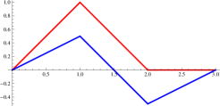
Figure 1. Example 1: $U$ in red, $u_{\infty,D}$ in blue.

Example 2

Let $f=-\chi_{(0,1)},$ $\Omega=(0,3).$ Now we consider the obstacle $\varphi=-\frac{1}{2}.$ The solution to the variational inequality (1.1) is

$$u_{p}=\begin{cases}\frac{((\frac{\beta+1}{2})^{\frac{1}{\beta+1}}-x)^{\beta+1}-\frac{\beta+1}{2}}{\beta+1}&\qquad 0\leq x\leq(\frac{\beta+1}{2})^{\frac{1}{\beta+1}}\\ -\frac{1}{2}&\qquad(\frac{\beta+1}{2})^{\frac{1}{\beta+1}}<x\leq c_{p}\\ -\frac{1}{2}+\frac{(x-c_{p})^{\beta+1}}{\beta+1}&\qquad c_{p}<x\leq 1\\ (1-c_{p})^{\beta}(x-3)&\qquad 1<x\leq 3\end{cases}$$ (5.6)

where

$$\beta=\frac{1}{p-1}$$

and

$$\frac{1}{2}=2(1-c_{p})^{\beta}+\frac{(1-c_{p})}{\beta+1}^{\beta+1}.$$ (5.7)

As $p\to\infty$, from (5.7), we obtain that $c_{p}\to 1^{-},$ $(1-c_{p})^{\beta}\to\frac{1}{4}$ and the limit of functions $u_{p}$ is

$$U=\begin{cases}-x&\qquad 0\leq x\leq\frac{1}{2}\\ -\frac{1}{2}&\qquad\frac{1}{2}<x\leq 1\\ \frac{1}{4}(x-3)&\qquad 1<x\leq 3.\end{cases}$$ (5.8)

While the limit of the solutions to Problems (2.1) with homogeneous Dirichlet conditions is

$$u_{\infty,D}=\begin{cases}-x\qquad 0\leq x\leq 1\\ \frac{x-3}{2}\qquad 1<x\leq 3.\end{cases}$$ (5.9)

We note that, in this example, all assumptions of Theorems 3.1 and 4.6 are satisfied, in particular $\Gamma_{p}=[(\frac{\beta+1}{2})^{\frac{1}{\beta+1}},c_{p}],$    $c_{p}\to 1^{-}$ and $\lim\Gamma_{p}=[\frac{1}{2},1]=\Gamma_{\infty}.$

Remark 5.3.

We note a peculiarity of the limit of solutions to obstacle problems (1.1).

In Example 1 the functions $u_{p}$ in (5.3) converge to $U$ in (5.5) while the functions $-\bigtriangleup_{p}u_{p}$ converge to $f^{*}=\chi_{(1,\frac{3}{2})}-\chi_{(\frac{3}{2},2)}.$ Hence the limit $U^{*}$ of the solutions $u_{p}^{*}$ of the Dirichlet problem (2.1) with datum $f^{*}$ and homogeneous Dirichlet conditions, coincides with the function $u_{\infty,D}$ in (5.2) that does not belong to the convex $\mathcal{K}^{\infty}.$

In Example 2 the functions $u_{p}$ in (5.6) converge to $U$ in (5.8) while the functions $-\bigtriangleup_{p}u_{p}$ converge to $f^{*}=-\chi_{(0,\frac{1}{2})}.$ Hence the limit $U^{*}$ of the solutions $u_{p}^{*}$ of the Dirichlet problem (2.1) with datum $f^{*}$ and homogeneous Dirichlet conditions, is

$$U^{*}=\begin{cases}-x&\qquad 0<x\leq\frac{1}{2}\\ -\frac{1}{2}+\frac{1}{5}(x-\frac{1}{2})&\qquad\frac{1}{2}<x\leq 3\end{cases}$$

that belongs to the convex $\mathcal{K}^{\infty},$ but it is not a mazimizer of (1.6).

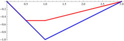
Figure 2. Example 2: $U$ in red, $u_{\infty,D}$ in blue.

Example 3

Let $f=\chi_{(0,1)}-\chi_{(2,3)},$    $\Omega=(0,3).$

The limit of the solutions to (2.1) with homogeneous Dirichlet conditions, is

$$u_{\infty,D}=\begin{cases}x&\qquad 0\leq x\leq\frac{3}{4}\\ \frac{6}{4}-x&\qquad\frac{3}{4}<x\leq\frac{9}{4}\\ x-3&\qquad\frac{9}{4}<x\leq 3.\end{cases}$$ (5.10)

Now we consider the obstacle $\varphi=0.$ The solutions to the variational inequality (1.1) is

$$u_{p}=\begin{cases}\frac{c_{p}^{\beta+1}-(c_{p}-x)^{\beta+1}}{{\beta+1}}&\qquad 0\leq x\leq c_{p}\\ \frac{c_{p}^{\beta+1}-(x-c_{p})^{\beta+1}}{{\beta+1}}&\qquad c_{p}<x\leq 1\\ (1-x)(1-c_{p})^{\beta}+\frac{c_{p}^{\beta+1}-(1-c_{p})^{\beta+1}}{{\beta+1}}&\qquad 1<x\leq 2\\ \frac{(3-x-c_{p})}{\beta+1}^{\beta+1}&\qquad 2<x\leq 3-c_{p}\\ 0&\qquad 3-c_{p}<x\leq 3\end{cases}$$ (5.11)

where

$$\beta=\frac{1}{p-1}$$

and

$$-(1-c_{p})^{\beta}+\frac{c_{p}^{\beta+1}}{\beta+1}=2\frac{(1-c_{p})}{\beta+1}^{\beta+1}.$$ (5.12)

As as $p\to\infty,$ from (5.12), we obtain that $c_{p}\to 1,$ $(1-c_{p})^{\beta}\to 1$ and the limit of functions $u_{p}$ is

$$U=\begin{cases}x&\qquad 0\leq x\leq 1\\ 2-x&\qquad 1<x\leq 2\\ 0&<2\leq x\leq 3.\end{cases}$$ (5.13)

The solution (5.13) of Problem (1.6) differs from the solution (5.10) of problem (2.3) with homogenous Dirichlet data, moreover $U\neq u_{\infty,D}\vee 0.$

Remark 5.4.

In Example 3, the datum $f$ changes sign in $\Omega$ and it is equal to $0$ in a set of positive measure. All assumptions of Theorem 3.1 are satisfied, in particular $\Gamma_{p}=[3-c_{p},3],$    $c_{p}\to 1^{-}$ and $\lim\Gamma_{p}=[2,3]=\Gamma_{\infty}.$ We note that also assumptions (4.13) and (4.14) are satisfied. As we cannot use comparison principles (see [17]), then we do not know whether the viscosity solution to problem (1.6) is unique: in any case Theorems 3.1 and 4.2 select the variational solution $U,$ limit of the functions $u_{p}.$

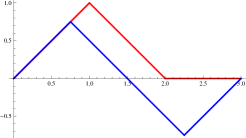
Figure 3. Example 3: $U$ in red, $u_{\infty,D}$ in blue.

Example 4

Let $f=\chi_{(-2,-\frac{3}{2})\bigcup(\frac{3}{2},2)},$ $\Omega=(-2,2).$

Now we consider the obstacle $\varphi=1-x^{2}.$ The solutions to the variational inequality (1.1) is

$$u_{p}=\begin{cases}1-x^{2}&\qquad|x|\leq c_{p}\\ -2c_{p}|x|+1+c_{p}^{2}&\qquad c_{p}<|x|\leq\frac{3}{2}\\ \frac{-(|x|-\frac{3}{2}+(2c_{p})^{p-1})^{\beta+1}+(2-\frac{3}{2}+(2c_{p})^{p-1})^{\beta+1}}{\beta+1}&\qquad\frac{3}{2}<|x|\leq 2\end{cases}$$ (5.14)

where

$$\beta=\frac{1}{p-1}$$

and

$$c^{2}_{p}+1-3c_{p}=\frac{(\frac{1}{2}+(2c_{p})^{p-1})^{\beta+1}-(2c_{p})^{p}}{\beta+1}.$$ (5.15)

As $p\to\infty,$ from (5.15), we obtain that $c_{p}\to\frac{3-\sqrt{7}}{2}$ and the limit of functions $u_{p}$ is

$$U=\begin{cases}1-x^{2}&\qquad|x|\leq\frac{3-\sqrt{7}}{2}\\ -(3-\sqrt{7})|x|+1+\frac{8-3\sqrt{7}}{2}&\qquad\frac{3-\sqrt{7}}{2}<|x|\leq\frac{3}{2}\\ 2-|x|&\qquad\frac{3}{2}<|x|\leq 2.\end{cases}$$ (5.16)

The solution $u_{\infty,D}$ of Problem (2.3) with homogenous Dirichlet data is

$$u_{\infty,D}=\begin{cases}2-|x|&\qquad\frac{3}{2}<|x|\leq 2\\ \frac{1}{2}&\qquad|x|\leq\frac{3}{2}.\end{cases}$$ (5.17)

Remark 5.5.

In this example all assumptions of Theorem 4.3 are satisfied and the function $U$ in (5.16) is a solution to Problem (1.6) and differs from the function $u_{\infty,D}$ in (5.17) that is a solution to Problem (2.3) (with homogenous Dirichlet conditions), moreover $U\neq u_{\infty,D}\vee\varphi.$ Hence Example 4 shows that assumptions of Theorem 4.3 do not imply that the limit of the solutions to Problems (4.21) solves also Problem (1.6): in particular, Theorem 4.3 is not a easy consequence of Theorem 2.4 in [13].

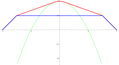
Figure 4. Example 4: $U$ in red, $u_{\infty,D}$ in blue, obstacle in green.

Example 5

Let $f=-\chi_{(-\frac{1}{3},\frac{1}{3})},$ $\Omega=(-1,1).$ Now we consider the obstacle $\varphi=\frac{3}{4}(x^{2}-1).$ The solution to the variational inequality is

$$u_{p}=\begin{cases}\frac{3}{4}(x^{2}-1)&\qquad|x|\leq c_{p}\\ \frac{(|x|+(\frac{3}{2}c_{p})^{p-1}-c_{p})^{\beta+1}-(\frac{1}{3}+(\frac{3}{2}c_{p})^{p-1}-c_{p})^{\beta}(1+(\frac{3}{2}c_{p})^{p-1}-c_{p}+\frac{2\beta}{3})}{\beta+1}&\qquad c_{p}<|x|\leq\frac{1}{3}\\ (\frac{1}{3}+(\frac{3}{2}c_{p})^{p-1}-c_{p})^{\beta}(|x|-1)&\qquad\frac{1}{3}<|x|\leq 1\end{cases}$$ (5.18)

where

$$\beta=\frac{1}{p-1}$$

and

$$\frac{3}{4}(c^{2}_{p}-1)=\frac{(\frac{3}{2}c_{p})^{\frac{\beta+1}{\beta}}-(\frac{1}{3}+(\frac{3}{2}c_{p})^{p-1}-c_{p})^{\beta}(1+(\frac{3}{2}c_{p})^{p-1}-c_{p}+\frac{2\beta}{3})}{\beta+1}.$$ (5.19)

As $p\to\infty,$ from (5.19), we obtain that $c_{p}\to\frac{1}{3},$ $(\frac{1}{3}+(\frac{3}{2}c_{p})^{p-1}-c_{p})^{\beta}\to 1,$ $\Gamma_{p}=[-c_{p},c_{p}],$ $\lim\Gamma_{p}=[-\frac{1}{3},\frac{1}{3}]$ and the limit of functions $u_{p}$ is

$$U=\begin{cases}\frac{3}{4}(x^{2}-1)&\qquad|x|\leq\frac{1}{3}\\ |x|-1&\qquad\frac{1}{3}<|x|\leq 1.\end{cases}$$ (5.20)

In this example, the solution $U$ in (5.20) of Problem (1.6) differs from the function $u_{\infty,D}=-d(x)$ solution to Problem (2.3) with homogenous Dirichlet data.

Remark 5.6.

In Example 5 the assumptions of Theorem 3.1 are satisfied, nevertheless the limit of the solutions to Problems (4.21) does not solve Problem (1.6). In particular Theorem 3.1 is not a easy consequence of Theorem 2.1 in [13].

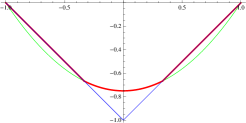
Figure 5. Example 5: $U$ in red, $u_{\infty,D}$ in blue, obstacle in green.

Example 6

Let $\Omega=\{x\in\mathbb{R}^{n}:|x|<2\},\,\,$ $\varphi=1-x^{2}$ and $f=0$ (see example in the Appendix of [19]).

Problem (1.6) does not have a unique solution; in fact both the following functions $U$ and $v^{*}$ are solutions:

$$U=\begin{cases}1-x^{2}&\qquad|x|\leq h\\ -2h|x|+4h&\qquad h<|x|\leq 2\end{cases}$$ (5.21)

where $h=2-\sqrt{3}$ and

$$v^{*}=\begin{cases}1-x^{2}&\qquad|x|\leq\frac{1}{2}\\ -|x|+\frac{5}{4}&\qquad\frac{1}{2}\leq|x|\leq\frac{5}{4}\\ 0&\quad\quad\frac{5}{4}\ <|x|\leq 2.\end{cases}$$ (5.22)

For $p>n$ and $\alpha=\frac{n-1}{p-1}$, we have that the solution to (1.1) is

$$u_{p}=\begin{cases}1-x^{2}\qquad|x|\leq c_{p}\\ \frac{-2c_{p}^{1+\alpha}}{1-\alpha}(|x|^{1-\alpha}-2^{1-\alpha})\qquad c_{p}<|x|\leq 2\end{cases}$$ (5.23)

where

$$(1+\alpha)c_{p}^{2}-2^{2-\alpha}c_{p}^{1+\alpha}+1-\alpha=0.$$ (5.24)

As $p\to\infty,$ from (5.24), we obtain that $c_{p}\to h$ and $\lim\Gamma_{p}=\lim[-c_{p},c_{p}]=[-h,h]=\Gamma_{\infty}.$ The function $U,$ that (according Remark 4.1 of Theorem 4.1) is limit of $u_{p},$ coincides on the annulus $B_{h,2}$ with the AMLE of $g$ ,

$$g=\begin{cases}1-h^{2}&\qquad x\in\partial B_{h}\\ 0&\qquad x\in\partial B_{2}\end{cases}$$ (5.25)

while the function $v^{*}$ is a solution of Problem (1.6), but it is not the AMLE of g.

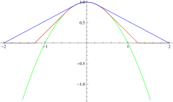
Figure 6. Example 6: $U$ in red, $v^{*}$ in blue, obstacle in green.

Example 7

Let $\Omega=\{x\in\mathbb{R}^{n}:|x|<2\},\,\,$ $\varphi=1-x^{2}$ and $f=-1.$

The function $U,$ limit of $u_{p}$ coincides with the unique viscosity solution to Problem (1.6), $u_{\infty}$ (see Theorem 4.4). More precisely

$$u_{p}=\begin{cases}1-x^{2}&\qquad|x|\leq h_{p}\\ \frac{(-|x|+c_{p})}{\beta+1}^{\beta+1}-\frac{(-c_{p}+2)}{\beta+1}^{\beta+1}&\qquad h_{p}<|x|\leq c_{p}\\ \frac{(|x|-c_{p})}{\beta+1}^{\beta+1}-\frac{(-c_{p}+2)}{\beta+1}^{\beta+1}&\qquad c_{p}\leq|x|\leq 2\\ \\ \end{cases}$$ (5.26)

where

$$\beta=\frac{1}{p-1},\,\,\,(-h_{p}+c_{p})^{\beta}=2h_{p},\,\,(-h_{p}+c_{p})^{\beta+1}-(2-c_{p})^{\beta+1}=(\beta+1)(1-h^{2}_{p}).$$

Then $h_{p}\to\frac{1}{2},\,\,\,c_{p}\to\frac{13}{8}$ and the limit function is

$$U=\begin{cases}1-x^{2}\qquad|x|\leq\frac{1}{2}\\ \frac{5}{4}-|x|\qquad\frac{1}{2}<|x|\leq\frac{13}{8}\\ |x|-2\qquad\frac{13}{8}<|x|\leq 2,\end{cases}$$ (5.27)

while the function $u_{\infty,D}$ coincides with the opposite of the distance from the boundary, $u_{\infty,D}=-d(x)=2-|x|.$

GRANTS The authors are members of GNAMPA (INdAM) and are partially supported by Grant Ateneo “Sapienza” 2017.

References

- [1] J. Andersson, E. Lindgren, H. Shahgholian, Optimal regularity for the obstacle problem for the p-Laplacian, J. Differential Equations 259 (2015), no. 6, 2167–2179.
- [2] G. Aronsson, M. G. Crandall, P. Juutinen, A tour of the theory of absolutely minimizing functions, Bull. Amer. Math. Soc. (N.S.) 41 (2004), no. 4, 439–505.
- [3] T. Bhattacharya, E. DiBenedetto, J. Manfredi, Limits as of and related extremal problems, Some topics in nonlinear PDEs (Turin, 1989), Rend. Sem. Mat. Univ. Politec. Torino 1989, Special Issue, 15–68 (1991).
- [4] P. Blanc, J. V. da Silva, J. D. Rossi, A limiting free boundary problem with gradient constraint and Tug-of-War games, Annali di Matematica Pura ed Applicata 198 (2019), no. 4, 1441–1469.
- [5] G. Bouchitté, G. Buttazzo, L. De Pascale, A p-Laplacian approximation for some mass optimization problems, J. Optim. Theory Appl. 118 (2003), no. 1, 1–25.
- [6] F. Camilli, R. Capitanelli, M. A. Vivaldi, Absolutely Minimizing Lipschitz Extensions and Infinity Harmonic Functions on the Sierpinski gasket, Nonlinear Anal. 163 (2017), 71–85.
- [7] R. Capitanelli, S. Fragapane, Asymptotics for quasilinear obstacle problems in bad domains, Discrete Contin. Dyn. Syst. Ser. S 12 (2019), no. 1, 43–56.
- [8] R. Capitanelli, S. Fragapane, M. A. Vivaldi, Regularity results for p-Laplacians in pre-fractal domains, Adv. Nonlinear Analysis 8 (2019), no. 1, 1043–1056.
- [9] R. Capitanelli, M. A. Vivaldi, FEM for quasilinear obstacle problems in bad domains, ESAIM Math. Model. Numer. Anal. 51 (2017), no. 6, 2465–2485
- [10] L. C. Evans, W. Gangbo, Differential equations methods for the Monge-Kantorovich mass transfer problem, Mem. Amer. Math. Soc. 137 no. 653 (1999).
- [11] M. Feldman, R.J. McCann, Uniqueness and transport density in Monge’s mass transportation problem, Calc. Var. Partial Differential Equations 15 (2002), no. 1, 81–113.
- [12] A. Figalli, B. Krummel, X. Ros-Oton, On the regularity of the free boundary in the p-Laplacian obstacle problem, J. Differential Equations 263 (2017), no. 3, 1931–1945.
- [13] H. Ishii, P. Loreti, Limits of solutions to p-Laplace equations as p goes to infinity and related variational problems, SIAM J. Math. Anal. 37 (2005), no. 2, 411–437.
- [14] K. Kuratowski, Topology. Volumes I and II. New edition, revised and augmented. New York: Academic Press.
- [15] R. Jensen, Uniqueness of Lipschitz extensions: minimizing the sup norm of the gradient, Arch. Rational Mech. Anal. 123 (1993), no. 1, 51–74.
- [16] P. Juutinen, M. Parviainen, J. D. Rossi, Discontinuous gradient constraints and the infinity Laplacian. Int. Math. Res. Not. IMRN 2016, no. 8, 2451–2492.
- [17] G. Lu, P. Wang, Inhomogeneous infinity Laplace equation, Adv. Math. 217 (2008), 1838–1868.
- [18] J. M. Mazón, J. D. Rossi, J. Toledo, Mass transport problems for the Euclidean distance obtained as limits of p-Laplacian type problems with obstacles, J. Differential Equations 256 (2014), 3208–3244.
- [19] J. D Rossi, E. V. Teixeira, J. M. Urbano, Optimal regularity at the free boundary for the infinity obstacle problem, Interfaces Free Bound. 17 (2015), no. 3, 381–398.
- [20] G. M. Troianiello, Elliptic Differential Equations and Obstacle Problems, Springer, 1987.
- [21] C. Villani, Optimal transport. Old and new, Grundlehren der Mathematischen Wissenschaften [Fundamental Principles of Mathematical Sciences], 338. Springer-Verlag, Berlin, 2009.