Precision of the ENDGame: Mixed-precision arithmetic in the iterative solver of the Unified Model.

Abstract

The Met Office’s weather and climate simulation code the Unified Model is used for both operational Numerical Weather Prediction and Climate modelling. The computational performance of the model running on parallel supercomputers is a key consideration. A Krylov sub-space solver is employed to solve the equations of the dynamical core of the model, known as ENDGame. These describe the evolution of the Earth’s atmosphere. Typically, 64-bit precision is used throughout weather and climate applications. This work presents a mixed-precision implementation of the solver, the beneficial effect on run-time and the impact on solver convergence. The complex interplay of errors arising from accumulated round-off in floating-point arithmetic and other numerical effects is discussed. A careful analysis is required, however, the mixed-precision solver is now employed in the operational forecast to satisfy run-time constraints without compromising the accuracy of the solution.

1 Introduction

Numerical simulations of the fluid dynamics of the Earth’s atmosphere, which are central to all weather and climate models, require solutions to a non-linear system of partial differential equations (PDEs). These PDEs are recast into a discrete system of algebraic equations on a grid covering the Earth. For each grid cell, the fluid dynamic properties of the atmosphere, the velocity, temperature, pressure and density of the air, are then to be determined.

When deriving these algebraic equations, which arise from the continuous form of the compressible Euler equations, there is a choice of whether to integrate forward in time explicitly (a direct calculation) or (semi-)implicitly. The latter involves a global matrix inversion of some form. For Numerical Weather Prediction (NWP) simulations, particularly those discretised onto a longitude-latitude (lon-lat) grid, the nature of the grid means that it is generally not feasible to use an explicit scheme as it would severely restrict the length of the time step employed in the simulation. A typical operational global NWP simulation is required to simulate seven to fourteen days within one-to-two hours of wall-clock time and the number of small time steps of the explicit scheme would either be prohibitively expensive, or severely limit the physical complexity or spatial resolution of an affordable simulation.

Semi-implicit schemes treat the short-timescale accoutic-gravity modes implicitly and allow a stable integration of the flow around the polar singularity and in regions with strong horizontal flows. To an extent, these schemes also allow more flexibility in the formulation of the algebraic system and in particular the form of the global matrix inversion. In line with incompressible and low Mach number flows, a pressure correction equation is derived which takes the form

$$A\cdot{\mathbf{x}}={\mathbf{b}},$$ (1)

where $A$ is a large, sparse (banded) matrix of order $n$, ${\mathbf{x}}$ is the pressure correction / tendency and ${\mathbf{b}}$ contains the explicit forcing terms. This can be solved using a combination of Krylov sub-space iterative solvers, pre-conditioners and parallel computers to satisfy wall-clock time constraints such as those described above.

The current operational configuration of the Met Office Unified Model (UM) [1] solves the dynamical system described above using the “ENDGame” dynamical core [2]. The operational deterministic global forecast is discretised onto an N1280 lon-lat grid with $2560\times 1920$ grid points, giving it a horizontal resolution of approximately 10 km at mid-latitudes. With 70 discrete vertical levels, the number of degrees of freedom $n$ for the pressure correction system is large at approximately 350 million; the full algebraic system is six times larger. For such a large system, a parallel supercomputer is required. However, even on state-of-the-art parallel computers such as the Met Office’s Cray XC40 machine, both algorithmic and code optimisations are necessary to scale to a large degree of parallelism and to execute the program as quickly as possible.

One potential optimisation is to consider the numerical precision to which variables in the code are computed and stored, as reducing the precision can provide performance advantages. In common with many scientific numerical applications, weather and climate codes are memory bound. Using smaller data types reduces data movement between memory and CPU and reduces remote communication between processors, such that this is faster and uses less energy. Moreover, caches can be utilised more effectively. For weather and climate models, however, knowledge of accuracy and uncertainty are important. There are many processes that affect the evolution of the system that are either not resolved at the cut-off scale imposed by the discretisation or are not represented by the dynamical core. These processes are represented by physical parametrizations, which often include many branches in the code. For example, the presence or not of liquid water in a grid cell will determine whether latent heat can be released through the freezing of that water; this in turn will affect the temperature of the atmosphere and so influence the evolution of the dynamics. An aversion to the possibility of compromising the accuracy of a simulation through either accumulated round-off errors, or round-off errors triggering different branches with parametrizations, has led to the “safety first” approach of using high precision arithmetic throughout, and the assumption that this is both necessary and more accurate. In common with many scientific applications, therefore, 64-bit floating point arithmetic – often referred to as double precision – is used by default and has become the accepted standard.

Recent work [3, 4, 5, 6] and [7] has explored the potential benefits of moving away from the use of 64-bit arithmetic throughout an atmospheric model. These papers examine a variety of approaches to reducing precision, from low precision emulators, Field Programmable Gate Arrays (FPGAs), toy models, right through to running a full atmospheric model in 32-bit precision (i.e. single precision) to examine the effect of precision on forecast accuracy. Whilst it is true that 64-bit precision may be desirable, if not required, for some portions of the simulation, many schemes within a model will have either physical or parametric uncertainty, or will be designed to reach an approximate solution, with accuracy far removed from the numerical precision of the variables within the scheme. One such example is the numerical solution of Equation (1). The solution for the pressure correction $\mathbf{x}$ is obtained through an iterative solver, in which each variable is typically defined to double precision, but in which the calculation is halted when the normalised error has reduced by only a small number of orders of magnitude. Whilst the solver is only a small proportion of the total code base when measured by the number of lines of code, at the resolutions and node counts described for operational global NWP above, these routines constitute approximately one quarter of the run time of the full simulation. In this work, a mixed-precision solver is defined, in which the pressure field itself is held in double precision throughout, but the majority of calculations, and hence the majority of memory transfers, are performed in single precision. In section 2 the ENDGame dynamical core, the Helmholtz equation to be solved for the pressure correction and the pre-conditioner used for this are described. In section 3 the mixed-precision solver is described, whilst in section 4 the effect this has on convergence to the solution as well as the computational speed up obtained is discussed. Finally, conclusions are drawn in section 5.

2 The ENDGame Dynamical core

Symbolically, the linear system of equations to be solved is of the form

$$\left(\begin{array}[]{cccccc}I&0&0&0&0&G_{u}\\ 0&I&0&0&0&G_{v}\\ 0&0&I&B_{i}&0&G_{w}\\ 0&0&B_{ii}&I&0&0\\ D_{x}&D_{y}&D_{z}&0&I&0\\ 0&0&0&E_{\theta}&I&E_{\pi}\end{array}\right)\left(\begin{array}[]{c}u\\ v\\ w\\ \theta\\ \rho\\ \Pi\end{array}\right)=\left(\begin{array}[]{c}R_{u}\\ R_{v}\\ R_{w}\\ R_{\theta}\\ R_{\rho}\\ R_{\Pi}\end{array}\right)$$ (2)

where $I$ represents identity matrices, $G_{u,v,w}$ are discrete pressure gradient terms, $D_{x,y,z}$ are components of the divergence operator, $B_{i}$ and $B_{ii}$ are the coupling between the potential temperature and the vertical component of velocity due to gravity and $E_{\theta,\rho}$ arise from linearisation of the equation of state. The solution of this system corresponds to the fluid velocity components $(u,v,w)$ and the tendencies (change between time steps) of the thermodynamic variables $\rho$ (density), $\Pi$ (Exner pressure) and $\theta$ (potential temperature). Note that within the ENDGame formulation, due to non-linearities and the change to a terrain following coordinate system, the right hand side terms involve contributions from the previous iterates of the current time step. Typically this linear system is solved four times per time step and so the solution method needs to be efficient.

This matrix is of the general form

$$\left(\begin{array}[]{cc}P&Q\\ R&S\end{array}\right)\left(\begin{array}[]{c}{\mathbf{y}}\\ {\mathbf{x}}\end{array}\right)=\left(\begin{array}[]{c}{\mathbf{s}}\\ {\mathbf{t}}\end{array}\right)$$ (3)

which can be solved using the Schur compliment as

$${\mathbf{y}}=P^{-1}({\mathbf{s}}-Q{\mathbf{x}});\hskip 7.22743ptA{\mathbf{x}}=(S-RP^{-1}Q){\mathbf{x}}={\mathbf{t}}-RP^{-1}{\mathbf{s}}={\mathbf{b}}.$$ (4)

The matrix $A$ has a $7$-band structure similar to what would be expected from discretising the Laplacian operator, which, would be its exact equivalent in the Boussinesq incompressible limit. In the full system, however, it differs in some key aspects. Firstly, the matrix is non-symmetric and it is not constant coefficient; i.e., the matrix rows are all different due to the spherical nature of the Earth and variations in temperature and orography (the height of the lower boundary). Secondly, as may be anticipated from the previous sentence, the matrix is time varying and so needs to be recomputed at every time step. This precludes the ability to pre-factorise the matrix off-line. Finally, because the vertical length scales are much shorter than the horizontal and gravitational effects are far larger than the vertical accelerations, some care is needed in order to solve this matrix. In particular, it is necessary to ensure that the large scale hydrostatic balance is maintained during the iterations. It should be noted that, since this equation arises from a non-linear algebraic system, there are terms involving ${\mathbf{x}}$ which are lagged and so appear as forcing in the right-hand-side ${\mathbf{b}}$ (see [2] for further details).

The system in equation (4) is solved using a Krylov subspace solver based on a “post-conditioned” variant of the BiCGstab algorithm [8] and so is replaced by

$$D^{-1}_{g}ACC^{-1}{\mathbf{x}}=D^{-1}_{g}{\mathbf{b}}\hskip 7.22743pt\equiv\hskip 7.22743pt\hat{A}CC^{-1}{\mathbf{x}}=\hat{\mathbf{b}},$$ (5)

where $D_{g}$ is the diagonal of $A$ and $C$ is the pre-conditioner. BiCGstab is used rather than the Conjugate Gradient algorithm [9] due to the lack of symmetry in the derived matrix $A$. The application of the diagonal is performed outside the solver and reduces the need to access this term during the application of $A{\mathbf{x}}$ within the Krylov method. The application of $C$ is performed through a few (typically three) iterations of a second stationary method derived from the Successive-Over-Relaxation method (SOR), but with a decomposition that better reflects the nature of the atmospheric problem. This is achieved by writing

$$\hat{A}=L+T+U,$$ (6)

where $T$ is a tridiagonal matrix arising from the vertical discretisation, $L$ is a lower triangular matrix and $U$ is an upper triangular matrix. Following the standard derivation of SOR, the fixed point method is obtained.

$$(T+\omega L){\mathbf{x}}_{n}=(1-\omega)T{\mathbf{x}}_{n-1}+\omega(r-U\mathbf{x}_{n-1}),$$ (7)

where $\omega=1.5$ is the over-relaxation parameter and the only difference from the standard method is the appearance of the tridiagonal matrix $T$ in place of the diagonal. Note that the lower/upper-factorisation of the matrix $T$ can be pre-computed (at each horizontal grid point) to aid the inversion process. Furthermore, there is no parallel decomposition in the vertical, which simplifies the process of applying $T^{-1}$ considerably.

3 The Mixed-Precision Solver

The accuracy of the solution reached by the BiCGstab solver is determined by the halting criterion

$$\|{\bf r}_{i}\|=\|{\bf b}-A\cdot{\bf x}_{i}\|,$$ (8)

where ${\bf x}_{i}$ is the solution after $i$ iterations and ${\bf r}_{i}$ is known as the residual vector. If the norm of ${\bf r}_{i}$ is small, then ${\bf x}_{i}$ is likely to be close to the solution ${\bf x}$. The halting criterion for this algorithm is to break out of the iteration loop when the residual (either absolute or relative) has fallen below some threshold. The relative norm of the residual (R), is defined as

$$\mathrm{R}=\frac{\|\mathbf{r}_{i}\|}{\|\mathbf{b}\|}$$ (9)

and then the halting criterion is defined as when ${\mathrm{R}}<{\mathrm{R}}_{c}$, where ${\mathrm{R}}_{c}$ is known as the critical residual or the “solver tolerance”. The optimum value of ${\mathrm{R}}_{c}$ is determined by a compromise between the desired accuracy of the solution and its computational cost.

In floating point arithmetic, the Unit of Least Precision (ULP) is defined in [10] as follows. The ULP in $x$ is the distance between the closest two straddling IEEE floating point numbers $a$ and $b$, i.e. those with $a\leq x\leq b$. For numbers ${\mathcal{O}}(1)$ this is ${\mathcal{O}}(10^{-7})$ for 32-bit numbers and ${\mathcal{O}}(10^{-15})$ for 64-bit. If the stopping criterion

$${\mathrm{R}}_{c}\gg\epsilon_{32},$$ (10)

where $\epsilon_{32}$ is the ULP or machine precision for 32-bit floating point numbers, then 32-bit floating point numbers can satisfy the desired accuracy. Iterative methods in general are discussed in [11]. In chapter 4, section 2, on the stopping criterion, the authors discuss accuracy and error. They show that the stopping criterion should not be set such that ${\mathrm{R}}_{c}<\epsilon$, Where $\epsilon$ is the precision in the calculation. used Conversely, decreasing $\epsilon$ from, for instance, $10^{-7}$ for 32-bit precision to $10^{-15}$ for 64-bit precision has no effect on the accuracy of the solution if ${\mathrm{R}}\gg\epsilon_{\rm 32}$.

In the case of the semi-implicit time stepping scheme, the solution to the linear system is part of the solution procedure [2] to a larger, non-linear system and the accuracy of the solve is dictated by the need for stability of the time stepping scheme. Moreover, it is only an indirect measure of the error. It is worth noting that since the finite difference approximations to the pressure gradient are at best second order, there is a limit to the effect of tightening the solver tolerance on the pressure. i.e. once the error in the solver is sufficiently small, the discretisation error becomes dominant.

In its first implementation, all operational systems using ENDGame used a tolerance of ${\mathrm{R}}_{c}=10^{-3}$, which easily satisfies the condition laid out in equation (10). These calculations can be done in 32-bit without loss of accuracy compared to a calculation done in 64-bit, which offers a significant optimisation opportunity, especially as the solver and the pre-conditioner are memory bound. A 32-bit version of the code has in effect, twice the cache memory available compared to a 64-bit version. This motivated the use of the mixed-precision solver, which contributed to the optimisations that made the implementation computationally affordable.

In principle, the whole BiCGStab algorithm could be written in 32-bit. However, the rest of the model remains 64-bit. The two components have been combined and it is natural to encapsulate the solver algorithm as a subroutine. It is not possible in Fortran to coerce a 64-bit real to a 32-bit real as an argument to a subroutine, modify its value and promote it back safely to a 64-bit real when the subroutine exits. So, rather than pay the cost of a whole domain memory copy from 64- to 32-bit when entering the routine and again on exit, the pressure field is kept as a 64-bit data-type and so mixed precision arithmetic is required. Most of the operations, including communications, can be performed in single precision and the Fortran run-time can coerce or promote the remaining operations automatically.

Following the initial implementation of ENDGame, numerical noise was observed in the horizontal wind field near the pole, which could be alleviated by tightening the solver tolerance [12], although it remains unclear whether the noise was a direct feature of insufficient convergence in the vicinity of the pole, or was created by some other numerical issue and removed/reduced through additional iterations of the pressure solver. The latest operational global configuration uses a tolerance of ${\mathrm{R}}_{c}=10^{-4}$, which although an order of magnitude tighter than originally used, still satisfies the inequality in (10).

4 Numerical and computational performance

To test the convergence of the solver, a serial toy-model of the ENDGame solver was constructed. The toy-model is simply the BiCGstab solver and pre-conditioner with $\mathbf{x}$ initialised to a representative pressure field, the Helmholtz matrix with the correct structure for ENDGame and representative right-hand side $\mathbf{b}$ values. No halting criterion is used, but instead the solver is run to very high levels of convergence, to study the convergence behaviour of R. Shown in figure (1) is the value of R for a 32-bit and 64-bit solver as a function of time step.

Figure 1: The relative norm of residual, R defined in equation (9) versus iteration number. The blue line, labelled “DP” shows data from the 64-bit solver, the red line, labelled “SP” is the 32-bit solver.

Both 32- and 64-bit solvers show the non-monotonic convergence typical of the BiCGStab algorithm. For the first few iterations, convergence is sufficiently similar to be indistinguishable. Around ${\mathrm{R}}=10^{-3}$, the 32-bit version takes one extra iteration to reach the same value of R. This “iteration gap” grows as the residual falls. At tighter convergence, the 32-bit version takes twice as many iterations to reach ${\mathrm{R}}=10^{-7}$ as the 64-bit version. This may well be due to the loss of orthogonality in the Krylov sub-space vectors. In the BiCGstab algorithm, these vectors are updated each iteration, they are not re-computed. Accumulated round-off errors set in earlier for the lower precision versions. The estimate of these vectors becomes worse with increasing iteration number resulting in a loss of efficiency. This can be recovered by restarting the algorithm; this comes at the cost of re-computing the vectors, but this restores the orthogonality of the Krylov sub-space. Intriguingly, the break-even point for the 32-bit solver is ${\mathrm{R}}\approx 10^{-7}$, i.e. the limit of 32-bit precision. Here, the 32-bit version takes twice as many iterations as the 64-bit version but each iteration is twice as fast.

The decision to implement the mixed-precision solver in the full model was based on tests using comprehensive weather and climate model simulations. These included high resolution 5-day NWP forecast runs and further testing in an operational-like research NWP system. Results with the mixed-precision and double precision solvers showed no noticeable scientific differences and hence the mixed-precision solver was accepted. To study the behaviour of the solver in more detail in an operational-like forecast, a set of N1280 global model simulations were run for a series of 11 dates each separated by one week, each on 96 nodes of the Met Office Cray XC40. Mixed- and double precision solver runs for each date were initialised from 64-bit model states ${\mathbf{x}}$, saved from a previous short forecast. Each XC40 node is dual socket, each with an 18-core Intel Xeon (Broadwell) processor. The model is parallelised with both MPI and OpenMP by domain decomposition across the two dimensional horizontal domain. It was run with six MPI ranks per socket and three OpenMP threads per MPI rank. Again, the convergence was measured using the residual R defined in equation (9). Shown in figure (2) is the value of R versus the iteration number, for the mixed- and double precision version, up to the operational convergence criterion of ${\mathrm{R}}_{c}=10^{-4}$, The data for convergence of the solvers is also shown in table (1).

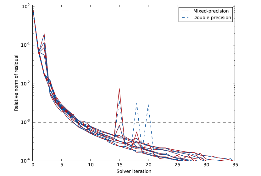
Figure 2: The relative norm of residual, R defined in equation (9) versus iteration number from the first call to the solver in 11 simulation dates each run with the mixed- and double precision solver.

The results presented from each date are from the first call to the solver in the first model time step, so that the prognostic fields on entering the solver are identical between the mixed- and double precision versions, so as to make it simple to compare the behaviour between the two. There are several features in the figure worth remarking on. Firstly, for the first five iterations, the fall in the size of the residual is quite steep, showing quick convergence, although four of the eleven sets of simulations demonstrate the lack of guaranteed monotonicity, even this early on. Secondly, up to and slightly beyond the original operational halting criterion of ${\mathrm{R}}_{c}=10^{-3}$, the values of ${\mathrm{R}}_{\rm MP}$ and ${\mathrm{R}}_{\rm DP}$ are very close, where $MP$ denotes mixed-precison and $DP$ double or 64-bit precsion. After a single iteration, these agree for every date to seven significant figures, i.e. roughly the precision of a 32-bit number. Also, for each date, the residual reaches the halting criterion in an identical number of iterations, and the values of ${\mathrm{R}}_{\rm MP}$ and ${\mathrm{R}}_{\rm DP}$ at that point all agree to at least four significant figures. Between ${\mathrm{R}}=10^{-3}$ and ${\mathrm{R}}=10^{-4}$, the rate of convergence slows down and in a few cases jumps to a value an order of magnitude higher before dropping back down again, although these jumps are present in both the mixed- and double precision solver, and appear not to be related to the precision of the calculations.

The time taken to reach ${\mathrm{R}}\leq 10^{-3}$ and ${\mathrm{R}}\leq 10^{-4}$ is shown in Table 1. The mixed-precision BiCGStab is almost twice as fast per iteration than the 64-bit version, for the reasons outlined in section 1, viz. that the smaller data type halves the data movement both from memory to CPU and remote communication and doubles the number of data items in the memory caches. For example, the local volume for each MPI rank/OpenMP thread is

$$LV=(l_{x}+2h_{x})\times(l_{y}+2h_{y})\times n_{levels}/n_{threads}$$ (11)

where $l$ is local domain size, $h$ the halo size, $x$ the East-West direction, $y$ the North-South directions, $n_{levels}$ is the number of vertical levels and $n_{threads}$ is the the number of OpenMP threads the data are shared between. For a 96 node (3456 core) job, a typical decomposition might be 72 MPI ranks East-West and 16 North-South with 3 OpenMP threads resulting in a local volume of

$$LV=\left(\frac{2560}{72}+2\right)\times\left(\frac{1920}{16}+2\right)\times 70/3=111720$$ (12)

The pre-conditioner routine, called tri_sor, requires ten domain valued arrays for the 7-point stencil and back substitution. Thus the size of the working set, $N$, is

$$N=111720\times 10=1117200$$ (13)

The memory footprint for a working set of this size is 4468800 bytes in 32-bit and 8937600 bytes in 64-bit. The Met Office supercomputer processors are Intel Xeon E5-2695 v4, which has a level 2 (L2) cache of size 4718592 bytes. The working set would fit into L2 cache in 32-bit. Of course, what data are resident in cache is much more complicated than simple size. However, the working set clearly cannot fit into L2 cache in 64-bit. Other levels of cache, main memory bandwidth and remote communication bandwidth will all affect the speed of computation and by using smaller data these can be exploited more effectively.

Table 1: The mean (standard error) iteration count and wall clock time taken in seconds for the mixed- and double-precision solvers to reach the converge to the halting criterion ${\mathrm{R}}_{c}$.

	Mixed-precision		Double precision
R	Iterations	Time (s)	Iterations	Time (s)
$10^{-3}$	$8.4(2)$	$0.346(6)$	$8.4(2)$	$0.592(9)$
$10^{-4}$	$29.3(9)$	$1.18(2)$	$29.3(9)$	$2.06(3)$

To see the effect on the iteration count and convergence of the algorithm for this work, the simulations from figure (2) have been extended to use a tighter halting criterion of ${\mathrm{R}}_{c}=10^{-5}$, which is shown in figure (3).

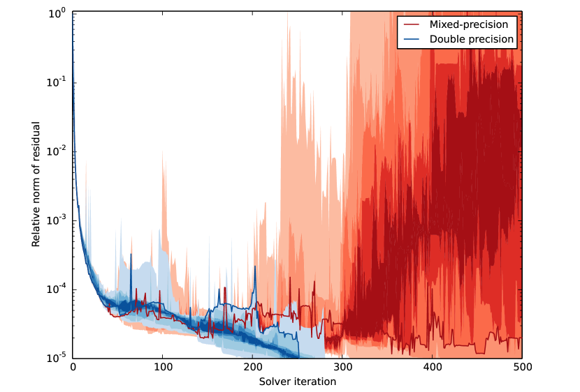
Figure 3: . The relative norm of residual, R defined in equation (9) versus iteration number from the same simulations presented in figure 2, but with the tighter halting criterion of ${\mathrm{R}}_{c}=10^{-}5$. Shading is used to highlight the ranges of ${\mathrm{R}}$ per iteration, with a “typical” single case highlighted in the solid lines.

This shows that when ${\mathrm{R}}<10^{-4}$, the BiCGstab algorithm starts to break down as beyond this point, the value of the residual falls slowly and often jumps to a higher value between iterations. The simulations with the double precision solver take hundreds of iterations to converge to ${\mathrm{R}}\leq 10^{-5}$, and can experience many jumps before this occurs. Below ${\mathrm{R}}\approx 10^{-4}$, however, it is clear that the mixed-precision approach suffers from severe errors and after 500 iterations, only two of the simulations have converged, whilst others have become unstable and the residual has started growing rather than reducing with time.

In operational simulations, occasional problems with convergence have been observed even with ${\mathrm{R}}_{c}=10^{-4}$. In these cases, the scalar weights of the BiCGStab algorithm are close to or equal to zero and dividing by these very small numbers can result in floating-point overflows and the algorithm failing. The scalars are calculated by a global sum, which in the original mixed-precision solver were performed in 32-bit, with the local summation performed first, then an MPI reduction call on a single number. To protect against the scalars summing to zero, however, the global sum only has since been reverted to 64-bit. This has a negligible cost as the MPI reduction is the dominant cost of the procedure and this is latency bound. Reverting the global sums to 64-bit reduces the likelihood of the model failing with overflowing fields, but the problem of slow convergence remains. Slow convergence can be the result of a loss of orthogonality of the Krylov sub-space, although there are multiple reasons for which BiCGStab can break down [13]. To address this and improve the robustness of operational systems, the implementation of BiCGStab was modified to include a mandatory restart if convergence has not been achieved after a fixed number of iterations. The restart threshold is set at a relatively high number of iterations of 150. The results above suggest that this poor convergence could be either due to the general convergence issues seen in both the mixed- and double precision solvers, or due to the additional rounding errors seen in the mixed-precision solver with very small values of $R$.

5 Conclusion

Speed, accuracy and stability of computation are all important criteria for numerical calculations, particularly for an operational NWP system. When carefully controlled, the use of reduced precision can have a big impact on the speed of a calculation without affecting its accuracy or stability. However, as shown in this work, for a complex system that is susceptible to non-convergence of the numerical algorithm employed to solve it, reduced precision can only be safely employed within a certain regime.

There are undoubted benefits to reducing precision, in this case halving the run-time of the solver. However, other numerical instabilities such as the polar noise described in a previous section have forced the model to be run on a regime where the iterative, Krylov solver has problems with slow convergence. This makes the use of reduced precision all the more important as the run-times with a tighter stopping criteria are longer. Naively, it should be possible to run with reduced precision at tighter stopping condition than $10^{-4}$, however, problems with slow convergence and numerical stability indicate that the algorithm used, BiCGStab, is failing, either to converge or doing so far too slowly. This is true for the double-precision version and so it is safe to conclude that these issues are not caused by using reduced precision. However, as the reduced precision version appears to suffer more severe problems, including failing to converge, it is clear that there is a complex interplay between accumulated round-off errors and other errors introduced by the numerical scheme.

These issues, combined with the behaviour shown in figure (3), suggest that there could be some benefit from continuing to investigate the cause of the noise in the horizontal wind field near the pole. This may allow the operational forecasts to revert to the slacker solver tolerance of $R_{c}=1.0\times 10^{-3}$ and hence make the solution less susceptible to problems with convergence, whilst reducing computational cost. These results also make clear that the poor convergence is not directly related to the mixed-precision solver, and would still be present if the solver were routinely run solely in double precision. This should encourage atmospheric model developers to continue to consider reducing the precision of some calculations to improve the efficiency of their simulations.

6 acknowledgements

The authors thank T. Allen and N. Wood, both from the Met Office, for in-depth discussions and advice.

References

- [1] A. Brown, S. Milton, M. Cullen, B. Golding, J. Mitchell, A. Shelly, Unified modeling and prediction of weather and climate: a 25 year journey, Bulletin of the American Meteorological Society 93 (2012) 1865–1877. doi:10.1175/BAMS-D-12-00018.1.
- [2] N. Wood, A. Staniforth, A. White, T. Allen, M. Diamantakis, M. Gross, T. Melvin, C. Smith, S. Vosper, M. Zerroukat, J. Thuburn, An inherently mass-conserving semi-implicit semi-lagrangian discretization of the deep-atmosphere global non-hydrostatic equations, Quarterly Journal of the Royal Meteorological Society 140 (682) (2014) 1505–1520. doi:10.1002/qj.2235.
- [3] P. D. Düben, T. N. Palmer, Benchmark tests for numerical weather forecasts on inexact hardware, Monthly Weather Review 142 (10) (2014) 3809–3829. doi:10.1175/MWR-D-14-00110.1.
- [4] P. D. Düben, H. McNamara, T. Palmer, The use of imprecise processing to improve accuracy in weather and climate prediction, Journal of Computational Physics 271 (2014) 2–18, Frontiers in Computational Physics. doi:10.1016/j.jcp.2013.10.042.
- [5] P. D. Düben, F. P. Russell, X. Niu, W. Luk, T. N. Palmer, On the use of programmable hardware and reduced numerical precision in Earth-system modeling, Journal of Advances in Modeling Earth Systems 7 (3) (2015) 1393–1408. doi:10.1002/2015MS000494.
- [6] F. Vana, P. Düben, S. Lang, T. Palmer, M. Leutbecher, D. Salmond, G. Carver, Single precision in weather forecasting models: An evaluation with the IFS, Monthly Weather Review 145 (2) (2017) 495–502. doi:10.1175/MWR-D-16-0228.1.
- [7] M. Nakano, H. Yashiro, C. Kodama, H. Tomita, Single precision in the dynamical core of a nonhydrostatic global atmospheric model: Evaluation using a baroclinic wave test case, Monthly Weather Review 146 (2) (2018) 409–416. doi:10.1175/MWR-D-17-0257.1.
- [8] H. A. van der Vorst, Bi-CGSTAB: A fast and smoothly converging variant of Bi-CG for the solution of nonsymmetric linear systems, SIAM Journal on Scientific and Statistical Computing 13 (2) (1992) 631–644. doi:10.1137/0913035.
- [9] M. Hestenes, E. Steifel, Methods of conjugate gradients for solving linear systems, J. Res. Nat. Bur. Stand. 49 (1952) 409–436.
- [10] J. Harrison, A machine-checked theory of floating point arithmetic, in: Y. Bertot, G. Dowek, A. Hirschowitz, C. Paulin, L. Théry (Eds.), Theorem Proving in Higher Order Logics: 12th International Conference, TPHOLs’99, Vol. 1690 of Lecture Notes in Computer Science, Springer-Verlag, Nice, France, 1999, pp. 113–130.
- [11] R. Barrett, M. Berry, T. F. Chan, J. D. James Demmel, J. Dongarra, V. Eijkhout, R. Pozo, C. Romine, H. V. der Vorst, Templates for the Solution of Linear Systems: Building Blocks for Iterative Methods, SIAM, 1993.
- [12] D. Walters, I. Boutle, M. Brooks, T. Melvin, R. Stratton, S. Vosper, H. Wells, K. Williams, N. Wood, T. Allen, A. Bushell, D. Copsey, P. Earnshaw, J. Edwards, M. Gross, S. Hardiman, C. Harris, J. Heming, N. Klingaman, R. Levine, J. Manners, G. Martin, S. Milton, M. Mittermaier, C. Morcrette, T. Riddick, M. Roberts, C. Sanchez, P. Selwood, A. Stirling, C. Smith, D. Suri, W. Tennant, P. L. Vidale, J. Wilkinson, M. Willett, S. Woolnough, P. Xavier, The Met Office Unified Model Global Atmosphere 6.0/6.1 and JULES Global Land 6.0/6.1 configurations, Geosci. Model Dev. 10 (2017) 1487–1520. doi:10.5194/gmd-10-1487-2017.
- [13] P. Graves-Morris, The breakdowns of BiCGStab, Numerical Algorithms 29 (1) (2002) 97–105. doi:10.1023/A:1014864007293.