Higgs and Coulomb Branch Descriptions of the Volume of the Vortex Moduli Space

Abstract

BPS vortex systems on closed Riemann surfaces with arbitrary genus are embedded into two-dimensional supersymmetric Yang-Mills theory with matters. We turn on background $R$-gauge fields to keep half of rigid supersymmetry (topological A-twist) on the curved space. We consider two complementary descriptions; Higgs and Coulomb branches. The path integral reduces to the zero mode integral by the localization in the Higgs branch. The integral over the bosonic zero modes directly gives an integral over the volume form of the moduli space, whereas the fermionic zero modes are compensated by an appropriate operator insertion. In the Coulomb branch description with the same operator insertion, the path integral reduces to a finite-dimensional residue integral. The operator insertion automatically determines a choice of integral contours, leading to the Jeffrey-Kirwan residue formula. This result ensures the existence of the solution to the BPS vortex equation and explains the Bradlow bounds of the BPS vortex. We also discuss a generating function of the volume of the vortex moduli space and show a reduction of the moduli space from semi-local to local vortices.

1 Introduction

Vortices play an important role in many physical phenomena in diverse area of physics, and give vital information on non-perturbative dynamics of gauge theories in two dimensions. When the quartic coupling of the Higgs scalar field is given by the square of the gauge coupling, static forces between vortices cancel, leaving vortex position and orientation as moduli parameters of the solution. These vortices are called BPS vortices [1, 2]. In flat space, their characteristic features can be understood from symmetry, since the bosonic theory admitting BPS vortices can be embedded into supersymmetric theory and BPS vortices preserve half of supercharges [3]. Important generalizations of BPS vortices have been studied in curved space, such as hyperbolic space [4, 5, 6, 7] and general Riemann surfaces [8]. The moduli space of BPS vortices allows interesting applications to many physical phenomena, including the thermodynamics of vortices [9, 10]. The volume of the moduli space is primarily obtained by an integration of the volume form, which is constructed from the metric, over the moduli space. It is generally difficult to construct an explicit metric for the moduli space of the vortices, except in simple situations such as well separated vortices [11]. However, it has been observed that the volume of the moduli space can be evaluated in the case of $U(1)$ gauge theory with a single flavor of charged scalar field, which is called the Abrikosov-Nielsen-Olesen (ANO) vortex, even though the metric for multi-vortices cannot be obtained explicitly [12]. One of the physically interesting properties of the moduli space of BPS vortices is the Bradlow bound: the BPS equations admit solutions only if the number of vortices is smaller than the area divided by the intrinsic size of BPS vortices [13].

In recent years, the localization method in supersymmetric field theories [14] has been developed and applied to evaluate various quantities exactly, including the partition function. In the localization method, it is essential to maintain some part of rigid supersymmetry on a curved manifold with isometry, such as the (squashed) three-sphere [15, 16] and ($\Omega$-deformed) two-sphere [17, 18, 19, 20]. A few studies have also been done on the A-twist that may be applicable to general Riemann surfaces [21, 22, 23, 24]. A systematic way of formulating rigid supersymmetry on curved space has been developed recently: twisting by a background $R$-gauge field plays a vital role and various choices generally give different types of rigid supersymmetry in curved space [25, 26]. One should note that the usual choice of twist is applicable only for nice manifolds with isometry such as round or squashed sphere. On the other hand, we wish to consider vortices on arbitrary Riemann surfaces, that do not possess isometry in general. Moreover, the usual choice is not compatible with the BPS equation on the Riemann surface that we are looking for. In previous works, we have proposed a formalism to study the moduli space of vortices and other BPS solitons through the localization method, using a twisting different from the conventional one [29, 30, 31, 32, 33]. By inserting an appropriate operator, we can obtain the moduli space volume with this choice of twisting. We strengthen and develop our previously proposed method by studying two complementary descriptions and computing the effective action including fermionic terms explicitly in this work.

The purpose of this paper is to characterize the BPS vortex equations on Riemann surfaces $\Sigma_{h}$ with a genus (handles) $h$ by embedding the theory into a rigid supersymmetric theory through a new choice of twisting by an $R$-gauge field background, and formulate the method to compute the moduli space volume of BPS vortices using the localization method. We here use a path integral formalism of $U({N_{\rm C}})$ gauge theory with ${N_{\rm F}}$ flavors in the fundamental representation. To derive and understand the volume of the moduli space from the field theoretical (path integral) point of view, the localization arguments in two different branches (phases) are important. To embed the BPS vortices, we will consider the supersymmetric Yang-Mills theory with vector and chiral multiplets. We also need to evaluate the vacuum expectation value (VEV) of an appropriate operator in order to obtain the volume of the vortex moduli space.

If we consider localization of the path integral around the fixed point at non-zero values of the chiral multiplets, we find that the path integral gives an integral of the volume form over the moduli space. This is called the Higgs branch description of the volume of the moduli space. The Higgs branch description is useful to demonstrate the physical meaning of moduli space volume directly. However, it is difficult to evaluate explicitly in general since we need an explicit metric to construct the volume form as we have mentioned.

Using the same field theory, we can evaluate the vacuum expectation value of the operator in an alternative Coulomb branch description. The localization method is so powerful in the Coulomb branch description that the path integral will reduce to a simple contour integral. We can always perform this contour integral in principle. Since we are evaluating the same quantity in two different descriptions, this simple contour integral gives an alternative method of evaluating the moduli space volume. Although the relation between the contour integral (without knowing the metric explicitly) and the structure of the original moduli space is somewhat indirect, the field theory connects two different descriptions and explains why we can obtain the volume of the moduli space by the contour integral. To evaluate the path integral in this Coulomb branch description, we need to integrate over non-zero modes to find effective action for zero modes. Since we have inserted an operator, we also need to evaluate terms contributing to the correction to the operator, including fermionic terms. This point is also an improvement over our previous works [31, 32, 33].

We also consider a generating function of the moduli space volume. We can take a sum over vorticity $k$ ignoring the Bradlow bound for an asymptotically large area ${\cal A}$. The leading ${\cal A}$ behavior of the volume is found to reduce from ${\cal A}^{kN}$ to ${\cal A}^{k}$ in the case of local vortices (${N_{\rm C}}={N_{\rm F}}=N$) on the sphere. The generating function allows us to show the reduction for arbitrary values of $N$ and $k$, improving our previous result [31].

The organization of this paper is as follows. In Sect. 2, we review the BPS equations on general Riemann surfaces. In Sect. 3, we introduce ${\cal N}=(2,2)$ supersymmetric field theory and twisting by background $R$-gauge field to obtain the rigid supersymmetry. In Sect.4, the Higgs branch description is given, leading to the physical meaning as the volume of the vortex moduli space. In Sect.5, the Coulomb branch description is given, leading to a simple contour integral formula. Section 6 gives a generating function of the moduli space volume that leads to the reduction of the moduli space in the case of the local vortex. Section 7 is devoted to the conclusion and discussion. Appendix A gives the Cartan-Weyl basis and Appendix B gives the heat kernel regularization.

2 BPS Vortices on Curved Riemann Surfaces

We first consider $2+1$ dimensional Yang-Mills-Higgs theory on $\mathbb{R}_{t}\times\Sigma_{h}$ to study a vortex system on the two-dimensional curved Riemann surface $\Sigma_{h}$ with genus $h$. The space-time metric is given by

$$ds_{2{+}1}^{2}=G_{MN}dx^{M}\otimes dx^{N}=-dt^{2}+g_{\mu\nu}dx^{\mu}\otimes dx^{\nu},$$ (2.1)

where $M,N=0,1,2$ and $\mu,\nu=1,2$. We can take the metric of the Riemann surface to be conformally flat

$$g_{\mu\nu}dx^{\mu}\otimes dx^{\nu}=2g_{z{\bar{z}}}dz\otimes d{\bar{z}},$$

in suitable complex coordinates $z=x^{1}+ix^{2}$ and ${\bar{z}}=x^{1}-ix^{2}$ to be $g_{z{\bar{z}}}=g_{{\bar{z}}z}=\frac{1}{2}e^{2\rho(z,{\bar{z}})}$.

We are interested in $U({N_{\rm C}})$ gauge theory with ${N_{\rm F}}$ flavors of scalar fields in the fundamental representation as an ${N_{\rm C}}\times{N_{\rm F}}$ matrix $H$. The action is given by

$$S=\int d^{3}x\sqrt{G}\operatorname{Tr}\left[-\frac{1}{2g^{2}}G^{MK}G^{NL}F_{MN}F_{KL}-G^{MN}\mathscr{D}_{M}H\mathscr{D}_{N}H^{\dagger}-\frac{g^{2}}{4}(\zeta{\bf 1}_{N_{\rm C}}-HH^{\dagger})^{2}\right],$$ (2.2)

where the covariant derivatives and field strengths are defined as ${{\mathscr{D}}}_{M}H=(\partial_{M}+iA_{M})H$, $F_{MN}=-i[{{\mathscr{D}}}_{M},\,{{\mathscr{D}}}_{N}]$. It has been noticed that the Bogomolnyi completion can be found to give a topological bound for the energy $E$ of static configurations (in the $A_{0}=0$ gauge)

$$E = \int_{\Sigma_{h}}d^{2}z\sqrt{g}\operatorname{Tr}\left[-\frac{1}{g^{2}}(g^{z{\bar{z}}}F_{z{\bar{z}}})^{2}+{g^{z{\bar{z}}}{\mathscr{D}}}_{z}H{{\mathscr{D}}}_{\bar{z}}H^{\dagger}+{g^{{\bar{z}}z}{\mathscr{D}}}_{\bar{z}}H{{\mathscr{D}}}_{z}H^{\dagger}+\frac{g^{2}}{4}(\zeta{\bf 1}_{N_{\rm C}}-HH^{\dagger})^{2}\right]$$ (2.3)

$$= \int_{\Sigma_{h}}d^{2}z\sqrt{g}\operatorname{Tr}\left[\frac{1}{g^{2}}\left(-ig^{z{\bar{z}}}F_{z{\bar{z}}}+{g^{2}\over 2}(\zeta{\bf 1}_{N_{\rm C}}-HH^{\dagger})\right)^{2}+2g^{z{\bar{z}}}\mathscr{D}_{\bar{z}}H\mathscr{D}_{z}H^{\dagger}+i\zeta g^{z{\bar{z}}}F_{z{\bar{z}}}\right]$$

$$\geq 2\pi\zeta k,$$

where we have dropped the total derivative term $2g^{z\bar{z}}\partial_{[z}H\mathscr{D}_{\bar{z}]}H^{\dagger}$ due to the compactness of the Riemann surface $\Sigma_{h}$. The vorticity $k$

$$k=\frac{i}{2\pi}\int_{\Sigma_{h}}d^{2}z\sqrt{g}\,g^{z{\bar{z}}}F_{z{\bar{z}}}\in\mathbb{Z}_{\geq 0},$$ (2.4)

measures the winding number of the $U(1)$ part of broken $U(N_{\rm C})$ gauge symmetry. The bound is saturated if and only if the following BPS equations are satisfied

$$-ig^{z{\bar{z}}}F_{z{\bar{z}}}+\frac{g^{2}}{2}(\zeta{\bf 1}_{N_{\rm C}}-HH^{\dagger})=0,$$ (2.5)

$$\mathscr{D}_{\bar{z}}H=\mathscr{D}_{z}H^{\dagger}=0.$$ (2.6)

In the flat space, the above theory can be embedded in a supersymmetric theory, and the BPS vortices preserve precisely half of supersymmetry. This is the reason why BPS vortices have many nice features such as no static force between vortices, resulting in vast moduli space for multi-vortices.

Even in curved space-time such as $\mathbb{R}_{t}\times\Sigma_{h}$, the above BPS equations have been found and several interesting properties such as moduli space volume have been obtained in the case of $U(1)$ vortices [8]. These vortices on Riemann surfaces enjoy many nice features similar to those on flat space. With the development of detailed understanding of supersymmetry on curved space-time [26], it is now possible to understand more precisely the relation between BPS vortices on Riemann surfaces $\Sigma_{h}$ and the supersymmetry on curved space-time, which will be clarified in subsequent sections.

3 Supersymmetric QCD on Curved Riemann Surfaces

The Bogomolnyi completion of the energy of the vortices on the curved Riemann surface discussed in the previous section can be naturally embedded in two-dimensional ${\cal N}{=}(2,2)$ supersymmetric gauge theory. The supersymmetric theory with four supercharges is obtained by a dimensional reduction from four-dimensional ${\cal N}=1$ supersymmetric theory. Apart from the $2+1$ dimensional Lorentzian metric of the Yang-Mills-Higgs theory of the vortex system, we first introduce four dimensional Euclidean space-time $\Sigma_{h}\times T^{2}$ to construct the rigid supersymmetry on $\Sigma_{h}$.

The metric of the four dimensional space-time is

$$ds_{4d}^{2}=2g_{z{\bar{z}}}dz\otimes d{\bar{z}}+dw\otimes d{\bar{w}},$$

where $w=x^{3}+ix^{4},{\bar{w}}=x^{3}-ix^{4}$ are complex coordinates on a flat two-torus $T^{2}$. This is a particular choice among the more general metric discussed in Ref. [26]. After dimensional reduction along the torus $T^{2}$, we can define a rigid supersymmetry with four supercharges on $\Sigma_{h}$.

We first consider the vector multiplet part. The gauge fields in four dimensions reduce to gauge field $A_{\mu}$ ($\mu=z,{\bar{z}}$) and adjoint scalar fields $X_{i}$ ($i=w,{\bar{w}}$). Spinors in four dimensions reduce to those in two dimensions. If we consider the spinors in space-time with the Euclidean signature, the two spinors in the vector multiplet, $\lambda$ and $\bar{\lambda}$ are independent of each other. On the other hand, $\bar{\lambda}$ is related to $\lambda$ by complex conjugation in the Lorentzian space-time. We will consider the Euclidean case, although the following arguments are also essentially valid in the Lorentzian signature. We will use the same notation as in [15, 34] in the following.

Following Refs. [25, 26], let us consider Killing equations for the supersymmetry transformation parameters on the curved Riemann surface

$$\begin{split}\nabla^{R}_{\mu}\xi&\equiv\nabla_{\mu}\xi+i{\cal A}^{R}_{\mu}\xi=0,\\ \nabla^{R}_{\mu}\bar{\xi}&\equiv\nabla_{\mu}\bar{\xi}-i{\cal A}^{R}_{\mu}\bar{\xi}=0,\end{split}$$ (3.1)

where spin connections in the covariant derivative $\nabla_{\mu}$ are written in terms of the exponent of the conformal factor $\rho(z,{\bar{z}})$ and ${\cal A}^{R}_{\mu}$ is a background gauge field associated with a gauged $U(1)_{R}$ R-symmetry. This equation appears as a transformation of the gravitino in the new minimal supergravity. Note here that there is no solution to the eq. (3.1) if ${\cal A}^{R}_{\mu}=0$, except for $h=0$. As we will see, the eq. (3.1) has a solution by choosing ${\cal A}^{R}_{\mu}$ suitably, since the background $U(1)_{R}$ gauge field can compensate the curvature of the Riemann surface.

The Lagrangian density for the vector multiplet is given by

$${\cal L}_{v}=\frac{1}{g_{0}^{2}}\operatorname{Tr}\left\{\frac{1}{2}F_{\mu\nu}F^{\mu\nu}+\mathscr{D}_{\mu}X_{i}\mathscr{D}^{\mu}X^{i}+2i\bar{\lambda}\bar{\sigma}^{\mu}\mathscr{D}^{R}_{\mu}\lambda-\frac{1}{2}[X_{i},X_{j}]^{2}-2\bar{\lambda}\bar{\sigma}^{i}[X_{i},\lambda]-D^{2}\right\},$$ (3.2)

where $g_{0}$ is a gauge coupling constant for the supersymmetric theory. The field strength and covariant derivatives are defined by

$$\begin{split}F_{z{\bar{z}}}&=\partial_{z}A_{\bar{z}}-\partial_{\bar{z}}A_{z}+i[A_{z},A_{\bar{z}}],\\ \mathscr{D}^{R}_{\mu}\lambda&=\nabla_{\mu}\lambda+i[A_{\mu},\lambda]+i{\cal A}^{R}_{\mu}\lambda,\\ \mathscr{D}^{R}_{\mu}\bar{\lambda}&=\nabla_{\mu}\bar{\lambda}+i[A_{\mu},\bar{\lambda}]-i{\cal A}^{R}_{\mu}\bar{\lambda},\\ \mathscr{D}_{\mu}X_{i}&=\nabla_{\mu}X_{i}+i[A_{\mu},X_{i}].\end{split}$$

The action (3.2) is invariant under the supersymmetry transformation with $\delta=\xi^{\alpha}Q_{\alpha}+\bar{\xi}_{\dot{\alpha}}\bar{Q}^{\dot{\alpha}}$:

$$\begin{split}\delta A_{\mu}&=-i\bar{\lambda}\bar{\sigma}_{\mu}\xi+i\bar{\xi}\bar{\sigma}_{\mu}\lambda,\\ \delta X_{i}&=-i\bar{\lambda}\bar{\sigma}_{i}\xi+i\bar{\xi}\bar{\sigma}_{i}\lambda,\\ \delta\lambda&=2\sigma^{z{\bar{z}}}\xi F_{z{\bar{z}}}\ +2\sigma^{\mu i}\xi\mathscr{D}_{\mu}X_{i}+2i\sigma^{w{\bar{w}}}\xi[X_{w},X_{\bar{w}}]+i\xi D,\\ \delta\bar{\lambda}&=-2\bar{\xi}\bar{\sigma}^{z{\bar{z}}}F_{z{\bar{z}}}-2\bar{\xi}\bar{\sigma}^{\mu i}\mathscr{D}_{\mu}X_{i}-2i\bar{\xi}\bar{\sigma}^{w{\bar{w}}}[X_{w},X_{\bar{w}}]-i\bar{\xi}D,\\ \delta D&=-\xi\sigma^{\mu}\mathscr{D}^{R}_{\mu}\bar{\lambda}-\mathscr{D}^{R}_{\mu}\lambda\sigma^{\mu}\bar{\xi}-i[X_{i},\xi\sigma^{i}\bar{\lambda}]-i[X_{i},\lambda\sigma^{i}\bar{\xi}],\end{split}$$

up to total derivatives since the supersymmetry transformation parameters $\xi$ and $\bar{\xi}$ are covariantly constant in the background $U(1)_{R}$ gauge field.

In order to preserve part of supersymmetry on the curved space, we have to find a solution to (3.1). Fortunately, it is easy to find the solution to (3.1) in two dimensions. Indeed, if we set ${\cal A}^{R}_{z}=\frac{i}{2}\partial_{z}\rho$ and ${\cal A}^{R}_{\bar{z}}=-\frac{i}{2}\partial_{\bar{z}}\rho$, they cancel some of the $\rho$ with the spin connections in the covariant derivatives and the Killing equations (3.1) for each component of $\xi$ reduce to

$$\begin{split}\nabla^{R}_{z}\xi_{1}&=(\partial_{z}-\frac{1}{2}\partial_{z}\rho+i{\cal A}_{z}^{R})\xi_{1}=(\partial_{z}-\partial_{z}\rho)\xi_{1}=0,\\ \nabla^{R}_{z}\xi_{2}&=(\partial_{z}+\frac{1}{2}\partial_{z}\rho+i{\cal A}_{z}^{R})\xi_{2}=\partial_{z}\xi_{2}=0,\\ \nabla^{R}_{\bar{z}}\xi_{1}&=(\partial_{\bar{z}}+\frac{1}{2}\partial_{\bar{z}}\rho+i{\cal A}_{\bar{z}}^{R})\xi_{1}=(\partial_{\bar{z}}+\partial_{\bar{z}}\rho)\xi_{1}=0,\\ \nabla^{R}_{\bar{z}}\xi_{2}&=(\partial_{\bar{z}}-\frac{1}{2}\partial_{\bar{z}}\rho+i{\cal A}_{\bar{z}}^{R})\xi_{2}=\partial_{\bar{z}}\xi_{2}=0,\end{split}$$

and similarly for $\bar{\xi}$. Then the equation (3.1) has a solution

$$\xi_{\alpha}=\frac{1}{\sqrt{2}}\begin{pmatrix}0\\ \xi_{0}\end{pmatrix},\quad\bar{\xi}^{\dot{\alpha}}=\frac{1}{\sqrt{2}}\begin{pmatrix}\bar{\xi}_{0}\\ 0\end{pmatrix},$$ (3.3)

where $\xi_{0}$ and $\bar{\xi}_{0}$ are constant spinors.

By using explicit representation of the spinors and gamma matrices, we obtain the supersymmetry transformations in terms of components:

$$\begin{split}\delta A_{z}&=-\frac{i}{\sqrt{2}}\bar{\xi}_{0}e^{\rho}\lambda_{1},\\ \delta A_{\bar{z}}&=-\frac{i}{\sqrt{2}}\xi_{0}e^{\rho}\bar{\lambda}_{\dot{1}},\\ \delta X_{w}&=0,\\ \delta X_{\bar{w}}&=\frac{i}{\sqrt{2}}(\xi_{0}\bar{\lambda}_{\dot{2}}+\bar{\xi}_{0}\lambda_{2}),\\ \delta\lambda_{1}&=2\sqrt{2}\xi_{0}e^{-\rho}\mathscr{D}_{z}X_{w},\\ \delta\lambda_{2}&=\sqrt{2}\xi_{0}e^{-2\rho}F_{z{\bar{z}}}+i\sqrt{2}\xi_{0}[X_{w},X_{\bar{w}}]+\frac{i}{\sqrt{2}}\xi_{0}D,\\ \delta\bar{\lambda}_{\dot{1}}&=2\sqrt{2}\bar{\xi}_{0}e^{-\rho}\mathscr{D}_{\bar{z}}X_{w},\\ \delta\bar{\lambda}_{\dot{2}}&=-\sqrt{2}\bar{\xi}_{0}e^{-2\rho}F_{z{\bar{z}}}+i\sqrt{2}\bar{\xi}_{0}[X_{w},X_{\bar{w}}]-\frac{i}{\sqrt{2}}\bar{\xi}_{0}D,\\ \delta D&=\sqrt{2}\xi_{0}e^{-\rho}\mathscr{D}^{R}_{z}\bar{\lambda}_{\dot{1}}-\sqrt{2}\bar{\xi}_{0}e^{-\rho}\mathscr{D}^{R}_{\bar{z}}\lambda_{1}-i\sqrt{2}\xi_{0}[X_{w},\bar{\lambda}_{\dot{2}}]+i\sqrt{2}\bar{\xi}_{0}[X_{w},\lambda_{2}].\end{split}$$

Now let us choose to keep a single supercharge for a rigid supersymmetry $Q\equiv\frac{1}{\sqrt{2}}(Q_{1}+\bar{Q}_{\dot{1}})$, corresponding to the constant Grassmann parameter related by $\bar{\xi}_{0}=-\xi_{0}$ in eq. (3.3). We obtain the following transformation properties of the fields

$$\begin{array}[]{lcl}QA_{\mu}=\lambda_{\mu},&&Q\lambda_{\mu}=i\mathscr{D}_{\mu}\Phi,\\ Q\Phi=0,&&\\ Q\bar{\Phi}=2\eta,&&Q\eta=\frac{1}{2}[\Phi,\bar{\Phi}],\\ QD=ig^{z{\bar{z}}}(\mathscr{D}_{z}\lambda_{\bar{z}}-\mathscr{D}_{\bar{z}}\lambda_{z})+[\Phi,\chi],&&Q\chi=D-ig^{z{\bar{z}}}F_{z{\bar{z}}},\end{array}$$

where we have also redefined the fields as follows:

$$\begin{array}[]{lcl}\Phi=2X_{w},&&\bar{\Phi}=2X_{\bar{w}},\\ \lambda_{z}=\frac{i}{\sqrt{2}}e^{\rho}\lambda_{1},&&\lambda_{\bar{z}}=-\frac{i}{\sqrt{2}}e^{\rho}\bar{\lambda}_{\dot{1}},\\ \eta=-\frac{i}{\sqrt{2}}(\lambda_{2}-\bar{\lambda}_{\dot{2}}),&&\chi=-\frac{i}{\sqrt{2}}(\lambda_{2}+\bar{\lambda}_{\dot{2}}).\end{array}$$

Note here that the dependence of the R-gauge field in the covariant derivative $\mathscr{D}^{R}_{\mu}$ is absorbed into the factor $e^{\rho}$ in front of $\lambda_{1}$ and $\bar{\lambda}_{\dot{1}}$ so that $\lambda_{z}$ and $\lambda_{\bar{z}}$ behave as 1-forms on $\Sigma_{h}$.

Furthermore if we define $Y\equiv D-ig^{z{\bar{z}}}F_{z{\bar{z}}}$, the algebra simply reduces to

$$\begin{array}[]{lcl}QA_{\mu}=\lambda_{\mu},&&Q\lambda_{\mu}=i\mathscr{D}_{\mu}\Phi,\\ Q\Phi=0,&&\\ Q\bar{\Phi}=2\eta,&&Q\eta=\frac{1}{2}[\Phi,\bar{\Phi}],\\ QY=[\Phi,\chi],&&Q\chi=Y.\end{array}$$ (3.4)

We find that the supercharge $Q$ is nilpotent up to a gauge transformation with the field $\Phi$ as the gauge parameter,

$$Q^{2}=-i\delta_{\Phi}.$$ (3.5)

Using this $Q$ and the redefined fields, we can rewrite the Lagrangian for the vector multiplet in a $Q$-exact form

$${\cal L}_{v}=-\frac{1}{g_{0}^{2}}Q\operatorname{Tr}\left\{ig^{z{\bar{z}}}\lambda_{z}\mathscr{D}_{\bar{z}}\bar{\Phi}+ig^{{\bar{z}}z}\lambda_{\bar{z}}\mathscr{D}_{z}\bar{\Phi}-\frac{1}{2}\eta[\Phi,\bar{\Phi}]+\chi(Y-2\mu_{r})\right\},$$ (3.6)

where $\mu_{r}=-ig^{z{\bar{z}}}F_{z{\bar{z}}}$ is a moment map associated with the D-term.

To turn on the FI term and the $\theta$-angle, we should add

$${\cal L}_{\text{FI}+\theta}=\zeta Q\operatorname{Tr}\chi+i\tau\operatorname{Tr}g^{z{\bar{z}}}F_{z{\bar{z}}},$$ (3.7)

where $\tau=\zeta-i\theta$. The first term can be absorbed into a redefinition of the moment map

$$\mu_{r}\to-ig^{z{\bar{z}}}F_{z{\bar{z}}}+\frac{g_{0}^{2}}{2}\zeta{\bf 1}_{N_{\rm C}}.$$ (3.8)

Next let us consider the chiral multiplet. We have the ${N_{\rm F}}$ chiral multiplets (flavors) in the fundamental representation of the $U({N_{\rm C}})$ gauge group. We represent them by an ${N_{\rm C}}\times{N_{\rm F}}$ matrix. The chiral multiplet consists of boson $H$, fermion $\psi$ and auxiliary field $F$, which are assumed to have $U(1)_{R}$ charges $(r,r-1,r-2)$, respectively. By taking ${\cal A}^{R}_{z}=\frac{i}{2}\partial_{z}\rho$ and ${\cal A}^{R}_{\bar{z}}=-\frac{i}{2}\partial_{\bar{z}}\rho$, the lowest component $H$ behaves as $(\frac{r}{2},0)$-form on $\Sigma_{h}$. The Lagrangian

$${\cal L}_{c}=\operatorname{Tr}\Big{\{}\mathscr{D}_{\mu}^{R}H\mathscr{D}^{R\mu}H^{\dagger}+\frac{1}{2}|\bar{\Phi}H|^{2}+\frac{1}{2}|\Phi H|^{2}+i\psi\sigma^{\mu}\mathscr{D}^{R}_{\mu}\bar{\psi}+\psi\sigma^{i}\bar{\psi}X_{i}-FF^{\dagger}\\ -i\sqrt{2}(\lambda\psi H^{\dagger}-H\bar{\psi}\bar{\lambda})-(D-\frac{r}{4}R)HH^{\dagger}\Big{\}}$$ (3.9)

is invariant under the supersymmetry transformation

$$\begin{split}\delta H&=\sqrt{2}\xi^{\alpha}\psi_{\alpha},\\ \delta\psi_{\alpha}&=i\sqrt{2}{\sigma^{\mu}}_{\alpha\dot{\alpha}}\bar{\xi}^{\dot{\alpha}}\mathscr{D}^{R}_{\mu}H-\sqrt{2}{\sigma^{i}}_{\alpha\dot{\alpha}}\bar{\xi}^{\dot{\alpha}}X_{i}H+\sqrt{2}\xi_{\alpha}F,\\ \delta F&=i\sqrt{2}\bar{\xi}_{\dot{\alpha}}\bar{\sigma}^{\mu\dot{\alpha}\alpha}\mathscr{D}^{R}_{\mu}\psi_{\alpha}-\sqrt{2}\bar{\xi}_{\dot{\alpha}}\bar{\sigma}^{i\dot{\alpha}\alpha}X_{i}\psi_{\alpha}+2i\bar{\xi}_{\dot{\alpha}}\bar{\lambda}^{\dot{\alpha}}H,\\ \end{split}$$

where $R$ denotes the scalar curvature of the Riemann surface. Similar transformation properties apply for $H^{\dagger},\bar{\psi},F^{\dagger}$. If we divide the two component fermions $\psi_{\alpha}$ into

$$\begin{array}[]{lcl}\psi=\psi_{1},&&\chi_{\bar{z}}=e^{\rho}\psi_{2},\\ \end{array}$$

the supersymmetry transformation becomes

$$\begin{array}[]{lcl}QH=\psi,&&Q\psi=\Phi H,\\ QF=2ie^{-\rho}\mathscr{D}^{R}_{\bar{z}}\psi+e^{-\rho}\Phi\chi_{\bar{z}}+2ie^{-\rho}\lambda_{\bar{z}}H,&&Q\chi_{\bar{z}}=e^{\rho}F-2i\mathscr{D}^{R}_{\bar{z}}H,\end{array}$$

in terms of the supercharge $Q$.

For later convenience, we define $Y_{\bar{z}}\equiv e^{\rho}F-2i\mathscr{D}^{R}_{\bar{z}}H$. Then the supersymmetry transformation in terms of $Q$ simply reduces to

$$\begin{array}[]{lcl}QH=\psi,&&Q\psi=\Phi H,\\ QY_{\bar{z}}=\Phi\chi_{\bar{z}},&&Q\chi_{\bar{z}}=Y_{\bar{z}}.\end{array}$$ (3.10)

Similarly, for these complex conjugate fields, we have

$$\begin{array}[]{lcl}QH^{\dagger}=\bar{\psi},&&Q\bar{\psi}=-H^{\dagger}\Phi,\\ QY_{z}=\chi_{z}\Phi,&&Q\chi_{z}=-Y_{z},\end{array}$$ (3.11)

with $Y_{z}\equiv e^{\rho}F^{\dagger}+2i\mathscr{D}^{R}_{z}H^{\dagger}$.

Using this $Q$ and the redefined fields, we can write the Lagrangian as a $Q$-exact form except for a part corresponding to the D-term

$${\cal L}_{c}=\frac{1}{2}Q\operatorname{Tr}\left\{\psi H^{\dagger}\bar{\Phi}-\bar{\Phi}H\bar{\psi}+\frac{1}{2}g^{{\bar{z}}z}(Y_{\bar{z}}-2\mu_{\bar{z}})\chi_{z}-\frac{1}{2}g^{{\bar{z}}z}\chi_{\bar{z}}(Y_{z}-2\mu_{z})\right\},$$

where $\mu_{\bar{z}}=-2i\mathscr{D}^{R}_{\bar{z}}H$ and $\mu_{z}=2i\mathscr{D}^{R}_{z}H^{\dagger}$. The term of $\operatorname{Tr}DHH^{\dagger}$ can be absorbed into the moment map $\mu_{r}$ in the vector multiplet by shifting

$$\mu_{r}\to-ig^{z{\bar{z}}}F_{z{\bar{z}}}+\frac{g_{0}^{2}}{2}(\zeta{\bf 1}_{N_{\rm C}}-HH^{\dagger}).$$

This moment map consists of a part of the vortex equation.

To summarize, the total Lagrangian is written as a sum of the $Q$-exact part and $Q$-closed topological term

$${\cal L}={\cal L}_{0}+i\tau\operatorname{Tr}g^{z{\bar{z}}}F_{z{\bar{z}}},$$ (3.12)

where

$${\cal L}_{0}=Q\left[\frac{1}{g_{0}^{2}}V_{v}+V_{c}\right],$$

and

$$V_{v} = -\operatorname{Tr}\left\{ig^{z{\bar{z}}}\lambda_{z}\mathscr{D}_{\bar{z}}\bar{\Phi}+ig^{{\bar{z}}z}\lambda_{\bar{z}}\mathscr{D}_{z}\bar{\Phi}-\frac{1}{2}\eta[\Phi,\bar{\Phi}]+\chi(Y-2\mu_{r})\right\},$$ (3.13)

$$V_{c} = \frac{1}{2}\operatorname{Tr}\left\{\psi H^{\dagger}\bar{\Phi}-\bar{\Phi}H\bar{\psi}+\frac{1}{2}g^{{\bar{z}}z}(Y_{\bar{z}}-2\mu_{\bar{z}})\chi_{z}-\frac{1}{2}g^{{\bar{z}}z}\chi_{\bar{z}}(Y_{z}-2\mu_{z})\right\},$$ (3.14)

with the moment maps

$$\mu_{r} = -ig^{z{\bar{z}}}F_{z{\bar{z}}}+\frac{g_{0}^{2}}{2}(\zeta{\bf 1}_{N_{\rm C}}-HH^{\dagger}),$$ (3.15)

$$\mu_{\bar{z}} = -2i\mathscr{D}^{R}_{\bar{z}}H,$$ (3.16)

$$\mu_{z} = 2i\mathscr{D}^{R}_{z}H^{\dagger}.$$ (3.17)

The bosonic part of this Lagrangian reduces to the $2+1$ dimensional Yang-Mills-Higgs Lagrangian in eq. (2.2) after the auxiliary fields are eliminated. Note here that the auxiliary fields $Y$, $Y_{z}$ and $Y_{\bar{z}}$ will give moment map constraints $\mu_{r}=\mu_{\bar{z}}=\mu_{z}=0$, which are nothing but the BPS equations (2.5) and (2.6) of the vortices on the curved Riemann surface. This is an essential reason why the supersymmetric theory gives the volume of the vortex moduli space (the space of solutions to the BPS equations).

So far, we have assigned the generic R-charge for the components of the chiral multiplet $(H,\psi,\chi_{\bar{z}},Y_{\bar{z}})$. This means that we can consider a generalization of the vortex equations that contain higher spin (form) fields. However our original vortex equations contain only the Higgs scalar (0-form) field $H$. So we concentrate on a specific $R$-charge such that $r=0$ in the following.

4 Higgs Branch Localization

4.1 Coupling independence and fixed point equations

Let us now consider a partition function for the supersymmetric theory that we have constructed in the previous section. We will see that the partition function is closely related to the volume of the vortex moduli space.

The partition function is defined by the following path integral over the configuration space of the whole fields $\Psi$

$${\cal Z}=\int\frac{\mathscr{D}\Psi}{{\rm Vol}(G)}\,e^{-S[\Psi]},$$ (4.1)

where $\mathscr{D}\Psi$ is a suitable path integral measure for the fields and ${\rm Vol}(G)$ is a volume of the gauge group $G=U({N_{\rm C}})$. The action $S[\Psi]$ is also written as a sum of the $Q$-exact and topological parts through the Lagrangian density (3.12)

$$S[\Psi]=S_{0}[\Psi]+i\tau\int_{\Sigma_{h}}d^{2}z\sqrt{g}\,\operatorname{Tr}g^{z{\bar{z}}}F_{z{\bar{z}}}$$ (4.2)

where

$$S_{0}[\Psi]=Q\int_{\Sigma_{h}}d^{2}z\sqrt{g}\left[\frac{1}{g_{0}^{2}}V_{v}+V_{c}\right].$$ (4.3)

Then the partition function is given by a summation over the possible topological sector

$${\cal Z}=\sum_{k}{\cal Z}_{k}e^{-2\pi\tau k},$$ (4.4)

where ${\cal Z}_{k}$ is defined by the path integral over the fixed topological sector with $k$ magnetic flux (vorticity)

$${\cal Z}_{k}=\int\left[\frac{\mathscr{D}\Psi}{{\rm Vol}(G)}\right]_{k}\,e^{-S_{0}[\Psi]}.$$

We will see that this ${\cal Z}_{k}$ is related to the volume of the moduli space of $k$ vortices. So we concentrate only on ${\cal Z}_{k}$ for a while.

First of all, we note that ${\cal Z}_{k}$ is independent of the overall coupling of $S_{0}$. For instance, if we consider the following partition function with rescaled action

$${\cal Z}_{k}(t)=\int\left[\frac{\mathscr{D}\Psi}{{\rm Vol}(G)}\right]_{k}\,e^{-tS_{0}[\Psi]},$$

we can show that a derivative of the partition function with respect to the parameter $t$ vanishes

$$-\frac{\partial}{\partial t}{\cal Z}_{k}(t)=\left\langle Q\int_{\Sigma_{h}}d^{2}z\sqrt{g}\left[\frac{1}{g_{0}^{2}}V_{v}+V_{c}\right]\right\rangle_{k}=0,$$ (4.5)

where $\langle\cdots\rangle_{k}$ stands for the vacuum expectation value under the fixed topological sector, because of the $Q$-exactness of the action $S_{0}$. Thus, we can conclude that the WKB (1-loop) approximation becomes exact in the limit of $t\to\infty$. Similarly, we also find that the vacuum expectation value of the supersymmetric (cohomological) operator ${\cal O}$, such that $Q{\cal O}=0$, is not only independent of the parameter $t$ but also the gauge coupling $g_{0}$ in the $Q$-exact action.

After eliminating the auxiliary fields, the bosonic part of the $Q$-exact action $S_{0}$ becomes a sum of the positive definite pieces

$$\left.S_{0}\right|_{B}=\operatorname{Tr}\int_{\Sigma_{h}}d^{2}z\sqrt{g}\left[\frac{1}{g_{0}^{2}}\left\{g^{\mu\nu}\mathscr{D}_{\mu}\Phi\mathscr{D}_{\nu}\bar{\Phi}+\frac{1}{4}[\Phi,\bar{\Phi}]^{2}+\mu_{r}^{2}\right\}+\frac{1}{2}|\Phi H|^{2}+\frac{1}{2}|\bar{\Phi}H|^{2}+\frac{1}{2}g^{z{\bar{z}}}\mu_{z}\mu_{\bar{z}}\right].$$

Using this coupling independence, we find that the path integral would be localized at solutions of a set of fixed (saddle) point equations as follows

$$\mathscr{D}_{\mu}\Phi=0,$$ (4.6)

$$[\Phi,\bar{\Phi}]=0,$$ (4.7)

$$\Phi H=\bar{\Phi}H=0,$$ (4.8)

$$\mu_{r}=\mu_{z}=\mu_{\bar{z}}=0.$$ (4.9)

We examine the solutions to the above fixed point equations later, but we here focus on the eq. (4.8). The eq. (4.8) gives two different kinds of the solution, i.e.,

$$\Phi=0\text{ and }H\neq 0,$$ (4.10)

or

$$\Phi\neq 0\text{ and }H=0.$$ (4.11)

We refer to each kind of solution (4.10) and (4.11) as the Higgs and Coulomb branch fixed points, respectively.

The moment map constraints (the BPS vortex equations) in eq. (4.9) say that $H$ does not vanish except at a finite number of points (vortex positions). These vortex solutions are compatible with the Higgs branch fixed points in eq. (4.10), but incompatible with the Coulomb branch fixed points in eq. (4.11). In fact, the moment map constraint $\mu_{r}=0$ with $H=0$ cannot be satisfied except for one particular value of the couplings at $g_{0}^{2}\zeta=\frac{4\pi k}{{\cal A}}$ (the saturation point of the Bradlow bound). For the generic value of the couplings, we need to consider the Higgs branch description only and should not sum contributions from Higgs and Coulomb branch fixed points in performing the path integral (see Fig. 1 (a)).

Let us now elaborate on the possible significance of the Coulomb branch fixed points. From the exact solution of the ANO vortex (${N_{\rm C}}={N_{\rm F}}=1$), whose typical size is proportional to $1/g_{0}\sqrt{\zeta}$, we can see that the vev of the Higgs field inside the vortices decreases rapidly. If we take the large size limit of the vortices $g_{0}^{2}\zeta\to\frac{4\pi k}{{\cal A}}$ by making $g_{0}$ smaller, we encounter the upper bound of the vortex size due to the Bradlow bound ($g_{0}^{2}\zeta\geq\frac{4\pi k}{{\cal A}}$). When the Bradlow bound is saturated, the center cores of the vortices are enlarged and the Riemann surface can be filled up with the Coulomb vacua ($\Phi\neq 0\text{ and }H=0$), where eq. (4.9) is solved as

$$ig^{z{\bar{z}}}F_{z{\bar{z}}}=\frac{g_{c}^{2}\zeta}{2}\qquad\text{and}\qquad H=0,$$ (4.12)

using a critical value $g_{c}$ for the coupling $g_{0}$, which is defined by $g_{c}^{2}\zeta=\frac{4\pi k}{{\cal A}}$. In this situation, the magnetic flux uniformly spreads out on the Riemann surface. (See Fig. 1 (b).)

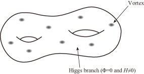
(a) Small size vortices ($g_{0}^{2}\zeta\gg\frac{4\pi k}{{\cal A}}$)

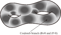
(b) Vortices near the Bradlow bound ($g_{0}^{2}\zeta\sim\frac{4\pi k}{{\cal A}}$)

Figure 1: Two different descriptions of the vortices on the Riemann surface. For the generic (small) size of the vortices ($g_{0}^{2}\zeta\gg\frac{4\pi k}{{\cal A}}$), the Higgs vacuum dominates over the Riemann surface and the Higgs branch description is valid. At the Bradlow bound ($g_{0}^{2}\zeta=\frac{4\pi k}{{\cal A}}$), the vortex size becomes large and the Coulomb branch inside the vortices occupies the whole Riemann surface. The Coulomb branch description is valid for this situation.

The localization theorem says that the path integral is independent of the coupling $g_{0}$. in the $Q$-exact action. Therefore we can tune the coupling $g_{0}$ to allow the Coulomb branch fixed point without changing the path integral results. Moreover, we can expect that the evaluation of the path integral (the partition functions or vevs of the cohomological operators) in the two different parameter regions gives the same answer, i.e., for the partition function, we obtain

$${\cal Z}_{k}^{\text{Higgs}}(g_{0}>g_{c})={\cal Z}_{k}^{\text{Coulomb}}(g_{0}=g_{c}).$$ (4.13)

(See Fig. 2.)

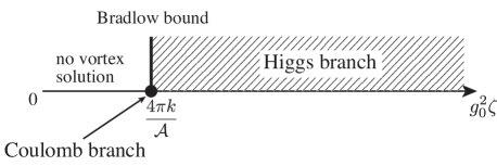
Figure 2: Complementary descriptions of the Higgs and Coulomb branches with respect to the gauge coupling and FI parameter (vortex size) $g_{0}^{2}\zeta$. In the general coupling region, the Higgs branch description is valid, but the Coulomb branch arises on the whole Riemann surface when the Bradlow bound is saturated. Using the coupling independence of the localization theorem, the evaluations of the path integral are equivalent to each other and we can use the Coulomb branch description at the extreme couplings, instead of the Higgs branch localization.

Thus, we can use the extreme Coulomb branch description of the path integral instead of the Higgs branch. A similar complementarity of two descriptions between the Higgs and Coulomb branches through the FI parameters is also discussed in the quiver quantum mechanics [27, 28].

In the following, we first discuss the Higgs branch description, but we will see that it is difficult to evaluate the path integral concretely in the Higgs branch. We will also see that the Coulomb branch description makes the evaluation of the path integral easy. This equivalence of two different descriptions is our key point of the calculation of the volume of the vortex.

4.2 Gauge fixing

Since our model has $U({N_{\rm C}})$ gauge symmetry, we need to fix the gauge symmetry in the quantization. We adopt the Becchi, Rouet, Stora and Tyutin (BRST) formalism to fix the gauge symmetry.

Introducing the Faddeev-Popov (FP) ghosts $C$ and $\bar{C}$ and the Nakanishi-Lautrup (NL) field $B$, which are in the adjoint representation, we define the BRST transformations

$$\begin{array}[]{lcl}\delta_{B}C=iC^{2},\\ \delta_{B}\bar{C}=2iB,&&\delta_{B}B=0.\end{array}$$

The BRST transformation acts on the fields as the gauge transformation with replacing the gauge transformation parameter by $C$

$$\begin{array}[]{l}\delta_{B}A_{\mu}=-\mathscr{D}_{\mu}C,\\ \delta_{B}\Phi=i[C,\Phi],\\ \delta_{B}H=iCH,\\ \text{etc.}\end{array}$$

Note that the BRST transformation is nilpotent $\delta_{B}^{2}=0$ as usual.

Once the gauge fixing function $f(A_{\mu},\Phi,\bar{\Phi},H,H^{\dagger},B)$ is given, a Lagrangian of the gauge fixing term and FP term can be written in the $\delta_{B}$-exact form

$${\cal L}_{\text{GF+FP}}=\frac{i}{g_{0}^{2}}\delta_{B}\operatorname{Tr}\left(\bar{C}f\right).$$

The BRST symmetry of the above Lagrangian is apparent from the nilpotency of $\delta_{B}$, but this gauge fixing condition violates the supersymmetry. Similarly to the supersymmetry transformation in the Wess-Zumino gauge, this phenomenon suggests that we need to supplement the supersymmetry transformation by a compensating transformation associated with the gauge transformation in order to pull the field configuration back to the gauge fixing subspace. For that purpose, we consider a linear combination of the supercharge $Q$ and the BRST transformation $\delta_{B}$, as $Q_{B}\equiv Q+i\delta_{B}$ [14]. We find that the modified supercharge $Q_{B}$ becomes nilpotent, namely $Q_{B}^{2}=0$, provided that we make an additional assumption for the supersymmetry transformation of the ghost field

$$QC=\Phi,$$

and $Q\bar{C}=QB=0$.

Using $Q_{B}$, we now introduce the total gauge fixed Lagrangian replacing the Lagrangian of $S_{0}$ in eq. (4.2)

$$\tilde{{\cal L}}\equiv Q_{B}\left[\frac{1}{g_{0}^{2}}V_{v}+V_{c}+\frac{1}{g_{0}^{2}}\operatorname{Tr}\left(\bar{C}f\right)\right],$$ (4.14)

as a $Q_{B}$ exact form. Since $V_{v}$ and $V_{c}$ are gauge (BRST) and $Q$ invariant functions of the fields, this Lagrangian reduces to

$$\begin{split}\tilde{{\cal L}}&=Q\left[\frac{1}{g_{0}^{2}}V_{v}+V_{c}\right]+\frac{i}{g_{0}^{2}}\delta_{B}\operatorname{Tr}\left(\bar{C}f\right)+\frac{1}{g_{0}^{2}}Q\operatorname{Tr}\left(\bar{C}f\right)\\ &={\cal L}_{0}+{\cal L}_{\text{GF+FP}}+\frac{1}{g_{0}^{2}}\operatorname{Tr}\left[\bar{C}(Qf)\right],\end{split}$$

using the definition of $Q_{B}$. The first and second terms are the ordinary gauge fixed Lagrangian in the BRST formalism. The extra last term $\operatorname{Tr}\left(\bar{C}Qf\right)$ can be neglected, since it can be absorbed by a shift of a field $\eta$ with a suitable choice of the gauge fixing function $f$, as we will see in the next subsection.

Since the total Lagrangian is written in the exact form of the nilpotent operator $Q_{B}$ and the measure is invariant under the $Q_{B}$-symmetry, we can conclude that the path integral is invariant under the rescaling of the overall coupling

$$\tilde{\cal L}\to t\tilde{\cal L}.$$

Thus we can use the localization arguments again for the total gauge fixed Lagrangian. Hence we consider the localization for the $Q_{B}$-exact action instead of $Q$.

4.3 Evaluation of the 1-loop determinant

Now let us consider the 1-loop approximation of the $Q_{B}$-exact action (4.14). The additional gauge fixing term in (4.14) imposes the gauge fixing condition, but the localization fixed points do not change from the original one in the $Q$-exact action. In particular, the fixed points are given by solutions of the moment map constraints, i.e., the vortex equations

$$\mu_{r}=\mu_{z}=\mu_{\bar{z}}=0.$$

In the Higgs branch, we have fixed points of $\Phi=\bar{\Phi}=0$, since the solution of the vortex equation gives $H\neq 0$ in general. Once we obtain the classical solution, we expand the fields around the fixed points by

$$\begin{split}A_{\mu}&=\hat{A}_{\mu}+\frac{1}{\sqrt{t}}\tilde{A}_{\mu},\\ H&=\hat{H}+\frac{1}{\sqrt{t}}\tilde{H},\end{split}$$

where hat fields denote a classical solution, which satisfies the moment map constraints (vortex equations), and tilde fields are fluctuations around them. Similarly we also need to expand other fields around the zeros, but it is just a rescaling of the fields like $\Phi\to\frac{1}{\sqrt{t}}\tilde{\Phi}$, $Y\to\frac{1}{\sqrt{t}}\tilde{Y}$, $\psi\to\frac{1}{\sqrt{t}}\tilde{\psi}$, etc. We will omit the tilde for these rescaled fields including the FP ghosts and NL field for simplicity in the following.

Using this expansion (rescaling) of the fields, we also expand the rescaled total Lagrangian up to the quadratic order of the fluctuations,

$$t{\cal L}_{B}=\frac{1}{g_{0}^{2}}\operatorname{Tr}\Bigg{[}\frac{1}{2}\Phi(-\hat{\mathscr{D}}^{\mu}\hat{\mathscr{D}}_{\mu}+g_{0}^{2}\hat{H}\hat{H}^{\dagger})\bar{\Phi}+\frac{1}{2}\bar{\Phi}(-\hat{\mathscr{D}}^{\mu}\hat{\mathscr{D}}_{\mu}+g_{0}^{2}\hat{H}\hat{H}^{\dagger})\Phi\\ -Y^{2}+2Y\left\{-ig^{z{\bar{z}}}(\hat{\mathscr{D}}_{z}\tilde{A}_{\bar{z}}-\hat{\mathscr{D}}_{\bar{z}}\tilde{A}_{z})-\frac{g_{0}^{2}}{2}(\tilde{H}\hat{H}^{\dagger}+\hat{H}\tilde{H}^{\dagger})\right\}\\ -\frac{g_{0}^{2}}{2}g^{z{\bar{z}}}Y_{z}Y_{\bar{z}}-ig_{0}^{2}g^{{\bar{z}}z}\left\{\hat{\mathscr{D}}_{\bar{z}}\tilde{H}+i\tilde{A}_{\bar{z}}\hat{H}\right\}Y_{z}+ig_{0}^{2}g^{{\bar{z}}z}Y_{\bar{z}}\left\{\hat{\mathscr{D}}_{z}\tilde{H}^{\dagger}-i\hat{H}^{\dagger}\tilde{A}_{z}\right\}\Bigg{]}\\ +{\cal O}(1/\sqrt{t}),$$ (4.15)

for the bosonic part and

$$t{\cal L}_{F}=\frac{1}{g_{0}^{2}}\operatorname{Tr}\Bigg{[}2ig^{z{\bar{z}}}\lambda_{z}\hat{\mathscr{D}}_{\bar{z}}\eta+2ig^{{\bar{z}}z}\lambda_{\bar{z}}\hat{\mathscr{D}}_{z}\eta-g_{0}^{2}\psi\hat{H}^{\dagger}\eta-g_{0}^{2}\eta\hat{H}\bar{\psi}\\ +\chi\left\{2ig^{z{\bar{z}}}(\hat{\mathscr{D}}_{z}\lambda_{\bar{z}}-\hat{\mathscr{D}}_{\bar{z}}\lambda_{z})+g_{0}^{2}(\psi\hat{H}^{\dagger}+\hat{H}\bar{\psi})\right\}\\ +ig_{0}^{2}g^{{\bar{z}}z}\left\{\hat{\mathscr{D}}_{\bar{z}}\psi+i\lambda_{\bar{z}}\hat{H}\right\}\chi_{z}-ig_{0}^{2}g^{{\bar{z}}z}\chi_{\bar{z}}\left\{\hat{\mathscr{D}}_{z}\bar{\psi}-i\hat{H}^{\dagger}\lambda_{z}\right\}\Bigg{]}\\ +{\cal O}(1/\sqrt{t}),$$ (4.16)

for the fermionic part, where $\hat{\mathscr{D}}_{\mu}$ means that the gauge field inside the covariant derivative is classical one.

Next let us consider the gauge fixing term. To find a suitable gauge fixing function, we pay attention to the terms proportional to $\eta$:

$$\frac{2i}{g_{0}^{2}}\operatorname{Tr}\left\{\eta\left(g^{z{\bar{z}}}(\hat{\mathscr{D}}_{z}\lambda_{\bar{z}}+\hat{\mathscr{D}}_{\bar{z}}\lambda_{z})-i\frac{g_{0}^{2}}{2}(\psi\hat{H}^{\dagger}-\hat{H}\bar{\psi})\right)\right\}\\ =\frac{2i}{g_{0}^{2}}\operatorname{Tr}\left\{\eta Q\left(\hat{\mathscr{D}}^{\mu}\tilde{A}_{\mu}-i\frac{g_{0}^{2}}{2}(\tilde{H}\hat{H}^{\dagger}-\hat{H}\tilde{H}^{\dagger})\right)\right\}.$$ (4.17)

So if we adopt the gauge fixing function for the fluctuations by

$$f(\tilde{A}_{\mu},\tilde{H},\tilde{H}^{\dagger},B)=\hat{\mathscr{D}}^{\mu}\tilde{A}_{\mu}-i\frac{g_{0}^{2}}{2}(\tilde{H}\hat{H}^{\dagger}-\hat{H}\tilde{H}^{\dagger})+\frac{1}{2}B,$$ (4.18)

the extra term $\frac{1}{g_{0}^{2}}\operatorname{Tr}\left[\bar{C}(Qf)\right]$ in the $Q_{B}$-exact gauge fixing Lagrangian (4.2) can be absorbed by shifting

$$\eta\to\eta+\frac{i}{2}\bar{C},$$

without changing the path integral, as expected.

Thus we obtain the gauge fixing and FP ghost Lagrangian for the above gauge fixing function

$$\begin{split}t{\cal L}_{\text{GF+FP}}&=\frac{i}{g_{0}^{2}}\delta_{B}\operatorname{Tr}(\bar{C}f)\\ &=\operatorname{Tr}\left[-\frac{2}{g_{0}^{2}}Bf-\frac{i}{2g_{0}^{2}}C\left(-\hat{\mathscr{D}}^{\mu}\hat{\mathscr{D}}_{\mu}+g_{0}^{2}\hat{H}\hat{H}^{\dagger}\right)\bar{C}+\frac{i}{2g_{0}^{2}}\bar{C}\left(-\hat{\mathscr{D}}^{\mu}\hat{\mathscr{D}}_{\mu}+g_{0}^{2}\hat{H}\hat{H}^{\dagger}\right)C\right],\end{split}$$ (4.19)

where we have used the BRST transformation for the fluctuation

$$\begin{split}\delta_{B}\tilde{A}_{\mu}&=-\hat{\mathscr{D}}_{\mu}C,\\ \delta_{B}\tilde{H}&=iC\hat{H},\end{split}$$

since the ghost $C$ is the same order as the fluctuations.

Comparing the bosonic part of the Lagrangian (4.15) with the ghost kinetic term in (4.19), we immediately find that the 1-loop determinants for $\Phi$-$\bar{\Phi}$ and $C$-$\bar{C}$ are canceled with each other completely. Thus we can eliminate $\Phi$-$\bar{\Phi}$ and $C$-$\bar{C}$ from the Lagrangian.

For other fields, we now define sets of the bosonic and fermionic fields by

$$\begin{array}[]{lcl}\vec{\cal B}=(\tilde{A}_{\bar{z}},\tilde{H}),&&\vec{\cal Y}=(Y+iB,Y_{\bar{z}}),\\ \vec{\cal B}^{\dagger}=(\tilde{A}_{z},\tilde{H}^{\dagger})^{T},&&\vec{\cal Y}^{\dagger}=(Y-iB,Y_{z})^{T},\\ \vec{\cal F}=(\lambda_{\bar{z}},\psi),&&\vec{\cal X}=(\eta-\chi,\chi_{\bar{z}}),\\ \vec{\cal F}^{\dagger}=(\lambda_{z},\bar{\psi})^{T},&&\vec{\cal X}^{\dagger}=(\eta+\chi,\chi_{z})^{T},\end{array}$$

then the quadratic part of the Lagrangian is written simply as

$$\begin{split}t{\cal L}_{B}&=\operatorname{Tr}\left[-\frac{1}{g_{0}^{2}}|\vec{\cal Y}|^{2}+\vec{\cal Y}\hat{D}\vec{\cal B}^{\dagger}+\vec{\cal B}\hat{D}^{\dagger}\vec{\cal Y}^{\dagger}\right],\\ t{\cal L}_{F}&=\operatorname{Tr}\left[\vec{\cal X}\hat{D}\vec{\cal F}^{\dagger}+\vec{\cal F}\hat{D}^{\dagger}\vec{\cal X}^{\dagger}\right],\end{split}$$

where

$$|\vec{\cal Y}|^{2}=Y^{2}+B^{2}+\frac{g_{0}^{2}}{2}g^{z{\bar{z}}}Y_{z}Y_{\bar{z}},$$

and

$$\hat{D}\equiv\begin{pmatrix}\frac{2i}{g_{0}^{2}}g^{z{\bar{z}}}\hat{\mathscr{D}}_{\bar{z}}&-\hat{H}\\ g^{z{\bar{z}}}\hat{H}^{\dagger}&ig^{z{\bar{z}}}\hat{\mathscr{D}}_{z}\end{pmatrix},\quad\hat{D}^{\dagger}\equiv\begin{pmatrix}\frac{2i}{g_{0}^{2}}g^{z{\bar{z}}}\hat{\mathscr{D}}_{z}&g^{z{\bar{z}}}\hat{H}\\ -\hat{H}^{\dagger}&ig^{z{\bar{z}}}\hat{\mathscr{D}}_{\bar{z}}\end{pmatrix}.$$

The 1-loop determinants of non-zero modes of the bosons and fermions cancel each other completely:

$$\text{(1-loop det)}=\frac{\det^{\prime}\hat{D}^{\dagger}\hat{D}}{\det^{\prime}\hat{D}^{\dagger}\hat{D}}=1,$$

where prime stands for omitting the zero modes (eigenvalues).

The bosonic zero modes are given by solutions to the linear equations

$$\hat{D}\vec{\cal B}^{\dagger}=0,$$

i.e., $\ker\hat{D}$. Since this equation is a linearized vortex equation and $\ker\hat{D}^{\dagger}=\emptyset$ under our choice of the BPS vortex solution $\hat{A}_{\mu}$ and $\hat{H}$ we find that

$$\dim{\cal M}_{k}=\dim\ker\hat{D}.$$ (4.20)

On the other hand, the fermionic zero modes are given by the equations

$$\hat{D}\vec{\cal F}^{\dagger}=\hat{D}^{\dagger}\vec{\cal X}^{\dagger}=0.$$

As we discussed for the bosonic zero modes, we have seen $\ker\hat{D}^{\dagger}=\emptyset$ in the BPS vortex background. So we can conclude that there is no zero mode in $\vec{\cal X}^{\dagger}$, and the number of zero modes in $\vec{\cal F}^{\dagger}$ is the same as the number of bosonic zero modes, which is $\dim\ker\hat{D}$.

We need to integrate these bosonic and fermionic zero modes after integration of the non-zero modes, which gives the cancellation of the 1-loop determinant.

4.4 Volume of the moduli space

We have seen that the partition function of the fixed topological sector ${\cal Z}_{k}$ of our model itself vanishes in general due to the existence of the fermionic zero modes. As we discussed above, we expect that there exist the fermionic zero modes only in the fields $\vec{\cal F}_{1}$ and $\vec{\cal F}_{2}$, i.e., $\lambda_{\mu}$, $\psi$ and $\bar{\psi}$.

In order to obtain a meaningful quantity from ${\cal Z}_{k}$, we need to insert some operator within the path integral, which compensates the fermionic zero modes. However an arbitrary operator cannot be inserted since it spoils the localization arguments above. As mentioned before, the supersymmetric operator does not break the coupling independence, but if we want a non-trivial (non-vanishing) quantity, we have to insert a $Q$-closed but not $Q$-exact operator ($Q$-cohomological operator).

$Q$-cohomological operators are classified in terms of the descent equations [35, 22]

$$\begin{split}Q{\cal O}_{0}&=0,\\ Q{\cal O}_{1}&=d{\cal O}_{0},\\ Q{\cal O}_{2}&=d{\cal O}_{1},\end{split}$$ (4.21)

whose $n$-form operators ${\cal O}_{n}$ are given by

$$\begin{split}{\cal O}_{0}&=\operatorname{Tr}W(\Phi),\\ {\cal O}_{1}&=-i\operatorname{Tr}W^{\prime}(\Phi)\lambda,\\ {\cal O}_{2}&=\operatorname{Tr}\left\{-iW^{\prime}(\Phi)F+\frac{1}{2}W^{\prime\prime}(\Phi)\lambda\wedge\lambda\right\},\end{split}$$ (4.22)

where $W(\Phi)$ is a polynomial of $\Phi$, the one-form $\lambda\equiv\lambda_{z}dz+\lambda_{\bar{z}}d{\bar{z}}$, and the two-form $F\equiv dA+iA\wedge A$.

From the descent equation (4.21), we find that the integration of ${\cal O}_{2}$

$${\cal I}_{2}=\int_{\Sigma_{h}}{\cal O}_{2}$$

is $Q$-closed but not $Q$-exact, since $\Sigma_{h}$ is the compact Riemann surface. If we insert the exponential of this $Q$-closed operator $e^{{\cal I}_{2}}$, the zero modes in $\lambda$ are compensated at least because of the bi-linear term of $\lambda$ in ${\cal I}_{2}$. However this operator depends on the vacuum expectation value of $\Phi$ in general and changes the value of ${\cal Z}_{k}$ excluding the zero modes. This is undesirable for our purpose.

In order not to yield the extra contribution from the inserted operator, we need to modify $e^{{\cal I}_{2}}$ by adding other $Q$-closed terms to be

$$e^{\beta{\cal I}_{V}(g)}\\ =\exp\left[\beta\operatorname{Tr}\int_{\Sigma_{h}}d^{2}z\sqrt{g}\left\{\Phi\left(-ig^{z{\bar{z}}}F_{z{\bar{z}}}+\frac{g^{2}}{2}(\zeta{\bf 1}_{{N_{\rm C}}}-HH^{\dagger})\right)-g^{z{\bar{z}}}\lambda_{z}\lambda_{\bar{z}}-\frac{g^{2}}{2}\psi\bar{\psi}\right\}\right],$$ (4.23)

where $g$ is an additional coupling constant that can differ from the coupling $g_{0}$ in the $Q$-exact action $S_{0}$ in eq. (4.3). The parameter $\beta$ serves to count the dimension of the moduli space volume (the number of continuous moduli parameters). Note here that the vev of $e^{\beta{\cal I}_{V}(g)}$ explicitly depends on the parameter $\beta$ and the coupling $g$ (and also $\zeta$), since the above operator is $Q$-closed but not $Q$-exact ($Q$-cohomological), in contrast to the coupling $g_{0}$ in the $Q$-exact action. We identify this coupling $g$ in the inserted operator $e^{\beta{\cal I}_{V}(g,\zeta)}$ as the physical coupling for the BPS vortices that we study.

According to the localization theorem, the vev of the $Q$-cohomological operator can be evaluated by the solutions to the fixed point equations. As we explained before, we can evaluate the vev of the operator at any value of the gauge coupling $g_{0}$ in the $Q$-exact action $S_{0}$ in eq. (4.3), without changing the value. Evaluating the path integral in the Higgs branch, we can choose the coupling $g_{0}$ in $S_{0}$ identical to $g$ in the inserted operator $e^{\beta{\cal I}_{V}}$. Then the moment map constraint (fixed point equation) $\mu_{r}$ in eq. (3.15) becomes

$$\mu_{r}=-ig^{z{\bar{z}}}F_{z{\bar{z}}}+\frac{g}{2}(\zeta{\bf 1}_{N_{\rm C}}-HH^{\dagger})=0.$$ (4.24)

Since the solution to eq. (4.24) eliminates the factor of $\Phi$ in the exponent of $e^{\beta{\cal I}_{V}}$, the operator $e^{\beta{\cal I}_{V}}$ at $g_{0}=g$ in the Higgs branch fixed points reduces to

$$\left.e^{\beta{\cal I}_{V}(g)}\right|_{\text{Higgs branch fixed point}}=\exp\left[-\beta\operatorname{Tr}\int_{\Sigma_{h}}d^{2}z\sqrt{g}\left\{g^{z{\bar{z}}}\lambda_{z}\lambda_{\bar{z}}+\frac{g^{2}}{2}\psi\bar{\psi}\right\}\right].$$ (4.25)

The bosonic part of this operator value at the Higgs branch fixed point gives just unity, but the fermionic part compensates all the fermionic zero modes since the exponent contains bi-linear terms of fermion pairs; $(\lambda_{z},\lambda_{\bar{z}})$ and $(\psi,\bar{\psi})$. After integrating over the fermionic zero modes, only appropriate product of the fermionic pairs survives to give a power of $\beta$ with a unit coefficient. Hence the power of $\beta$ is given by a sum of the number of fermionic zero modes, namely the dimension of the moduli space because of (4.20).

Since the operator $e^{\beta{\cal I}_{V}(g)}$ does not change the bosonic part of the path integral at the Higgs branch coupling $g_{0}=g$, the path integral at the Higgs branch reduces to the integral over the classical solution of the vortex equation

$$\begin{split}\left\langle e^{\beta{\cal I}_{V}(g)}\right\rangle^{g_{0}=g}_{k}&={\cal N}\beta^{\dim_{\mathbb{C}}{\cal M}_{k}}\int\mathscr{D}\hat{A}_{\mu}\mathscr{D}\hat{H}\mathscr{D}\hat{H}^{\dagger},\end{split}$$

where $\langle\cdots\rangle^{g_{0}=g}$ stands for the evaluation of the path integral by using the $Q$-exact action with the same coupling $g_{0}=g$ as in the operator $e^{\beta{\cal I}_{V}(g)}$, $\dim_{\mathbb{C}}{\cal M}_{k}$ is a complex dimension of the moduli space of $k$ vortices, and ${\cal N}$ is a numerical constant that is associated with the normalization of the path integral measure.

Let us now rewrite the above integral in the field configuration space in terms of the moduli parameters, which parametrize the BPS vortex solution. We denote the moduli parameters by complex coordinates $m^{a}$, which span the Kähler moduli space. Changing the integral measure from the fields of $\hat{A}_{\mu}$, $\hat{H}$ and $\hat{H}^{\dagger}$, which are defined in the flat configuration space, to the moduli parameters $m^{a}$, the Jacobian factor $\det G_{a\bar{a}}(m)$ will appear, where $G_{a\bar{a}}$ is the Kähler metric of the moduli space. So we obtain

$$\begin{split}\left\langle e^{\beta{\cal I}_{V}(g)}\right\rangle_{k}^{g_{0}=g}&={\cal N}\beta^{\dim_{\mathbb{C}}{\cal M}_{k}}\int_{{\cal M}_{k}}\prod_{a=1}^{\dim_{\mathbb{C}}{\cal M}_{k}}dm^{a}d\bar{m}^{\bar{a}}\det G_{a\bar{a}}(m)\\ &={\cal N}\beta^{\dim_{\mathbb{C}}{\cal M}_{k}}\operatorname{Vol}{\cal M}_{k},\end{split}$$ (4.26)

where $\operatorname{Vol}{\cal M}_{k}$ is the volume of the $k$-vortex moduli space as we expected.

Thus we find that the path integral with the operator $e^{\beta{\cal I}_{V}(g)}$ insertion gives the volume of the moduli space. However, to evaluate the above integral, we need to know the detail of the Kähler metric $G_{a\bar{a}}$, but this is difficult in general. We see that the $\langle e^{\beta{\cal I}_{V}(g)}\rangle_{k}^{g_{0}=g}$ is proportional to the volume of the moduli space in the Higgs branch description, but we need to move into the Coulomb branch description to evaluate the volume explicitly.

Thanks to the localization theorem, we can also evaluate the above vev of the operator in the other coupling region without changing the value of the path integral, and can reach even extreme Coulomb branch couplings $g_{0}=g_{c}$, which satisfy $g_{c}^{2}\zeta=\frac{4\pi k}{{\cal A}}$. Thus we can expect equivalence between the Higgs and Coulomb branch descriptions

$$\left\langle e^{\beta{\cal I}_{V}(g)}\right\rangle^{g_{0}=g}_{k}=\left\langle e^{\beta{\cal I}_{V}(g)}\right\rangle^{g_{0}=g_{c}}_{k},$$ (4.27)

using the same cohomological operator $e^{\beta{\cal I}_{V}(g)}$, which measures the volume of the moduli space at the physical coupling $g$ for our BPS vortices. We emphasize that the evaluation of Coulomb branch path integral can be done using the $Q$-exact action $S_{0}$ with the critical coupling $g_{c}$, which differs from the physical coupling $g$ in the inserted operator $e^{\beta{\cal I}_{V}(g)}$.

5 Coulomb Branch Localization

In this section, we consider the localization at the Coulomb branch, where the fields are expanded around the fixed point solution with non-vanishing $\Phi$. In the following, we evaluate the path integral using the $Q$-exact action $S_{0}$ in eq. (4.3) with the critical coupling $g_{c}$ defined by

$$g_{c}^{2}\zeta=\frac{4\pi k}{{\cal A}},$$ (5.1)

which is different from the physical value of the coupling $g$ in the inserted operator $e^{\beta{\cal I}_{V}(g)}$.

We will discuss the general non-Abelian case, but to see an essence of the Coulomb branch localization, we first explain the Abelian case.

5.1 Abelian case

In the Abelian theory, we denote the neutral scalar field by a lowercase letter $\phi$. The fixed point equations $\partial_{\mu}\phi=0$ in eq. (4.6) and $\phi H=0$ in eq. (4.8) say that $H$ vanishes if $\phi$ is a non-vanishing constant. We denote the solution to this fixed point equation by $\phi_{0}$ (constant zero mode). The classical solution of the Abelian gauge field $a_{\mu}$ satisfies

$$\frac{i}{2\pi}\int_{\Sigma_{h}}d^{2}z(\partial_{z}a_{\bar{z}}-\partial_{\bar{z}}a_{z})=k\in{\mathbb{Z}}_{\geq 0},$$

which is fixed while integrating the fluctuations in the $k$-vortex sector.

We now expand the bosonic fields in the vector multiplet around the classical solution (fixed points) by

$$\begin{split}\phi&=\phi_{0}+\frac{1}{\sqrt{t}}\tilde{\phi},\\ A_{\mu}&=a_{\mu}+\frac{1}{\sqrt{t}}\tilde{A}_{\mu},\end{split}$$

and the auxiliary field $Y$ is also rescaled by $Y\to\frac{1}{\sqrt{t}}\tilde{Y}$.

For the fermionic fields, we expect that there are two 0-form zero modes and $2h$ 1-form zero modes on the Riemann surface with the genus $h$, since these zero modes are associated with 0th and 1st cohomology on $\Sigma_{h}$, respectively. We denote the 0-form zero modes by $\eta_{0}$, $\chi_{0}$ and 1-form zero modes by $\lambda_{0,z}=\sum_{l=1}^{h}\lambda^{(l)}_{0}\omega^{(l)}$ and $\lambda_{0,{\bar{z}}}=\sum_{l=1}^{h}\bar{\lambda}^{(l)}_{0}\bar{\omega}^{(l)}$, where $\omega^{(l)}$ and $\bar{\omega}^{(l)}$ take values in the bases of $H^{1,0}(\Sigma_{h},\mathbb{Z})$ and $H^{0,1}(\Sigma_{h},\mathbb{Z})$, respectively. The 1-form bases are normalized by

$$\int_{\Sigma_{h}}d^{2}z\,\omega^{(l)}\bar{\omega}^{(l^{\prime})}=\delta_{ll^{\prime}}.$$ (5.2)

Thus we also expand the fermionic fields in the vector multiplets around these zero modes as

$$\begin{split}\eta&=\eta_{0}+\frac{1}{\sqrt{t}}\tilde{\eta},\\ \chi&=\chi_{0}+\frac{1}{\sqrt{t}}\tilde{\chi},\\ \lambda_{\mu}&=\lambda_{0,\mu}+\frac{1}{\sqrt{t}}\tilde{\lambda}_{\mu}.\end{split}$$

In contrast to the Higgs branch evaluation, the fixed point solution of the bosonic field $H$ vanishes. So we rescale the bosons and fermions in the chiral multiplet as

$$H\to\frac{1}{\sqrt{t}}\tilde{H},\quad Y_{\mu}\to\frac{1}{\sqrt{t}}\tilde{Y}_{\mu},\quad\psi\to\frac{1}{\sqrt{t}}\tilde{\psi},\quad\chi_{\mu}=\frac{1}{\sqrt{t}}\tilde{\chi}_{\mu}.$$

This rescaling is always guaranteed by the invariance of the path integral measure

$$\mathscr{D}^{2}H\mathscr{D}^{2}Y_{\mu}\mathscr{D}^{2}\psi\mathscr{D}^{2}\chi_{\mu}.$$

Using the above expansion and rescaling, we find that the Lagrangian becomes just quadratic order in the fluctuations

$$\begin{split}t{\cal L}&=\frac{1}{g_{c}^{2}}\partial_{\mu}\tilde{\phi}\partial^{\mu}\bar{\tilde{\phi}}-\frac{1}{g_{c}^{2}}\tilde{Y}(\tilde{Y}+2ig^{z{\bar{z}}}(\partial_{z}\tilde{A}_{\bar{z}}-\partial_{\bar{z}}\tilde{A}_{z}))\\ &\qquad+2i\eta g^{z{\bar{z}}}(\partial_{z}\tilde{\lambda}_{\bar{z}}+\partial_{\bar{z}}\tilde{\lambda}_{z})-2i\chi g^{z{\bar{z}}}(\partial_{z}\tilde{\lambda}_{\bar{z}}-\partial_{\bar{z}}\tilde{\lambda}_{z})\\ &\qquad\qquad+\vec{\cal V}{\cal M}\vec{\cal V}^{\dagger}+{\cal O}(1/\sqrt{t}),\end{split}$$

where $\vec{\cal V}=(\tilde{H},\tilde{\psi},\tilde{\chi}_{\bar{z}})$, $\vec{\cal V}^{\dagger}=(\tilde{H}^{\dagger},\tilde{\bar{\psi}},\tilde{\chi}_{z})^{T}$ and

$${\cal M}=\begin{pmatrix}-2g^{z{\bar{z}}}\hat{\mathscr{D}}^{(1)}_{\bar{z}}\hat{\mathscr{D}}^{(0)}_{z}+|\phi_{0}|^{2}&-(\eta_{0}+\chi_{0})&-g^{z{\bar{z}}}\lambda_{0,{\bar{z}}}\\ -(\eta_{0}-\chi_{0})&-\bar{\phi}_{0}&-ig^{z{\bar{z}}}\hat{\mathscr{D}}^{(1)}_{\bar{z}}\\ -g^{z{\bar{z}}}\lambda_{0,z}&-ig^{z{\bar{z}}}\hat{\mathscr{D}}^{(0)}_{z}&\frac{1}{2}g^{z{\bar{z}}}\phi_{0}\end{pmatrix}.$$

The covariant derivatives $\hat{\mathscr{D}}^{(n)}_{\mu}$ are acting on the $n$-form field.

If the Lorentz gauge $\partial_{\mu}\tilde{A}^{\mu}=0$ is chosen, the gauge fixing and FP terms are given by

$$t{\cal L}_{\rm GF+FP}=\frac{i}{g_{c}^{2}}c(-\partial_{\mu}\partial^{\mu})\bar{c}-\frac{1}{g_{c}^{2}}B(B+2g^{z{\bar{z}}}(\partial_{z}\tilde{A}_{\bar{z}}+\partial_{\bar{z}}\tilde{A}_{z})).$$ (5.3)

Combining the quadratic part of the Lagrangian and the gauge fixing and FP terms, 1-loop determinants from the bosonic fields $(\tilde{\phi},\bar{\tilde{\phi}},\tilde{Y},B)$ and the fermionic fields $(c,\bar{c},\tilde{\eta},\tilde{\chi})$ completely give the same contribution and cancel each other (just giving one).

On the other hand, the 1-loop determinant from the chiral multiplets is given by

$$\frac{1}{\operatorname{Sdet}{\cal M}},$$

after integrating out the fluctuations $\vec{\cal V}$ and $\vec{\cal V}^{\dagger}$. If we use a decomposition of ${\cal M}$ by

$${\cal M}=\begin{pmatrix}A&B\\ C&D\end{pmatrix},$$

where

$$\begin{split}A&=-2g^{z{\bar{z}}}\hat{\mathscr{D}}^{(1)}_{\bar{z}}\hat{\mathscr{D}}^{(0)}_{z}+|\phi_{0}|^{2},\\ B&=\begin{pmatrix}-(\eta_{0}+\chi_{0})&-g^{z{\bar{z}}}\lambda_{0,{\bar{z}}}\end{pmatrix},\\ C&=\begin{pmatrix}-(\eta_{0}-\chi_{0})\\ -g^{z{\bar{z}}}\lambda_{0,z}\end{pmatrix},\\ D&=\begin{pmatrix}-\bar{\phi}_{0}&-ig^{z{\bar{z}}}\hat{\mathscr{D}}^{(1)}_{\bar{z}}\\ -ig^{z{\bar{z}}}\hat{\mathscr{D}}^{(0)}_{z}&\frac{1}{2}g^{z{\bar{z}}}\phi_{0}\end{pmatrix},\end{split}$$

then the superdeterminant is given by the determinants of the decompositions

$$\frac{1}{\operatorname{Sdet}{\cal M}}=\frac{\det D}{\det A}\det(1-X)=\frac{\det D}{\det A}e^{\operatorname{Tr}\log(1-X)},$$

where $X\equiv D^{-1}CA^{-1}B$.

To evaluate this determinant further, let us consider the eigenvalues of the Laplacians $\hat{\Delta}_{0}\equiv-2g^{z{\bar{z}}}\hat{\mathscr{D}}^{(1)}_{\bar{z}}\hat{\mathscr{D}}^{(0)}_{z}$ and $\hat{\Delta}_{1}\equiv-2g^{z{\bar{z}}}\hat{\mathscr{D}}^{(0)}_{z}\hat{\mathscr{D}}^{(1)}_{\bar{z}}$, which are acting on 0-form and 1-form eigenfunctions, respectively. If the 0-form eigenfunctions $g_{n}$ have non-vanishing eigenvalues, i.e.,

$$\hat{\Delta}_{0}g_{n}=\Lambda_{n}g_{n},$$

with $\Lambda_{n}\neq 0$, then there are associated 1-form eigenfunctions, which also have the same non-vanishing eigenvalues, since

$$\hat{\Delta}_{1}(\hat{\mathscr{D}}^{(0)}_{z}g_{n})=\hat{\mathscr{D}}^{(0)}_{z}\hat{\Delta}_{0}g_{n}=\Lambda_{n}(\hat{\mathscr{D}}^{(0)}_{z}g_{n}).$$

So we find

$${\rm Spec}^{\prime}\hat{\Delta}_{0}={\rm Spec}^{\prime}\hat{\Delta}_{1},$$

where the prime denotes that the zero eigenvalues are omitted. Thus, for the non-zero eigenvalue modes, the 1-loop determinants ${\det D}/{\det A}$ cancel each other

$$\frac{\det^{\prime}D}{\det^{\prime}A}=\frac{\sqrt{\prod_{n}(\Lambda_{n}+|\phi_{0}|^{2})(\Lambda_{n}+|\phi_{0}|^{2})}}{\prod_{n}(\Lambda_{n}+|\phi_{0}|^{2})}=1,$$

by the bosons and fermions.

On the other hand, for zero eigenvalue modes, there is no one-to-one correspondence between 0-forms and 1-forms. If we define the number of zero eigenvalue modes of the operator $\mathscr{D}^{(n)}_{\mu}$ by

$$n_{0}=\dim\ker\mathscr{D}_{z}^{(0)},\quad n_{1}=\dim\ker\mathscr{D}_{\bar{z}}^{(1)},$$

the zero eigenvalue modes contributes to the 1-loop determinant via

$$\frac{\det_{0}D}{\det_{0}A}=\left(\frac{(\bar{\phi}_{0})^{n_{0}}(\phi_{0})^{n_{1}}}{|\phi_{0}|^{2n_{0}}}\right)^{{N_{\rm F}}}.$$

So the 1-loop determinant reduces to

$$\begin{split}(\text{1-loop det})&=\frac{1}{\operatorname{Sdet}{\cal M}}\\ &=\left(\frac{(\bar{\phi}_{0})^{n_{0}}(\phi_{0})^{n_{1}}}{|\phi_{0}|^{2n_{0}}}\right)^{{N_{\rm F}}}\times e^{\operatorname{Tr}\log(1-X)}\\ &=\frac{1}{\phi_{0}^{{N_{\rm F}}(k+\frac{1}{2}\chi_{h})}}e^{\operatorname{Tr}\log(1-X)},\end{split}$$

where we have used the Hirzebruch-Riemann-Roch index theorem

$$n_{0}-n_{1}=k+\frac{1}{2}\chi_{h},$$ (5.4)

and the trace “$\operatorname{Tr}$” is taken over all modes and species (flavors) of the fields.

Next let us consider the contribution to the 1-loop determinant from $e^{\operatorname{Tr}\log(1-X)}$. We first expand

$$\operatorname{Tr}\log(1-X)=-\operatorname{Tr}X+\cdots,$$

then we have

$$-\operatorname{Tr}X=-2{N_{\rm F}}\operatorname{tr}\frac{1}{(\hat{\Delta}_{0}+|\phi_{0}|^{2})^{2}}\left(\phi_{0}\eta_{0}\chi_{0}+\bar{\phi}_{0}g^{z{\bar{z}}}\lambda_{0,z}\lambda_{0,{\bar{z}}}\right),$$

where “$\operatorname{tr}$” means the trace over the modes only (the sum over flavors is already taken) and we have used the fact that the terms proportional to

$$\operatorname{tr}\frac{\mathscr{D}_{\mu}^{(n)}}{(\hat{\Delta}_{0}+|\phi_{0}|^{2})^{2}},$$

in the trace part, vanish. Using the heat kernel regularization as explained in Appendix B, we can evaluate the trace of the operator:

$$\operatorname{tr}\frac{1}{(\hat{\Delta}_{0}+|\phi_{0}|^{2})^{2}}\left(\phi_{0}\eta_{0}\chi_{0}+\bar{\phi}_{0}g^{z{\bar{z}}}\lambda_{0,z}\lambda_{0,{\bar{z}}}\right)=\frac{1}{4\pi|\phi_{0}|^{2}}\left(\phi_{0}\eta_{0}\chi_{0}+\bar{\phi}_{0}\sum_{l=1}^{h}\lambda^{(l)}_{0}\bar{\lambda}^{(l)}_{0}\right)+\cdots.$$

Thus we obtain

$$\operatorname{Tr}\log(1-X)\simeq-\frac{{N_{\rm F}}}{2\pi}\left(\frac{\eta_{0}\chi_{0}}{\bar{\phi}_{0}}+\frac{\sum_{l=1}^{h}\lambda^{(l)}_{0}\bar{\lambda}^{(l)}_{0}}{\phi_{0}}\right),$$ (5.5)

at the 1-loop level.

Now we can explicitly evaluate the vacuum expectation value of the operator $e^{\beta{\cal I}_{V}(g)}$, which gives the volume of the moduli space of the vortices. First of all, we note here that $e^{\beta{\cal I}_{V}(g)}$ takes a value at the fixed point in the Coulomb branch

$$\left.e^{\beta{\cal I}_{V}(g)}\right|_{\text{Coulomb branch fixed point}}=e^{\beta\phi_{0}\left(\frac{g^{2}\zeta}{2}{\cal A}-2\pi k\right)-\beta\sum_{l=1}^{h}\lambda^{(l)}\bar{\lambda}^{(l)}},$$ (5.6)

in terms of the zero modes, where ${\cal A}$ is the area of the Riemann surface $\Sigma_{h}$. We would like to emphasize here that the coupling $g$ on the right-hand side of eq. (5.6) is the physical coupling of the vortex system whose volume can be evaluated and differs from the critical value coupling $g_{0}=g_{c}$ in the $Q$-exact action, i.e., we can generally assume

$$\frac{g^{2}\zeta}{2}{\cal A}-2\pi k\neq 0,$$ (5.7)

even in the Coulomb branch localization. We just need to insert this fixed point value into the path integral since the operator $e^{\beta{\cal I}_{V}(g)}$ is $Q$-closed. Putting together the 1-loop correction of the supersymmetric Yang-Mills action and the contribution from the operator $e^{\beta{\cal I}_{V}(g)}$, we can evaluate the vacuum expectation value of $e^{\beta{\cal I}_{V}(g)}$ by an integral over the residual zero modes of the vector multiplet

$$\begin{split}\left\langle e^{\beta{\cal I}_{V}(g)}\right\rangle^{g_{0}=g_{c}}_{k}&=\int\frac{d\phi_{0}}{2\pi i}\frac{d\bar{\phi}_{0}}{2\pi i}d\eta_{0}d\chi_{0}\prod_{l=1}^{h}d\lambda^{(l)}_{0}d\bar{\lambda}^{(l)}_{0}\frac{1}{\phi_{0}^{{N_{\rm F}}(k+\frac{1}{2}\chi_{h})}}\\ &\qquad\times\exp\left\{\beta\phi_{0}\left(\frac{g^{2}\zeta}{2}{\cal A}-2\pi k\right)-\frac{{N_{\rm F}}}{2\pi\bar{\phi}_{0}}\eta_{0}\chi_{0}-\left(\beta+\frac{{N_{\rm F}}}{2\pi\phi_{0}}\right)\sum_{l=1}^{h}\lambda^{(l)}\bar{\lambda}^{(l)}\right\},\end{split}$$ (5.8)

where we have normalized the integral measure of $\phi_{0}$ and $\bar{\phi}_{0}$, dividing by $2\pi i$. Using the evaluation of the following integral

$$\int\frac{d\bar{\phi}_{0}}{2\pi i\bar{\phi}_{0}}=\frac{1}{2},$$ (5.9)

with a suitable contour that contains a pole at the origin, the integral (5.8) reduces to a contour integral of $\phi_{0}$ only

$$\left\langle e^{\beta{\cal I}_{V}(g)}\right\rangle^{g_{0}=g_{c}}_{k}=\frac{{N_{\rm F}}}{4\pi}\int_{C}\frac{d\phi_{0}}{2\pi i}\frac{\left(\beta+\frac{{N_{\rm F}}}{2\pi\phi_{0}}\right)^{h}}{\phi_{0}^{{N_{\rm F}}(k+\frac{1}{2}\chi_{h})}}e^{\beta\phi_{0}\left(\frac{g^{2}\zeta}{2}{\cal A}-2\pi k\right)},$$ (5.10)

after integrating out all fermionic zero modes and $\bar{\phi}_{0}$. The factor $\left(\beta+\frac{{N_{\rm F}}}{2\pi\phi_{0}}\right)^{h}$ comes from the integral of the zero modes of $\lambda$ and $\bar{\lambda}$. This is a physical derivation of the observations in [29, 30].

The integrand in (5.10) contains a multiple pole at the origin $\phi_{0}=0$. If we consider a small shift of the position of the pole by

$$\phi_{0}\to\phi_{0}+\epsilon,$$

$\epsilon$ should satisfy

$$\mathfrak{Re}\,\epsilon\geq 0,$$

since the operator $e^{\beta{\cal I}_{V}(g)}$, which originally contains a factor

$$e^{-\beta\int_{\Sigma_{h}}d^{2}z\sqrt{g}\,(\Phi+\epsilon)HH^{\dagger}},$$

under the shift of $\Phi$, must converge as well as in the Higgs branch integral where $\Phi=0$.

On the other hand, in the Coulomb branch integration, the factor

$$e^{\beta(\phi_{0}+\epsilon)\left(\frac{g^{2}\zeta}{2}{\cal A}-2\pi k\right)}$$

in the integrand shows that

$$\mathfrak{Re}\,\phi_{0}<0\quad\text{or}\quad\mathfrak{Re}\,\phi_{0}>0$$

is required if $\left(\frac{g^{2}\zeta}{2}{\cal A}-2\pi k\right)$ is positive or negative respectively, when we add an integration contour at sufficiently large values of $|\phi_{0}|$ in upper or lower half plane in order to have a closed contour for the integral without changing its values.

Thus we can pick up the residues at $\phi_{0}=-\epsilon$ if and only if

$$\frac{g^{2}\zeta}{2}{\cal A}-2\pi k\geq 0.$$ (5.11)

(see also Fig.3). If $\frac{g^{2}\zeta}{2}{\cal A}-2\pi k$ is negative, the contour cannot contain the pole and then the integral vanishes. This mean that the moduli space (BPS solution) of the vortex does not exist if the condition (5.11) is not satisfied. This result is known as the Bradlow bound for the vortex [13]. The bound can be interpreted as each BPS vortex has an intrinsic finite size $4\pi/(g^{2}\zeta)$ preventing more vortices on the Riemann surface of area ${\cal A}$ than ${\cal A}g^{2}\zeta/(4\pi)$. The integral (5.8) gives the correct formula for the volume of the moduli space without explicit knowledge of the moduli space metric. It automatically gives the selection rule of integration contours leading to the Bradlow bound.

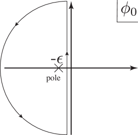
(a) $\frac{g^{2}\zeta}{2}{\cal A}-2\pi k>0$

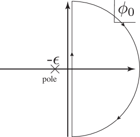
(b) $\frac{g^{2}\zeta}{2}{\cal A}-2\pi k<0$

Figure 3: The choice of contours depending on the sign of $\frac{g^{2}\zeta}{2}{\cal A}-2\pi k$. The pole is inside the contour and the volume of the moduli space exists if and only if the Bradlow bound is satisfied.

Let us give a concrete example. If we consider the vortices on the sphere ($h=0$ and $\chi_{h}=2$), the contour integral (5.10) gives

$$\left\langle e^{\beta{\cal I}_{V}(g)}\right\rangle^{g_{0}=g_{c}}_{k}=\frac{{N_{\rm F}}}{4\pi}\beta^{k{N_{\rm F}}+{N_{\rm F}}-1}\frac{\left(\frac{g^{2}\zeta}{2}{\cal A}-2\pi k\right)^{k{N_{\rm F}}+{N_{\rm F}}-1}}{(k{N_{\rm F}}+{N_{\rm F}}-1)!}.$$ (5.12)

The power of $\beta$ agrees with the complex dimension of the moduli space and we find that the volume of the moduli space for the Abelian vortex on the sphere is given by

$$\operatorname{Vol}{\cal M}^{1,{N_{\rm F}}}_{k}(S^{2};{\cal A})=\frac{\left(\frac{g^{2}\zeta}{2}{\cal A}-2\pi k\right)^{k{N_{\rm F}}+{N_{\rm F}}-1}}{(k{N_{\rm F}}+{N_{\rm F}}-1)!},$$ (5.13)

up to the irrelevant path integral constant ${\cal N}=\frac{{N_{\rm F}}}{4\pi}$. For the case of the vortices on the torus ($h=1$), we obtain

$$\left\langle e^{\beta{\cal I}_{V}(g)}\right\rangle^{g_{0}=g_{c}}_{k}=\frac{{N_{\rm F}}}{4\pi}\beta^{k{N_{\rm F}}}\frac{{N_{\rm F}}\frac{g^{2}\zeta}{4\pi}{\cal A}\left(\frac{g^{2}\zeta}{2}{\cal A}-2\pi k\right)^{k{N_{\rm F}}-1}}{(k{N_{\rm F}})!},$$ (5.14)

and

$$\operatorname{Vol}{\cal M}^{1,{N_{\rm F}}}_{k}(T^{2};{\cal A})=\frac{{N_{\rm F}}\frac{g^{2}\zeta}{4\pi}{\cal A}\left(\frac{g^{2}\zeta}{2}{\cal A}-2\pi k\right)^{k{N_{\rm F}}-1}}{(k{N_{\rm F}})!},$$ (5.15)

for $k>0$.

By setting ${N_{\rm F}}=1$, the above examples agree with [8], where the volume of the moduli space is directly computed from the metrics.

In the case of $k=0$, the contour integral represents the volume of the vacuum moduli space. In particular, the contour integral gives

$$\operatorname{Vol}{\cal M}_{0}^{1,N_{f}}(S^{2};{\cal A})=\frac{\left(\frac{g^{2}\zeta}{2}{\cal A}\right)^{{N_{\rm F}}-1}}{({N_{\rm F}}-1)!}=\operatorname{Vol}(\mathbb{C}P^{{N_{\rm F}}-1}),$$ (5.16)

which is the volume of the complex projective space with the radius $\frac{g^{2}\zeta}{4\pi}{\cal A}$, and

$$\operatorname{Vol}{\cal M}^{1,{N_{\rm F}}}_{0}(T^{2};{\cal A})=\frac{{N_{\rm F}}}{2\pi},$$ (5.17)

which is proportional to the number of isolated vacua (the Witten index).

Finally we comment on the power of $\beta$ (the dimension of the vortex moduli space). It can be found generally by rescaling of $\phi_{0}$ as $\phi_{0}\to\phi_{0}^{\prime}=\phi_{0}/\beta$ in the integral formula (5.10)

$$\left\langle e^{\beta{\cal I}_{V}(g)}\right\rangle_{k}=\frac{{N_{\rm F}}}{4\pi}\beta^{\frac{1}{2}({N_{\rm F}}-1)\chi_{h}+{N_{\rm F}}k}\int_{C}\frac{d\phi^{\prime}_{0}}{2\pi i}\frac{\left(1+\frac{{N_{\rm F}}}{2\pi\phi^{\prime}_{0}}\right)^{h}}{{\phi^{\prime}}_{0}^{{N_{\rm F}}(k+\frac{1}{2}\chi_{h})}}e^{\phi^{\prime}_{0}\left(\frac{g^{2}\zeta}{2}{\cal A}-2\pi k\right)}.$$

The integral expression here does not depend on $\beta$ any more and this agrees with the integral formula discussed in [31]. Thus the dimension of the moduli space of the Abelian vortex is given by

$$\dim_{\mathbb{C}}{\cal M}^{1,{N_{\rm F}}}_{k}(\Sigma_{h})=\frac{\chi_{h}}{2}({N_{\rm F}}-1)+{N_{\rm F}}k.$$ (5.18)

In order for the moduli space to exist, at least the dimension should be equal to or greater than zero. So the vorticity is restricted on the generic Riemann surface as

$$k\geq\max\left(0,-\frac{\chi_{h}({N_{\rm F}}-1)}{2{N_{\rm F}}}\right)=\max\left(0,\frac{(h-1)({N_{\rm F}}-1)}{{N_{\rm F}}}\right).$$ (5.19)

Note here that there is a non-trivial lower bound for the vorticity $k$ on higher genus Riemann surfaces ($\chi_{h}<0$) if ${N_{\rm F}}>1$, while the usual bound ($k\geq 0$) holds in the case of ${N_{\rm F}}=1$ or $\chi_{h}\geq 0$ ($h=0,1$). It is interesting to understand this phenomena from the point of view of the differential equations of the BPS vortex on higher genus Riemann surfaces.

5.2 Non-Abelian case

Now we generalize the above localization arguments to the non-Abelian case.

Let us consider the fixed point equation first. The fixed point equations for the non-Abelian theory are given by

$$\begin{split}&\mathscr{D}_{\mu}\Phi=[\Phi,\bar{\Phi}]=0,\\ &\mu_{r}=\mu_{\bar{z}}=\mu_{z}=0.\end{split}$$ (5.20)

Using the Weyl-Cartan bases (see Appendix A), the fixed point equations can be solved by

$$\begin{split}&\hat{\Phi}=\phi^{i}_{0}\mathtt{H}_{i},\\ &\hat{A}_{\mu}=a^{i}_{\mu}\mathtt{H}_{i},\end{split}$$

in a suitable gauge, where $\phi_{0}^{i}$ is a constant zero mode and the field strength $F^{(i)}_{z{\bar{z}}}=\partial_{z}a^{i}_{\bar{z}}-\partial_{\bar{z}}a^{i}_{z}$ gives magnetic fluxes for each $U(1)$ Cartan part

$$\frac{i}{2\pi}\int_{\Sigma_{h}}d^{2}z\sqrt{g}g^{z{\bar{z}}}F^{(i)}_{z{\bar{z}}}=k_{i}\quad(i=1,\ldots,{N_{\rm C}}),$$

which satisfies $k=\sum_{i=1}^{N_{\rm C}}k_{i}$.

We now expand fields around the solution of the fixed point equations, i.e.,

$$\begin{split}\Phi&=\hat{\Phi}+\frac{1}{\sqrt{t}}\tilde{\Phi}\\ &=\phi^{i}_{0}\mathtt{H}_{i}+\frac{1}{\sqrt{t}}\left(\tilde{\phi}^{i}\mathtt{H}_{i}+\tilde{\phi}^{\alpha}\mathtt{E}_{\alpha}\right),\\ A_{\mu}&=\hat{A}_{\mu}+\frac{1}{\sqrt{t}}\tilde{A}_{\mu}\\ &=a_{\mu}^{i}\mathtt{H}_{i}+\frac{1}{\sqrt{t}}\left(\tilde{A}_{\mu}^{i}\mathtt{H}_{i}+\tilde{A}_{\mu}^{\alpha}\mathtt{E}_{\alpha}\right).\end{split}$$ (5.21)

Similarly, the fermions are expanded around the corresponding zero modes:

$$\begin{split}\lambda_{\mu}&=\sum_{l=1}^{h}\lambda_{0,\mu}^{i,(l)}\mathtt{H}_{i}+\frac{1}{\sqrt{t}}\left(\tilde{\lambda}^{i}_{\mu}\mathtt{H}_{i}+\tilde{\lambda}_{\mu}^{\alpha}\mathtt{E}_{\alpha}\right)\\ \eta&=\eta_{0}^{i}\mathtt{H}_{i}+\frac{1}{\sqrt{t}}\left(\tilde{\eta}^{i}\mathtt{H}_{i}+\tilde{\eta}^{\alpha}\mathtt{E}_{\alpha}\right),\\ \chi&=\chi_{0}^{i}\mathtt{H}_{i}+\frac{1}{\sqrt{t}}\left(\tilde{\chi}^{i}\mathtt{H}_{i}+\tilde{\chi}^{\alpha}\mathtt{E}_{\alpha}\right).\\ \end{split}$$

Other fields (auxiliary fields $Y$ and the chiral multiplets) are expanded around zero, that means just rescaling by $1/\sqrt{t}$. We omit the tilde of the fluctuations for these fields.

Substituting the above expansion (5.21) into the Lagrangian, which is also rescaled by ${\cal L}\to t\cal{L}$, we find thanks to the overall coupling independence

$$\begin{split}t{\cal L}_{B}&=\frac{1}{g_{c}^{2}}\Bigg{[}g^{z{\bar{z}}}\left(|\partial_{z}\tilde{\phi}^{i}|^{2}+|\partial_{\bar{z}}\tilde{\phi}^{i}|^{2}\right)+\left\{g^{z{\bar{z}}}\left(\partial_{z}\tilde{A}^{i}_{\bar{z}}-\partial_{\bar{z}}\tilde{A}^{i}_{z}\right)\right\}^{2}\\ &\qquad\quad+g^{z{\bar{z}}}\left(|\hat{\mathscr{D}}_{z}\tilde{\phi}^{\alpha}-i\alpha(\phi_{0})\tilde{A}_{z}^{\alpha}|^{2}+|\hat{\mathscr{D}}_{\bar{z}}\tilde{\phi}^{\alpha}-i\alpha(\phi_{0})\tilde{A}_{\bar{z}}^{\alpha}|^{2}\right)\\ &\qquad\quad+\left\{g^{z{\bar{z}}}\left(\hat{\mathscr{D}}_{z}\tilde{A}^{\alpha}_{\bar{z}}-\hat{\mathscr{D}}_{\bar{z}}\tilde{A}^{\alpha}_{z}\right)\right\}^{2}+\frac{1}{4}|\alpha(\phi_{0})\bar{\tilde{\phi}}^{-\alpha}-\alpha(\bar{\phi}_{0})\tilde{\phi}^{\alpha}|^{2}\Bigg{]}\\ &\qquad\quad+{\cal O}(1/\sqrt{t})\end{split}$$

for the bosonic part after eliminating the auxiliary field $Y$, and

$$\begin{split}t{\cal L}_{F}&=\frac{1}{g_{c}^{2}}\Bigg{[}2g^{z{\bar{z}}}\left(\lambda^{i}_{z}\partial_{\bar{z}}\eta^{i}-\lambda^{i}_{\bar{z}}\partial_{z}\eta^{i}+\lambda^{-\alpha}_{z}\hat{\mathscr{D}}_{\bar{z}}\eta^{\alpha}-\lambda^{-\alpha}_{\bar{z}}\hat{\mathscr{D}}_{z}\eta^{\alpha}\right)\\ &\qquad\quad+2ig^{z{\bar{z}}}\alpha(\bar{\phi}_{0})\lambda_{z}^{-\alpha}\lambda_{\bar{z}}^{\alpha}+i\alpha(\phi_{0})\eta^{-\alpha}\eta^{\alpha}-i\alpha(\phi_{0})\chi^{-\alpha}\chi^{\alpha}\\ &\qquad\quad-2g^{z{\bar{z}}}\left(\chi^{i}(\partial_{z}\lambda_{\bar{z}}^{i}+\partial_{\bar{z}}\lambda_{z}^{i})+\chi^{-\alpha}(\hat{\mathscr{D}}_{z}\lambda^{\alpha}_{\bar{z}}+\hat{\mathscr{D}}_{\bar{z}}\lambda^{\alpha}_{z})\right)\Bigg{]}\\ &\qquad\quad+{\cal O}(1/\sqrt{t})\end{split}$$

for the fermionic part, where $\alpha(\phi_{0})\equiv\sum_{i}\alpha_{i}\phi_{0}^{i}$, $\hat{\mathscr{D}}_{z}\tilde{\phi}^{\alpha}\equiv\partial_{z}\tilde{\phi}^{\alpha}+i\alpha(a_{z})\tilde{\phi}^{\alpha}$, etc.

Introducing two component fermions by

$$\begin{array}[]{lcl}\Psi^{i}=(\chi^{i}-\eta^{i},-\lambda^{i}_{\bar{z}})^{T},&&\bar{\Psi}^{i}=(\chi^{i}+\eta^{i},\lambda^{i}_{z}),\\ \Psi^{\alpha}=(\chi^{\alpha}+\eta^{\alpha},-\lambda^{\alpha}_{\bar{z}})^{T},&&\bar{\Psi}^{-\alpha}=(\chi^{-\alpha}-\eta^{-\alpha},\lambda^{-\alpha}_{z}),\end{array}$$

the quadratic Lagrangian of the fermionic part is written simply by

$$t{\cal L}_{F}=\frac{1}{g_{c}^{2}}\left[\sum_{i}\bar{\Psi}^{i}\not{\partial}\Psi^{i}+\sum_{\alpha}\bar{\Psi}^{-\alpha}(\not{\mathscr{D}}-iM_{\alpha}(\phi_{0}))\Psi^{\alpha}\right]+{\cal O}(1/\sqrt{t}),$$

where

$$\not{\partial}=\begin{pmatrix}0&2g^{z{\bar{z}}}\partial_{z}\\ -2g^{z{\bar{z}}}\partial_{\bar{z}}&0\end{pmatrix},\quad\not{\mathscr{D}}=\begin{pmatrix}0&2g^{z{\bar{z}}}\hat{\mathscr{D}}_{z}\\ -2g^{z{\bar{z}}}\hat{\mathscr{D}}_{\bar{z}}&0\end{pmatrix},\quad M_{\alpha}(\phi_{0})=\begin{pmatrix}\alpha(\phi_{0})&0\\ 0&2g^{z{\bar{z}}}\alpha(\bar{\phi}_{0})\end{pmatrix}.$$

At a generic value of $\phi_{0}$, the root components of the fermions such as $\Psi^{\alpha}$ are always massive. Thus there is no true zero mode in the off-diagonal components and we expect that there are zero modes only in the Cartan part of the fermions.

Because of the supersymmetry, we can expect essentially that the 1-loop determinants reduce to one by cancellation of bosons and fermions for the non-zero modes. We should, however, pay attention to zero eigenvalue states of the operator $\hat{\mathscr{D}}_{\mu}$. According to the index theorem on the Riemann surface $\Sigma_{h}$, the numbers of the zero eigenvalue state for 0-forms and 1-forms on $\Sigma_{h}$ differ. So the contributions to 1-loop determinant from these zero eigenvalue states should not cancel each other. We call these zero eigenvalue states pseudo-zero modes.

Actually, if we evaluate the 1-loop determinant from the off-diagonal components of the pseudo-zero modes, it reduces to

$$\prod_{i\neq j}(\phi_{0}^{i}-\phi_{0}^{j})^{\frac{1}{2}\chi_{h}+k_{i}-k_{j}}=(-1)^{\sigma}\prod_{i<j}(\phi_{0}^{i}-\phi_{0}^{j})^{\chi_{h}},$$ (5.22)

where we have used the Hirzebruch-Riemann-Roch index theorem for $\not{\mathscr{D}}$ and $(-1)^{\sigma}$ is a sign factor depending on the total magnetic flux $k$ via

$$\begin{split}(-1)^{\sigma}&=(-1)^{\frac{\chi_{h}}{4}{N_{\rm C}}({N_{\rm C}}-1)-\sum_{i<j}(k_{i}-k_{j})}\\ &=\begin{cases}(-1)^{\frac{\chi_{h}}{4}{N_{\rm C}}({N_{\rm C}}-1)+k}&\text{if ${N_{\rm C}}$ is even}\\ (-1)^{\frac{\chi_{h}}{4}{N_{\rm C}}({N_{\rm C}}-1)}&\text{if ${N_{\rm C}}$ is odd}\end{cases}.\end{split}$$ (5.23)

After integrating out all off-diagonal components of the fields, the argument of the localization for each Cartan part is almost parallel to the Abelian case in the previous subsection. Using the $Q$-exactness of each Abelian component of the effective $U(1)^{N_{\rm C}}$ theory, we can vary the $i$-th $U(1)$ gauge coupling $g_{0}^{(i)}$ to be independently $g^{(i)}_{0}=g^{(i)}_{c}$ satisfying

$$(g^{(i)}_{c})^{2}\zeta=\frac{4\pi k_{i}}{{\cal A}}$$ (5.24)

Choosing the Lorentz gauge $\partial^{\mu}a^{i}_{\mu}=0$ for each $U(1)$ part, the vacuum expectation value of the operator $e^{\beta{\cal I}_{V}(g)}$ with a fixed partition of $k$ reduces to the zero mode integral

$$\begin{split}\left\langle e^{\beta{\cal I}_{V}(g)}\right\rangle^{\vec{g}_{0}=\vec{g}_{c}}_{\vec{k}}&=(-1)^{\sigma}\int\prod_{i=1}^{{N_{\rm C}}}\frac{d\phi^{i}_{0}}{2\pi i}\frac{d\bar{\phi}^{i}_{0}}{2\pi i}d\eta^{i}_{0}d\chi^{i}_{0}\prod_{l=1}^{h}d\lambda^{i,(l)}_{0}d\bar{\lambda}^{i,(l)}_{0}\frac{1}{(\phi^{i}_{0})^{{N_{\rm F}}(k_{i}+\frac{1}{2}\chi_{h})}}\prod_{i<j}(\phi_{0}^{i}-\phi_{0}^{j})^{\chi_{h}}\\ &\qquad\times\exp\left[\sum_{i=1}^{{N_{\rm C}}}\left\{\beta\phi^{i}_{0}\left(\frac{g^{2}\zeta}{2}{\cal A}-2\pi k_{i}\right)-\frac{{N_{\rm F}}}{2\pi i\bar{\phi}^{i}_{0}}\eta^{i}_{0}\chi^{i}_{0}-\left(\beta+\frac{{N_{\rm F}}}{2\pi\phi^{i}_{0}}\right)\sum_{l=1}^{h}\lambda^{i,(l)}_{0}\bar{\lambda}^{i,(l)}_{0}\right\}\right],\end{split}$$

where $\vec{g}_{0}=\vec{g}_{c}$ stands for $g^{(i)}_{0}=g^{(i)}_{c}$ $(i=1,\ldots,{N_{\rm C}})$ and $\vec{k}=(k_{1},\ldots,k_{N_{\rm C}})$. Here we again note that the coupling $g$ on the right-hand side coming from the inserted operator differs from the coupling $g^{(i)}_{0}=g^{(i)}_{c}$ in the $Q$-exact action. After integrating out the fermionic zero modes and $\bar{\phi}^{i}_{0}$’s, the path integral finally reduces to a contour integral formula

$$\begin{split}\left\langle e^{\beta{\cal I}_{V}(g)}\right\rangle^{\vec{g}_{0}=\vec{g}_{c}}_{\vec{k}}&=\left(\frac{{N_{\rm F}}}{4\pi}\right)^{{N_{\rm C}}}(-1)^{\sigma}\int_{C}\prod_{i=1}^{{N_{\rm C}}}\frac{d\phi^{i}_{0}}{2\pi}\prod_{i<j}(\phi_{0}^{i}-\phi_{0}^{j})^{\chi_{h}}\\ &\qquad\qquad\qquad\qquad\qquad\qquad\times\prod_{i=1}^{{N_{\rm C}}}\frac{\left(\beta+\frac{{N_{\rm F}}}{2\pi\phi^{i}_{0}}\right)^{h}}{(\phi^{i}_{0})^{{N_{\rm F}}(k_{i}+\frac{1}{2}\chi_{h})}}e^{\beta\sum_{i=1}^{{N_{\rm C}}}\phi^{i}_{0}\left(\frac{g^{2}\zeta}{2}{\cal A}-2\pi k_{i}\right)}.\end{split}$$

By summing over the partition of the total vorticity $k=\sum_{i=1}^{{N_{\rm C}}}k_{i}$ into $\vec{k}=(k_{1},k_{2},\ldots,k_{N_{\rm C}})$, we obtain the integral formula for the volume of the moduli space of the non-Abelian vortices

$$\beta^{\dim_{\mathbb{C}}{\cal M}_{k}}\operatorname{Vol}{\cal M}_{k}\\ =(-1)^{\sigma}\sum_{|\vec{k}|=k}\int_{C}\prod_{i=1}^{{N_{\rm C}}}\frac{d\phi^{i}_{0}}{2\pi i}\prod_{i<j}(\phi_{0}^{i}-\phi_{0}^{j})^{\chi_{h}}\prod_{i=1}^{{N_{\rm C}}}\frac{\left(\beta+\frac{{N_{\rm F}}}{2\pi\phi^{i}_{0}}\right)^{h}}{(\phi^{i}_{0})^{{N_{\rm F}}(k_{i}+\frac{1}{2}\chi_{h})}}e^{\beta\sum_{i=1}^{{N_{\rm C}}}\phi^{i}_{0}\left(\frac{g^{2}\zeta}{2}{\cal A}-2\pi k_{i}\right)},$$ (5.25)

up to the irrelevant numerical constant ${\cal N}\equiv\left(\frac{{N_{\rm F}}}{4\pi}\right)^{{N_{\rm C}}}$. This is the contour integral expression of the volume of the non-Abelian vortex moduli space and agrees with our previous result [31] by setting $\beta=1$.

The power of $\beta$ is also easily found by rescaling $\phi^{i}_{0}$ as $\phi^{i}_{0}\to{\phi^{\prime}}^{i}_{0}=\phi^{i}_{0}/\beta$. Using this rescaling, we find that the dimension of the moduli space of the non-Abelian vortex is generally given by

$$\begin{split}\dim_{\mathbb{C}}{\cal M}^{{N_{\rm C}},{N_{\rm F}}}_{k}(\Sigma_{h})&=\frac{\chi_{h}}{2}{N_{\rm C}}({N_{\rm F}}-{N_{\rm C}})+{N_{\rm F}}k\\ &=\frac{\chi_{h}}{2}{N_{\rm C}}\tilde{N}_{C}+({N_{\rm C}}+{\tilde{N}}_{C})k,\end{split}$$ (5.26)

where $\tilde{N}_{C}\equiv{N_{\rm F}}-{N_{\rm C}}$. It is interesting that the dimension of the moduli space (5.26) is invariant under the duality transformation ${N_{\rm C}}\leftrightarrow\tilde{N}_{C}$. The $k$-dependent part in (5.26) agrees with the result on the flat space $\mathbb{R}^{2}$ [36, 37, 3]. The positivity of the dimension leads to the lower bound of the vorticity

$$k\geq\max\left(0,(h-1)\frac{{N_{\rm C}}\tilde{N}_{C}}{{N_{\rm C}}+\tilde{N}_{C}}\right).$$ (5.27)

From the viewpoint of the BPS differential equations, it is difficult to find a topology ($\chi_{h}$) dependent part in (5.26) or (5.27), that also satisfies the duality.

5.3 Bradlow bound and Jeffrey-Kirwan residue formula

The contour integral (5.10) by $\phi_{0}$ has non-vanishing residue if and only if

$$\frac{g^{2}\zeta}{2}{\cal A}-2\pi k\geq 0.$$ (5.28)

The condition is known as the Bradlow bound which immediately follows from the BPS equations

$$\begin{split}\int_{\Sigma_{h}}d^{2}z\sqrt{g}\left(\frac{g^{2}\zeta}{2}-ig^{z{\bar{z}}}{F_{z{\bar{z}}}}\right)&=\frac{g^{2}\zeta}{2}{\cal A}-2\pi k\\ &=\frac{g^{2}}{2}\int_{\Sigma_{h}}d^{2}z\sqrt{g}\langle HH^{\dagger}\rangle\geq 0.\end{split}$$

A similar selection rule for the contour is also known as the Jeffrey-Kirwan residue formula [38], in mathematical literature, to satisfy the D-term condition

$$\langle HH^{\dagger}\rangle=\zeta.$$

The contour for the Jeffrey-Kirwan residue formula is chosen to get non-vanishing and vanishing residues if and only if $\zeta\geq 0$ and $\zeta<0$, respectively. This Jeffrey-Kirwan residue formula causes wall-crossing phenomena in supersymmetric quantum mechanics.

The Bradlow bound can be considered as a generalization of the Jeffrey-Kirwan residue formula for the effective FI parameter including the magnetic flux

$$\langle HH^{\dagger}\rangle=\zeta_{\rm eff}(k),$$

where

$$\zeta_{\rm eff}(k)=\zeta-\frac{4\pi}{g^{2}}\frac{k}{{\cal A}},$$ (5.29)

is a function of the number density of the vortex $\rho=k/{\cal A}$. The contour is chosen whether $\zeta_{\rm eff}(k)$ is positive or not.

For the non-Abelian theory, our integral formula (5.25) suggests the effective FI parameter for each Abelian part as

$$\zeta_{\rm eff}(k_{i})=\zeta-\frac{4\pi}{g^{2}}\frac{k_{i}}{{\cal A}}.$$ (5.30)

This is also a generalization of the Jeffrey-Kirwan residue formula in the non-Abelian gauge theories.

6 Generating Function

So far, we have considered the volume of the moduli space under a fixed magnetic flux $k$. We consider the generating function of the volume of the moduli space, which can be obtained by a summation over the flux $k$

$$Z_{{N_{\rm C}},{N_{\rm F}}}(q;\Sigma_{h})=\sum_{k}\beta^{\dim_{\mathbb{C}}{\cal M}_{k}}\operatorname{Vol}{\cal M}_{k}\,q^{k},$$ (6.1)

where we set $q=e^{-2\pi\tau}$. $Z_{{N_{\rm C}},{N_{\rm F}}}$ can be regarded as the field theoretical partition function (4.4) with the insertion of the operator $e^{\beta{\cal I}_{V}(g)}$. We should, however, note that the summation over $k$ in the generating function (6.1) is restricted from above by the Bradlow bound, which depends on the size ${\cal A}$ of the Riemann surface.

Under this restriction of the summation over $k$, the explicit evaluation of the generating function (6.1) is rather difficult. So we consider only the case that the area of the Riemann surface ${\cal A}$ or the physical couplings $g^{2}\zeta$ are sufficiently large, namely, cases where we can take the summation up to $k\to\infty$. This implies that we should use the integration contour to enclose the pole at $\phi_{0}=-\epsilon$ as in Fig. 3 (a). We note that we can shift the position of the pole to the left at finite distances away from the origin without modifying the result.

Let us see some concrete examples. For the Abelian theory ($G=U(1)$), the generating function is given by

$$Z_{1,{N_{\rm F}}}(q;\Sigma_{h})=\sum_{k=0}^{\infty}\int_{C}\frac{d\phi_{0}}{2\pi i}\frac{\left(\beta+\frac{{N_{\rm F}}}{2\pi\phi_{0}}\right)^{h}}{\phi_{0}^{{N_{\rm F}}(k+\frac{1}{2}\chi_{h})}}e^{2\pi\beta\phi_{0}\left(\hat{{\cal A}}-k\right)}q^{k},$$ (6.2)

where the contour $C$ is always chosen to enclose the pole at $\phi_{0}=-\epsilon$, and

$$\hat{{\cal A}}\equiv\frac{g^{2}\zeta}{4\pi}{\cal A}.$$

If we take the summation of $k$ first assuming the interchangeability of sum and integral, we obtain

$$\begin{split}Z_{1,{N_{\rm F}}}(q;\Sigma_{h})&=\int_{C}\frac{d\phi_{0}}{2\pi i}\frac{\left(\beta+\frac{{N_{\rm F}}}{2\pi\phi_{0}}\right)^{h}}{\phi_{0}^{\frac{\chi_{h}}{2}{N_{\rm F}}}}e^{2\pi\beta\phi_{0}\hat{{\cal A}}}\sum_{k=0}^{\infty}\left(\frac{q}{\phi_{0}^{N_{\rm F}}e^{2\pi\beta\phi_{0}}}\right)^{k}\\ &=\int_{C^{\prime}}\frac{d\phi_{0}}{2\pi i}\frac{\left(\beta\phi_{0}^{N_{\rm F}}+\frac{{N_{\rm F}}}{2\pi}\phi_{0}^{{N_{\rm F}}-1}\right)^{h}}{\phi_{0}^{N_{\rm F}}-qe^{-2\pi\beta\phi_{0}}}e^{2\pi\beta\phi_{0}\hat{{\cal A}}}.\end{split}$$ (6.3)

The integrand of the above contour integral has poles at zeros of the denominator, which are solutions of

$$\phi_{0}^{N_{\rm F}}-qe^{-2\pi\beta\phi_{0}}=0.$$ (6.4)

The original degenerated pole at $\phi_{0}=-\epsilon$ spreads out into ${N_{\rm F}}$ simple poles, which are distributed roughly in the range of $|q|^{1/{N_{\rm F}}}$. The integration contour $C^{\prime}$ still encloses all the above poles since we can shift the center of the poles by a (sufficiently large) finite distance $\epsilon$ away from the origin. (see Fig. 4).

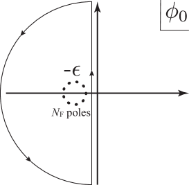
Figure 4: The integral contour of the generating function and a split of the degenerated pole. After summing up the vorticity $k$ ignoring the Bradlow bound, the degenerated pole splits into ${N_{\rm F}}$ simple poles. The integral contour still encloses all the poles since we can shift the center of the poles by sufficiently large distance $\epsilon$ against the distributions of the poles.

There is no analytical solution of the transcendental equation (6.4), but we have generally ${N_{\rm F}}$ independent solutions denoted by $x^{*}_{a}$ ($a=1,\ldots,{N_{\rm F}}$). In terms of these solutions, the contour integral (6.3) can be rewritten as

$$\begin{split}Z_{1,{N_{\rm F}}}(q;\Sigma_{h})&=\int_{C}\frac{d\phi_{0}}{2\pi i}\frac{\left(\beta\phi_{0}^{N_{\rm F}}+\frac{{N_{\rm F}}}{2\pi}\phi_{0}^{{N_{\rm F}}-1}\right)^{h}}{\prod_{a=1}^{N_{\rm F}}(\phi_{0}-x_{a}^{*})}e^{2\pi\beta\phi_{0}\hat{{\cal A}}}\\ &=\sum_{a=1}^{N_{\rm F}}\frac{\left(\beta+\frac{{N_{\rm F}}}{2\pi x_{a}^{*}}\right)^{h}}{\prod_{b\neq a}(x_{a}^{*}-x_{b}^{*})}e^{2\pi\beta x_{a}^{*}(\hat{{\cal A}}-h)}q^{h}.\end{split}$$ (6.5)

If we assume $x_{a}^{*}\ll 1$, which corresponds to $q\ll 1$ ($\tau\to\infty$), then $x^{*}_{a}$ approximately becomes

$$x^{*}_{a}\simeq\omega^{a-1}q^{1/{N_{\rm F}}},$$ (6.6)

where $\omega=\exp\left(\frac{2\pi i}{{N_{\rm F}}}\right)$ is ${N_{\rm F}}$-th root of unity. Plugging this approximation into (6.5), we obtain

$$\begin{split}Z_{1,{N_{\rm F}}}(q;\Sigma_{h})&\simeq\sum_{a=1}^{N_{\rm F}}\frac{\left(\beta+\frac{{N_{\rm F}}}{2\pi\omega^{a-1}q^{1/{N_{\rm F}}}}\right)^{h}}{\prod_{b\neq a}(\omega^{a-1}-\omega^{b-1})}e^{2\pi\beta\omega^{a-1}q^{1/{N_{\rm F}}}(\hat{{\cal A}}-h)}q^{h-\frac{{N_{\rm F}}-1}{{N_{\rm F}}}}\\ &=\sum_{j=0}^{h}\binom{h}{j}\beta^{j}\left(\frac{{N_{\rm F}}}{2\pi}\right)^{h-j}\sum_{l=1}^{\infty}\frac{1}{l!}\left(2\pi\beta(\hat{{\cal A}}-h)\right)^{l}\\ &\qquad\qquad\times\frac{1}{{N_{\rm F}}}\sum_{a=1}^{{N_{\rm F}}}\omega^{(j+l+1-h)(a-1)}q^{h-1+\frac{j+l+1-h}{{N_{\rm F}}}},\end{split}$$ (6.7)

where we have used the identity

$$\prod_{b\neq a}(\omega^{a-1}-\omega^{b-1})=\lim_{x\to\omega^{a-1}}\left(\frac{x^{N_{\rm F}}-1}{x-\omega^{a-1}}\right)=\frac{{N_{\rm F}}}{\omega^{a-1}}.$$

Because of the identity

$$\frac{1}{{N_{\rm F}}}\sum_{a=1}^{{N_{\rm F}}}\omega^{(j+l+1-h)(a-1)}=\begin{cases}1&\text{if}\quad j+l+1-h\equiv 0\pmod{{N_{\rm F}}}\\ 0&\text{otherwise}\end{cases},$$

we find that the power of $q$ in (6.7)

$$k=h-1+\frac{j+l+1-h}{{N_{\rm F}}}$$

always becomes an integer number with a bound

$$d(k)\equiv k{N_{\rm F}}-(h-1)({N_{\rm F}}-1)=j+l\geq 0,$$ (6.8)

i.e., $k\geq\max\left(-\frac{(1-h)({N_{\rm F}}-1)}{{N_{\rm F}}},0\right)$. This condition is nothing but the positivity of the dimension of the moduli space. Furthermore, using a bound

$$d(k)-j=l\geq 0,$$

we find

$$0\leq j\leq\min\left(h,d(k)\right)$$

Using these definitions and bounds, we can rewrite Eq. (6.7) as

$$\begin{split}Z_{1,{N_{\rm F}}}(q;\Sigma_{h})&=\sum_{k=k_{0}}^{\infty}\beta^{d(k)}\sum_{j=0}^{\min(h,d(k))}\binom{h}{j}\left(\frac{{N_{\rm F}}}{2\pi}\right)^{h-j}\frac{\left(2\pi(\hat{{\cal A}}-h)\right)^{d(k)-j}}{(d(k)-j)!}q^{k},\end{split}$$

where

$$k_{0}\equiv\left\lceil\frac{(h-1)({N_{\rm F}}-1)}{{N_{\rm F}}}\right\rceil,$$ (6.9)

using the ceiling function. Thus we find the volume of the moduli space

$$\beta^{\dim_{\mathbb{C}}{\cal M}_{k}}\operatorname{Vol}{\cal M}_{k}\simeq\beta^{d(k)}\sum_{j=0}^{h}\binom{h}{j}\left(\frac{{N_{\rm F}}}{2\pi}\right)^{h-j}\frac{\left(2\pi\hat{{\cal A}}\right)^{d(k)-j}}{(d(k)-j)!},$$

in the large area limit $\hat{{\cal A}}/k\to\infty$ for fixed $k$. This agrees with our previous result [31], and the power of $\beta$, $d(k)$ represents the dimension of the moduli space as we expected in the Higgs branch analysis.

Next let us consider the non-Abelian case. Ignoring the Bradlow bound, we take the summation over the vorticity first, then we have

$$\begin{split}Z_{{N_{\rm C}},{N_{\rm F}}}(q;\Sigma_{h})&=(-1)^{\frac{\chi_{h}}{4}{N_{\rm C}}({N_{\rm C}}-1)}\int_{C}\prod_{i=1}^{{N_{\rm C}}}\frac{d\phi^{i}_{0}}{2\pi i}\prod_{i<j}(\phi_{0}^{i}-\phi_{0}^{j})^{\chi_{h}}\\ &\qquad\qquad\qquad\times\prod_{i=1}^{{N_{\rm C}}}\frac{\left(\beta(\phi_{0}^{i})^{N_{\rm F}}+\frac{{N_{\rm F}}}{2\pi}(\phi_{0}^{i})^{{N_{\rm F}}-1}\right)^{h}}{(\phi^{i}_{0})^{N_{\rm F}}\mp qe^{-2\pi\beta\phi_{0}^{i}}}e^{2\pi\beta\hat{\cal A}\phi^{i}_{0}},\end{split}$$ (6.10)

where the sign in front of $q$ depends on whether ${N_{\rm C}}$ is even or odd.

Again, if we denote a set of solutions to the transcendental equation

$$(\phi^{i}_{0})^{N_{\rm F}}\mp qe^{-2\pi\beta\phi_{0}^{i}}=0,$$ (6.11)

by $x^{*}_{a}$ ($a=1,\ldots,{N_{\rm F}}$), the contour integral (6.10) is evaluated in terms of the residues

$$\begin{split}Z_{{N_{\rm C}},{N_{\rm F}}}(q;\Sigma_{h})&=(-1)^{\frac{\chi_{h}}{4}{N_{\rm C}}({N_{\rm C}}-1)}{N_{\rm C}}!\sum_{\{x^{*}_{a_{i}}\}}\prod_{i<j}(x^{*}_{a_{i}}-x^{*}_{a_{j}})^{\chi_{h}}\\ &\qquad\qquad\qquad\times\prod_{i=1}^{{N_{\rm C}}}\frac{\left(\pm\beta+\frac{{N_{\rm F}}}{2\pi x^{*}_{a_{i}}}\right)^{h}}{\prod_{a\neq a_{i}}(x^{*}_{a_{i}}-{x^{*}_{a}})}e^{2\pi\beta(\hat{\cal A}-h)x^{*}_{a_{i}}}q^{h},\end{split}$$ (6.12)

where the $a_{i}$ are a set of ${N_{\rm C}}$ indices chosen from ${N_{\rm F}}$ indices $a$, and ordered as $a_{1}<a_{2}<\cdots<a_{{N_{\rm C}}}$. (Note that we are assuming ${N_{\rm C}}\leq{N_{\rm F}}$.) This choice of indices comes from the fact that we can rearrange the order of the indices up to the Weyl permutation of the gauge group, whereas the Vandermonde determinant necessitates the choice of different poles for different $\phi_{0}^{i}$ integrals. Thus we have summation over the set of indices, whose number is given by $\binom{{N_{\rm F}}}{{N_{\rm C}}}$ in total.

It is difficult to evaluate further the expression of the volume (6.12), since the transcendental equation (6.11) does not have analytic solutions in general, but the case of ${N_{\rm C}}={N_{\rm F}}=N$ and $h=0$ ($\Sigma_{h}=S^{2}$), i.e., the non-Abelian local vortex on the sphere, is rather special. Indeed, in this case, the Vandermonde determinant is divisible by the denominator in (6.12), and it reduces to

$$Z_{N,N}(q;S^{2})=N!\,e^{2\pi\beta\hat{\cal A}\sum_{a=1}^{N}x^{*}_{a}},$$ (6.13)

where the sign factor also disappears by a cancellation with the divisor.

If we use the approximation (6.6), we cannot obtain the $q$-dependence of the generating function since $\sum_{a=1}^{N}\omega^{a-1}=0$. So we need the approximation to the next order by

$$x_{a}^{*}\simeq\omega^{a-1}(\pm q)^{1/N}e^{-2\pi/N\beta\omega^{a-1}(\pm q)^{1/N}}.$$

Using this approximation, we find

$$\begin{split}\sum_{a=1}^{N}x^{*}_{a}&\simeq\sum_{a=1}^{N}\omega^{a-1}(\pm q)^{1/N}\sum_{l=0}^{\infty}\frac{1}{l!}\left(-\frac{2\pi\beta}{N}\right)^{l}\omega^{l(a-1)}(\pm q)^{l/N}\\ &=\frac{(2\pi\beta)^{N-1}}{(N-1)!}q+{\cal O}(q^{2}).\end{split}$$

Substituting this approximation into (6.13), the generating function of the volume of the non-Abelian local vortex is given by

$$Z_{N,N}(q;S^{2})\simeq N!\times\sum_{k=0}^{\infty}\frac{1}{k!}\left\{\frac{(2\pi\beta)^{N}}{(N-1)!}\hat{{\cal A}}\right\}^{k}q^{k}.$$ (6.14)

So we find that the volume of the moduli space of the non-Abelian local vortex becomes

$$\beta^{\dim_{\mathbb{C}}{\cal M}_{k}}\operatorname{Vol}{\cal M}^{N,N}_{k}(S^{2})\simeq\frac{N!}{k!}\left\{\frac{(2\pi\beta)^{N}}{(N-1)!}\hat{{\cal A}}\right\}^{k},$$ (6.15)

in the large area limit.

This volume of the moduli space of the non-Abelian local vortex has been conjectured in eq. (4.52) of [31] by inference from the concrete evaluation for the $N=2,3$ cases, but the conjecture turns out to be in slight disagreement with our present result (6.15), which shows a slightly different coefficient. We have derived, for the general $N$, the reduction of (the dimension of) the volume of the local vortex moduli space, where the moduli space volume is proportional to $\hat{{\cal A}}^{k}$ rather than $\hat{{\cal A}}^{kN}$, by using the generating function. This is one of the advantages of using the generating function of the volume of the vortex moduli space.

7 Conclusion and Discussion

In this paper, we derive an integral formula for the volume of the moduli space of the BPS vortex on the closed Riemann surface with the arbitrary genus. The BPS vortex system is embedded into ${\cal N}{=}(2,2)$ supersymmetric Yang-Mills theory with matters, where we have used natural topological twisting on the curved space by turning on the background flux of the gauged $R$-symmetry. The background flux is compatible with the BPS vortex and preserves just half of the supercharges while the other half of the supercharges is preserved by the background for the anti-BPS vortex. This means that the zero BPS vortex sector (vacuum) on the Riemann surface differs from the zero anti-BPS vortex sector except on the torus ($h=1$).

We firstly find that the path integral of the supersymmetric Yang-Mills theory in the Higgs branch gives directly the integral over the vortex moduli space. So the partition function of the supersymmetric Yang-Mills theory essentially gives the volume of the moduli space except for the integration of fermionic zero modes. Due to the fermionic zero modes, the partition function itself vanishes. We need to insert the appropriate operator in order to obtain the moduli space volume from the path integral. The inserted operator just compensates the fermionic zero modes and reduces to unity at the localization fixed point.

Secondly, in the Higgs branch description, we cannot perform the moduli space integral since the metric of the moduli space is not known in general. However, if we evaluate the same supersymmetric system in the Coulomb branch description by using the localization method, the path integral reduces to a simple finite-dimensional contour integral, which should give the volume of the vortex moduli space as discussed in the Higgs branch description. We also derive the exact 1-loop contribution to the gaugino mass including the higher genus case, which is needed to make the effective action supersymmetric.

The localization formula for the vortex moduli space captures the effect of the finite area of the Riemann surface, known as the Bradlow bound. The choice of the contours changes whether the area and vorticity satisfy the bound or not. This can be regarded as a kind of wall-crossing or Jeffrey-Kirwan residue formula where the choice of the contour depends on the flux in general.

We also discussed the generating function of the volume of the moduli space of the vortex. Under some assumptions, we can take the summation over the vorticity first. The summation modifies the contour integral whose poles and residues are given by the transcendental equations and are difficult to obtain analytically. However, this generating function can give a simple understanding of the reduction of the moduli space dimension in the case of the local vortices (${N_{\rm C}}={N_{\rm F}}=N$).

Our volume formula for the vortex moduli space on the Riemann surface suggests that there is a lower bound of vorticity (6.9) on a Riemann surface with a higher genus ($h>1$ and ${N_{\rm F}}>{N_{\rm C}}$), besides the upper Bradlow bound. This means that there is no solution to the BPS vortex equations for too few vortices on a higher genus surface. It is interesting to understand this from the point of view of the BPS differential equations by using the moduli matrix method [3], or the Jacobian variety of the Riemann surface [39, 40].

In this paper, we consider only the case of the closed Riemann surface. If there are boundaries (punctures) of the Riemann surface, we should consider holonomies of the gauge fields around the boundaries. We expect that the partition function (the volume of the vortex moduli space) is a function of the boundary holonomies besides the vorticity and area. As known from [41], the partition function of the pure bosonic Yang-Mills theory on the arbitrary punctured Riemann surface can be constructed from those on one, two and three punctured spheres (disk, cylinder, pants) by gluing together at some boundaries. So we can expect that the volume of the vortex moduli space on the punctured Riemann surfaces may also be constructed from similar building blocks.

Our system and evaluations can be extended to three dimensions, like $S^{1}\times\Sigma_{h}$ [42, 43, 44]. The operator which measures the volume of the vortex moduli space naturally uplifts to the Chern-Simons operator in three-dimensions. So if we consider Yang-Mills-Chern-Simons-matter theory in three-dimensions, the partition function may give a counterpart of the volume of the moduli space of the vortex. After summing up the vorticity in the Yang-Mills-Chern-Simons-matter theory, the Bethe equations appear [45, 46] to determine the position of the poles in the contour integral as a generalization of our transcendental equations. In these analyses, the effects of the size of the vortices do not appear. So it is interesting to consider the dependence on the finite area ${\cal A}$ of the Riemann surface to these three-dimensional theories.

Appendix A Cartan-Weyl basis

An ${N_{\rm C}}\times{N_{\rm C}}$ matrix $X$ in the adjoint representation of $U({N_{\rm C}})$ can be expanded by the so-called Cartan-Weyl bases by

$$X=\sum_{i=1}^{{N_{\rm C}}}X^{i}\mathtt{H}_{i}+\sum_{\alpha}X^{\alpha}\mathtt{E}_{\alpha},$$

where $\alpha$ stands for the root. The Cartan-Weyl bases satisfy the following algebra

$$\begin{split}&[\mathtt{H}_{i},\mathtt{H}_{j}]=0,\\ &[\mathtt{H}_{i},\mathtt{E}_{\pm\alpha}]=\pm\alpha_{i}\mathtt{E}_{\pm\alpha},\\ &[\mathtt{E}_{\alpha},\mathtt{E}_{-\alpha}]=\sum_{i=1}^{N}\alpha_{i}\mathtt{H}_{i},\qquad[\mathtt{E}_{\alpha},\mathtt{E}_{\beta}]=N_{\alpha,\beta}\mathtt{E}_{\alpha+\beta},\\ &\mathtt{E}_{\alpha}^{\dagger}=\mathtt{E}_{-\alpha},\qquad\operatorname{Tr}\mathtt{E}_{\alpha}\mathtt{E}_{\beta}=\delta_{\alpha+\beta,0},\qquad\operatorname{Tr}\mathtt{H}_{i}\mathtt{H}_{j}=\sum_{\alpha}\alpha_{i}\alpha_{j}=\delta_{ij}.\end{split}$$ (A.1)

We use these notations in this paper.

Appendix B Heat Kernel Regularization

To compute the 1-loop contributions to the fermion bi-linears, we need to consider the contribution from the propagators in the boson-fermion loop

$$\operatorname{tr}\frac{1}{(\hat{\Delta}_{0}+|\phi_{0}|^{2})^{2}}{\cal O},$$ (B.1)

where $\hat{\Delta}_{0}\equiv-2g^{z{\bar{z}}}\hat{\mathscr{D}}^{(1)}_{z}\hat{\mathscr{D}}^{(0)}_{\bar{z}}$ is a Laplacian acting on the 0-form wave function, and ${\cal O}(z)$ is an operator. The trace is evaluated as an integral over the coordinate $z$

$$\begin{split}\operatorname{tr}\frac{1}{(\hat{\Delta}_{0}+|\phi_{0}|^{2})^{2}}{\cal O}&=\int d^{2}z\langle z|\frac{1}{(\hat{\Delta}_{0}+|\phi_{0}|^{2})^{2}}|z\rangle{\cal O}(z)\\ &=\int d^{2}z\int_{0}^{\infty}dt\,t\langle z|e^{-t(\hat{\Delta}_{0}+|\phi_{0}|^{2})}|z\rangle{\cal O}(z).\end{split}$$

We need to evaluate essentially

$$\langle z|e^{-t\hat{\Delta}_{0}}|z\rangle=\lim_{w\to z}\langle z|e^{-t\hat{\Delta}_{0}}|w\rangle,$$ (B.2)

via the heat kernel

$$h(z,w;t)=\langle z|e^{-t\hat{\Delta}_{0}}|w\rangle.$$

The heat kernel $h(z,w;t)$ obeys the heat equation

$$\left(\frac{\partial}{\partial t}+\hat{\Delta}_{0}\right)h(z,w;t)=0,$$ (B.3)

with an initial condition

$$\lim_{t\to 0}h(z,w;t)=\delta^{2}(z-w).$$

The Laplacian $\hat{\Delta}_{0}$ is defined on the curved Riemann surface and includes the spin connections, but if we expand the Laplacian around the flat-space Laplacian

$$\hat{\Delta}_{0}=-4\partial_{z}\partial_{\bar{z}}+\hat{V}_{0},$$

and treat $\hat{V}_{0}$ as a perturbation, the leading part of the heat kernel is solved to yield

$$h(z,w;t)=\frac{1}{4\pi t}e^{-|z-w|^{2}/4t}+\cdots.$$

Thus we find

$$\begin{split}\operatorname{tr}\frac{1}{(\hat{\Delta}_{0}+|\phi_{0}|^{2})^{2}}{\cal O}&=\frac{1}{4\pi}\int_{0}^{\infty}dt\,e^{-t|\phi_{0}|^{2}}\int d^{2}z\,{\cal O}(z)+\cdots\\ &=\frac{1}{4\pi}\frac{1}{|\phi_{0}|^{2}}\int d^{2}z\,{\cal O}(z)+\cdots,\end{split}$$ (B.4)

taking the limit of the trace (B.2). The higher order terms in $1/|\phi_{0}|^{2}$ contain the higher pole of $\bar{\phi}_{0}$. We only need the above leading term since these higher poles would disappear after the integration of $\bar{\phi}_{0}$.

References

• [1] E. B. Bogomolny, “Stability Of Classical Solutions,” Sov. J. Nucl. Phys.  24 (1976) 449 [Yad. Fiz.  24 (1976) 861];
• [2] M. K. Prasad and C. M. Sommerfield, “An Exact Classical Solution For The ’T Hooft Monopole And The Julia-Zee Dyon,” Phys. Rev. Lett.  35 (1975) 760.
• [3] M. Eto, Y. Isozumi, M. Nitta, K. Ohashi and N. Sakai, J. Phys. A 39, R315 (2006) doi:10.1088/0305-4470/39/26/R01 [hep-th/0602170].
• [4] E. Witten, Phys. Rev. Lett.  38, 121 (1977). doi:10.1103/PhysRevLett.38.121
• [5] N. S. Manton and N. A. Rink, J. Phys. A 43, 434024 (2010) doi:10.1088/1751-8113/43/43/434024 [arXiv:0912.2058 [hep-th]].
• [6] N. S. Manton and N. Sakai, Phys. Lett. B 687, 395 (2010) doi:10.1016/j.physletb.2010.03.017 [arXiv:1001.5236 [hep-th]].
• [7] M. Eto, T. Fujimori, M. Nitta and K. Ohashi, JHEP 1307, 034 (2013) doi:10.1007/JHEP07(2013)034 [arXiv:1207.5143 [hep-th]].
• [8] N. S. Manton and P. Sutcliffe, “Topological Solitons,” Cambridge University Press (Cabridge, UK), 2004.
• [9] N. S. Manton, Nucl. Phys.  B 400 (1993) 624.
• [10] M. Eto, T. Fujimori, M. Nitta, K. Ohashi, K. Ohta and N. Sakai, Nucl. Phys. B 788, 120 (2008) doi:10.1016/j.nuclphysb.2007.06.020 [hep-th/0703197].
• [11] T. Fujimori, G. Marmorini, M. Nitta, K. Ohashi and N. Sakai, Phys. Rev. D 82, 065005 (2010) doi:10.1103/PhysRevD.82.065005 [arXiv:1002.4580 [hep-th]].
• [12] N. S. Manton and S. M. Nasir, Commun. Math. Phys.  199, 591 (1999) doi:10.1007/s002200050513 [hep-th/9807017].
• [13] S. B. Bradlow, Commun. Math. Phys.  135, 1 (1990). doi:10.1007/BF02097654
• [14] V. Pestun et al., arXiv:1608.02952 [hep-th].
• [15] N. Hama, K. Hosomichi and S. Lee, JHEP 1103 (2011) 127 [arXiv:1012.3512 [hep-th]].
• [16] A. Kapustin, B. Willett and I. Yaakov, JHEP 1003 (2010) 089 [arXiv:0909.4559 [hep-th]].
• [17] F. Benini and S. Cremonesi, Commun. Math. Phys.  334 (2015) no.3, 1483 doi:10.1007/s00220-014-2112-z [arXiv:1206.2356 [hep-th]].
• [18] N. Doroud, J. Gomis, B. Le Floch and S. Lee, JHEP 1305 (2013) 093 doi:10.1007/JHEP05(2013)093 [arXiv:1206.2606 [hep-th]].
• [19] C. Closset and I. Shamir, JHEP 1403 (2014) 040 [arXiv:1311.2430 [hep-th]].
• [20] C. Closset, S. Cremonesi and D. S. Park, JHEP 1506 (2015) 076 doi:10.1007/JHEP06(2015)076 [arXiv:1504.06308 [hep-th]].
• [21] E. Witten, Commun. Math. Phys.  118, 411 (1988). doi:10.1007/BF01466725
• [22] E. Witten, J. Geom. Phys.  9 (1992) 303 doi:10.1016/0393-0440(92)90034-X [hep-th/9204083].
• [23] C. Closset and S. Cremonesi, JHEP 1407 (2014) 075 doi:10.1007/JHEP07(2014)075 [arXiv:1404.2636 [hep-th]].
• [24] F. Benini and A. Zaffaroni, Proc. Symp. Pure Math.  96 (2017) 13 doi:10.1090/pspum/096 [arXiv:1605.06120 [hep-th]].
• [25] G. Festuccia and N. Seiberg, JHEP 1106 (2011) 114 [arXiv:1105.0689 [hep-th]].
• [26] T. T. Dumitrescu, G. Festuccia and N. Seiberg, JHEP 1208 (2012) 141 [arXiv:1205.1115 [hep-th]].
• [27] F. Denef, JHEP 0210 (2002) 023 doi:10.1088/1126-6708/2002/10/023 [hep-th/0206072].
• [28] K. Ohta and Y. Sasai, JHEP 1602 (2016) 106 doi:10.1007/JHEP02(2016)106 [arXiv:1512.00594 [hep-th]].
• [29] G. W. Moore, N. Nekrasov and S. Shatashvili, Commun. Math. Phys.  209 (2000) 97 doi:10.1007/PL00005525 [hep-th/9712241].
• [30] A. A. Gerasimov and S. L. Shatashvili, Commun. Math. Phys.  277 (2008) 323 doi:10.1007/s00220-007-0369-1 [hep-th/0609024].
• [31] A. Miyake, K. Ohta and N. Sakai, Prog. Theor. Phys.  126, 637 (2011) doi:10.1143/PTP.126.637 [arXiv:1105.2087 [hep-th]].
• [32] A. Miyake, K. Ohta and N. Sakai, J. Phys. Conf. Ser.  343, 012107 (2012) doi:10.1088/1742-6596/343/1/012107 [arXiv:1111.4333 [hep-th]].
• [33] K. Ohta, N. Sakai and Y. Yoshida, PTEP 2013 (2013) no.7, 073B03. doi:10.1093/ptep/ptt052
• [34] B. Assel, D. Cassani and D. Martelli, JHEP 1408 (2014) 123 [arXiv:1405.5144 [hep-th]].
• [35] E. Witten, Int. J. Mod. Phys. A 6 (1991) 2775. doi:10.1142/S0217751X91001350
• [36] A. Hanany and D. Tong, JHEP 0307 (2003) 037 doi:10.1088/1126-6708/2003/07/037 [hep-th/0306150].
• [37] M. Eto, Y. Isozumi, M. Nitta, K. Ohashi and N. Sakai, Phys. Rev. Lett.  96 (2006) 161601 doi:10.1103/PhysRevLett.96.161601 [hep-th/0511088].
• [38] L. C. Jeffrey and F. C. Kirwan, Topology 34 (1995) 291 doi:10.1016/0040-9383(94)00028-J [arXiv:alg-geom/9307001].
• [39] N. S. Manton and N. M. Romao, J. Geom. Phys.  61 (2011) 1135 doi:10.1016/j.geomphys.2011.02.017 [arXiv:1010.0644 [hep-th]].
• [40] N. M. Romao, J. Singul.  6 (2012) 146. doi:10.5427/jsing.2012.6l
• [41] S. Cordes, G. W. Moore and S. Ramgoolam, Nucl. Phys. Proc. Suppl.  41 (1995) 184 doi:10.1016/0920-5632(95)00434-B [hep-th/9411210].
• [42] K. Ohta and Y. Yoshida, Phys. Rev. D 86 (2012) 105018 doi:10.1103/PhysRevD.86.105018 [arXiv:1205.0046 [hep-th]].
• [43] F. Benini and A. Zaffaroni, JHEP 1507 (2015) 127 doi:10.1007/JHEP07(2015)127 [arXiv:1504.03698 [hep-th]].
• [44] C. Closset and H. Kim, JHEP 1608 (2016) 059 doi:10.1007/JHEP08(2016)059 [arXiv:1605.06531 [hep-th]].
• [45] S. Okuda and Y. Yoshida, JHEP 1211 (2012) 146 doi:10.1007/JHEP11(2012)146 [arXiv:1209.3800 [hep-th]]; JHEP 1403 (2014) 003 doi:10.1007/JHEP03(2014)003 [arXiv:1308.4608 [hep-th]]; arXiv:1501.03469 [hep-th].
• [46] H. Kanno, K. Sugiyama and Y. Yoshida, arXiv:1806.03039 [hep-th].