Variable-step-length algorithms for a random walk: hitting probability and computation performance

Abstract

We present a comparative study of several algorithms for an in-plane random walk with a variable step. The goal is to check the efficiency of the algorithm in case where the random walk terminates at some boundary. We recently found that a finite step of the random walk produces a bias in the hitting probability and this bias vanishes in the limit of an infinitesimal step. Therefore, it is important to know how a change in the step size of the random walk influences the performance of simulations. We propose an algorithm with the most effective procedure for the step-length-change protocol.

1 Introduction

Simulation of a random walk is a very general approach in many areas of science and engineering, for example, in physics (cover of a torus [1]), biology (leukocyte migration [2]), chemistry (formation of crystal patterns [3]), health research (human growth [4]), earth science (selection of river networks [5]), and natural resources research (geostatistics [6]) to mention just a few research areas.

A random walk in a domain is simulated with a finite step, i.e., with jumps of the walker of some finite distance. The size of the jumps is irrelevant while the walker is far from the domain boundary, and there is a well-established method to speed up simulations using the large step size far away from the domain [7]. The efficient algorithm to control distance to the domain boundary is based on the marked hierarchical memory (see algorithm [8] for the lattice walk and algorithm [9] for the off-lattice walk), and a proper procedure for changing the size of the jumps when close to the domain boundary must be chosen. Realization of such algorithm for the contemporary computers with relatively big onboard memory published in  [10]. Anyway, the last jump to the boundary domain is always finite in all known methods and algorithm realizations.

It was recently found [11] that the finiteness of the size of random walk jumps produces a visible bias in the hitting probability. The walker moving in the plane from infinity hits the circle at the origin and the bias in the hitting probability depends on the angle between the position of the hitting point and the radius at which the walker starts. Fortunately, the bias vanishes in the limit of an infinitesimally small step size. This motivates the present study of the efficiency of simulations while varying the step size using different protocols. Simulating a random walk with a very small size is impractical, and some protocol for changing the size must be implemented.

In this paper, we check how different protocols can influence the simulation efficiency, minimizing the time needed to hit the boundary. We estimate numerically using different protocols the probability for in-plane random walk to hit the circle placed at origin. The probability is known exactly, and it was found in the paper [11] that the bias have maximum absolute value at zero angle (and at the angles $\pm\pi)$ with respect to the initial position of the random walk, and that the bias vanishes with vanishing jump size. In the present paper we choose the bias at zero angle as indicator of the accuracy of the estimated hitting probability.

The paper is organized as follows. In section 2, we introduce the model of the random walk in the plane and provide exact results for the termination probability. In section 3, we discuss the basic algorithm, introduce the observables to control accuracy for the hitting probability, and propose the three different protocols for the variable step of the random walk. In section 4, we present the results of the simulations. A short discussion of the results in section 5 concludes our paper.

2 Model

One of the most interesting cases for simulating a random walk is the random walk in the plane, for at least two reasons. First, it is well defined in the sense that the probability to escape to infinity is zero. The unbiased random walk is fully ergodic, it visits an $\epsilon$-neighborhood of any point in the limit of infinite time. The technical problem is that the time to reach such a neighborhood is logarithmically divergent with $\epsilon{\rightarrow}0$. Fortunately, the problem of infinite time can be eliminated because of the second reason, the existence of an exact formula for the hitting probability. The probability is defined in terms of the kernel solution of the corresponding two-dimensional Laplace equation [13, 14, 15].

We perform simulations in the following geometry. An absorbing circle of radius $R$ is placed at the origin, and the walker starts at any point on a “birth” circle of radius $R_{b}$. Walkers terminate at the absorbing circle $R$. Figure 1 schematically shows two trajectories of this type, trajectory 1–$1^{\prime}$ and trajectory 2–$2^{\prime}$.

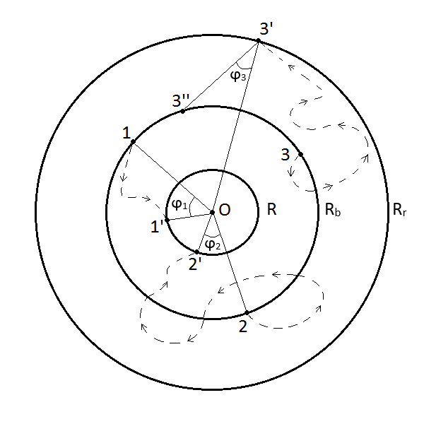
Figure 1: The random walk starts at the birth circle of radius $R_{b}$. The particle terminates when it hits the circle of radius $R$. If the particle crosses the returning circle $R_{r}$, then it is placed on the birth circle at the corresponding angle (see expression (2) and the discussion in the text).

The exact probability to hit a point on the absorbing circle $R$ is given by

$$P(\phi)=\frac{1}{2\pi}\frac{x^{2}-1}{x^{2}-2x\cos\phi+1},$$ (1)

where $x=R_{b}/R>1$ and the angle $\phi$ is measured between the radius of the initial position of the walker on the “birth” circle $R_{b}$ and the radius of the hitting point on the absorbing circle $R$. The angles $\phi_{1}$ and $\phi_{2}$ for trajectories 1–$1^{\prime}$ and 2–$2^{\prime}$ are shown in Fig. 1.

To reduce the computational time, we prevent walker from going far away: if it goes farther than the distance $R_{r}$ from the origin, then we return the walker to the birth radius at the angle $\phi$ calculated using the probability given by expression (2) with $x=R_{r}/R_{b}>1$ (see [15] for details). This case is plotted in Fig. 1 as the trajectory 3–$3^{\prime}$, which generates a walker at the point $3^{\prime\prime}$ at the radius $R_{b}$ with the angle $\phi_{3}$. The angle $\phi$ with distribution (2) is generated using the expression [13, 16, 15]

$$\phi=2\arctan\left(\frac{x-1}{x+1}\tan u\frac{\pi}{2}\right)$$ (2)

with a random variable $u$ uniformly distributed in the interval $[-1,1]$.

We must stress that this is not only a computational trick but also the way to include the infinite boundary condition exactly for the solution of the Laplace problem in the plane. Using this “killing-free” algorithm in diffusion-limited aggregation simulations, we never observe instability of the DLA cluster, which is the case in simulations in which the walker is simply removed after crossing the circle of radius $R_{r}$. The finite ratio of $R_{r}$ to $R_{b}$ leads to a distortion of the infinite boundary conditions and generates a Saffman–Taylor instability [17, 18], due to which the DLA cluster grows in only one direction [15] and develops only one of the branches.

3 Algorithm and protocols

First, we check how the accuracy of estimating the hitting probability and the computation time depends on the jump size of the random walk. We perform $N$ random walks, typically $N=10^{5}$ to $10^{6}$. For each of $N$ random walks, we generate a random angle $\phi_{0}$ uniformly distributed in $[-\pi:\pi]$ as the initial coordinate on the circle of radius $R_{b}$ (we define the direction of the angles clockwise and the value of the angles from the horizontal line). At each jump of the walk, we generate a random angle $\psi$ associated with the direction of the jump at the distance $\delta$. We calculate an estimate of the hitting probability $P_{\mathrm{sim}}(\phi)$ by dividing the interval $[-\pi:\pi]$ of possible hitting angle values $\phi$ into 180 bins and counting the number of hits for each bin. Normalizing the results over the total number $N$ of random walkers and over the bin size gives the estimate of the hitting probability $P_{\mathrm{sim}}(\phi)$. The deviation of the estimate from the exact result is calculated as

$$\Delta P(\phi)=\frac{P_{\mathrm{sim}}(\phi)-P(\phi)}{P(\phi)}.$$ (3)

Repeatedly estimating $\Delta P_{i}(\phi)$ with $N$ walkers $M$ times provides the average deviation $\Delta P_{\mathrm{av}}(\phi)$ and its standard error $D(\phi)$:

$$\Delta P_{\mathrm{av}}(\phi)=\frac{\sum_{i=1}^{M}\Delta P_{i}(\phi)}{M},$$ (4)

$$D(\phi)=\frac{\sqrt{\sum_{i=1}^{M}\left(\Delta P_{i}(\phi)-\Delta P_{\mathrm{av}}(\phi)\right)^{2}}}{M}.$$ (5)

It was observed in our previous paper [11] that i) the deviation depends on the angle $\phi$ as shown in Fig. 2 and ii) the deviation has an extremum at $\phi=0,\pm\pi$. It was proposed [11] that estimated probability does depend on the angle $\phi$ and jump size $\delta$ as

$$P_{\mathrm{sim}}(\phi)\approx P(\phi)\left(1-\left(\frac{\delta}{R}\right)^{\alpha}cos\;{\phi}\right)$$ (6)

with positive exponent $\alpha<1$.

It is visible from the Figure 2 and from the Expr. 6 that the maximum deviations occur at the angles $\phi=\pm\pi$ and 0. We choose the value $\Delta P_{\mathrm{av}}=\left|\Delta P_{\mathrm{av}}(0)\right|$ as an indicator of the accuracy of the estimated hitting probability $P_{\mathrm{sim}}(\phi)$ because it has lower dispersion in comparison with the values at the angles $\pm\pi$.

It was shown in [15] that finite-size effects are not visible for $R_{r}\gg R_{b}>R$. We therefore choose $R=10$, $R_{b}=20$, and $R_{r}=200$ in the simulations. The hitting angle was calculated at the point of intersection of the trajectory with the hitting circle $R$. For the value $R=10$ used in the simulations, for jump values limited to $\delta\leq 1$, and for the bin width $2\pi/180$, this choice of the angle does not produce a visible bias.

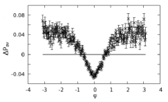
Figure 2: Deviation $\Delta P_{\mathrm{av}}(\phi)$ for the random walk step length $\delta=1$ with $M=100$.

We check three protocols.

• Equal jumps protocol. Simulations are performed with a fixed jump distance $\delta$.

• Two regions protocol. The inner space between the circles $R$ and $R_{b}$ is divided into two regions. Jumps are performed with the distance $\delta_{1}$ for a particle with the coordinate $r$ in the range $R_{c}<r<R_{r}$ and with the distance $\delta_{2}$ for a particle with $r$ in the range $R<r<R_{c}$. Accordingly, $\delta_{2}$ is taken smaller than $\delta_{1}$.

• Linear protocol. The jump size $\delta$ of the random walk is changed as a linear function of the distance $r$ to the origin:

  $$\delta(r)=\delta_{b}-(\delta_{b}-\delta_{h})\frac{R_{b}-r}{R_{b}-R}.$$ (7)

  The jump value $\delta(r)$ hence decreases from $\delta_{b}$ at the birth circle $R_{b}$ to the $\delta_{h}$ at the hitting circle $R$ and is larger than $\delta_{b}$ when the walker travels outside the birth circle $R_{b}$.

4 Simulations

4.1 Equal jumps protocol P1

The simulation results using protocol P1 are presented in Table 1, where the number in parenthesis shows the statistical uncertainty to the last digits of the quantity. The influence of the step length on the accuracy of the hitting probability is nicely demonstrated. Indeed, the data in the table shows that simulations with the smaller length size lead to better precision: a length ten times smaller gives a three times better precision. At the same time, the computation time increases by two orders of magnitude. The average number of jumps $K$ also grows drastically as the step length decreases.

Table 1: Computational performance for the equal jumps protocol P1.

$\delta$	$\Delta P_{\mathrm{av}}$	Time, min	$K$
1	0.056(2)	0.1520(4)	4814(28)
0.1	0.015(2)	14.68(3)	445359(2860)

It can be seen from Table 1 that longer jumps give better performance but a higher deviation of the hitting probability while shorter jumps give a better quality of the hitting probability and longer computation times. We must therefore find an optimum in the space of performance–accuracy. In practice, we should choose a protocol of jump length variation.

The optimal simulation should use longer jumps far from the absorbing domain and shorter jumps close to it. We consider two implementations of this idea in protocols P2 and P3.

4.2 Simple protocol P2

Protocol P2 is designed to check the idea that only final jumps influence the precision of the hitting probability. In Table 2, we show a summary of the simulations for different values of $R_{c}$, $\delta_{1}$, and $\delta_{2}$.

Table 2: Performance and precision evaluation for the simple protocol P2.

$R_{c}$	$\delta_{1}$	$\delta_{2}$	$\Delta P_{\mathrm{av}}$	$T$, min	$K$
11	1	0.3	0.024(2)	0.1559(2)	4543(29) )
	1	0.1	0.021(2)	0.1544(2)	4555(27)
	1	0.05	0.015(2)	0.1529(3)	4737(27)
	1	0.03	0.015(2)	0.1629(2)	5246(25)
	1	0.02	0.011(2)	0.1695(2)	6287(28)
	1	0.015	0.015(2)	0.1933(4)	7637(27)
	1	0.01	0.013(2)	0.2507(2)	11582(31)
15	1	0.3	0.027(2)	0.1624(2)	4983(26)
	1	0.1	0.020(2)	0.2236(2)	8351(30)
	1	0.05	0.013(2)	0.4106(6)	19878(43)
	1	0.03	0.012(2)	0.8677(5)	47027(77)
	1	0.02	0.016(2)	1.754(1)	100104(173)
	1	0.015	0.014(2)	2.874(4)	174131(312)
	1	0.01	0.014(2)	7.38(1)	386544(635)
15	5	0.3	0.027(2)	0.00976(7)	379(1)
	5	0.1	0.017(2)	0.03362(7)	1773(4)
	5	0.05	0.015(2)	0.1116(1)	6402(13)
	5	0.03	0.014(2)	0.2962(2)	17289(35)
	5	0.02	0.012(2)	0.6520(5)	38573(88)
	5	0.015	0.012(2)	1.1514(8)	67833(149)
	5	0.01	0.013(2)	2.610(2)	152715(342)

The simulation results support assumption that only the value of the last jumps are important: the deviation of the hitting probability $\Delta P_{\mathrm{av}}$ for $\delta_{2}=0.01$ is independent of the values of both the parameters $R_{c}$ and $\delta_{1}$ (compare the last row for each value of $R_{c}$). We can guess that it is reasonable to increase the value of $\delta_{1}$ as much as possible, and the limit of $\delta_{1}$ from above is $\delta_{1}\leq R_{c}-R$. For example, we cannot use values of $\delta_{1}$ larger than 1 for $R_{c}=11$ and $R=10$ or larger than 5 for $R_{c}=15$ and $R=10$ (see Table 2).

Results for $R_{c}=11$ and $\delta(r>R_{c})=5$ are missing in the table. In this case, a particle that is only 1 unit of length from the absorbing circle $R=10$ makes a jump much larger than the distance to the circle, which obviously causes huge errors in $P(\phi)$. In the simple algorithm, there is a relation between the size of the region where small jumps are made and the size of the large jump. Because we do not want the particle to jump from the region $r>R_{c}$ to the absorbing circle $R$, we should ensure that $R_{c}-R>\delta(r>R_{c})>\delta(r\leq R_{c})$. The superior choice is $R_{c}-R\gg\delta(r\leq R_{c})$, which results in a large number of steps in the region close to the absorbing circle.

One can mention inspecting Table 2, as well as the next two tables 3 and 4, that there are some minimum value of the deviation (approximately 0.013 like in the Table 2). These can be explained as the finite size effect of the finite number of bins, we use for the angle dependence of the hitting probability estimation.

4.3 Linear protocol P3

We next study the linear algorithm. Analysis of the simple algorithm shows that we can increase jump length as much as possible while keeping some region near the absorbing circle that is only accessible with small jumps. The boundary case is $\delta(r)=r-R$, which means that the particle could jump from any position in space to the absorbing sphere. We show results for the linear algorithm in Table 3.

Table 3: Performance and precision evaluation for linear protocol P3

$\delta_{b}$	$\delta_{h}$	$\Delta P_{\mathrm{av}}$	$T$, min	$K$
1	0.3	0.025(2)	0.01818(8)	787(2)
1	0.2	0.022(2)	0.01808(7)	824(2)
1	0.15	0.021(2)	0.01927(8)	865(2)
1	0.1	0.019(2)	0.01932(8)	950(2)
1	0.05	0.016(2)	0.02163(8)	1134(2)
1	0.03	0.012(2)	0.02498(8)	1281(2)
1	0.02	0.012(2)	0.02677(7)	1419(2)
1	0.01	0.010(2)	0.02950(8)	1655(3)
2	0.3	0.028(2)	0.00494(6)	219.8(5)
2	0.2	0.020(2)	0.00498(6)	240.9(5)
2	0.15	0.020(2)	0.00543(7)	257.6(5)
2	0.1	0.015(2)	0.00559(6)	283.5(5)
2	0.05	0.016(2)	0.00633(8)	336.9(6)
2	0.03	0.016(2)	0.00712(8)	378.9(5)
2	0.02	0.013(2)	0.00759(6)	414.7(6)
2	0.01	0.013(2)	0.00825(6)	477.4(6)
3	0.3	0.027(2)	0.00238(9)	107.5(2)
3	0.2	0.022(2)	0.00252(9)	117.5(2)
3	0.15	0.020(2)	0.00265(9)	126.1(2)
3	0.1	0.016(2)	0.00281(9)	139.1(3)
3	0.05	0.015(2)	0.00313(9)	163.8(3)
3	0.03	0.012(2)	0.00339(9)	183.4(3)
3	0.02	0.012(2)	0.00362(9)	199.5(3)
3	0.01	0.012(2)	0.00396(9)	226.5(3)
5	0.3	0.026(2)	0.00101(7)	42.78(7)
5	0.2	0.023(2)	0.00107(7)	46.76(8)
5	0.15	0.018(2)	0.00111(7)	49.96(8)
5	0.1	0.016(2)	0.00118(7)	54.61(9)
5	0.05	0.015(2)	0.00131(9)	63.25(9)
5	0.03	0.014(2)	0.00141(9)	69.9(1)
5	0.02	0.013(2)	0.00148(9)	75.4(1)
5	0.01	0.015(2)	0.00160(9)	84.8(1)
8	0.3	0.030(2)	0.00044(7)	16.40(3)
8	0.2	0.024(2)	0.00046(7)	17.68(3)
8	0.15	0.020(2)	0.00048(6)	18.65(3)
8	0.1	0.018(2)	0.00051(6)	20.09(3)
8	0.05	0.016(2)	0.00055(6)	22.94(3)
8	0.03	0.013(2)	0.00059(7)	24.96(3)
8	0.02	0.013(2)	0.00062(7)	26.68(3)
8	0.01	0.011(2)	0.00065(7)	29.70(4)
16	0.3	0.298(2)	0.00017(8)	5.51(2)
16	0.2	0.299(2)	0.00017(7)	5.50(2)
16	0.15	0.295(2)	0.00017(7)	5.53(2)
16	0.1	0.299(2)	0.00018(7)	5.53(2)
16	0.05	0.299(2)	0.00018(7)	5.53(2)
16	0.03	0.298(2)	0.00018(8)	5.51(2)
16	0.02	0.295(2)	0.00018(7)	5.56(2)
16	0.01	0.298(2)	0.00018(8)	5.54(2)

The behavior of the linear algorithm is similar to the simple one. Increasing the initial jump length $\delta(R_{b})$ gives better performance, and decreasing $\delta(R)$ gives better precision (and worse performance). It is important that the jumps increase linearly and there is no upper bound. Nevertheless, ratio $K_{\mathrm{return}}$ of trajectories that fly away and are returned to $R_{b}$ is almost constant.

4.4 Data analysis

We compare the different algorithms in Table 4, where we fixed the precision of the estimate of the hitting probability for a fair comparison.

Table 4: Comparison of algorithms with a precision equal to the precision of the fixed jump length algorithm with $\delta=0.1$

Algorithm				$\Delta P_{\mathrm{av}}$	$T$,min	Speedup
P1		$\delta=0.1$		0.015(2)	14.68(3)
P2	$R_{c}$	$\delta_{1}$	$\delta_{2}$
	11	1	0.03	0.015(2)	0.1629(2)	88
	15	1	0.01	0.014(2)	7.38(1)	2
	15	5	0.03	0.014(2)	0.2962(2)	50
P3		$\delta_{b}$	$\delta_{h}$
		1	0.05	0.016(2)	0.02163(8)	679
		2	0.1	0.015(2)	0.00559(6)	2626
		8	0.05	0.016(2)	0.00055(6)	26691

We choose the standard algorithm with $\delta=0.1$ as a reference and select results for simple and linear algorithms that are close to it. The best algorithm is the linear algorithm starting with $\delta=8$. This algorithm is 20000 times faster than the algorithm with a fixed $\delta=0.1$ and 200 times faster than the algorithm with the fixed $\delta=1$.

The data in Tables 2 and 3 can be analyzed to obtain more information about the algorithm performance. The data in the column Time in Table 2 can be fitted with a power law as a function of $\delta_{2}$ with the exponent $y$,

$$T\propto\delta_{2}^{-y},$$ (8)

and the data in the column $K$ can be fitted with a power law with the exponent $z$,

$$K\propto\delta_{2}^{-z}.$$ (9)

The fit of the data in Table 2 is presented in Table 5. It is clear that the simulation time $T$ and the number of steps increases as the second power of the inverse walk jump size $\delta_{2}$.

Table 5: Results of the fit to Eqs. (8) and (9) for the simple protocol P2.

$R_{c}$	$\delta_{1}$	$y$	$z$
11	1	2.52(2)	2.01(2)
15	1	2.047(1)	2.05(2)
15	5	1.998(1)	2.03(1)

In the same manner, we can fit the data in Table 3 for the linear algorithm (Protocol P3) by replacing $\delta_{2}$ with $\delta_{b}$:

$$T \propto \delta_{b}^{-y}$$ (10)

$$K \propto \delta_{b}^{-z}.$$

We show the results of the fit in Table 6. Comparing Tables 5 and 6, we can see the drastic difference in the power-law dependence for the simple protocol P2 and the linear protocol P3. The value of the exponents $y\approx 2$ and $z\approx 2$ seems constant and rather large in the case of the simple protocol P2. The values of the exponents for the linear protocol P3 are quite smaller and seem saturated to the small value $z\approx 0.1$ (we do not have reliable values of the exponent $y$ in this case).

Table 6: Results of the fit to Eqs. (8) and (9) for the linear protocol P3.

$\delta_{b}$	$y$	$z$
1	0.34(1)	0.307(6)
2	0.17(4)	0.174(5)
3	0.15(1)	0.132(5)
5	0.057(20)	0.098(5)
8	-	0.097(6)

5 Discussions

We have numerically estimated the error in a random walk simulation. The error is caused by the finite jump length that is not infinitesimally small compared with the size of the absorbing circle. We calculated the error as a function of the jump length $\delta$ and measured the angle-dependent probability distribution. The deviation of the angle dependence could lead to instabilities in a random cluster formation (e.g., in a DLA simulation). We also tested the performance and precision of variable-jump-length algorithms and showed that such algorithms can give a large performance improvement, as can be seen comparing expressions  (8), (9) and Table 5 with expression (4.4) and Table 6.

It should be noted that our results can be applied to the random walk only in two-dimensions. In larger dimensions, there is finite probability to escape to infinity while in two dimensions escaping probability is zero and random walk always return to the origin (despite the fact that the return time of the walk could be very large). In three dimensions, these leads to the interesting fact while looking for the probability that random walker will never be absorbed by the circle of radius $R$: the effective radius of the hitting sphere is changed linearly with the random walk jump size $\delta$. This effect was found by Ziff [19] and in more details in the series of papers [20, 21, 22]. It is not clear how these results and the ones we describe in the present paper are connected.

6 Acknowledgments

This work has been initiated under the grant 14-21-00158 from Russian Science Foundation and finished within the ITP Landau research subject 0033-2019-0007.

References

- [1] P. Grassberger, How fast does a random walk cover a torus? Phys. Rev. E 96 012115 (2017).
- [2] P. J. M. Jones et al., Inference of random walk models to describe leukocyte migration, Phys. Biol. 12, 066001 (2015).
- [3] R. Srivastava, N. Yadav, and J. Chattopadhyay, Growth and form of self-organized branched crystal pattern in nonlinear chemical system, in the series SpringerBriefs in Molecular Science, (Springer, 2016).
- [4] B. Suki and U. Frey, A time-varying biased random walk approach to human growth, Scientific Reports 7 , 7085 (2017).
- [5] A. Rinaldo et al., Evolution and selection of river networks: statics, dynamics, and complexity, PNAS 111, 2417-2424 (2014).
- [6] R. M. Caixeta, D. T. Ribeiro, J. F. C. L. Costa, and P. L. Machado, Multiple random walk simulation: a fast method to map grade uncertainty with large datasets, Natur. Resources Res. 26 213-221 (2017).
- [7] R.C. Ball, R.M. Brady, Large scale lattice effect in diffusion-limited aggregation, J. Phys. A 18, L809 (1985).
- [8] S. Tolman, P. Meakin, Off-lattice and hypercubic-lattice models for diffusion-limited aggregation in dimensionalities 2-8, Phys. Rev. A 40, 428 (1989).
- [9] A. Yu. Menshutin, L. N. Shchur, and V. M. Vinokour, Finite size effect of harmonic measure estimation in a DLA model: Variable size of probe particles, Physica A 387 6299-6309 (2008).
- [10] K.R. Kuijpers, L. de Martin, J. R. van Ommen, Optimizing off-lattice diffusion-limited aggregation, Comp. Phys. Comm. 185, 841 (2014).
- [11] O. Klimenkova, A. Menshutin, and L. N. Shchur, Influence of the random walk finite step on the first-passage probability, J. Phys.: Conf. Ser. 955 012009 (2018).
- [12] N. Metropolis and S. Ulam, The Monte Carlo method, Journal of the American Statistical Association 44 335 (1947).
- [13] E. Sander, L. M. Sander, and R. M. Ziff, Fractals and fractal correlations, Comput. Phys. 8, 420 (1994);
- [14] H. Kaufman, A. Vespignani, B.B. Mandelbrot, and L. Woog, Parallel diffusion-limited aggregation, Phys. Rev. E 52, 5602 (1995).
- [15] A. Yu. Menshutin and L. N. Shchur, Test of multiscaling in a diffusion-limited-aggregation model using an off-lattice killing-free algorithm, Phys. Rev. E 73, 011407 (2006).
- [16] L. M. Sander, Diffusion-limited aggregation: a kinetic critical phenomenon, Contemp. Phys. 41, 203 (2000).
- [17] P. G. Saffman and G. I. Taylor, The penetration of a fluid into a porous medium or Hele-Shaw cell containing a more viscous liquid, Proc. R. Soc. London Ser. A 245 312 (1958).
- [18] A. Leshchiner, M. Thrasher, M.B. Mineev-Weinstein, and H.L. Swinney, Harmonic moment dynamics in Laplacian growth, Phys. Rev. E 81 016206 (2010).
- [19] R. M. Ziff, Flux to a trap, J. Stat. Phys. 65, 1217 (1991).
- [20] R. M. Ziff, S. N. Majumdar, and A. Comtet, Unified solution of the expected maximum of a discrete time random walk and the discrete flux to a spherical trap, J. Stat. Phys. 122, 833 (2006).
- [21] R. M. Ziff, S. N. Majumdar, and A. Comtet, General flux to a trap in one and three dimensions, J. Phys. Cond. Mat. 19, 065102 (2007)
- [22] R. M. Ziff, S. N. Majumdar, and A. Comtet, Capture of particles undergoing discrete random walks, J. Chem. Phys. 130, 204104 (2009).