Finding high-redshift strong lenses in DES using convolutional neural networks

Abstract

We search Dark Energy Survey (DES) Year 3 imaging data for galaxy-galaxy strong gravitational lenses using convolutional neural networks. We generate 250,000 simulated lenses at redshifts > 0.8 from which we create a data set for training the neural networks with realistic seeing, sky and shot noise. Using the simulations as a guide, we build a catalogue of 1.1 million DES sources with $1.8<g-i<5$, $0.6<g-r<3$, r_mag > 19, g_mag > 20 and i_mag > 18.2. We train two ensembles of neural networks on training sets consisting of simulated lenses, simulated non-lenses, and real sources. We use the neural networks to score images of each of the sources in our catalogue with a value from 0 to 1, and select those with scores greater than a chosen threshold for visual inspection, resulting in a candidate set of 7,301 galaxies. During visual inspection we rate 84 as "probably" or "definitely" lenses. Four of these are previously known lenses or lens candidates. We inspect a further 9,428 candidates with a different score threshold, and identify four new candidates. We present 84 new strong lens candidates, selected after a few hours of visual inspection by astronomers. This catalogue contains a comparable number of high-redshift lenses to that predicted by simulations. Based on simulations we estimate our sample to contain most discoverable lenses in this imaging and at this redshift range.

1 Introduction

Gravitational lensing, a phenomenon arising from the relativistic curvature of spacetime around massive objects (Einstein, 1936; Zwicky, 1937), is a subject of increasing importance in astrophysics and cosmology. Where a large lensing potential and a close alignment of the lens mass and source coincide, strong lensing can produce highly magnified images of distant sources. When studied, they can serve as a unique probe of both lens and source properties (see Treu, 2010, for an overview). Since the detection of the first strongly lensed quasar in 1979 (Walsh et al., 1979) a growing catalogue of strong lenses has been discovered, now numbering in the hundreds.

Individual strong lenses can be highly valuable scientifically. By magnifying distant sources by a factor of tens to ~100, lensing can allow us to examine sources otherwise too distant to detect, for instance (Stark et al., 2008; Quider et al., 2009; Newton et al., 2011; Zheng et al., 2012; Ebeling et al., 2018), even a single star at redshift 1.5 (Kelly et al., 2017). In quantity, strong lenses can be valuable cosmological probes; the many applications include an independent measure of $\mbox{H}_{0}$ via time delays between multiply-imaged quasars (Bonvin et al., 2016), or testing Warm Dark Matter models through the statistics of perturbations in a large sample of Einstein rings and arcs (Vegetti et al., 2012; Li et al., 2016), including by line-of-sight substructure (Despali et al., 2018). For the latter, lenses at high redshift are particularly valuable.

Because of their high surface mass density, Early Type Galaxies (ETGs) represent the vast majority of galaxy-galaxy lenses. ETGs contain most of the stellar mass in the local universe, and so an understanding of their star formation and assembly histories is key for building an accurate picture of the evolution of structure in the universe. Strong lensing can act as a probe of lens mass with precision at great distances, and is thus a crucial tool in understanding the history of these galaxies at early times.

Observations have shown that the total density profiles of elliptical galaxies can be well-described by a power law, with $\rho(r)\propto r^{-\gamma^{\prime}}$. Observationally, most galaxies demonstrate roughly isothermal profiles, i.e. $\gamma^{\prime}\sim 2$, however reproducing the observed isothermality has proven challenging for simulations. Magneticum and EAGLE simulations both predict slopes significantly shallower than observed in local galaxies (Bellstedt et al., 2018). Simulations also predict that $\gamma^{\prime}$ becomes shallower over time (Remus et al., 2017), whilst observations suggest the opposite (Sonnenfeld et al., 2013; Shankar et al., 2018). This tension implies that our understanding of the mechanisms by which galaxies evolve, such as the role of dissipationless dry mergers at later times, is incomplete. At the present time, the redshift leverage of existing observations is insufficient to settle this question; only five lenses at redshift $>0.8$ have been available for this analysis.

Locally, the mass density profiles of ETGs have been probed using tools such as stellar dynamics (notably Tim de Zeeuw et al., 2002; Cappellari et al., 2011) and the dynamics of HI gas regions (e.g. Weijmans et al., 2008) and globular clusters (e.g. Oldham & Auger, 2018), however beyond the local universe lensing is the most practical tool. The Einstein radius of a lens system is an observable quantity and is proportional to the mass within that radius; combined with a measurement of velocity dispersion and source and lens redshifts, a robust measurement of the Einstein radius can constrain $\gamma^{\prime}$, the mean total density slope, to under five percent (Treu & Koopmans, 2004; Treu, 2010; Ruff et al., 2011). This analysis has been carried out at local redshifts, for instance by Collier et al. (2018) (two galaxies at z=0.03 and z=0.05); on 16 Sloan Lens ACS Survey (SLACS) galaxies in the redshift range 0.08 - 0.33 by Barnabè et al. (2011); and on 25 Strong Lensing Legacy Survey (SL2S) galaxies at redshifts 0.2 - 0.8 by Sonnenfeld et al. (2013), constraining $\gamma^{\prime}$ to ~5% in that range. A bigger sample of lenses at redshift $>0.8$ is needed to confirm the evolution of gamma with redshift and thereby constrain simulations and our corresponding understanding of the physics of galaxy evolution.

Finding strong lenses, especially at higher redshifts, remains a significant challenge. Currently several hundred examples of confirmed or likely galaxy-galaxy strong lenses have been discovered (Collett, 2015, the Masterlens database), with several hundred more awaiting spectroscopic or high-resolution follow up. Modelling such as (Collett, 2015) and (Treu, 2010) predicts that several thousand lenses should be detectable in current surveys such as the Dark Energy Survey (DES; The DES Collaboration, 2005) and tens of thousands in next-generation surveys such as the Large Synoptic Survey Telescope (LSST; Ivezic et al., 2008) and Euclid (Amiaux et al., 2012).

In the past, entire surveys could be searched by eye, but the data sets are now of a scale that makes this impractical. Previous strategies for automating the lens search have included searching images for characteristic features such as arcs and rings (Lenzen et al., 2004; Alard, 2006; Estrada et al., 2007; Seidel & Bartelmann, 2007; More et al., 2012; Gavazzi et al., 2014), searching for red-near-blue sources (Bolton et al., 2006; Diehl et al., 2017), applying machine learning to survey catalogs (Agnello et al., 2015), and modelling sources as lenses and testing the quality of the residual for a match (Marshall et al., 2009; Chan et al., 2015). Citizen scientists have also been recruited, with 30,000 volunteers helping to search the Canada-France-Hawaii Telescope Legacy Survey (CFHTLS) for strong lenses (Marshall et al., 2016; More et al., 2016). Some recent efforts have focused on machine learning techniques, in particular “Deep Learning”, involving the use of large Artificial Neural Networks. These techniques have already proved effective at finding lenses. Neural nets can effectively distinguish between simulated lenses and non-lenses (Jacobs et al., 2017; Lanusse et al., 2017; Avestruz et al., 2017; Hezaveh et al., 2017). Applying the technique to surveys, Jacobs et al (2017) used an ensemble of CNNs to find several hundred previously known lenses and 17 new candidates in CFHTLS in under an hour of astronomer review time, and Petrillo et al (2017) used CNNs to identify 56 new lens candidates in the Kilo Degree Survey (KiDS).

In DES, previous searches have relied heavily on the inspection of many thousands of candidates chosen from catalogue photometry; see section 5.6. Collett’s (2015) simulation suggests that approximately 8% of detectable lenses (${\sim}110$ lenses) should lie at redshifts $>0.8$. It is these lenses that are the target of the search detailed in this work.

In this paper we describe a first search for high-redshift lenses in the Dark Energy Survey using machine learning techniques. The paper is structured as follows: In section 2, we provide some brief background on the machine learning technique employed in the search, namely artificial neural networks. In section 3 we outline the methodology for constructing simulations to train the neural networks, building a catalogue of sources to search, and employing the trained networks on survey data. In section 4 we present the results of the search. In section 5 we consider ways to evaluate the performance of the lens-finding method and improve future searches, and some prospects for follow-up science and further development of the technique, the summarise our conclusions in section 6.

 

2 Artificial Neural Networks

Here we employ a machine learning technique to automatically find galaxy-galaxy strong lenses in DES image data. While traditional approaches to data problems rely on algorithms developed by subject-matter experts who define key features in the data and their relative contributions to the problem space, machine learning techniques extract features and their importance from data alone. See (Jordan & Mitchell, 2015) for an overview of the theory and applications of machine learning. Artificial Neural Networks (ANNs) are a machine learning technique first developed in the 1950s (Rosenblatt, 1957) and more heavily researched in the 1980s and 1990s (Fukushima, 1980) as non-trivial networks became computationally more tractable. ANNs are constructed to loosely mimic the structure of the brain, with a network of interconnected ‘neurons’, the strengths of the connection influencing how each neuron responds to a signal from its peers. Each artificial neuron takes an input vector; calculates the dot product with a vector of weights (i.e. real numbers that weight the contribution of each input value); and passes the resulting scalar through a non-linear function such as a logistic function or hyperbolic tangent. Neurons are arranged in layers, with an input layer at one end, an arbitrary number of “hidden layers” and an output layer interpreted appropriately to the problem domain, such as the probabilities a given input lies in one of N classes (see Figure 1). In theory, the connections between the neurons/layers can represent a highly non-linear decision boundary in many dimensions. The process of finding optimal values for the weights - the training - is data-driven (see below).

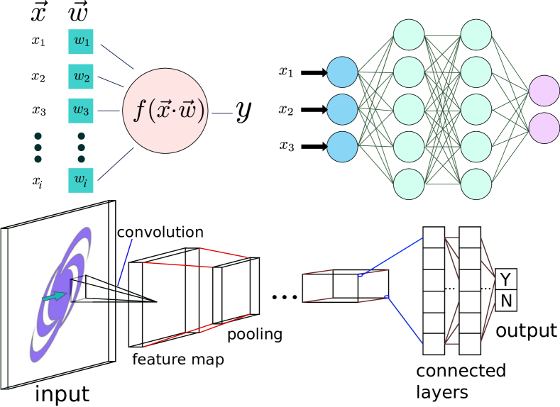
Figure 1: Overview of artificial networks. Top left: An artificial neuron. The elementwise weighted sum of a vector input is passed through a nonlinear activation function (such as the logistic function, arctangent, or rectified linear unit) to produce a scalar output. Top right: An example of a small fully-connected ANN, consisting of layers of artificial neurons. Blue: Input layer, equal in size to dimensionality of input data. Green: Hidden layers. Purple: Output layer; the outputs are interpreted according to the problem domain. Bottom: Prototypical convolutional neural network. Convolutional kernels are scanned across the input to build up so-called feature maps; pooling layers subsample the preceding layer to reduce the spatial extent. This process is repeated some number of times, then the resulting feature maps are passed to one or more fully-connected layers, followed by the output (yes/no) as the last layer.

The combination of improved technique, widely-available GPU computing, and the availability of large, labelled datasets means that large ANNs with many layers (“deep” ANNs) are now practical. This “Deep Learning” resurgence has revolutionised several fields such as computer vision and speech recognition which were able to make breakthroughs in accuracy exceeding the performance of the best hand-engineered algorithms by large margins (Schmidhuber, 2015; Guo et al., 2016).

Convolutional Neural Networks (CNNs; LeCun et al., 1989) in particular have proven highly effective at discovering patterns in image data. Unlike a standard ANN, where each layer is fully connected to the previous layer, a convolutional layer connects only small groups of neighbouring neurons, and shares the weights between groups. This has the effect of vastly reducing the number of trainable weights while at the same time taking advantage of the fact that in visual data neighbouring inputs - i.e. pixels - are highly correlated in meaningful ways. In effect, the network uses (usually square - e.g. 5x5 pixels) ‘convolutional kernels’ which are convolved with the input image or outputs of a previous layer, and act as feature detectors. Outputs are then pooled, taking the mean or maximum value of groups of pixels, reducing the spatial extent of the data as the number of feature maps increases. At earlier layers, raw features such as edges and patches of colour are detected; at later layers the network detects patterns in an increasingly abstract and high-level feature space. Thus at early layers the network activates on lines and curves; at intermediate layers on combinations of these into semantically meaningful features; then at later layers, combining these semantic features into a representation of the input in a classification space.

A CNN large enough to, for instance, distinguish between objects in hundreds of categories or decipher audio data into speech contains millions to hundreds of millions of parameters to be trained. This requires a large (i.e. up to millions of examples) training set of labelled data with which to optimise the weights to achieve the desired output semantics. The full process for training a neural network, including the backpropagation algorithm, is detailed in LeCun et al. (1998). In brief, we construct a loss function $L$ such that $L=0$ if the network classifies the training set perfectly, and increases as performance accuracy decreases. A typical loss function, and the one employed here, is a cross entropy loss function (Cao et al., 2007).

For each training example or batch of examples, and for each of the trainable weights $w_{i}$ in the network, we calculate the gradient $\delta_{i}=\partial{L}/\partial{w_{i}}$. Then, following the standard gradient descent paradigm, we update the weights by $R\delta_{i}$ where R is a free parameter, the learning rate. In this way, with each iteration the weights become more optimal to producing a low $L$ and thus more accurate classifications. Assuming a network of sufficient complexity to encode significant patterns and key features in the data, this performance will generalise to examples outside of the training set. If the dimensions of the network are not optimal, or the training set is too small, overfitting can occur where low loss is achieved on the training set but is not reflected in performance on examples not seen by the network during training. Typically, training examples are divided up into training, validation and test sets, where the training set is used to train the network and update the weights, validation is used to measure progress during training and assist in tuning parameters such as the learning rate, and the test set is reserved for a final estimate of network accuracy using labelled examples blinded from the network.

3 Method

Constructing a neural network-based system for lens-finding requires the following steps. First, we assemble training sets. Due to the limited number of known galaxy-galaxy lenses available, these consist of simulated strong lenses and non-lens systems (see section 3.2). We use the training set to iteratively train two convolutional neural networks using the Keras Deep Learning framework (Chollet, 2015) on a GPU machine. We then take a catalogue of 1.1 million sources selected to match the simulations in $g-i$ and $g-r$ colour space and evaluate postage stamp images of each galaxy with the neural networks, producing a score in the interval (0, 1) for each image. We manually examine images with scores greater than a chosen threshold and grade them 0-3, where 0 = not a lens, 1 = possibly a lens, 2 = probably a lens, and 3 = definitely a lens.

3.1 Choosing the target source population

Our science goal for the lens search is to assemble a population of lenses with measurable Einstein radii at redshifts $\gtrsim 0.8$ in order to probe their total mass profiles in this redshift range. Examining the spectral energy distribution (SED) of a typical lensing galaxy, i.e. a red, quiescent elliptical, we see that at redshift $\approx 0.8$ the rest frame UV dropoff is pushed almost entirely redward out of the DECam $g$-band filter. Thus in this redshift range we expect that a galaxy-galaxy lens with sufficient magnification to be detectable would exhibit bright source flux in the g-band but would lack a bright lens counterpart in the center of the image. This morphological hint is something we hypothesize will be utilised by the CNNs (see discussion in section 5 below).

In this section we describe the method used to choose a subset of sources in the Dark Energy Survey to search for lenses. We use catalogue values to make these cuts, then test postage stamp images of selected sources taken from DES Y3A1 coadd imaging. We restrict our search to a subset of sources in the survey catalogue for two reasons. Firstly, it reduces the amount of computational resources required, a significant consideration for a survey with around ~10TB of image data. Secondly, even a hypothetical, extremely accurate lens finder with a 0.1% false positive rate would be expected to identify 300,000 false positives across a survey of this size, a number 2-3 orders of magnitude greater than the number of lenses we expect to discover (see section 5.3). We therefore seek to increase the purity of the sample by restricting the search to sources we know are much more likely to be lenses than the average catalogued galaxy.

In catalogue space, ellipticals at these redshifts are very red and the vast majority will lie at colours $g-i>3$ and $g-r>2$. This serves as a starting point for our search for likely candidates. However, the presence of a magnified lensed source, most commonly a compact, blue, star-forming galaxy, will shift the system in colour space to a degree difficult to predict from first principles given the range of source and lens colours and magnifications we expect to see. In order to constrain our catalogue search we use simulated lenses, the production of which is detailed below in section 3.2. We find that for a population of 10,000 simulated high-redshift elliptical galaxies with simulated lensed sources superimposed, the distribution of colours is as depicted in Figure 2. We depict the colours of our simulations with and without the lensed source. As the simulated ellipticals are faint or undetectable in $g$, there are large errors in the measured $g$-band magnitudes; this scatter is visible in the figure, compared to the raw colours of our synthetic 10gyr SED. Unlensed spirals are possible false positives.

The addition of a lensed source shifts the simulated systems towards the blue end of the spectrum by up to three magnitudes. The colours used are the intrinsic colours of the simulated lens systems, with shot noise but without sky or any contaminants such as nearby objects. Looking at the area of colour space where the majority of simulated lenses lie, we build a catalogue as follows: We choose sources with colours $2<g-i<5$, $0.6<g-r<3$, allowing for a large errors in measured $g$-band magnitudes for faint sources. In order to test the diminishing returns predicted by the simulations outside this region, we supplement the catalogue with sources where $1.8<g-i<2$, $0.8<g-r<1.2$, as depicted in Figure 3. We also restrict ourselves to sources where $r_{mag}>19$, $g_{mag}>20$, $i_{mag}>18.2$ again following the distribution of simulated lens luminosities. This represents less than 0.5% of the total survey catalogue. As we move bluer than this region of colour space, the number of sources in the DES catalogue to examine increases rapidly, and the number of simulated lenses decreases just as sharply. We expect rapidly diminishing returns and so limit our search to this region, which includes 93.4% of the simulated lenses. We discuss this further in section 5.2.

We discard sources with undefined magnitude errors or flux errors in $gri$ bands, or where more than 400 pixels are masked out in the 100x100 postage stamps. We assemble a catalogue to search of 831,056 and 230,812 in the supplementary catalogue, for a total of 1,061,868 sources selected from the complete DES catalogue.

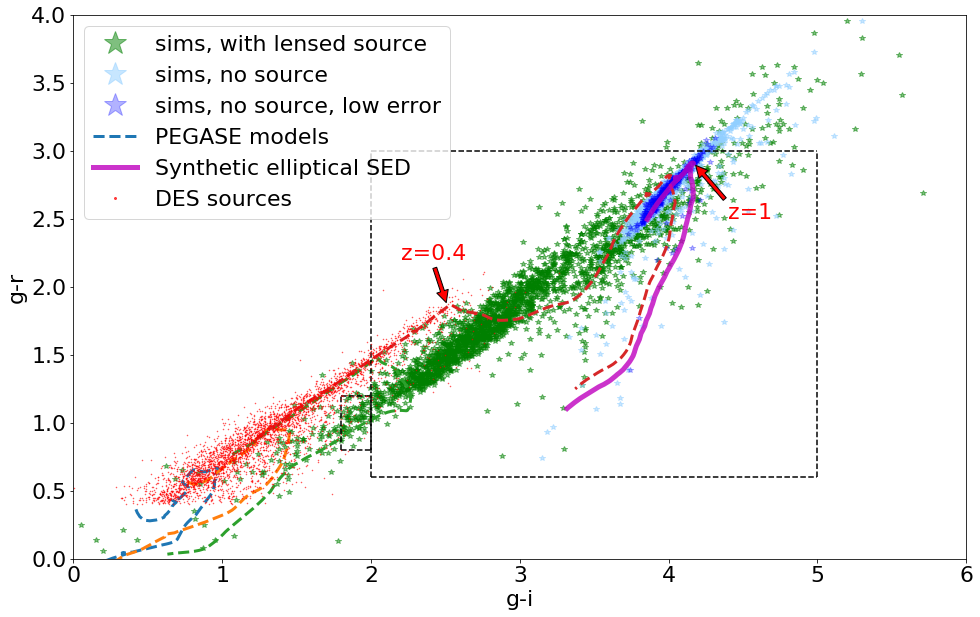
Figure 2: The colours (in $g-i$ and $g-r$ ) of simulated lenses at redshifts > 0.8, showing simulations without lensed source (blue/cyan) or with (green). As the simulated ellipticals are faint or undetectable in g by design, there are large errors in the measured $g$-band magnitudes; this diagonal scatter (i.e. along the g axis) is visible in the figure, compared to the raw colours of our LensPop synthetic 10 Gyr SED (redshifts 0.8-1.5 depicted in magenta). Simulated lenses with photometric g-band magnitude errors $<0.2$ are depicted in dark blue, the rest in cyan. We depict a set of red through blue PEGASE.2 (Fioc & Rocca-Volmerange, 1999) template tracks, with progressively increasing amounts of recent star formation to illustrate where normal z<1.5 unlensed galaxies are expected to lie. The red dashed line is the PEGASE 10 Gyr simple stellar population model (similar to our synthetic SED); the arrows point out kinks in the colour track at redshifts 0.4 and 1. A random selection of DES catalogue sources is depicted as red points, indicating where the denser parts of the catalogue lie; our colour cuts are depicted as black boxes.

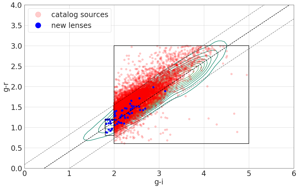
Figure 3: Catalogue sources (green) and new lens candidates (blue). Green contours indicated where simulated strong lenses lie. The dashed lines show a best fit colour-colour relation for the simulated lenses, with 3-sigma lines shown. We choose sources from the catalogue that are within the boxes depicted, where $2<g-i<5$, $0.6<g-r<3$, and where $1.8<g-i<2$, $0.8<g-r<1.2$.

3.2 Generating simulations

In order to optimise a neural network with millions of trainable parameters (“weights”) we require a training set of sufficient size. State-of-the art neural networks used in general computer vision applications require of order $10^{6}$ training examples for robust training (e.g. Krizhevsky et al., 2012). Given that the number of discovered lenses across all surveys and instruments is in the hundreds, we must simulate lenses in order to create a training set of sufficient size. We use a modified version of the LensPop code described in Collett (2015) for this purpose.

LensPop generates a population of synthetic galaxies with a singular isothermal ellipsoid (SIE) mass profile and redshifts, masses and ellipticities drawn from realistic distributions following the LensPop methodology (Collett, 2015). Deflector masses are drawn from the velocity dispersion function of SDSS (Choi et al., 2007) without redshift dependence and a constant comoving density out to redshift 2. Lens colours assume a 10Gyr-old quiescent SED. Sources are elliptical exponential disks with redshifts sizes and colours drawn from the COSMOS sample (Ilbert et al., 2009). Lens light is added to the resulting image using the fundamental plane relation (Hyde & Bernardi, 2009) assuming a de Vaucolours profile and the spectral energy distribution of an old, passive galaxy. We shift the brightness profile of the sources by one magnitude brighter in all bands to create a larger sample of detectable lenses. This makes the process more efficient in terms of detectable lenses generated per second; generating an unrealistically rich sample of bright, detectable lenses is not problematic when our goal is simply to train our CNN and not constrain lensing statistics in the real universe.

The LensPop code generates our synthetic population of lenses and sources. The simulations are then pruned as follows. Firstly, lenses with redshifts $>2$ and $<0.8$ are discarded. Lens images are then simulated using GRAVLENS (Keeton, 2001) raytracing code. Images in $g$, $r$, and $i$ bands are produced with seeing drawn from the DES Year 1 science verification data with a floor of $.9\arcsec$ in all bands; typical seeing of 1.1 - 1.2 $\arcsec$.

Simulated shot noise is added. Lenses with signal-to-noise $<3$, Einstein radii $<$ twice seeing and magnifications less than 3 are discarded as they are unlikely to be detectable in DES imaging. We generate two sets of images, as FITS files 100 pixels ($30\arcsec$) on a side, the first with both the flux from the lensed source - positive examples (“a strong lens”) and secondly, without - negative examples (“no lensing depicted”). These simulated lenses are combined with randomly chosen tiles from the DES imaging, to add sky and read noise, stars, realistic background and foreground objects, artifacts, etc. We assembled a training set of 250,000 images as depicted in Figure 4. A histogram of the redshifts of the simulations is depicted in Figure 5.

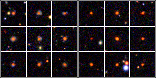
Figure 4: Simulated lenses for the training set (RGB images from $g$, $r$, $i$ bands). Left: With lensed source. Right: Without lensed source (negative examples).

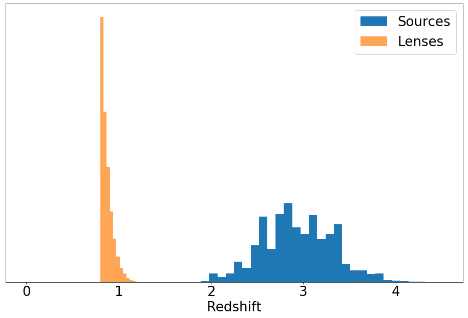
Figure 5: Redshift distribution of lens galaxies and lensed sources for simulations used in training the networks. This includes only lenses at redshift > 0.8 and the associated sources.

3.3 Training Convolutional Neural Networks

The convolutional neural networks were architected with four convolutional layers with kernel sizes 11, 5, 3 and 3 respectively, and one fully connected layer of 1024 neurons. The nonlinearity function is the rectified linear unit (ReLU); a dropout (see Hinton et al., 2012) of 0.25 is added after the last convolutional layer, and 0.5 between fully connected layers. This network architecture is similar to industry standard network architectures such as AlexNet (Krizhevsky et al., 2012), but much simpler than the most complex networks used for computer vision (e.g. ResNet (He et al., 2016), up to 1000 layers). The network contains a total of 8,833,794 trainable weights. The number of layers and their dimensions are free parameters, and an optimal architecture is still a matter of some guesswork. This network architecture was chosen based on previous experience (Jacobs et al., 2017), and was deemed fit-for-purpose based on the high accuracy realised during the training process. A deeper network could potentially result in higher training accuracy, however the practical limitation appears to be the translation from simulations to real sources see 5.4. A similar network to the one presented here was used by the authors to enter the Bologna Lens Finding Challenge (Metcalf et al., 2018) and placed third in the detection of simulated lenses in multiband imaging.

The networks were implemented, trained and run using code employing the Keras deep learning library and Theano numerical library (Team et al., 2016). Figure 6 depicts the network architecture; the description of the Keras model is also included as an appendix.

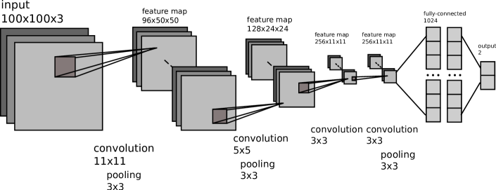
Figure 6: Architecture of neural networks used: Four convolutional layers with kernel sizes 11, 5, 3, and 3, and two fully-connected layers of 1024 neurons each.

In total, 20 CNNs with these dimensions are trained, with differences as outlined below. We create two training sets, as summarised in Table 1. Training set 1 consists of 125,000 simulated lenses and the same number of non-lensing elliptical galaxies. Training set 2 consists of 80,000 simulated lenses and 80,000 postage stamps of sources chosen at random from our search catalogue section 4.2 as negative examples. With the first training set, we ensure the network learns to reject simulations that do not exhibit detectable strong lensing, forcing it to learn from the morphology of lensing and not merely a characteristic of our simulations that inadvertently distinguishes the simulations from real galaxies. With the second training set, the networks will learn that objects we have not simulated - spirals, mergers, stars, an so on - are to be considered non-lenses. Since we expect only of order one lens in $10^{4}$ sources, this negative training set may be ‘contaminated’ by a few actual lenses, but this will not have a discernible impact on training since the contribution of each training example to the weight updates is equal.

The use of two training sets with different non-lens images, as opposed to a single larger training set combining both, has the advantage that we can tune the weighting given to the contribution of the two training sets when assembling a candidate set by choosing different score thresholds for the two networks. This gives more fine-grained control in exploring the trade-off between purity and completeness and tuning the size of the candidate set to examine.

Table 1: Training sets used to train neural networks.

Training set	Pos. examples	Neg. examples	Size
TS1	simulations	simulations	250,000
TS2	simulations	real galaxies	160,000

For each of these two training sets, we divide each into 10 equally-sized subsets (folds). For each fold, we train a network reserving that fold of the data as a validation set - not used for training, but used to measure training progress - and the remainder as the training examples. We thus obtain 10 networks trained on different subsets of the training examples to hand. This process is known as k-fold cross-validation (see Refaeilzadeh et al., 2009, for a detailed description). There is some stochasticity in the training process; the initial weights are randomised, the order in which the training set is fed to the network is also random, and by using slightly different training sets, each network thus trained will score candidates slightly differently. Using an ensemble allows us to smooth out the effects of outlier scores; we use the mean score from the 10 trained networks in selecting candidates. More than 10 networks per ensemble are unlikely to add additional information, but require GPU time to train. It has been shown (Hansen & Salamon, 1990; Krogh & Vedelsby, 1995) that using an ensemble of neural networks in this way can provide a significant boost to the accuracy of the system, e.g. a 2% increase in classification accuracy over the best performing network by an ensemble (Ju et al., 2017) - particularly if the networks are trained with different training data (Giacinto & Roli, 2001).

The networks are trained on FITS data in three bands ($g,r,i$), passed to the networks as 32-bit floating point values. The FITS data, which is background-subtracted, is further normalised so that across the training set, the mean value is zero and 99.7% of the values lie between -2.5 and 2.5. This is shown to optimise convergence by the training algorithm (LeCun et al., 1998).

We train the networks until further iterations no longer decrease the loss value on the validation set. At each epoch (iteration through the training set), we test the accuracy of the network on the training and validation sets, and calculate the loss for each. We halt training when the loss on the validation set has decreased by less than a parameter $\epsilon=0.0001$ for six epochs. Further training beyond this point is likely to lead to over-fitting to the training set.

3.4 Scoring and sorting candidate sources

Our target data set for the lens search is Dark Energy Survey (DES; Diehl et al., 2014; Flaugher et al., 2015; Diehl et al., 2016) Year 3 coadd images (Abbott et al., 2018; Morganson et al., 2018). This imaging consists of 10,346 tiles over 5,000 square degrees of sky. The number of epochs is ~4-6 per coadd object per band, with a limiting magnitude in $r$ of 24.9 and a pixel scale of $0.263\arcsec$/pixel. The mean seeing is $1.06\arcsec$ in $g$ (Diehl et al., 2018). We generate postage stamps in $g$, $r$, $i$ and bands of dimensions 100x100 pixels for each of the million sources in our target catalogue. Each of the postage stamps is scored using the pre-trained CNNs, to produce two scores in the interval (0, 1) corresponding to the two different training sets. We then examine the distribution of scores, and choose thresholds for each score to produce a subset of our catalogue for visual examination by human experts. We choose the threshold such that the candidate set is of a size that can be examined in a few hours, i.e. a few thousand images. RGB images of each source are examined by eye (by authors CJ, KG and TC) and graded using software, LensRater, developed for this purpose. We rate the candidates as 0) unlikely to contain a lens, 1) possibly containing a lens, 2) probably containing a lens and 3) almost certainly containing a lens. We then take the mean grade and assemble our final candidate catalogue from those graded 2 and above. In this paper we define false positives as any candidates that we judge to be below grade 1. We then estimate the completeness of our sample of lens candidates.

3.5 Estimating photometric redshifts

The objects we discover in our search are lens candidates. In the absence of spectroscopic follow up, we cannot know how many of them are genuine strong lenses, and of those that are, how many are in our target redshift range. In order to make a first-order approximation regarding the second question, we calculate photometric redshifts of the lens galaxies. We use the BPZ (Bayesian Photometric Redshifts) photo-z package. As inputs to the photo-z code we use colours measured from the DES Y3 coadd images in $griz$ with apertures fit manually to the galaxies (excluding blue source flux), with mag errors taken from the DES catalogue. We quote the best-fit and $2\sigma$ uncertainties output by BPZ.

3.6 Estimating the completeness of the sample

Our workflow involves the evaluation of machine-selected candidates by human astronomers for follow-up. The optimal sample would therefore include all sources that a human astronomer would grade as probable or definite lenses, and not those that would be graded otherwise, whether or not they are, in reality, strong lenses. The completeness of our sample, as a measure of what can realistically be detected in the imaging we are searching, is a function of what an astronomer can discern with confidence from a composite RGB image used for evaluation.

Collett (2015) used simulations to estimate the number of strong lenses discoverable in DES coadd imaging. Simulating the survey sky, using detectabity criteria of signal-to-noise in $g$ greater than 20, magnification greater than 3, and an Einstein radius greater than the seeing (~$1\arcsec$), Collett predicts ~1300 lenses should be discoverable by inspection of the images. These detectable lenses had a mean lens redshift of 0.42; 8% (~110) were at redshift 0.8 to 2.

How many of these theoretically-detectable lenses would actually be selected as good candidates by a human astronomer following our lens-finding pipeline is a testable question. To better understand this threshold, we collect one further piece of data. We assembled a set of 5000 postage stamps containing 2500 real galaxies, 1000 simulated lenses, 1000 simulated ellipticals and 500 simulated ellipticals with unlensed blue sources nearby (“phonies”) and presented these, blinded, to authors TC and KG to evaluate. We then examine the number of simulated high-redshift lenses graded highly by the inspectors. Measuring the fraction of simulated lenses that were rated highly assists us in making an estimate of the true number of lenses we can expect to find in the survey using our automated pipeline. Of high-redshift simulated lenses examined, 51% were given grade 0, indicating that estimates of detectability are highly dependent on image quality and grading methodology, and can easily be overestimated. We discuss this further in section 5.3.

4 Results

4.1 Training neural networks

Two ensembles of neural networks were trained as described in section 3.3. For the first ensemble, trained on simulated lenses with and without lensed sources, the training converged after $30\pm 1$ epochs in each case. The accuracy (the fraction of a sample classified correctly: true positives + true negatives a divided by number of items tested) on the respective validation sets of the 10 networks in the ensemble was $98.6\pm 0.1\%$. The training progress for a single network is depicted in Figure 7; after a single epoch, the training accuracy was 87%, converging slowly on the final value. On the second training set, composed of simulated lenses and random sources from the catalogue, training converged in fewer epochs, $20\pm 2$, with a validation accuracy of $99.4\pm 0.1\%$.

In Figure 8 we depict the Receiver Operating Characteristic curve for the first network, trained on simulated lenses and non-lenses, when evaluated on examples not used during training. This figure depicts the trade-off between the true positive rate and the false positive rate achieved for different values of the score threshold. A perfect system would include the point at (0, 1), namely zero false positives and all true positives, and have an area under the curve (AUC) of 1. The AUC is for the first network is 0.9993; for the second, it is 0.9998, and so the curve is not shown.

The total training time was approximately 40 hours for the first ensemble and 24 hours for the second, trained on an NVidia K80 GPU and Intel Xeon E5-2698 cpu with 12GB RAM and a batch size of 128 images.

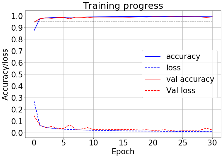
Figure 7: Training of a neural network, demonstrating convergence on high accuracy and low loss. The dashed lines show the value of loss function, evaluated over the image set, and the solid line the classification accuracy. Blue: Loss/accuracy on the training set. Red: Loss/accuracy on validation set of images not used for training. The curves for other networks are similar and so are not shown.

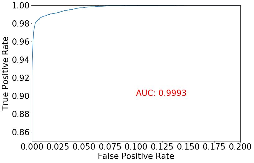
Figure 8: Receiver Operating Characteristic curve for the CNN trained on training set 1, consisting of simulated strong lenses and simulated elliptical galaxies without visible lensing. This curve shows the trade off between a desired true positive rate and the number of false positives produced by the network for different values of the score threshold. The area under the curve (AUC) for this network is 0.9993. For training set 2, the AUC is 0.9998, so the curve is not shown.

4.2 Scoring catalogue sources and selecting a candidate set

Scoring a batch of 128 100x100 pixel FITS images in three bands took ~3ms. With the overheads of loading the files into memory, and scoring with 20 networks, scoring the 1 million sources in our catalogue took approximately six hours. The 254GB of images were stored in HDF5 databases in 15GB chunks and the CNNs were able to load the images in batches using the HDF5 files directly, a faster process than working with 1 million or more individual files.

We scored each of the 1.1 million postage stamps with all of the 10 trained networks in each of the two ensembles. We took the mean score from each ensemble to produce two scores for each image. Of the 1,061,868 sources scored by the first ensemble of networks, 576,025 (54%) were scored less than 0.01; and by the second ensemble 967,348 (91%). The first ensemble scored 35,332 sources above 0.99; the second, only 433. The scores are summarised in Table 2 and a histogram depicting the distribution of scores is presented in Figure 9.

Table 2: Distribution of CNN scores for the two ensembles.

Score	Ensemble 1	Ensemble 2
< 0.01	576,025	967,348
> 0.5	156,776	9328
> 0.99	35,332	433
> 0.999	10,847	97

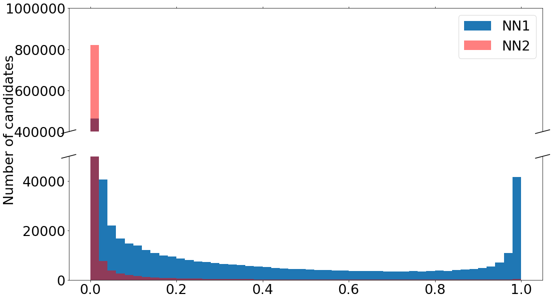
Figure 9: Distribution of scores of sources scored by CNNs. For the first ensemble, of 1.1 million sources, 3144 had a score of 1.0 (definitely a lens), 668408 had a score < 0.01. For the second, there were no perfect 1.0 scores, and 810,604 scored < 0.01. There are 358 sources in the final bin with score > 0.98.

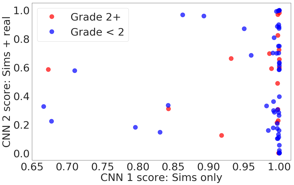
Figure 10: Scores received from the CNNs by the most highly-graded lens candidates. Red: Graded 2-3 ("probably" or "definitely" lenses). Blue: Scores below 2 (possibly" lenses). Some of the best candidates were scored as low as 0.2 by the network trained on simulations and real galaxies.

Due to the subtleties of lensing morphology in this redshift range, and the large number of sources evaluated, false positives are a concern. We wish to produce a candidate set for visual inspection that is as small (pure) as possible while containing the majority of the detectable strong lenses in the survey (high completeness). As the discoverable lenses are not known a priori, evaluating completeness is only possible in approximation and after evaluation by eye has been completed (see section 5 below).

We choose candidates for visual inspection by selecting score thresholds and examining candidates that scored higher than this number by the networks. The thresholds $t_{1}$ and $t_{2}$ are free parameters; the scores $s_{1}$ and $s_{2}$ are output by the two CNN networks for each source tested. We examine candidates where, for that source, $s_{1}>t_{1}$ and $s_{2}>t_{2}$. This filters many sources scored highly by one network but not the other.

We examine candidate sets as per Table 3. With thresholds (0.65, 0.1) we obtain 3,582 images to examine; with threshold (.9999, 0) a further 1,841 candidates; and in the area of the extended catalogue, 1,878 images with thresholds (0.95, 0.55) for a total of 7,301 images. We choose these candidate sets so as to explore the relative contribution of the two CNN ensembles while returning a manageable number of candidates. Following inspection of these candidates, author CJ examines a further 9,428 candidates with scores above thresholds (0.999, 0) for a total of 16,729 images. The set with scores (0, .999) contained only 49 images, all false positives.

4.3 Examining candidate lenses

Of 16,729 the candidates examined, 250 had a grade > 0, 87 $\geq 1$ and $29\geq 2$. With grade 0 candidates, we have an overall false positive rate (false positives = highly scored non-lenses) of 98.5% amongst the candidates we reviewed. Of the candidate sets we reviewed, the purest was the 3,582 candidates with scores $s_{1}>0.65$ and $s_{2}>0.1$, which yielded 43 candidates with grades > 1 for all examiners. Overall time taken to examine candidates is approximately five hours of astronomer time. Of the 87 candidates identified with scores $\geq 1$, 4 are known from a previous search (Diehl et al., 2017).

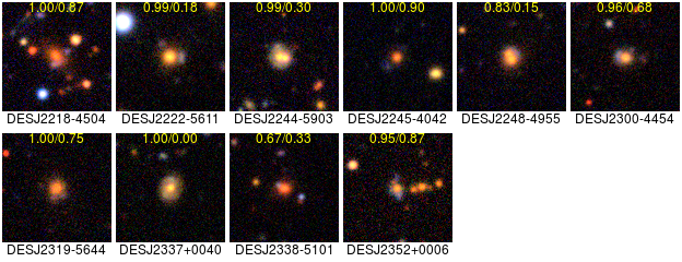
Figure 13: 58 new lens candidates, with a grade $1\geq\text{grade}>2$, discovered in DES imaging data using CNNs. The CNN scores are shown in yellow text. The candidates are described in Table LABEL:tbl:new_candidates.

The lenses with a grade $\geq 2$ are presented in Figure 11 and those with $1\geq\text{grade}<2$ are shown in Figure 13. The candidates are summarised in Table LABEL:tbl:new_candidates, including with the photometric redshifts for the lenses with $2\sigma$ errors estimated by BPZ.

The scores the candidate lenses received from the networks are presented in Figure 10. Most candidates received scores of approximately 1.0 from the CNN trained on simulations, but were more evenly distributed in their scores from the second CNN trained on simulations and real galaxies. There is no significant difference in CNN scores by grade of lens candidate. The mean scores for candidates of grade 2+ were .97 and .39 for the two networks; for grade $<2$, the mean scores were .87 and .42 respectively.

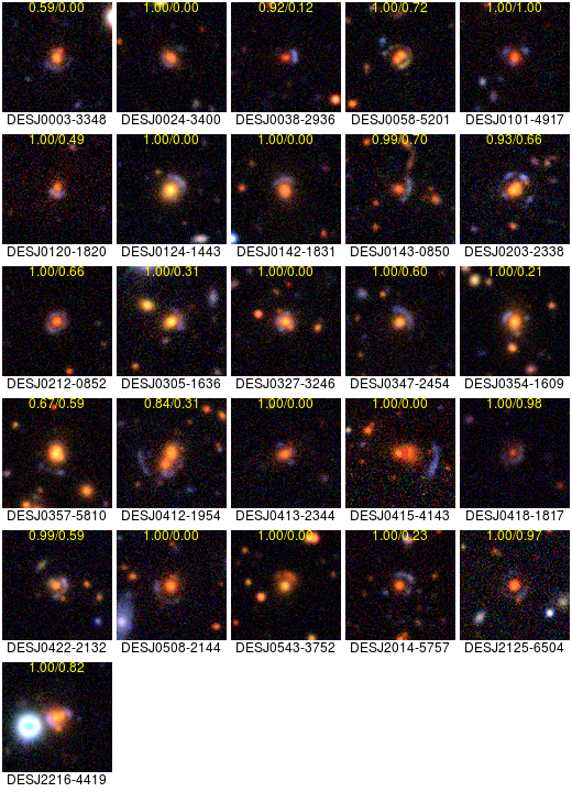
Figure 11: 26 new lens candidates, with a grade $\geq 2$, discovered in DES imaging data using CNNs. The scores from the two CNNs are shown in yellow text. The candidates are described in Table LABEL:tbl:new_candidates.

Table 3: Summary of candidate sets examined. These candidate sets were selected by the neural networks with scores greater than the thresholds $t_{1}$ and $t_{2}$ and examined by the authors. New candidates indicates candidates that are unique to that search; search 4 contained 22 candidates, but only four that were not found in the other searches, demonstrating the rapidly diminishing returns. Searches 1, 2, and 4 were applied to the larger source catalogue, search 3 was applied to the extended catalogue only, as described in section section 3.1

.

Search	size	$t_{1}$	$t_{2}$	candidates >= 2	New candidates	Purity
Search 1	3582	0.65	0.1	11	43	1.2%
Search 2	1841	0.9999	0.0	5	15	0.8%
Search 3	1878	0.95	0.55	6	21	1.1%
Search 4	9428	0.999	0.0	3	4	0.04%

Our catalogue was selected by examining the combined lens and source colours of simulated lenses (section 3.1). Figure 3 depicts the position in g - r and g - i colour space of the new lens candidates, as well as the simulations and sources from our search catalogue.

We include one candidate, DESJ0003-3348, discovered serendipitously in the control sample inspected in section 3.6. It received scores of .59 and 0.00 from the two networks respectively.

5 Discussion

5.1 Efficiency of the method

Convolutional Neural Networks have proven themselves in a variety of computer vision problems both broadly and within astronomy, including in other lens finding applications. Here we also find that they performed well on a more targeted lens search, producing dozens of high quality candidates with a few hours of astronomer inspection time. Inspecting the lenses with LensRater (section 3.4), we find that examining 3000 candidate images per hour is a sustainable rate. We examined approximately 7300 postage stamps, or 2.5 hours, in selecting the catalogue of new lens candidates presented in section 4. Thus, assuming all candidates are genuine lenses, we discover ~30 genuine lenses in our redshift range per hour of astronomer time and achieve completeness close to 100% (see below) in a few hours. In comparison, examining the entire catalogue of 1 million lenses would take over 13 days at this rate, and 11 years for all sources in the survey.

We can almost certainly increase the completeness of our catalogue by examining more potential candidates. However, as we reduce the neural network score threshold to examine, the size of the candidate set increases exponentially, as does the time investment required for each additional candidate. As the candidates become less obvious to the human eye (fainter, arc-like features more subtle), so does the number of false positives increase. We examined 7,301 candidates and identified 83 probable or definite lenses (four of which are previously known). Examining a further 9,428 candidates uncovered only four more credible lenses in addition to those already identified. We conclude that these diminishing returns indicate our sample is relatively complete at this point.

5.2 Catalogue selection

We restrict our search to postage stamps of a subset of sources in the DES survey catalogue. The catalogue cuts, in $g-i$ and $g-r$ colour space (section 3.1), were chosen by reference to the integrated colours of our simulated strong lenses in the desired redshift range. Figure 3 depicts the locations of both the simulations and the new lens candidates in this space. We find good agreement between the new candidates and the colours predicted by the simulations. The candidates we present are significantly closer to the area in the space where the simulations reside as opposed to the catalogue sources more generally which exhibit greater scatter. Searching a smaller catalogue that conformed more closely to the contours of the simulated lenses would therefore seem like a promising avenue to yield a purer sample without sacrificing completeness. Of our total catalogue of 1.1 million sources, 36% lie $>3\sigma$ from the line best fit to the lenses. Although the CNNs perform some of this pruning for us (of our candidate sets examined, 85% lie within this region), some time saving is achievable here. Of the candidates in our catalogue, all lie within the $3\sigma$ limit.

The density of lens candidates increases towards the bluer end of the cuts we made in both colour dimensions. This suggests widening our search may yield further candidates. However, this area of the colour space contains a much greater density of catalogue sources; for instance, while a million sources exist in the range we chose, an additional 2.5 million sources are present if we go .5 mag bluer, and 10 million sources at 1 mag bluer in each axis. Thus, assuming a constant rate for false positives, we would expect our purity to drop by a factor of 2.5 - 10, yielding rapidly diminishing returns. The density of simulated lenses was lower in this part of colour space; 91% of simulations are in the original catalogue area, and 5% in the supplementary catalogue. Blueward of the catalogues we searched, many spiral galaxies are to be found, and we expect that a higher false positive rate would accelerate the diminishing returns in extending the search in this direction.

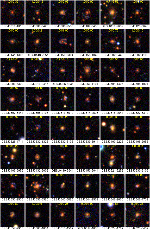
Figure 12:

5.3 Completeness of the candidate sample

In Jacobs et al (2017) we used CNNs to search CFHTLS, which had been the subject of several fruitful lens searches previously, including visual inspection of the entire survey area ($171\text{deg}^{2}$) by citizen scientists. Using a catalogue of lenses discovered in previous searches, we were able to estimate a completeness of 21-28% in a candidate set of 2465 sources. Estimating completeness of our current sample is more difficult as we have no pre-existing reference sample of high-redshift lenses in the survey footprint against which to compare, and must rely on simulations to estimate the number of discoverable lenses.

The number of detectable lenses in a survey is a function of both the depth and seeing of the imaging, and the methodology used to examine sources. Collett (2015) modelled the number of detectable lenses in DES, and estimated up to 1300 could be found, of which 110 are in our target redshift range. This estimate assumes an optimal stacking strategy, and inspection of lens-subtracted images, which we were unable to perform due to difficulties in modelling the PSF of the coadd imaging.

We used LensRater, the candidate ranking pipeline described in section 3.6, to evaluate a mixture of simulated lenses, potentially confusing chance alignments, and real galaxies. For simulations at all redshifts, only 20% received a grade > 0 by a human inspector. Of 500 simulated high-redshift lenses in the sample with Einstein radii >  $2\arcsec$, 247 (49%), 99 (19.8%) and 24 (4.8%) received grades 1, 2, 3 respectively. Detectability is aided at higher redshifts as the effective radius and apparent luminosity of the lens are smaller, allowing for greater image separation between source and lens. The estimate of 130 lenses from (Collett, 2015) includes lenses with smaller Einstein radii (59% are smaller than $1.25\arcsec$), so this gives us an upper bound on the number of lenses we expect to find. 247 (49%) received a grade $\geq 0$, 99 (19.8%) received a grade $>1$, and 24 (4.8%) received a grade of $\geq 2$. Detectability is aided at higher redshifts as the effective radius and apparent luminosity of the lens are smaller, allowing for greater image separation between source and lens. The estimate of 130 lenses from (Collett, 2015) includes lenses with smaller Einstein radii (59% are smaller than $1.25\arcsec$), so this gives us an upper bound on the number of lenses we expect to find. We therefore conclude that in DES, of order a few tens of high-redshift lenses have the signal-to-noise and image separation required to be selected confidently by a human inspector. Our test on simulations can also give us some indication of the reliability of inspection grades. Of those with grade 3, 100% were simulated lenses; for grade 2, 98%; and for grade 1, 93%. Conversely, only 2% of the "phonies" received a grade > 0.

To estimate the completeness of our search we also need to know how many of the discovered lenses lie in the targeted redshift range. The reliability of the photometric redshifts is limited by the number of bands, contamination with flux from the blue lensed sources, and the Bayesian priors used by the code. Due to the comparative rarity of massive galaxies, the prior on the redshift distribution in BPZ strongly penalizes elliptical galaxies with i~18 being beyond z> ~0.8. However, since our galaxies are selected as strong lenses they must be massive and likely live in the bright tail of the luminosity function. We therefore expect that the BPZ prior is biasing the photometric redshifts low, but we have not quantified this effect. Of our sample of 84 candidates, 76 are within the targeted redshift range within the quoted $2\sigma$ errors, and 28 (33%) within $1\sigma$. From this, we conclude that a sizeable fraction of our candidate set are within the right redshift range, independently of whether they are in fact strong lenses.

Of the lens candidates presented in Diehl et al. (2017), a previous search of the DES imaging (see Section 5.6), 102 fall within out catalog. Of these, 33 are galaxy-scale lenses consistent with our grading scheme but were not detected in our CNN-based search. This may indicate that our completeness estimate is high. Another possible explanation is that the CNNs have correctly filtered for redshift. None of these 33 candidates have published photometric redshifts greater than 0.8, and only two have redshifts less than two times the stated redshift error below 0.8.

Here we present a catalogue of 84 candidate lenses; 26 have a grade $\geq 2$. Based on the above, we expect that the majority of our sample will be confirmed as lenses, but spectroscopic followup will be required to constrain the fraction that are in the correct redshift range. Based on the photometric redshifts, we expect a at least few tens of candidates to be confirmed, which is of a similar order to the expected number of discoverable lenses. Although it is not possible to constrain the error on this estimate until follow-up is undertaken, the search seems likely to increase the number of known lenses at high redshift by a factor of a few.

If this result is confirmed, this also represents an improvement in purity and completeness over previous searches. Although there is still room to improve the method, we attribute the improved performance (compared to Jacobs et al. (2017)) to the use of CNN ensembles, improved training set simulations, and the targeted search, which constrains the morphological variety of the lenses sought, particularly in lens colour.

We note our candidates include one, DESJ0543-3752, with a red arc. This indicates that while the CNNs clearly make use of both colour and morphology, a clear signal in only one can still produce a high score.

5.4 False positives

After testing trained networks on simulated lens images, the neural networks are able to distinguish lenses from non-lenses with high accuracy. Selecting images with scores greater than 0.5 as lenses, the trained networks have accuracy between 98.6 and 99.4% (for networks 1 and 2 respectively). If this performance translated perfectly to the real survey imaging, we would expect that for 1 million sources examined, we would achieve a completeness of ~99% of the lenses in our catalogue - approximately 100 - and 10,000 false positives (a purity of 1%). Setting aside candidates that could be lenses but are of low quality (score 1), we examined 7,301 sources to find 52 lens candidates, a purity of 0.7%. By that measure, the CNN search results roughly reflect the performance expected from training. The majority of the sources in this candidate set can be immediately rejected by human astronomers. This implies a significant reduction in false positives ought to be possible. Since real-world performance now approximates the training performance, we conclude that investigating the use of deeper and more complex networks, as well as improving the simulations, may be warranted.

The false positives in the sample, i.e. sources we rate as very unlikely to be a lens/having no discernible features of strong lensing, exhibit a wide variety of morphologies, but we can identify a few clear trends:

• Blue near red: sources of plausible colours, but no obvious morphology that would suggest strong lensing (~10%);

• Low signal to noise: Faint sources with apparent blue flux but insufficient information present to clearly indicate lensing (~25%);

• Imposters: Blue spiral arms and other features that mimic lensing arcs (~5%);

• Unclear: Some irregular sources don’t resemble typical examples from either category, and so the CNNs’ best guesses are undefined (~60%).

A representative sample is depicted in Figure 14. In searches aimed at finding lenses at other redshift ranges, we find that spiral and ring galaxies form a large fraction of false positives, as (for instance) blue star-forming regions in the arcs of spiral arms can trigger the arc-detection features of the neural network strongly. In this search, although spirals are present in the false positives, they form a smaller fraction of the false positives we examined. Given the colours and morphology of lenses at the higher redshift range, we expect fewer spirals - morphological similarities notwithstanding - will activate the networks strongly enough to achieve a high probability score.

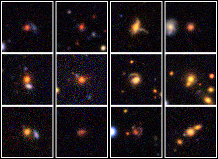
Figure 14: False positives amongst candidate lenses. Left: Blue near red objects. Second from left: Low signal to noise objects. Second from right: False arcs. Right: Objects with no clear confusing feature.

The false positives suggest two deficiencies in the training set. Firstly, there may be too many simulated lenses that while theoretically detectable, would not be graded highly on inspection by a human expert. Since such lenses, when detected in the survey imaging, make poor candidates for follow-up, we may wish to train networks instead to reject them. Secondly, we are training the networks to place all candidates in one of only two categories, lens or non-lens. Highly irregular objects, which do not resemble typical examples of either lensing or non-lensing objects, receive unpredictable scores. Despite their rarity, a future training set could include a greater proportion of irregular galaxies; however, by their nature it is uncertain how successful a CNN would be at learning features from these objects. Training the networks to place objects in more than two categories may improve the situation.

Internally, the neural networks create a highly non-linear decision boundary in the parameter space of all possible images, in this case 30,000 dimensions (100x100 pixels in three bands). Nguyen et al (2015) demonstrated that in traditional computer vision applications using deep neural networks, it is possible to construct images that appear to be white noise to a human observer but strongly activate the networks for a particular image category. This implies that if we examine enough noisy images, as we will with large surveys, we will encounter some which, despite their appearance to a human being, contain a configuration of values that activate a part of the network strongly indicative of one of the two or more defined categories. To enhance the purity of lensing searches in future surveys, we seek false positive rates of order 1 in 100,000 or better - an ongoing challenge when noisy images may activate by chance particular parts of a trained network that indicate lensing. Further use of ensembles of networks may mitigate this problem.

In the preceding discussion, we have considered false positives to be candidates that a human inspector deems unlikely to be a strong lens. However, some of these false positives are likely to be strong lenses, only of a sort a human inspector would not grade highly. It is possible that with improved inspection tools to aid the inspector, such as lens-subtracted images, a human would be better able to identify lenses that the networks score highly but are difficult to spot in the RGB images of the sort we use here.

5.5 Choosing a candidate set

All automated lens searching methods ultimately rely on visual inspection to confirm the quality of potential lens candidates. The neural networks provide a score representing a probability that a source is a strong lens. The output of a probability score by neural networks, if provably consistent and robust, is of some value in an astronomy context as it allows a more fine-grained allocation of follow-up resources than the course-grained and highly stochastic "yes-no-maybe" grades produced by human inspectors.

How to use this information to choose sources to examine is up to the user. Our methodology involved examining the size of candidate sets that satisfied various score criteria, and visually inspecting several of these of a manageable size (i.e. a few thousand). Beyond this size, the law of diminishing returns makes visual inspection less efficient as candidate sizes increase exponentially and the quality of candidates decreases. Without a reference sample of lenses, it is difficult to know what the optimal threshold for a candidate set is in terms of the trade-off in purity and completeness.

We train networks with two different training sets (simulated non-lenses, and real galaxies as non-lenses). We do this because real galaxies that do not match the parameters of the simulated ETGs have a high potential to confuse the network trained only on simulations; this follows, as the network will have never seen anything resembling (say) a spiral galaxy and thus its response to that morphology is undefined. Beyond this intuition, the contribution of the two neural network scores is a free parameter without real constraints. Inspection of candidate sets of a similar size from each network suggests comparable purity. To assist future searches, examining a much larger set of candidates, perhaps by citizen scientists, could assist in constraining the optimal settings.

In grading candidates, we discover many sources that could possibly be a lens, where flux from a potential lensed source could be discerned above the noise, and in a plausible configuration. However, these sources are neither bright enough nor distinct enough to the human eye to grade higher. These candidates, although not false positives in the usual sense, may not be of a quality that warrants the expensive spectroscopic follow-up required to do subsequent science. A future training set could include simulated lenses with low signal-to-noise as negative examples, to heighten the chance of activating on only the strongest and most interesting discoverable lenses.

We reject many candidates offered by the lens-finder with high scores due to insufficiently strong lensing features. However, we examine the candidates as RGB images; the neural networks operate directly on the calibrated FITS images and so are not as limited in dynamic range as the human eye. We cannot be certain that the CNN is seeing something that strongly indicates lensing that we cannot. This also suggests that improvements in the tools used by the human vetters, such as a range of contrast settings and single-band imaging or lens-subtracted images, may improve the grading process.

5.6 Comparison to other DES strong lens searches

Diehl et al (2017) conducted a search of the Dark Energy Survey science verification (SV) and Year 1 (Y1) observations and identified 374 candidate strong lens systems of which the authors designate 47 of high quality. The candidates were selected using several techniques including colour-based searches (“Blue Near Anything”) and searches of a known catalogue of massive Early-Type Galaxies. Assembling this candidate set required visual inspection of approximately 400,000 cutout images. Nord et al. (2016, 2018 in prep) searched DES SV and Y1 data for group and cluster-scale strong lenses, inspecting 250 square degrees of the SV and over 7000 catalogued clusters, identifying 53 lens candidates in the former and 46 in the latter, of which 21 were confirmed spectroscopically. While the comparison is complicated by the fact that our networks were trained specifically for lenses at high redshift, we were able to obtain high completeness after visual inspection of only ~17,000 candidate images (and only slightly less complete at 7,301). This suggests that our neural network-based algorithm is considerably more efficient (in terms of human inspection time if not in terms of GPU resources). This is consistent with the intuition that the morphological information learned by the CNNs (but absent in the colour-based search methods) contains information of high value in identifying strong lenses.

5.7 Future work

The method detailed in this work is readily applicable to lens searches at other redshifts and in other surveys. Improvements for future searches will include expanding the variety of galaxies represented in training sets, realistic variations in seeing in simulations, and simulating lenses using models fit to real potential lens galaxies. The number and architecture of the neural networks trained are still free parameters. As more lenses are discovered in the survey these parameters may be more easily constrained.

In this paper we have estimated completeness against lenses a human expert can confirm through visual inspection. Understanding the detectability criterion better may enable the development of improved inspection tools or mechanisms such as displaying lens-subtracted images. If the human thresholds are understood better training sets, that exclude real strong lenses that fall below this threshold, will produce more useful candidate sets. Future work will use simulations to better constrain the lensing parameters that best facilitate human certainty.

Realising the scientific potential of this catalogue will require confirmation of the lenses, and the measurement of lens and source redshifts. Higher-resolution imaging could also confirm lenses. With improved seeing at or below $.6\arcsec$, a robust measurement of the Einstein radius would be possible, sufficient for mean total density profile slope measurement using the method employed by Sonnenfeld (2013) and others.

6 Conclusion

Here we present a catalogue of 84 new high-quality strong lens candidates from the Dark Energy Survey Year 3 coadd imaging. For our target population of lenses at redshift $>0.8$ in DES coadd images, we estimate this sample to include the majority of those detectable in this imaging, pending follow up spectroscopy to confirm our candidates. If confirmation is forthcoming, this will increase the sample of strong lenses at these distances by a factor of 3-5. To achieve this across the 5000 square degrees of the DES footprint required only four to five hours of candidate inspection time by lens experts.

In recent years, convolutional neural networks have proven a promising technique in lens-finding and other astronomical classification applications. Some tens of new candidate strong lenses have been identified using deep learning already. With thousands or tens of thousands waiting to be discovered in upcoming surveys, further development of this method remains a promising area of research.

Here we apply convolutional neural networks to a search targeting lenses at redshifts $>0.8$. The search is motivated by the small sample of lenses known at these distances ($<10$) and the strong potential for a confirmed sample to impact our understanding of the formation histories of elliptical galaxies at early times, in particular by helping to constrain the evolution of the total density slope with redshift. At the targeted redshift range, the lenses have a particular morphology, where the central deflector is very faint in $g$ band, which may be learned by the ANNs during training and reduce the number of false positives.

This method, and the pipeline developed in this work, can be readily adapted to other surveys. Adjusting simulations to match the filters, seeing and resolution of the target survey is likely necessary to achieve good results. Future work will focus on increasing the purity of samples further by discarding a greater proportion of false positive or sub-optimal candidates. Our simulations can be improved, with more realistic variations in colour and morphology (e.g. groups, mergers, or spiral galaxies) possible. The simulated seeing values were drawn from DES Y1 Science Verification values, and was not matched to the DES Y3 coadd tiles used to construct the simulations. This should be eliminated as a possible source of error. Trained networks could also be improved with online learning using the information gained by inspecting candidates; this would complement e.g. citizen science initiatives, with human volunteers helping networks re-train by learning from false positives labelled by expert inspection.

Acknowledgements: This paper has gone through internal review by the DES collaboration.

This research was supported by the Australian Research Council Centre of Excellence for All Sky Astrophysics in 3 Dimensions (ASTRO 3D), through project number CE170100013.

TEC is supported by a Dennis Sciama Fellowship from the University of Portsmouth.

Funding for the DES Projects has been provided by the U.S. Department of Energy, the U.S. National Science Foundation, the Ministry of Science and Education of Spain, the Science and Technology Facilities Council of the United Kingdom, the Higher Education Funding Council for England, the National Center for Supercomputing Applications at the University of Illinois at Urbana-Champaign, the Kavli Institute of Cosmological Physics at the University of Chicago, the Center for Cosmology and Astro-Particle Physics at the Ohio State University, the Mitchell Institute for Fundamental Physics and Astronomy at Texas A&M University, Financiadora de Estudos e Projetos, Fundação Carlos Chagas Filho de Amparo à Pesquisa do Estado do Rio de Janeiro, Conselho Nacional de Desenvolvimento Científico e Tecnológico and the Ministério da Ciência, Tecnologia e Inovação, the Deutsche Forschungsgemeinschaft and the Collaborating Institutions in the Dark Energy Survey.

The Collaborating Institutions are Argonne National Laboratory, the University of California at Santa Cruz, the University of Cambridge, Centro de Investigaciones Energéticas, Medioambientales y Tecnológicas-Madrid, the University of Chicago, University College London, the DES-Brazil Consortium, the University of Edinburgh, the Eidgenössische Technische Hochschule (ETH) Zürich, Fermi National Accelerator Laboratory, the University of Illinois at Urbana-Champaign, the Institut de Ciències de l’Espai (IEEC/CSIC), the Institut de Física d’Altes Energies, Lawrence Berkeley National Laboratory, the Ludwig-Maximilians Universität München and the associated Excellence Cluster Universe, the University of Michigan, the National Optical Astronomy Observatory, the University of Nottingham, The Ohio State University, the University of Pennsylvania, the University of Portsmouth, SLAC National Accelerator Laboratory, Stanford University, the University of Sussex, Texas A&M University, and the OzDES Membership Consortium.

Based in part on observations at Cerro Tololo Inter-American Observatory, National Optical Astronomy Observatory, which is operated by the Association of Universities for Research in Astronomy (AURA) under a cooperative agreement with the National Science Foundation.

The DES data management system is supported by the National Science Foundation under Grant Numbers AST-1138766 and AST-1536171. The DES participants from Spanish institutions are partially supported by MINECO under grants AYA2015-71825, ESP2015-66861, FPA2015-68048, SEV-2016-0588, SEV-2016-0597, and MDM-2015-0509, some of which include ERDF funds from the European Union. IFAE is partially funded by the CERCA program of the Generalitat de Catalunya. Research leading to these results has received funding from the European Research Council under the European Union’s Seventh Framework Program (FP7/2007-2013) including ERC grant agreements 240672, 291329, and 306478. We acknowledge support from the Australian Research Council Centre of Excellence for All-sky Astrophysics (CAASTRO), through project number CE110001020, and the Brazilian Instituto Nacional de Ciência e Tecnologia (INCT) e-Universe (CNPq grant 465376/2014-2).

This manuscript has been authored by Fermi Research Alliance, LLC under Contract No. DE-AC02-07CH11359 with the U.S. Department of Energy, Office of Science, Office of High Energy Physics. The United States Government retains and the publisher, by accepting the article for publication, acknowledges that the United States Government retains a non-exclusive, paid-up, irrevocable, world-wide license to publish or reproduce the published form of this manuscript, or allow others to do so, for United States Government purposes.

Table 4: New candidates from visual inspection of the neural network-selected sources, sorted by grade.

Candidate	object id	RA	dec	grade	imag	$z_{phot}$
DESJ0003-3348	139823797	0.8183	-33.8012	3.00	19.77	0.56 $\pm$ 0.31
DESJ0347-2454	378100572	56.9356	-24.9087	3.00	19.77	0.51 $\pm$ 0.30
DESJ0203-2338	67920213	30.7667	-23.6340	3.00	19.15	0.58 $\pm$ 0.31
DESJ2216-4419	76102671	334.1592	-44.3222	3.00	19.05	0.53 $\pm$ 0.30
DESJ2014-5757	166130477	303.5808	-57.9504	2.67	20.64	0.76 $\pm$ 0.34
DESJ0143-0850	266637953	25.8622	-8.8392	2.67	20.48	0.58 $\pm$ 0.31
DESJ0142-1831	266036534	25.7203	-18.5211	2.67	19.62	0.57 $\pm$ 0.31
DESJ0124-1443	223066247	21.2211	-14.7174	2.67	18.88	0.44 $\pm$ 0.36
DESJ0543-3752	443873820	85.7586	-37.8770	2.67	20.06	0.54 $\pm$ 0.30
DESJ0415-4143	402556256	63.9363	-41.7295	2.33	18.92	0.75 $\pm$ 0.34
DESJ0101-4917	290048397	15.4918	-49.2939	2.33	20.31	0.68 $\pm$ 0.33
DESJ0357-5810	482065451	59.4035	-58.1815	2.33	18.69	0.53 $\pm$ 0.30
DESJ0354-1609	386476783	58.5761	-16.1645	2.33	19.34	0.53 $\pm$ 0.30
DESJ0212-0852	90442652	33.1051	-8.8697	2.33	20.23	0.59 $\pm$ 0.31
DESJ0038-2936	157799078	9.6926	-29.6019	2.33	21.13	0.71 $\pm$ 0.34
DESJ0058-5201	283879328	14.6447	-52.0332	2.33	19.67	0.59 $\pm$ 0.31
DESJ0120-1820	354176405	20.1074	-18.3338	2.33	20.77	0.71 $\pm$ 0.34
DESJ0305-1636	337847674	46.3197	-16.6037	2.00	19.30	0.51 $\pm$ 0.30
DESJ2125-6504	191159999	321.3001	-65.0741	2.00	19.88	0.73 $\pm$ 0.34
DESJ0024-3400	204184446	6.2373	-34.0148	2.00	20.01	0.58 $\pm$ 0.31
DESJ0422-2132	496451011	65.5759	-21.5461	2.00	20.23	0.54 $\pm$ 0.30
DESJ0327-3246	361760653	51.7973	-32.7762	2.00	19.55	0.52 $\pm$ 0.30
DESJ0413-2344	400295190	63.4213	-23.7395	2.00	20.17	0.58 $\pm$ 0.31
DESJ0412-1954	401080425	63.1615	-19.9023	2.00	19.07	0.57 $\pm$ 0.31
DESJ0418-1817	405038616	64.6387	-18.2982	2.00	22.13	0.86 $\pm$ 0.36
DESJ0508-2144	413900270	77.2053	-21.7419	2.00	19.58	0.65 $\pm$ 0.32
DESJ2300-4454	106547800	345.0133	-44.9065	1.67	20.01	0.51 $\pm$ 0.34
DESJ0546-2000	445925268	86.5211	-20.0071	1.67	19.18	0.53 $\pm$ 0.30
DESJ2218-4504	75469120	334.7402	-45.0738	1.67	19.83	0.55 $\pm$ 0.30
DESJ0109-0455	295037190	17.2945	-4.9195	1.67	20.33	0.68 $\pm$ 0.33
DESJ0125-3645	266734513	21.2646	-36.7664	1.67	19.99	0.59 $\pm$ 0.31
DESJ0332-1325	365125003	53.0106	-13.4195	1.67	21.07	0.80 $\pm$ 0.48
DESJ0213-2413	90786519	33.2886	-24.2292	1.67	21.35	0.65 $\pm$ 0.32
DESJ0557-2913	450317573	89.3717	-29.2196	1.67	22.46	0.49 $\pm$ 0.46
DESJ0301-4426	337812631	45.4638	-44.4405	1.67	21.29	0.75 $\pm$ 0.38
DESJ0313-3610	382872932	48.4060	-36.1777	1.33	20.86	0.66 $\pm$ 0.38
DESJ0030-0426	207264051	7.6017	-4.4478	1.33	20.25	0.63 $\pm$ 0.32
DESJ0530-6109	437004264	82.5136	-61.1618	1.33	19.84	0.47 $\pm$ 0.29
DESJ0148-2251	254368847	27.1313	-22.8577	1.33	19.64	0.58 $\pm$ 0.31
DESJ0110-2652	300525303	17.5715	-26.8684	1.33	18.84	0.49 $\pm$ 0.29
DESJ0543-5825	446307824	85.7667	-58.4196	1.33	21.47	0.66 $\pm$ 0.40
DESJ0533-2536	436520077	83.4555	-25.6151	1.33	20.73	0.67 $\pm$ 0.33
DESJ0141-1303	264803099	25.2541	-13.0509	1.33	20.74	0.63 $\pm$ 0.32
DESJ0521-5252	425857481	80.2896	-52.8744	1.33	19.37	0.66 $\pm$ 0.33
DESJ0308-2106	343364859	47.2000	-21.1039	1.33	22.28	0.77 $\pm$ 0.36
DESJ0332-5136	367575834	53.0118	-51.6127	1.33	19.65	0.49 $\pm$ 0.34
DESJ0307-3444	342189632	46.8973	-34.7414	1.33	20.28	0.55 $\pm$ 0.30
DESJ0202-2445	69413913	30.5277	-24.7511	1.33	19.88	0.60 $\pm$ 0.31
DESJ0450-5044	483404421	72.5878	-50.7436	1.33	20.80	0.55 $\pm$ 0.30
DESJ0440-5841	500132356	70.2452	-58.6915	1.33	20.25	0.58 $\pm$ 0.31
DESJ0617-4033	464681328	94.3907	-40.5590	1.00	20.71	0.49 $\pm$ 0.29
DESJ0535-5320	441369380	83.7508	-53.3384	1.00	18.84	0.66 $\pm$ 0.33
DESJ0250-4104	324571256	42.6208	-41.0717	1.00	19.37	0.55 $\pm$ 0.30
DESJ0226-3231	118076009	36.5643	-32.5263	1.00	20.09	0.54 $\pm$ 0.30
DESJ2338-5101	138566300	354.5403	-51.0208	1.00	20.42	0.58 $\pm$ 0.31
DESJ2245-4042	99179537	341.3828	-40.7098	1.00	20.49	0.55 $\pm$ 0.30
DESJ0544-2509	443586921	86.0440	-25.1584	1.00	19.89	0.46 $\pm$ 0.29
DESJ0400-2226	507569548	60.1166	-22.4452	1.00	18.79	0.43 $\pm$ 0.28
DESJ0202-4105	68398953	30.6211	-41.0887	1.00	19.67	0.66 $\pm$ 0.33
DESJ0624-4709	467288040	96.0659	-47.1617	1.00	20.49	0.77 $\pm$ 0.35
DESJ0432-6002	470184935	68.2249	-60.0451	1.00	20.62	0.71 $\pm$ 0.34
DESJ2222-5611	81574849	335.6330	-56.1856	1.00	19.30	0.49 $\pm$ 0.29
DESJ0203-6322	66052645	30.8980	-63.3693	1.00	19.42	0.53 $\pm$ 0.30
DESJ0603-4054	459178468	90.9654	-40.9125	1.00	20.72	0.58 $\pm$ 0.31
DESJ0613-4509	464432181	93.3574	-45.1528	1.00	20.30	0.61 $\pm$ 0.32
DESJ0546-4739	449145933	86.6012	-47.6626	1.00	20.37	0.64 $\pm$ 0.38
DESJ0305-1024	341195944	46.2731	-10.4032	1.00	21.10	0.63 $\pm$ 0.32
DESJ0150-0304	253888373	27.5379	-3.0773	1.00	21.65	0.65 $\pm$ 0.32
DESJ0339-3914	373803496	54.8580	-39.2375	1.00	20.11	0.53 $\pm$ 0.30
DESJ0038-2550	155609778	9.5932	-25.8422	1.00	19.82	0.58 $\pm$ 0.31
DESJ2248-4955	101317774	342.2277	-49.9234	1.00	19.35	0.49 $\pm$ 0.29
DESJ0315-2644	346529251	48.9752	-26.7443	1.00	19.92	0.50 $\pm$ 0.36
DESJ2023-6457	163065099	305.8781	-64.9653	1.00	19.98	0.51 $\pm$ 0.30
DESJ2337+0040	136806695	354.4976	0.6778	1.00	19.84	0.43 $\pm$ 0.28
DESJ0010-4315	182452355	2.6268	-43.2541	1.00	20.65	0.79 $\pm$ 0.35
DESJ0408-2056	391106806	62.1010	-20.9368	1.00	21.11	0.69 $\pm$ 0.33
DESJ0408-3956	390200758	62.1022	-39.9407	1.00	20.20	0.54 $\pm$ 0.30
DESJ2352+0006	161118112	358.0487	0.1040	1.00	20.48	0.48 $\pm$ 0.29
DESJ0328-4714	364286007	52.1101	-47.2339	1.00	22.57	0.71 $\pm$ 0.38
DESJ0155-1040	260575550	28.9336	-10.6677	1.00	20.48	0.49 $\pm$ 0.29
DESJ2244-5903	97171633	341.0313	-59.0510	1.00	18.82	0.50 $\pm$ 0.30
DESJ2319-5644	126893048	349.9322	-56.7405	1.00	19.82	0.58 $\pm$ 0.31
DESJ0327-3312	364890268	51.9400	-33.2036	1.00	21.19	0.72 $\pm$ 0.42
DESJ0314-2523	346534444	48.6681	-25.3870	1.00	20.85	0.72 $\pm$ 0.42

Affiliations

¹ Centre for Astrophysics & Supercomputing, Swinburne University of Technology, Victoria 3122, Australia
² ARC Centre of Excellence for All Sky Astrophysics in 3 Dimensions (ASTRO 3D)
³ Institute of Cosmology & Gravitation, University of Portsmouth, Portsmouth, PO1 3FX, UK
⁴ School of Software and Electrical Engineering, Swinburne University of Technology, P.O. Box 218, Hawthorn, VIC 3122, Australia
⁵ Cerro Tololo Inter-American Observatory, National Optical Astronomy Observatory, Casilla 603, La Serena, Chile
⁶ Department of Physics & Astronomy, University College London, Gower Street, London, WC1E 6BT, UK
⁷ Department of Physics and Electronics, Rhodes University, PO Box 94, Grahamstown, 6140, South Africa
⁸ Fermi National Accelerator Laboratory, P. O. Box 500, Batavia, IL 60510, USA
⁹ LSST, 933 North Cherry Avenue, Tucson, AZ 85721, USA
¹⁰ CNRS, UMR 7095, Institut d’Astrophysique de Paris, F-75014, Paris, France
¹¹ Sorbonne Universités, UPMC Univ Paris 06, UMR 7095, Institut d’Astrophysique de Paris, F-75014, Paris, France
¹² Kavli Institute for Particle Astrophysics & Cosmology, P. O. Box 2450, Stanford University, Stanford, CA 94305, USA
¹³ SLAC National Accelerator Laboratory, Menlo Park, CA 94025, USA
¹⁴ Laboratório Interinstitucional de e-Astronomia - LIneA, Rua Gal. José Cristino 77, Rio de Janeiro, RJ - 20921-400, Brazil
¹⁵ Observatório Nacional, Rua Gal. José Cristino 77, Rio de Janeiro, RJ - 20921-400, Brazil
¹⁶ Department of Astronomy, University of Illinois at Urbana-Champaign, 1002 W. Green Street, Urbana, IL 61801, USA
¹⁷ National Center for Supercomputing Applications, 1205 West Clark St., Urbana, IL 61801, USA
¹⁸ Institut de Física d’Altes Energies (IFAE), The Barcelona Institute of Science and Technology, Campus UAB, 08193 Bellaterra (Barcelona) Spain
¹⁹ Centro de Investigaciones Energéticas, Medioambientales y Tecnológicas (CIEMAT), Madrid, Spain
²⁰ Department of Physics, IIT Hyderabad, Kandi, Telangana 502285, India
²¹ Department of Astronomy/Steward Observatory, 933 North Cherry Avenue, Tucson, AZ 85721-0065, USA
²² Jet Propulsion Laboratory, California Institute of Technology, 4800 Oak Grove Dr., Pasadena, CA 91109, USA
²³ Kavli Institute for Cosmological Physics, University of Chicago, Chicago, IL 60637, USA
²⁴ Instituto de Fisica Teorica UAM/CSIC, Universidad Autonoma de Madrid, 28049 Madrid, Spain
²⁵ Institut d’Estudis Espacials de Catalunya (IEEC), 08193 Barcelona, Spain
²⁶ Institute of Space Sciences (ICE, CSIC), Campus UAB, Carrer de Can Magrans, s/n, 08193 Barcelona, Spain
²⁷ Department of Astronomy, University of Michigan, Ann Arbor, MI 48109, USA
²⁸ Department of Physics, University of Michigan, Ann Arbor, MI 48109, USA
²⁹ Department of Astronomy, University of California, Berkeley, 501 Campbell Hall, Berkeley, CA 94720, USA
³⁰ Lawrence Berkeley National Laboratory, 1 Cyclotron Road, Berkeley, CA 94720, USA
³¹ Department of Physics, ETH Zurich, Wolfgang-Pauli-Strasse 16, CH-8093 Zurich, Switzerland
³² Santa Cruz Institute for Particle Physics, Santa Cruz, CA 95064, USA
³³ Center for Cosmology and Astro-Particle Physics, The Ohio State University, Columbus, OH 43210, USA
³⁴ Department of Physics, The Ohio State University, Columbus, OH 43210, USA
³⁵ Max Planck Institute for Extraterrestrial Physics, Giessenbachstrasse, 85748 Garching, Germany
³⁶ Universitäts-Sternwarte, Fakultät für Physik, Ludwig-Maximilians Universität München, Scheinerstr. 1, 81679 München, Germany
³⁷ Harvard-Smithsonian Center for Astrophysics, Cambridge, MA 02138, USA
³⁸ Australian Astronomical Observatory, North Ryde, NSW 2113, Australia
³⁹ Departamento de Física Matemática, Instituto de Física, Universidade de São Paulo, CP 66318, São Paulo, SP, 05314-970, Brazil
⁴⁰ Department of Astronomy, The Ohio State University, Columbus, OH 43210, USA
⁴¹ Institució Catalana de Recerca i Estudis Avançats, E-08010 Barcelona, Spain
⁴² School of Physics and Astronomy, University of Southampton, Southampton, SO17 1BJ, UK
⁴³ Brandeis University, Physics Department, 415 South Street, Waltham MA 02453
⁴⁴ Instituto de Física Gleb Wataghin, Universidade Estadual de Campinas, 13083-859, Campinas, SP, Brazil
⁴⁵ Computer Science and Mathematics Division, Oak Ridge National Laboratory, Oak Ridge, TN 37831
⁴⁶ Argonne National Laboratory, 9700 South Cass Avenue, Lemont, IL 60439, USA
⁴⁷ Institute for Astronomy, University of Edinburgh, Edinburgh EH9 3HJ, UK

Appendix A Keras model summary

Table 5: Output of the Keras model summary for the convolutional neural networks used in this lens search.

Layer (type)	Output Shape	Param count
conv2d_13 (Conv2D)	(None, 96, 50, 50)	34944
max_pooling2d_10 (MaxPooling	(None, 96, 24, 24)	0
conv2d_14 (Conv2D)	(None, 128, 24, 24)	307328
activation_19 (Activation)	(None, 128, 24, 24)	0
max_pooling2d_11 (MaxPooling	(None, 128, 11, 11)	0
conv2d_15 (Conv2D)	(None, 256, 11, 11)	295168
activation_20 (Activation)	(None, 256, 11, 11)	0
conv2d_16 (Conv2D)	(None, 256, 11, 11)	590080
dropout_13 (Dropout)	(None, 256, 11, 11)	0
activation_21 (Activation)	(None, 256, 11, 11)	0
max_pooling2d_12 (MaxPooling	(None, 256, 5, 5)	0
dropout_14 (Dropout)	(None, 256, 5, 5)	0
flatten_4 (Flatten)	(None, 6400)	0
dense_10 (Dense)	(None, 1024)	6554624
activation_22 (Activation)	(None, 1024)	0
dropout_15 (Dropout)	(None, 1024)	0
dense_11 (Dense)	(None, 1024)	1049600
activation_23 (Activation)	(None, 1024)	0
dropout_16 (Dropout)	(None, 1024)	0
dense_12 (Dense)	(None, 2)	2050
activation_24 (Activation)	(None, 2)	0
Total params: 8,833,794
Trainable params: 8,833,794
Non-trainable params: 0

References

- Abbott et al. (2018) Abbott T. M. C., et al., 2018, arXiv:1801.03181 [astro-ph]
- Agnello et al. (2015) Agnello A., Kelly B. C., Treu T., Marshall P. J., 2015, MNRAS, 448, 1446
- Alard (2006) Alard C., 2006, arXiv:astro-ph/0606757
- Amiaux et al. (2012) Amiaux J., et al., 2012, arXiv:1209.2228 [astro-ph 10.1117/12.926513, p. 84420Z
- Avestruz et al. (2017) Avestruz C., Li N., Lightman M., Collett T. E., Luo W., 2017, preprint, 1704, arXiv:1704.02322
- Barnabè et al. (2011) Barnabè M., Czoske O., Koopmans L. V. E., Treu T., Bolton A. S., 2011, MNRAS, 415
- Bellstedt et al. (2018) Bellstedt S., et al., 2018, MNRAS
- Bolton et al. (2006) Bolton A. S., Burles S., Koopmans L. V. E., Treu T., Moustakas L. A., 2006, ApJ, 638, 703
- Bonvin et al. (2016) Bonvin V., et al., 2016, MNRAS, p. stw3006
- Cao et al. (2007) Cao Z., Qin T., Liu T.-Y., Tsai M.-F., Li H., 2007, in Proceedings of the 24th International Conference on Machine Learning. ICML ’07. ACM, New York, NY, USA, pp 129–136, doi:10.1145/1273496.1273513
- Cappellari et al. (2011) Cappellari M., et al., 2011, MNRAS, 413, 813
- Chan et al. (2015) Chan J. H. H., Suyu S. H., Chiueh T., More A., Marshall P. J., Coupon J., Oguri M., Price P., 2015, ApJ, 807
- Choi et al. (2007) Choi Y.-Y., Park C., Vogeley M. S., 2007, ApJ, 658, 884
- Chollet (2015) Chollet 2015, Keras
- Collett (2015) Collett T. E., 2015, ApJ, 811, 20
- Collier et al. (2018) Collier W. P., Smith R. J., Lucey J. R., 2018, MNRAS, 473, 1103
- Despali et al. (2018) Despali G., Vegetti S., White S. D. M., Giocoli C., Bosch V. D., C F., 2018, Mon Not R Astron Soc, 475, 5424
- Diehl et al. (2014) Diehl H. T., et al., 2014. p. 91490V, doi:10.1117/12.2056982, http://adsabs.harvard.edu/abs/2014SPIE.9149E..0VD
- Diehl et al. (2016) Diehl H. T., et al., 2016, in Observatory Operations: Strategies, Processes, and Systems VI. International Society for Optics and Photonics, p. 99101D, doi:10.1117/12.2233157, https://www.spiedigitallibrary.org/conference-proceedings-of-spie/9910/99101D/The-dark-energy-survey-and-operations--years-1-to/10.1117/12.2233157.short
- Diehl et al. (2017) Diehl H. T., et al., 2017, ApJS, 232, 15
- Diehl et al. (2018) Diehl H. T., et al., 2018, Proc. SPIE Int. Soc. Opt. Eng., 10704, 107040D
- Ebeling et al. (2018) Ebeling H., Stockmann M., Richard J., Zabl J., Brammer G., Toft S., Man A., 2018, ApJ Letters, 852, L7
- Einstein (1936) Einstein A., 1936, Science, 84, 506
- Estrada et al. (2007) Estrada J., et al., 2007, ApJ, 660, 1176
- Fioc & Rocca-Volmerange (1999) Fioc M., Rocca-Volmerange B., 1999, arXiv:astro-ph/9912179
- Flaugher et al. (2015) Flaugher B., et al., 2015, The Astronomical Journal, 150, 150
- Fukushima (1980) Fukushima K., 1980, Biol. Cybernetics, 36, 193
- Gavazzi et al. (2014) Gavazzi R., Marshall P. J., Treu T., Sonnenfeld A., 2014, ApJ, 785, 144
- Giacinto & Roli (2001) Giacinto G., Roli F., 2001, Image and Vision Computing, 19, 699
- Guo et al. (2016) Guo Y., Liu Y., Oerlemans A., Lao S., Wu S., Lew M. S., 2016, Neurocomputing, 187, 27
- Hansen & Salamon (1990) Hansen L. K., Salamon P., 1990, IEEE Transactions on Pattern Analysis and Machine Intelligence, 12, 993
- He et al. (2016) He K., Zhang X., Ren S., Sun J., 2016. Institute of Electrical and Electronics Engineers ( IEEE ), Las Vegas, NV, pp 770–778
- Hezaveh et al. (2017) Hezaveh Y. D., Levasseur L. P., Marshall P. J., 2017
- Hinton et al. (2012) Hinton G. E., Srivastava N., Krizhevsky A., Sutskever I., Salakhutdinov R. R., 2012, arXiv:1207.0580 [cs]
- Hyde & Bernardi (2009) Hyde J. B., Bernardi M., 2009, MNRAS, 396, 1171
- Ilbert et al. (2009) Ilbert O., et al., 2009, ApJ, 690, 1236
- Ivezic et al. (2008) Ivezic Z., et al., 2008, arXiv:0805.2366 [astro-ph]
- Jacobs et al. (2017) Jacobs C., Glazebrook K., Collett T., More A., McCarthy C., 2017, Mon Not R Astron Soc, 471, 167
- Jordan & Mitchell (2015) Jordan M., Mitchell T., 2015, Science, p. 255
- Ju et al. (2017) Ju C., Bibaut A., van der Laan M. J., 2017, arXiv:1704.01664 [cs, stat]
- Keeton (2001) Keeton C. R., 2001, arXiv:astro-ph/0102340
- Kelly et al. (2017) Kelly P. L., et al., 2017, arXiv:1706.10279 [astro-ph]
- Krizhevsky et al. (2012) Krizhevsky A., Sutskever I., Hinton G. E., 2012, in Pereira F., Burges C. J. C., Bottou L., Weinberger K. Q., eds, , Advances in Neural Information Processing Systems 25. Curran Associates, Inc., pp 1097–1105
- Krogh & Vedelsby (1995) Krogh A., Vedelsby J., 1995, in Advances in Neural Information Processing Systems. pp 231–238
- Lanusse et al. (2017) Lanusse F., Ma Q., Li N., Collett T. E., Li C.-L., Ravanbakhsh S., Mandelbaum R., Poczos B., 2017, preprint, 1703, arXiv:1703.02642
- LeCun et al. (1989) LeCun Y., Boser B., Denker J. S., Henderson D., Howard R. E., Hubbard W., Jackel L. D., 1989, Neural Comput., 1, 541
- LeCun et al. (1998) LeCun Y., Bottou L., Orr G. B., Müller K.-R., 1998, in Orr G. B., Müller K.-R., eds, Lecture Notes in Computer ScienceNo. 1524, Neural Networks: Tricks of the Trade. Springer Berlin Heidelberg, pp 9–50, doi:10.1007/3-540-49430-8_2
- Lenzen et al. (2004) Lenzen F., Schindler S., Scherzer O., 2004, A&A, 416, 11
- Li et al. (2016) Li R., Frenk C. S., Cole S., Gao L., Bose S., Hellwing W. A., 2016, MNRAS, 460
- Marshall et al. (2009) Marshall P. J., Hogg D. W., Moustakas L. A., Fassnacht C. D., Bradač M., Tim Schrabback Blandford R. D., 2009, ApJ, 694, 924
- Marshall et al. (2016) Marshall P. J., et al., 2016, MNRAS, 455
- Metcalf et al. (2018) Metcalf R. B., et al., 2018, arXiv:1802.03609 [astro-ph]
- More et al. (2012) More A., Cabanac R., More S., Alard C., Limousin M., Kneib J.-P., Gavazzi R., Motta V., 2012, ApJ, 749, 38
- More et al. (2016) More A., et al., 2016, MNRAS, 455
- Morganson et al. (2018) Morganson E., et al., 2018, Publications of the Astronomical Society of the Pacific, 130, 074501
- Newton et al. (2011) Newton E. R., Marshall P. J., Treu T., Auger M. W., Gavazzi R., Bolton A. S., Koopmans L. V. E., Moustakas L. A., 2011, ApJ, 734
- Nguyen et al. (2015) Nguyen A., Yosinski J., Clune J., 2015, in Proceedings of the IEEE Conference on Computer Vision and Pattern Recognition. pp 427–436
- Nord et al. (2016) Nord B., et al., 2016, ApJ, 827, 51
- Oldham & Auger (2018) Oldham L., Auger M., 2018, MNRAS, 474, 4169
- Petrillo et al. (2017) Petrillo C. E., et al., 2017, arXiv:1702.07675 [astro-ph]
- Quider et al. (2009) Quider A. M., Pettini M., Shapley A. E., Steidel C. C., 2009, MNRAS, 398
- Refaeilzadeh et al. (2009) Refaeilzadeh P., Tang L., Liu H., 2009, in , Encyclopedia of Database Systems. Springer, Boston, MA, pp 532–538, doi:10.1007/978-0-387-39940-9_565
- Remus et al. (2017) Remus R.-S., Dolag K., Naab T., Burkert A., Hirschmann M., Hoffmann T. L., Johansson P. H., 2017, MNRAS, 464, 3742
- Rosenblatt (1957) Rosenblatt F., 1957, Cornell Aeronautical Lab
- Ruff et al. (2011) Ruff A. J., Gavazzi R., Marshall P. J., Treu T., Auger M. W., Brault F., 2011, ApJ, 727, 96
- Schmidhuber (2015) Schmidhuber J., 2015, Neural Networks, 61, 85
- Seidel & Bartelmann (2007) Seidel G., Bartelmann M., 2007, A&A, 472, 12
- Shankar et al. (2018) Shankar F., et al., 2018, Mon Not R Astron Soc, 475, 2878
- Sonnenfeld et al. (2013) Sonnenfeld A., Treu T., Gavazzi R., Suyu S. H., Marshall P. J., Auger M. W., Nipoti C., 2013, ApJ, 777, 98
- Stark et al. (2008) Stark D. P., Swinbank A. M., Ellis R. S., Dye S., Smail I. R., Richard J., 2008, Nature, 455, 775
- Team et al. (2016) Team T. T. D., et al., 2016, arXiv:1605.02688 [cs]
- The DES Collaboration (2005) The DES Collaboration 2005, arXiv:astro-ph/0510346
- Tim de Zeeuw et al. (2002) Tim de Zeeuw P., et al., 2002, Mon Not R Astron Soc, 329, 513
- Treu (2010) Treu T., 2010, ARA&A, 48, 87
- Treu & Koopmans (2004) Treu T., Koopmans L. V. E., 2004, ApJ, 611, 739
- Vegetti et al. (2012) Vegetti S., Lagattuta D. J., McKean J. P., Auger M. W., Fassnacht C. D., Koopmans L. V. E., 2012, Nature, 481, 341
- Walsh et al. (1979) Walsh D., Carswell R. F., Weymann R. J., 1979, Nature, 279, 381
- Weijmans et al. (2008) Weijmans A.-M., Krajnović D., van de Ven G., Oosterloo T. A., Morganti R., Zeeuw D., T P., 2008, MNRAS, 383, 1343
- Zheng et al. (2012) Zheng W., et al., 2012, Nature, 489, 406
- Zwicky (1937) Zwicky F., 1937, Phys. Rev., 51, 290