Machine learning Applied to Star-Galaxy-QSO Classification and Stellar Effective Temperature Regression

Abstract

In modern astrophysics, the machine learning has increasingly gained more popularity with its incredibly powerful ability to make predictions or calculated suggestions for large amounts of data. We describe an application of the supervised machine-learning algorithm, random forests (RF), to the star/galaxy/QSO classification and the stellar effective temperature regression based on the combination of LAMOST and SDSS spectroscopic data. This combination enable us to obtain reliable predictions with one of the largest training sample ever used. The training samples are built with nine-color data set of about three million objects for the classification and seven-color data set of over one million stars for the regression. The performance of the classification and regression is examined with the validation and the blind tests on the objects in the RAVE, 6dFGS, UVQS and APOGEE surveys. We demonstrate that the RF is an effective algorithm with the classification accuracies higher than 99% for the stars and the galaxies, and higher than 94% for the QSOs. These accuracies are higher than the machine-learning results in the former studies. The total standard deviations of the regression are smaller than 200 K that is similar to those of some spectrum-based methods. The machine-learning algorithm with the broad-band photometry provides us a more efficient approach to deal with massive amounts of astrophysical data than traditional color-cuts and SED fit.

1. Introduction

Nowadays, astronomy and cosmology is concerned with the study and characterization of millions of objects, which could be quickly identified with their optical spectra. However, billions of sources in wide-field photometric surveys cannot be followed-up spectroscopically, and an appropriate identification of various source types is complicated (Krakowski et al., 2016). In a traditional way, a separator between stars and galaxies is a morphological measurement (Vasconcellos et al., 2011), but we quickly reach the limit due to low image resolution. Another separation involves magnitudes and colors criteria, but the criteria become too complex to be described with functions in a multidimensional parameter space.

However, this parameter space can be effectively explored with machine-learning algorithms, e.g., the support vector machines (SVM; Cortes & Vapnik 1995; Kovács & Szapudi 2015; Krakowski et al. 2016), RF (Breiman, 2001; Yi et al., 2014; Reis et al., 2018) and $k$-nearest neighbours (Fix & Hodges, 1951; Garcia-Dias et al., 2018). Machine learning teaches computers to learn from ”experience” without relying on a predetermined equation or an explicit program. It finds natural patterns in data that generate insight and help us make better decisions and predictions . Machine-learning algorithms have helped us to deal with complex problems in astrophysics, e.g., automatic galaxy classification (Huertas-Company et al., 2008, 2009), the Morgan-Keenan spectral classification (MK; Manteiga et al. 2009; Navarro et al. 2012; Yi et al. 2014), variable star classification (Pashchenko et al., 2018) and spectral feature recognition for QSOs (Parks et al., 2018).

The ”experience” used for the machine learning is also known as training data, which is the key to make effective predictions. The classification from spectroscopic surveys is an ideal training data due to its high reliability. Several works have been done that explore the performance of the star/galaxy/QSO classification (e.g., Suchkov et al. 2005; Ball et al. 2006; Vasconcellos et al. 2011; Kovács & Szapudi 2015; Krakowski et al. 2016). In these studies, the machine-learning classifiers were built with photometric colors and spectroscopic classes, and shown more accurate prediction than other traditional methods such as color cuts (Weir et al., 1995). However, there are still some locations in the multi-color space that weren’t explored by the classifiers, owing to the small size of spectroscopic sample. Therefore, a machine-learning classifier built from a large spectroscopic sample is required to cover a more complete multi-color space, and further to yield accurate classification for billions of sources.

After separating stars from galaxies and QSOs, we want to understand their nature. The stellar spectral classification, the MK spectral types, is the fundamental reference frame of stars. However, the method for the MK classification is based on features extracted from the spectra (Manteiga et al., 2009; Daniel et al., 2011; Navarro et al., 2012; Garcia-Dias et al., 2018), which limits the application to the stars with high signal-to-noise ratio. On the other hand, the spectral features of different types could be very similar, and thus it is difficult to make clear cuts for different spectral types (Liu et al., 2015). An alternative method is estimating the effective temperature with multi colors, which only requires photometric data and has the ability to cover a greater area of the sky. Some theoretical studies have indicated that combining broad-band photometry allows atmospheric parameters and interstellar extinction to be determined with fair accuracy (Bailer-Jones et al., 2013; Allende Prieto, 2016). However, there is still no research to test its validation with real observational data.

In this paper, we take advantage of the archive data from the SDSS and the LAMOST surveys (Seciton 2) to build the star/galaxy/QSO classifier (Section 3) and stellar effective temperature regression (Section 4) based on one of the largest machine-learning sample. The validation and the blind tests are applied to explore the performance of the prediction in Section 3 and 4. In Section 5, we present the comparisons with other machine-learning methods, and application of the SED fit to the real observational data. A summary and future work are given in Section 6.

2. Data

2.1. SDSS and LAMOST Spectroscopic Surveys

Sloan Digital Sky Survey (SDSS) is an international project that has made the most detailed 3D maps of our Universe. The fourth stage of the project (SDSS-IV) started in 2014 July, with plans to continue until mid-2020 (Blanton et al., 2017). The automated spectral classification of the SDSS-IV is determined with chi-square ($\chi^{2}$) minimization method, in which the templates are constructed by performing a rest-frame principal-component analysis (Bolton et al., 2012; Blanton et al., 2017). The first data release in the SDSS-IV, DR13, includes over 4.4 million sources, in which galaxies comprise 59%, QSOs 23%, and stars 18% (Albareti et al., 2017).

Another on-going spectroscopic survey is undertaken by the Large Sky Area Multi-Object Fiber Spectroscopic Telescope (LAMOST, Cui et al. 2012; Zhao et al. 2012), which mainly aims at understanding the structure of the Milky Way (Deng et al., 2012). In 2016.06.02, the LAMOST finished the forth year survey (the forth data release; DR4), and has obtained spectra of more than 7.6 million sources included 91.6% stars, 1.1% galaxies, and 0.2% QSOs. The LAMOST 1D pipeline recognizes the spectral classes by applying a cross-correlation with templates (Luo et al., 2015). An additional independent pipeline and visual inspection are carried out in order to double check the galaxies and QSOs identification. We here adopt SDSS DR13 plus LAMOST DR4, since they are matched on the time of the data releasing.

Figure 1 shows the comparison between the two spectroscopic surveys. The objects of LAMOST is dominated by stars, while over half of the objects in SDSS are galaxies. The combination of the two surveys can provide a more balanced and larger training sample for the classification. In order to add more QSO samples, we adopt the 13th edition of quasars and active nuclei catalogs (Veron13, Véron-Cetty & Véron 2010), which includes 23,108 samples. The priority of the catalogs is Veron13, SDSS and LAMOST, if some objects are included in more than one catalog.

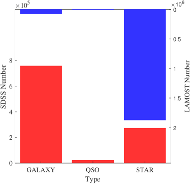
Figure 1.— The comparison of the object types between SDSS DR13 (red) and LAMOST DR4 (blue) spectroscopic survey.

2.2. SDSS and $WISE$ Photometric Surveys

The combination of optical and infrared (IR) data on huge numbers has been proved to be valid in the star/galaxy classification (Baldry et al., 2010; Henrion et al., 2011) and stellar parameter determination (Allende Prieto, 2016). The SDSS has imaged over 31 thousand square degrees in five broad bands ($ugriz$). The DR13 includes photometry for over one billion objects. The Wide-field Infrared Survey Explorer ($WISE$; Wright et al. 2010), performed an all-sky survey with images in 3.4, 4.6, 12 and 22 $\mu$m and yielded more than half a billion objects.

In order to obtain the training sample, we extract the objects with the available model magnitudes in $g$, $r$, $i$ bands for the SDSS and LAMOST spectroscopic surveys, and cross identify them with the $WISE$ All-Sky Data Release catalog with the help of the Catalog Archive Server Jobs (CasJobs). Similar to (Krakowski et al., 2016), we use w1(2)mpro magnitudes. The $J$, $H$, and $K$ magnitudes are also extracted in order to cover the near IR bands. Our selection required the object with zWarning = 0 for the SDSS objects, and S/N ratios higher than 2 in the $W$1 and $W$2 bands. We adopt the w?mag13 as the indicators for the extended objects (Bilicki et al., 2014; Krakowski et al., 2016; Kurcz et al., 2016; Solarz et al., 2017), which is defined as

$$\mathrm{w?mag13}=\mathrm{w?mag\_1}-\mathrm{w?mag\_3},$$ (1)

where w$?$mag_1 and w$?$mag_3 are magnitudes measured with circular apertures of radii of 5.5″ and 11″. The question mark is the channel number in the catalog.

3. Star/Galaxy/QSO Classification

Classification lies at the foundation of astronomy, and it is the beginning of understanding the relationships between disparate groups of objects and identifying the truly peculiar ones (Gray & Corbally, 2009). In this section, we present the machine-learning method and the performance tests of our classifier.

3.1. Method

We use the CasJobs to cross identify the photometric data with the spectral catalogs of LAMOST, SDSS and Veron13. The result has 2,973,855 objects, included 2,123,831 stars, 806,139 galaxies and 43,885 QSOs. We present the color-color diagram in Figure 2 that is often used for the star-galaxy separation (e.g., Jarrett et al. 2011; Goto et al. 2012; Ferraro et al. 2015). The contours of the three classes overlap in the color-color diagram. Neither the cut $W$1$-W$2 = 0.8 (Stern et al., 2012; Yan et al., 2013), nor $W$1$-J$ = $-$1.7 (Goto et al., 2012) could provide a clear cut to classify the stars, galaxies and QSOs.

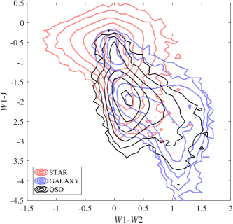
Figure 2.— The color-color diagram for stars (red), galaxies (blue) and QSOs (black) in our training sample.

We build a nine-dimensional color space, $g-r$, $r-i$, $i-J$, $J-H$, $H-K$, $K-W$1, $W$1$-$$W$2, w1mag13, and w2mag13. Each object is weighted with the quadratic sum of their photometric uncertainty. The holdout validation is applied to test the total accuracies of different machine-learning algorithms, in which a random partition of 20% is held out for the prediction and the rest is used to train the classifier.

Table 1 lists the accuracies and time costs of different algorithms for the 20% held out samples. Since the validation is applied, the time costs are approximate. The RF algorithm (Breiman, 2001) shows the best performance on the time cost (57 min ) and the total accuracy (99.2%). Other methods, for example the $k$-nearest neighbor and the SVM, either cost more time to build the classifiers or show lower total accuracies.

Table 1The accuracies and time costs of different algorithms

Algorithm	Accuracy [%]	Time cost1
Simple Tree2	97.6	minutes
Medium Tree3	98.6	minutes
Complex Tree4	98.8	minutes
Linear Discriminant5	98.3	a minute
Quadratic Discriminant6	98.2	a minute
Fine KNN7	98.7	a hour
Medium KNN8	99.1	a hour
Coarse KNN9	99.0	hours
Cosine KNN10	99.0	hours
Cubic KNN11	99.1	hours
Weighted KNN12	99.0	hours
RF	99.2	hours
Linear SVM13	98.9	a week
Quadratic SVM14	90.6	a week
Fine Gaussian SVM14	98.9	a week
Cubic SVM14	72.9	a week
Medium Gaussian SVM14	99.1	a week
Coarse Gaussian SVM14	99.2	a week

Note. — 1. One worker for the parallel computing. 2. Few leaves to make coarse distinctions between classes. 3. Medium number of leaves for finer distinctions between classes. 4. Many leaves to make many fine distinctions between classes. 5. Creates linear boundaries between classes. 6. Creates nonlinear boundaries between classes. 7. Finely detailed distinctions between classes. 8. Medium distinctions between classes. 9. Coarse distinctions between classes. 10. Medium distinctions between classes, using a Cosine distance metric. 11. Medium distinctions between classes, using a cubic distance metric. 12. Medium distinctions between classes, using a distance weight. 13. Makes a simple linear separation between classes. 14. Makes a nonlinear separation between classes.

The working theory of the RF is that it builds an ensemble of unpruned decision trees and merges them together to get a more accurate and stable prediction. The algorithm consists of many decision trees and outputs the class that is the mode of the class output by individual trees (Breiman, 2001; Gao et al., 2009). The RF are often used when we have very large training datasets and a very large number of input variables. One big advantage of RF is fast learning from a very large number of data. Gao et al. (2009) listed many other advantages of the RF.

After selecting the best algorithm, we apply the holdout validation and test the RF classifier ten times. The average accuracy is 99% and the result is shown in Table 2 and Figure 4. In the classifier, the contributions of the nine colors are different, which could be described by the predictor importance estimates (Figure 3). We find that the IR colors play an important role in our classifier, which is similar to the result of Krakowski et al. (2016).

We adopt the measures defined by Soumagnac et al. (2015) to show the performance of the classifier. These measures have been used in other machine-learning studies (Kovács & Szapudi, 2015; Krakowski et al., 2016): completeness ($c$), and purity ($p$) for star, galaxy and QSO samples. We use the following equations (here for galaxies):

$$c_{g}=\frac{\textrm{TG}}{\textrm{TG+FGS+FGQ}},$$ (2)

$$p_{g}=\frac{\textrm{TG}}{\textrm{TG+FSG+FQG}}.$$ (3)

The FGS and FGQ are the numbers of galaxies misclassified as stars and QSOs, and FSG and FQG are the numbers of stars and QSOs misclassified as galaxies. The QSO sample shows the lowest completeness and purity, probably due to its smallest sample size.

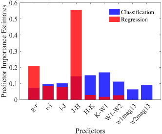
Figure 3.— The predictor importance estimates for the classification and the regression.

In order to test this effect, we normalize the sample sizes of the three classes, and apply the 20% holdout validation again (about 8,800 objects in each type for the testing). The average result is shown in the Table 2 and the right panel of Figure 4. The three classes have similar percentages of the completeness and purity. This result implies that we could not judge the performance of the classifier only by these measures.

We also apply the magnitude binnings suggested by (Krakowski et al., 2016) to test the completeness, since different magnitudes stand for different stellar and galactic types and distances. The binnings are 12 $<W$1 $<$ 13, 13 $<W$1 $<$ 14, 14 $<W$1 $<$ 15, and 15 $<W$1 $<$ 16. The completenesses for stars, galaxies and QSOs are similar to those calculated without binning. On the even samples, the low performance of the galaxy sample is probably due to the relatively high contamination from the QSO sample rather than the lost information of the galaxy sample.

Table 2The comparison of the average performance

	All Samples		Uniform Samples
	$c$ [%]	$p$ [%]	$c$ [%]	$p$ [%]
Stars	99.6	99.7	99.6	96.5
Galaxies	98.9	97.8	97.6	92.5
QSOs	71.9	88.5	88.9	97.4
Accuracy	99		95

Note. — All samples: the classifier using all samples. Uniform samples: the classifier using samples with the same numbers of the different classes. $c$ = completeness, and $p$ = purity.

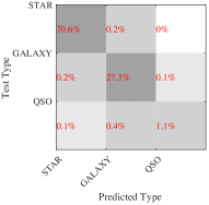
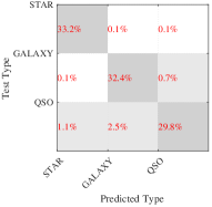
Figure 4.— The comparison of the confusion matrixes for two classifiers: one using all samples and the other using samples with the same numbers of the different classes.

3.2. Blind Test

This section describes various tests using the classifier made from the LAMOST, SDSS and Veron13. These tests allow us to quantify the performance of the classification.

3.2.1 6dF Galaxy Survey

The 6dF Galaxy Survey has (6dFGS) mapped the nearby universe over nearly half the sky (Jones et al., 2004, 2009). The final redshift release of the 6dFGS contains 124,647 spectrally identified galaxies. We match the galaxies with the SDSS and $WISE$ archive data, which yields 12,300 galaxies. We then remove the galaxies which are used to build the classifier, and there are 8,382 galaxies left. We feed the classifier with nine colors of these galaxies, and obtain the predicted types. The classifier can output three scores for each entry, corresponding to the possibilities for star, the galaxy and the QSO. The type with the largest score is adopted as the predicted type. The classifier also output the standard deviation ($\sigma$) for each score.

About 99.5% of the galaxies are classified correctly, and 40 galaxies are wrongly classified as stars. Here all the predicted QSOs are treated as the galaxies, since there is no QSO subtype in the 6dFGS. The classification result is shown in Figure 5. The scores of the correctly classified galaxies are larger than those of the wrongly classified. About 73% of the correctly classified galaxies have $\sigma<$ 0.2, while only 55% for the wrongly classified galaxies have $\sigma<$ 0.2. It indicates that the classifier is very uncertain about the types of the wrongly classified galaxies.

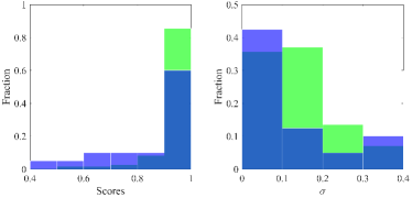
Figure 5.— The classification result of the 6dFGS. Left panel: the distribution of the scores for correctly classified galaxies (green) and wrongly classified galaxies (blue). The one score means 100 percent. Right panel: the distribution of the scores’ standard deviation.

3.2.2 RAVE

The RAdial Velocity Extension (RAVE) is designed to provide stellar parameters to complement missions that focus on obtaining radial velocities to study the motions of stars in the Milky Way s thin and thick disk and stellar halo (Steinmetz et al., 2006). Its fifth data release (DR5) contains 457,588 stars in the south sky (Kunder et al., 2017). There are 935 stars also observed by SDSS and $WISE$. We remove the stars used to build the classifier, and there are 737 stars left. We feed the classifier with the nine colors and it yields 736 stars and one QSO with the accuracy of 99.9%. The wrongly classified star, SDSS J154142.28-194513.1, is located in the bright halo of the kap Lib. Its colors probably be polluted by the bright star.

We also take advantage the $g$, $r$ and $i$ magnitudes from APASS (Munari et al., 2014) that has been matched with RAVE stars (Kunder et al., 2017). Not all the stars are detected in both $WISE$ and APASS, and there are 435,012 stars with valid seven colors. The prediction contains 434,735 stars, 264 galaxies and 13 QSOs with the accuracy of accuracy 99.9%. The classification result is shown in Figure 6. The wrongly classified Stars have smaller scores and larger $\sigma$, implying the high uncertainty of the types.

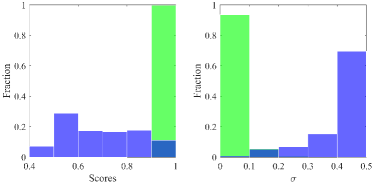
Figure 6.— The classification result of the APASS-RAVE. Left panel: the distribution of the scores for correctly classified stars (red) and wrongly classified stars (blue). Right panel: the distribution of the scores’ standard deviation.

3.2.3 UVQS

The data release one of all-sky UV-bright Quasar Survey (UVQS) contains 1,055 QSOs selected from $GALEX$ and $WISE$ photometry and identified with optical spectra (Monroe et al., 2016). We cross identified the QSOs with SDSS and $WISE$, which yields 262 QSOs. We remove the QSOs used to build the classifier, and there are 237 QSOs left. The classifier yields 224 QSOs, 12 galaxies and one star with the accuracy of 94.5%. Again, the wrongly classified QSOs show smaller scores and larger $\sigma$ (Figure 7). The accuracies of the blind tests is summarized in Table 3.

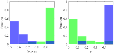
Figure 7.— The classification result of the UVQS. Left panel: the distribution of the scores for correctly classified QSO (green) and wrongly classified QSOs (blue). Right panel: the distribution of the scores’ standard deviation.

Table 3The accuracies of the blind test

Survey	Accuracy
6dFGS	99.5%
RAVE	99.9%
UVQS	94.5%

4. Effective Temperature Regression

We need more information on stars, after separating them from galaxies and QSOs. The stellar spectral classification organizes vast quantities of diverse stellar spectra into a manageable system, and has served as the fundamental reference frame for the studies of stars for over 70 years (Gray & Corbally, 2009). In this section, we present the method and the tests of our regression.

4.1. Method

The LAMOST s 1D pipeline only provides rough classification results and the accuracy of the subclasses is still not robust (Jiang et al., 2013). Therefore, we instead adopt the effective temperatures ($T_{\mathrm{eff}}$) from the A, F, G and K type star catalog, which was produced by the LAMOST stellar parameter pipeline (LASP; Wu et al. 2014). We also extract the $T_{\mathrm{eff}}$ computed with the SEGUE Stellar Parameter Pipeline in the SDSS (SSPP; Allende Prieto et al. 2008; Lee et al. 2008a; 2008b). Both samples are dominated by G stars, and have similar distributions of $T_{\mathrm{eff}}$ (Figure 8).

In the classification (Secion 3), the RF exhibits advantage in the accuracy and the training time cost. We here also adopt the algorithm of RF to build the regression of stellar effective temperature.

These temperatures and seven colors, $g-r$, $r-i$, $i-J$, $J-H$, $H-K$, $K-W$1 and $W$1$-$$W$2, of 1,327,071 stars are used to train the RF for regression. We apply the 10-fold cross validation in order to test the performance of the regression. The cross validation partitions the sample into ten randomly chosen folds of roughly equal size. One fold is used to validate the regression that is trained using the remaining folds. This process is repeated ten times such that each fold is used exactly once for validation.

We present the result of the cross validation in Figure 9. The one-to-one correlation is shown in the left panel. In order to estimate the uncertainty of the prediction, we bin the predicted $T_{\mathrm{eff}}$ with a step size of 100 K, and fit the distribution of the corresponding test $T_{\mathrm{eff}}$ with a Gaussian function. We calculate the root-sum square of the standard deviation and the offset of the fit, which is adopted as the uncertainty of the prediction (the blue error bars in Figure 9). The Gaussian fit to the total residuals is shown in the right panel of Figure 9, and the fitted offset ($\mu$) and the $\sigma$ are listed in Table 4. The red bars in Figure 3 are the importance estimates for the regression. The optical and 2MASS colors show much more importance than the $WISE$ colors, which are different from those of the classification. It may be due to the majority of our sample that is G and K-type stars.

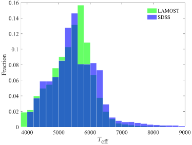
Figure 8.— The normalized distribution of the $T_{\mathrm{eff}}$. The green bars are the training sample of the LAMOST and the blue bars are that of the SDSS.

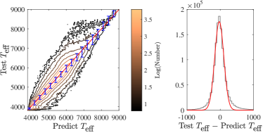
Figure 9.— The one-one correlation of the regression (left panel). The blue error bars stand for the root-sum square of the standard deviation and the offset of the Gaussian fit in the bins of the predicted $T_{\mathrm{eff}}$. The color bar stands for the color of the density contour in the log scale. The Gaussian fit (red) of the total residual (black) is shown in the right panel.

4.2. Blind Test

In this subsection, we use the $T_{\mathrm{eff}}$ extracted from the spectrum-based methods to test the actual performance of the regression.

4.2.1 RAVE

The RAVE pipeline processes the RAVE spectra and derives estimates of $T_{\mathrm{eff}}$, log $g$, and [Fe/H] (Kunder et al., 2017). The pipeline is based on the combination of the MATrix Inversion for Spectral SynthEsis (MATISSE; Recio-Blanco et al. 2006) algorithm and the DEcision tree alGorithm for AStrophysics (DEGAS; Bijaoui et al. 2012). This pipeline is valid for stars with temperatures between 4000 K and 8000 K. The estimated errors in $T_{\mathrm{eff}}$ is approximately 250 K, and $\sim$ 100 K for spectra with S/N $\sim$ 50 (Kunder et al., 2017).

We adopt the photometry from APASS and $WISE$ in the RAVE database to construct the input colors. The sample is restricted to have S/N $\geqslant$ 50 and the quality flag of $Algo\_Conv$ $\neq$ 3 or 4 . There are 165,011 stars left. We present the prediction result in Figure 10, and list the parameters of the Gaussian fit to the total residuals in Table 4.

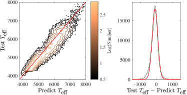
Figure 10.— The one-one correlation of the stars in the APASS-RAVE (left panel). The Gaussian fit (red) of the total residual (black) is shown in the right panel.

4.2.2 APOGEE

The Apache Point Observatory Galactic Evolution Experiment (APOGEE), one of the programs in SDSS-III, has collected high-resolution ($R$ $\sim$ 22,500) high signal-to-noise ($>$ 100) near-infrared (1.51$-$1.71 $\mu$m) spectra of 146,000 stars across the Milky Way (Majewski et al., 2017). These stars are dominated by red giants selected from the 2MASS. Their stellar parameters and chemical abundances are estimated by the APOGEE Stellar Parameters and Chemical Abundances Pipeline (ASPCAP; García Pérez et al. 2016). The typical error in $T_{\mathrm{eff}}$ is $\sim$ 100 K (Mészáros et al., 2013).

We extract the photometric data of SDSS and $WISE$ with the help of the Casjob. We feed the RF regression with the seven colors of 13,685 stars. The prediction is shown in Figure 11, and the parameters of fit to the total residuals are listed in Table 4.

We find that the offsets of the validation and the predictions are less than 100 K, and the standard deviations are less than 200 K (Figure 10 and 11). Lee et al. (2015) has applied the SSPP to LAMOST stars and compared the results to those from RAVE and APOGEE catalogs. The offsets of $T_{\mathrm{eff}}$ between different pipelines are from 36 to 73 K and the standard deviations are from 79 to 172 K. This indicates that our RF regression can determine the stellar temperatures with fair accuracy.

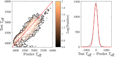
Figure 11.— The one-one correlation of the stars in the APOGEE (left panel). The Gaussian fit (red) of the total residual (black) is shown in the right panel.

Table 4The Gaussian fits to the total residuals.

	$\mu$	$\sigma$
	(K)	(K)
Cross Validation	$-$27 $\pm$ 2	136 $\pm$ 2
RAVE	$-$93 $\pm$ 3	175 $\pm$ 3
APOGEE	$-$36 $\pm$ 2	182 $\pm$ 2

5. Discussion

The machine learning has been adopted as a successful alternative approach to defining reliable objects classes, stellar types and types of variable stars (eg. Liu et al. 2015; Kovács & Szapudi 2015; Krakowski et al. 2016; Kuntzer et al. 2016; Sarro et al. 2018; Pashchenko et al. 2018). It is not the first time to take advantage of this technology to classify the objects or to regress the stellar parameters. In this section, we would like to compare our classification and regression to the results in other studies.

5.1. Comparisons with other machine-learning methods

Ball et al. (2006) applied the supervised decision tree algorithm to classify the stars and galaxies in SDSS-DR3. They used the colors $u-g$, $g-r$, $r-i$ and $i-z$ of 477,068 objects with spectroscopic attributes to train the machine-learning classifier, and performed cross validation to test the performance. The accuracy and completeness were over 90%. Except for the optical colors, the IR colors are included in our multi-color data set, since they have shown the importance in the machine-learning methods (Henrion et al., 2011). Our larger training sample and the IR aided color set result in a better performance of our classifier, over 99% for the stars and galaxies classification. We also test the performance of some decision tree algorithms, and the accuracies are $\sim$ 98%. Compared to the decision tree, the random forest avoid overfitting to the training set and limit the error from the bias (Hastie et al., 2008).

Krakowski et al. (2016) used the SVM learning algorithm to classify $WISE$ $\times$ SuperCOSMOS objects based on the SDSS spectroscopic sources. The training sample included over one million objects, 95% of which were galaxies, 2% were stars, and 3% were QSOs. They used six parameters, $W$1, $W$3, $W$1$-$$W$2, $R-$$W$1, $B-R$ and w1mag13. The 10-fold cross validation was performed to test the classifier, and the total accuracy was 97.3%. Instead of magnitudes, we adopt colors that are independent of distance. Our training sample shows better compositional balance, and its size is three times larger than theirs. We also try some SVM algorithms, and the accuracies are from 70% to 99%. The time cost to build the SVM classifier is extremely longer than that for the RF classifier . For a classification problem, the RF gives probability of belonging to classes (Breiman, 2001), while the SVM relies on the concept of ”distance” between points that needs more time to calculate. The RF algorithm also shows better performance than the SVM in other fields, such as Liu et al. (2013).

Liu et al. (2015) employed an SVM-based classification algorithm to predict MK classes with 27 line indices measured from a small sample, 3,134 LAMOST stellar spectra. The holdout validation of 50% was performed to test the accuracy of the classifier. The completeness of A and G stars reached 90%, while that of other stars was below 80%. Since the spectral features of different types can be very similar, clear cuts of these features probably lead to mis-classification. Therefore, we adopt the regression of $T_{\mathrm{eff}}$ rather than the MK classification in order to avoid such effect. Liu et al. (2015)’s research also implies that a large sample could cover a larger area of the parameter space, and further could yield more reliable prediction.

Sarro et al. (2018) constructed regression models to predict $T_{\mathrm{eff}}$ of M stars with eight machine-learning algorithms. The training sample is built with the features extracted from the BT-Settl of synthetic spectra. Then, the models were applied to two sets of real spectra from the NASA Infrared Telescope Facility and Dwarf Archives collections. Sarro et al. (2018) used the root mean/median square errors (RMSE/RMDSE) to describe the prediction errors. The RMSEs were from 160 to 390 K, and the RMDSEs from 90 to 220 K, various with the different algorithms and signal-to-noise ratios. Our prediction for A, F, G, K stars gives similar results: RMSE/RMDSE (RAVE) = 246/140 K, and RMSE/RMDSE (APOGEE) = 247/130 K, implying that our regression built with photometric data could achieve similar accuracy to the spectrum-based model.

5.2. SED Fit

Another way to determine the $T_{\mathrm{eff}}$ is the fit of stellar SEDs with synthetic templates. The theocratical study has concluded that the broad-band photometry from the UV to the mid-IR allows atmospheric parameters and interstellar extinction to be determined with good accuracy (Allende Prieto, 2016). The study used the SEDs extracted from the ATLAS9 model atmospheres (Mészáros et al., 2012). They added interstellar extinction to these SEDs in order to construct the theocratical templates. The test SEDs were also extracted from the ATLAS9 model, but added some random noise. Then the test SEDs were fitted with the templates using the $\chi^{2}$-optimization method. The standard deviations of the total residual were from 130 to 380 K depending on different bands used for the fittings. We follow this procedure to fit 10⁵ simulated SEDs, extracted from the BT-Cond theoretical model (Baraffe et al., 2003; Barber et al., 2006; Allard & Freytag, 2010). Since the simulated SEDs have random stellar parameters, about 70,000 SEDs are located inside the reasonable ranges. The result is shown in the upper panels in Figure 12. We only plot $\sim$ 64,000 samples with $\chi^{2}$ $\leqslant$ 5.88 that is one standard deviation for a $\chi^{2}$ distribution with the five degrees of freedom ($T_{\mathrm{eff}}$, log $g$, [Fe/H], $E(B-V)$ and the scaling factor). The residuals are fitted with a Gauss-like function:

$$f=Ae^{\frac{-(x-\mu)^{\delta}}{\delta\sigma^{\delta}}}.$$ (4)

The standard deviation of $T_{\mathrm{eff}}$ is 207 $\pm$ 15 K for 12 bands fit, F-NUV, $ugriz,JHK,W1W2$. The standard deviation of other parameters are also similar to the result in Allende Prieto (2016), indicating that the multi-band SED fit can well constrain the atmospheric parameters and interstellar extinction theocratically.

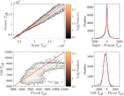
Figure 12.— The results for the theoretical simulation (the upper panels) and the application to LSS-GAC catalog (the lower panels). The color bars stand for the colors of the density contours. We use the Gauss-like function (the red line) to fit the total residual of the theoretical simulation, and use the Gaussian function to fit the residual of the stars in the LSS-GAC catalog.

However, the result is worse than expected (the lower panels in Figure 12), when we apply the SED templates to fit the SEDs in the real observation, the stars in the LAMOST Spectroscopic Survey of the Galactic Anticentre (LSS-GAC; Liu et al. 2014; Yuan et al. 2015). The standard deviation of $T_{\mathrm{eff}}$ is 454 $\pm$ 5 K and the offset is $-$365 $\pm$ 5 K, larger than those of the machine-learning regression by a factor of three. We also try this technology in other ways, e.g., fitting the stars in RAVE, or using 10 bands fit . The standard deviations of $T_{\mathrm{eff}}$ are about 400 K, extremely worse than both the theoretical simulation and the machine-learning regression. This implies that the atmospheric parameters of the stars in the real observation can’t be well estimated by the SED fit using the $\chi^{2}$ minimization. Based on photometric data, machine learning shows better performance on the $T_{\mathrm{eff}}$ estimate.

5.3. A Scientific Application

The ESA space mission $Gaia$ is performing an all-sky survey at optical wavelengths, and its primary objective is to survey more than one billion stars (Gaia Collaboration et al., 2016). Its second data release ($Gaia$ DR2; Gaia Collaboration et al. 2018) includes $\sim$ 1.3 billion objects with valid parallaxes. These parallaxes are obtained with a complex iterative procedure, involving various assumptions (Lindegren et al., 2012). Such procedure may produce parallaxes for galaxies and QSOs, which should present no significant parallaxes (Liao et al., 2018).

We have applied the classifier to 85,613,922 objects in the $Gaia$ DR2 based on the multi-wavelength data from Pan-STARRS and $WISE$ (Bai et al., 2018b). The result shows that the sample is dominated by stars, $\sim$ 98%, and galaxies and QSOs make up 2%. For the objects with negative parallaxes, about 2.5% are galaxies and QSOs. About 99.9% of the sample are stars if the relative parallax uncertainties are smaller than 0.2, implying that using the threshold of 0 $<\sigma_{\pi}/\pi<$ 0.2 could yield a very clean stellar sample (Bai et al., 2018b).

6. Summary and Future Work

In this work we have attempted to classify the objects into stars, galaxies and QSOs, and further regress the effective temperatures for stars using the machine learning, the algorithm of choice being the RF. The classifier is trained with about three million objects in SDSS, LAMOST and Veron13, and the regression is trained with one million stars in SDSS and LAMOST. In order to exam the performance of the classifier, we perform three blind tests by using objects spectroscopically identify in the RAVE, 6dFGS, and UVQS. The total accuracies are over 99% for the RAVE and 6dFGS, and higher than 94% for the UVQS. We also perform two blind tests for the regression by using the stellar $T_{\mathrm{eff}}$ estimated with spectroscopical pipelines in the RAVE and APOGEE. The offsets and the standard deviations of the total residual are below 100 K and 200 K, respectively.

Our classifier shows the high accuracy compared to other machine-learning algorithms in former studies, indicating that combining broad-band photometry from the optical to the mid-infrared allows classification to be determined with very high accuracy. The machine learning provides us an efficient approach to determine the classes for huge amounts of objects with photometric data, e.g., over four hundred million objects in the SDSS-$WISE$ matched catalog.

Since there is no clear cut for colors or spectral features of the different spectral types, we adopt $T_{\mathrm{eff}}$ regression rather than the MK classification to further provide basic information on stars. Our regression result shows similar or even better performance than the SED $\chi^{2}$ minimization and some spectrum-based methods. The RF regression enable us to estimate the $T_{\mathrm{eff}}$ without spectral data for the stars that are too many or too faint for the spectral observation, or the stars in the large area time dominated survey (e.g., Pan-STARRS1 survey; Chambers et al. 2016).

We are going to test regressions for other stellar parameters with machine-learning algorithms. We also try to decouple the effective temperature and the interstellar extinction based on large sample, such as LAMOST-SDSS-Gaia. The future well controlled sample, e.g., LAMOST-II and SDSS-V (Kollmeier et al., 2017), also provides us an opportunity to explore the multi-dimensional parameter space with this technology for classification and regression.

The machine-learning results in this work are developed with MATLAB available upon request to the first author as MAT files.

References

- Albareti et al. (2017) Albareti, F. D., Allende Prieto, C., Almeida, A., et al. 2017, ApJS, 233, 25
- Allard & Freytag (2010) Allard, F., & Freytag, B. 2010, Highlights of Astronomy, 15, 756
- Allende Prieto (2016) Allende Prieto, C. 2016, A&A, 595, A129
- Allende Prieto et al. (2008) Allende Prieto, C., Sivarani, T., Beers, T. C., et al. 2008, AJ, 136, 2070
- Bai et al. (2018a) Bai, Y., Liu, J.F., Wicker, J., et al. 2018, ApJS, 235, 16
- Bai et al. (2018b) Bai, Y., Liu, J.-F., & Wang, S. 2018, Research in Astronomy and Astrophysics, 18, 118
- Bailer-Jones et al. (2013) Bailer-Jones, C. A. L., Andrae, R., Arcay, B., et al. 2013, A&A, 559, A74
- Baldry et al. (2010) Baldry, I. K., Robotham, A. S. G., Hill, D. T., et al. 2010, MNRAS, 404, 86
- Ball et al. (2006) Ball, N. M., Brunner, R. J., Myers, A. D., & Tcheng, D. 2006, ApJ, 650, 497
- Baraffe et al. (2003) Baraffe, I., Chabrier, G., Barman, T. S., Allard, F., & Hauschildt, P. H. 2003, A&A, 402, 701
- Barber et al. (2006) Barber, R. J., Tennyson, J., Harris, G. J., & Tolchenov, R. N. 2006, MNRAS, 368, 1087
- Bilicki et al. (2014) Bilicki, M., Jarrett, T. H., Peacock, J. A., Cluver, M. E., & Steward, L. 2014, ApJS, 210, 9
- Bijaoui et al. (2012) Bijaoui, A., Recio-Blanco, A., de Laverny, P., & Ordenovic, C. 2012, StMet, 9, 55
- Bolton et al. (2012) Bolton, A. S., Schlegel, D. J., Aubourg, É., et al. 2012, AJ, 144, 144
- Blanton et al. (2017) Blanton, M. R., Bershady, M. A., Abolfathi, B., et al. 2017, AJ, 154, 28
- Breiman (2001) Breiman, L. 2001, in Random Forests, 45, pp 5-32
- Chambers et al. (2016) Chambers, K. C., Magnier, E. A., Metcalfe, N., et al. 2016, arXiv:1612.05560
- Christianini & J. C. Shawe-Taylor (2000) Christianini, N., & J. C. Shawe-Taylor, 2000, An Introduction to Support Vector Machines and Other Kernel-Based Learning Methods. Cambridge, UK: Cambridge University Press
- Cortes & Vapnik (1995) Cortes, C., & Vapnik, V., 1995, Machine Learning, 20, 273
- Cui et al. (2012) Cui, X.-Q., Zhao, Y.-H., Chu, Y.-Q., et al. 2012, Research in Astronomy and Astrophysics, 12, 1197
- Daniel et al. (2011) Daniel, S. F., Connolly, A., Schneider, J., Vanderplas, J., & Xiong, L. 2011, AJ, 142, 203
- Deng et al. (2012) Deng, L.-C., Newberg, H. J., Liu, C., et al. 2012, Research in Astronomy and Astrophysics, 12, 735
- Ferraro et al. (2015) Ferraro, S., Sherwin, B. D., & Spergel, D. N. 2015, Phys. Rev. D, 91, 083533
- Fix & Hodges (1951) Fix, E., & Hodges, J. L., 1951, Discriminatory analysis, nonparametric discrimination: consistency properties. Tech. Rep. 4, USAF School of Aviation Medicine, Randolph Field, Texas
- Gaia Collaboration et al. (2016) Gaia Collaboration, Prusti, T., de Bruijne, J. H. J., et al. 2016, A&A, 595, A1
- Gaia Collaboration et al. (2018) Gaia Collaboration, Brown, A. G. A., Vallenari, A., et al. 2018, arXiv:1804.09365
- Gao et al. (2009) Gao, D., Zhang, Y.-X., & Zhao, Y.-H. 2009, Research in Astronomy and Astrophysics, 9, 220
- Garcia-Dias et al. (2018) Garcia-Dias, R., Allende Prieto, C., Sánchez Almeida, J., & Ordovás-Pascual, I. 2018, arXiv:1801.07912
- García Pérez et al. (2016) García Pérez, A. E., Allende Prieto, C., Holtzman, J. A., et al. 2016, AJ, 151, 144
- Goto et al. (2012) Goto, T., Szapudi, I., & Granett, B. R. 2012, MNRAS, 422, L77
- Gray & Corbally (2009) Gray, R. O., & Corbally, C., J. 2009, Stellar Spectral Classification by Richard O. Gray and Christopher J. Corbally. Princeton University Press
- Hastie et al. (2008) Hastie, T., Tibshirani, R., & Friedman, J. 2008, in The Elements of Statistical Learning, 2nd ed. Springer, pp. 587-588
- Henrion et al. (2011) Henrion, M., Mortlock, D. J., Hand, D. J., & Gandy, A. 2011, MNRAS, 412, 2286
- Huertas-Company et al. (2008) Huertas-Company, M., Rouan, D., Tasca, L., Soucail, G., & Le Fèvre, O. 2008, A&A, 478, 971
- Huertas-Company et al. (2009) Huertas-Company, M., Tasca, L., Rouan, D., et al. 2009, A&A, 497, 743
- Jarrett et al. (2011) Jarrett, T. H., Cohen, M., Masci, F., et al. 2011, ApJ, 735, 112
- Jiang et al. (2013) Jiang, B., Luo, A., Zhao, Y., & Wei, P. 2013, MNRAS, 430, 986
- Jones et al. (2004) Jones, D. H., Saunders, W., Colless, M., et al. 2004, MNRAS, 355, 747
- Jones et al. (2009) Jones, D. H., Read, M. A., Saunders, W., et al. 2009, MNRAS, 399, 683
- Kollmeier et al. (2017) Kollmeier, J. A., Zasowski, G., Rix, H.-W., et al. 2017, arXiv:1711.03234
- Kovács & Szapudi (2015) Kovács, A., & Szapudi, I. 2015, MNRAS, 448, 1305
- Krakowski et al. (2016) Krakowski, T., Małek, K., Bilicki, M., et al. 2016, A&A, 596, A39
- Kurcz et al. (2016) Kurcz, A., Bilicki, M., Solarz, A., et al. 2016, A&A, 592, A25
- Kunder et al. (2017) Kunder, A., Kordopatis, G., Steinmetz, M., et al. 2017, AJ, 153, 75
- Kuntzer et al. (2016) Kuntzer, T., Tewes, M., & Courbin, F. 2016, A&A, 591, A54
- Lee et al. (2008a) Lee, Y. S., Beers, T. C., Sivarani, T., et al. 2008a, AJ, 136, 2022
- Lee et al. (2008b) Lee, Y. S., Beers, T. C., Sivarani, T., et al. 2008b, AJ, 136, 2050
- Lee et al. (2015) Lee, Y. S., Beers, T. C., Carlin, J. L., et al. 2015, AJ, 150, 187
- Liao et al. (2018) Liao, S.-l., Qi, Z.-x., Guo, S.-f., & Cao, Z.-h. 2018, arXiv:1804.08821
- Lindegren et al. (2012) Lindegren, L., Lammers, U., Hobbs, D., et al. 2012, A&A, 538, A78
- Liu et al. (2015) Liu, C., Cui, W.-Y., Zhang, B., et al. 2015, Research in Astronomy and Astrophysics, 15, 1137
- Liu et al. (2013) Liu, M., Wang, M., Wang, J. & Li, D., 2013, Sensors and Actuators B: Chemical, 177, 970
- Liu et al. (2014) Liu, C., Deng, L.-C., Carlin, J. L., et al. 2014, ApJ, 790, 110
- Luo et al. (2015) Luo, A.-L., Zhao, Y.-H., Zhao, G., et al. 2015, Research in Astronomy and Astrophysics, 15, 1095
- Majewski et al. (2017) Majewski, S. R., Schiavon, R. P., Frinchaboy, P. M., et al. 2017, AJ, 154, 94
- Manteiga et al. (2009) Manteiga, M., Carricajo, I., Rodríguez, A., Dafonte, C., & Arcay, B. 2009, AJ, 137, 3245
- Mészáros et al. (2012) Mészáros, S., Allende Prieto, C., Edvardsson, B., et al. 2012, AJ, 144, 120
- Mészáros et al. (2013) Mészáros, S., Holtzman, J., García Pérez, A. E., et al. 2013, AJ, 146, 133
- Monroe et al. (2016) Monroe, T. R., Prochaska, J. X., Tejos, N., et al. 2016, AJ, 152, 25
- Munari et al. (2014) Munari, U., Henden, A., Frigo, A., et al. 2014, AJ, 148, 81
- Navarro et al. (2012) Navarro, S. G., Corradi, R. L. M., & Mampaso, A. 2012, A&A, 538, A76
- Parks et al. (2018) Parks, D., Prochaska, J. X., Dong, S., & Cai, Z. 2018, MNRAS, 476, 1151
- Pashchenko et al. (2018) Pashchenko, I. N., Sokolovsky, K. V., & Gavras, P. 2018, MNRAS, 475, 2326
- Recio-Blanco et al. (2006) Recio-Blanco, A., Bijaoui, A., & de Laverny, P. 2006, MNRAS, 370, 141
- Reis et al. (2018) Reis, I., Poznanski, D., Baron, D., Zasowski, G., & Shahaf, S. 2018, arXiv:1711.00022
- Sarro et al. (2018) Sarro, L. M., Ordieres-Meré, J., Bello-García, A., González-Marcos, A., & Solano, E. 2018, MNRAS, 476, 1120
- Solarz et al. (2017) Solarz, A., Bilicki, M., Gromadzki, M., et al. 2017, A&A, 606, A39
- Soumagnac et al. (2015) Soumagnac, M. T., Abdalla, F. B., Lahav, O., et al. 2015, MNRAS, 450, 666
- Steinmetz et al. (2006) Steinmetz, M., Zwitter, T., Siebert, A., et al. 2006, AJ, 132, 1645
- Stern et al. (2012) Stern, D., Assef, R. J., Benford, D. J., et al. 2012, ApJ, 753, 30
- Suchkov et al. (2005) Suchkov, A. A., Hanisch, R. J., & Margon, B. 2005, AJ, 130, 2439
- Vasconcellos et al. (2011) Vasconcellos, E. C., de Carvalho, R. R., Gal, R. R., et al. 2011, AJ, 141, 189
- Véron-Cetty & Véron (2010) Véron-Cetty, M.-P., & Véron, P. 2010, A&A, 518, A10
- Weir et al. (1995) Weir, N., Fayyad, U. M., & Djorgovski, S. 1995, AJ, 109, 2401
- Wu et al. (2014) Wu, Y., Du, B., Luo, A.L., et al. 2014, IAUS, 306, 340
- Wright et al. (2010) Wright, E. L., Eisenhardt, P. R. M., Mainzer, A. K., et al. 2010, AJ, 140, 1868-1881
- Yan et al. (2013) Yan, L., Donoso, E., Tsai, C.-W., et al. 2013, AJ, 145, 55
- Yi et al. (2014) Yi, Z., Luo, A., Song, Y., et al. 2014, AJ, 147, 33
- Yuan et al. (2015) Yuan, H.-B., Liu, X.-W., Huo, Z.-Y., et al. 2015, MNRAS, 448, 855
- Zhao et al. (2012) Zhao, G., Zhao, Y.-H., Chu, Y.-Q., Jing, Y.-P., & Deng, L.-C. 2012, Research in Astronomy and Astrophysics, 12, 723