Witnessing quantum memory in non-Markovian processes
We present a method to detect quantum memory in a non-Markovian process. We call a process Markovian when the environment does not provide a memory that retains correlations across different system-environment interactions. We define two types of non-Markovian processes, depending on the required memory being classical or quantum. We formalise this distinction using the process matrix formalism, through which a process is represented as a multipartite state. Within this formalism, a test for entanglement in a state can be mapped to a test for quantum memory in the corresponding process. This allows us to apply separability criteria and entanglement witnesses to the detection of quantum memory. We demonstrate the method in a simple model where both system and environment are single interacting qubits and map the parameters that lead to quantum memory. As with entanglement witnesses, our method of witnessing quantum memory provides a versatile experimental tool for open quantum systems.
1 Introduction
In any quantum device, the system that carries the information unavoidably interacts with its environment introducing noise. Studying the dynamics of such system-environment interactions is the field of open quantum systems Breuer and it is nowadays more relevant than ever. As quantum devices begin to demonstrate an advantage over classical ones Arute2019, they increasingly rely on Noisy Intermediate-Scale Quantum (NISQ) technology, whose main challenge is noise Preskill2018.
Noise models typically rely on the assumption of Markovianity, i.e., that the environment does not keep memory of past interactions with the system. However, this assumption typically fails in realistic scenarios, as information stored in the environment can keep track of past interactions with the system and affect its future dynamics. For example, this was demonstrated to occur in the IBM quantum computing platform morris2019. In the study of such memory effects, an important distinction is whether the memory can be represented classically or requires genuinely quantum degrees of freedom. The two scenarios can lead to radically different noise models and strategies to compensate it. For example, in the presence of classical memory one could monitor the system and correct its evolution through an appropriate classical feedback. However, this method fails for quantum temporal correlations mediated by the environment. It is therefore desirable to find efficient methods to discriminate quantum vs classical memory.
Most models of open quantum systems with memory regard the process as a dynamical map which maps the system from one time-step to the other Piilo08; Wolf2008; Breuer09; Rivas10; Hou11; Chruscinski14; Rivas2014; Breuer16; LI20181; Vega:2017aa. Within this approach, many models of processes with classical memory have been developed Shapiro1987; Caves1987; wiseman1993; budini2001; Zhou2010; BORDONE2012; Bodor2013; Xu2013; Vacchini2013; Budini2018. However, dynamical maps study only two-time correlations (time of input and output of the map) and multi-time-correlations cannot be fully captured. Furthermore, dynamical maps are in general ill-defined in the presence of initial system-environment correlations Shaji2005; Pechukas1994; Stelmachovic2001; Schmid2019, although such correlations can be responsible for non-Markovianity.
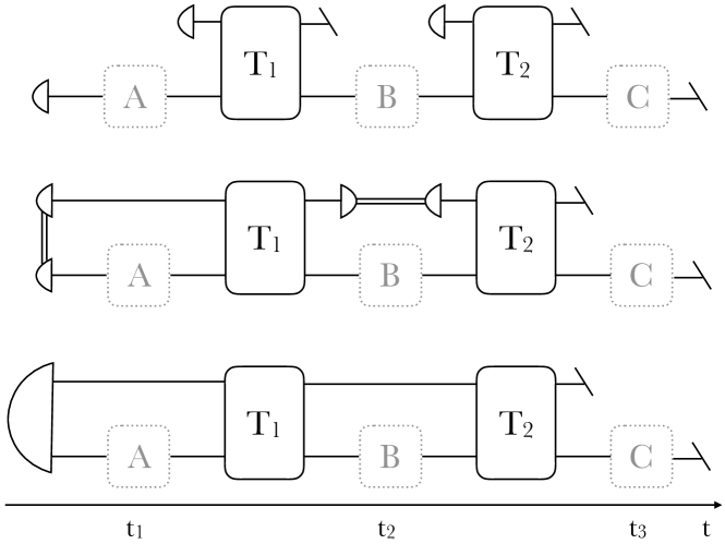
Here, we introduce a definition of quantum process with classical memory based on an approach that captures multi-time correlations, originally introduced by Lindblad Lindblad:1979aa and Accardi et al. Accardi82, and recently reformulated within the comb formalism chiribella09b by Pollock et al. Pollock:2018aa, Fig. 1. We provide a technique to efficiently detect the presence of quantum memory in a non-Markovian process, without requiring full tomography. We use the process matrix formalism Oreshkov12; Oreshkov16 to write the process as a multipartite state. For a specific partition of the state, classical memory implies separability, while entanglement proves quantum memory. Therefore, we can employ all the known techniques that verify entanglement and use them to prove non-Markovianity with quantum memory.
To illustrate our method of detecting quantum memory, we use entanglement witnesses to obtain witnesses for quantum memory for the following toy model: system and environment are qubits jointly prepared in a maximally entangled state and later interact according to the Ising model, in between two measurement stations and for the system. A quantum memory witness corresponds to a set of operations at and . As separability criteria for the search of witnesses we use the positive partial transpose (PPT) applied on the state Peres:1996aa and on symmetric extensions of the state Doherty:2004aa. To find a witness, we cast each criterion as a SemiDefinite Program that can be solved efficiently nesterov87. This also allows us to restrict the search for witnesses, possibly tailored to experimental limitations.
2 Quantum processes
We use the process matrix formalism Oreshkov12; Oreshkov16 to describe quantum processes. We consider a system that evolves through a given sequence of time steps. Each time step can be seen as a “measurement station”, labelled , where an experimenter can intervene on the system, e.g. by measuring or transforming it. Each operation can be represented by a completely positive map (CP) that maps the input system to the output system of the operation. A general intervention on the system is described by a quantum instrument davies70: a collection of CP maps , corresponding to all possible outcomes of a measurement, with being a CP and trace preserving (CPTP) map. The joint probability for observing the outcomes corresponding to maps at the respective measuring stations is given by
| (1) |
where are the Choi matrices jamio72; Choi1975 of the maps respectively, and is the process matrix that lives on the combined Hilbert spaces of all input and output systems. The Choi matrix , isomorphic to a CP map is defined as , where is the identity map, , is an orthonormal basis on and denotes matrix transposition in that basis and some basis of . For the scenarios relevant here, where events are in a fixed causal order, process matrices are identical to quantum combs chiribella09b and process tensors Pollock:2018aa. In turn, these objects correspond to the Choi matrix of a quantum channel with memory Kretschmann2005.
In this language, it was found that the process matrix of a Markovian process, where the state of the environment is reset before each time step (Fig. 1, top), must have the following form costa2016; Giarmatzi:2018aa; Pollock:2018ab,
| (2) |
where is the density matrix of the system before the first time step and is the Choi matrix of a channel , defined as above but without the transposition. This means that a Markovian process can be written as a tensor product of the initial state and the Choi matrices of the different channels that connect the measurement stations. As we will see later, this approach to non-Markovianity takes into account all possible temporal correlations within a quantum process—unlike any other definitions based on dynamical maps which only capture two-time-step correlations.
A non-Markovian process with classical memory is one where, during each system-environment interaction, the environment obtains some classical information about the system, which can affect future such interactions (Fig. 1, middle). In other words, the environment can be simulated as a feedback mechanism, which measures the system at each time step and, conditioned on the outcome, affects the system’s evolution at future times Shapiro1987; Caves1987; wiseman1993. To formalise this definition we describe the evolution between two time steps as a quantum instrument: a collection of CP maps that sum up to a CPTP map. Each instrument can depend on the classical information stored in the environment up to that point, namely on all the previous measurement outcomes. We provide a more detailed definition of processes with classical memory in Appendix A1, together with a characterisation of their process matrices.
The main result, relevant for what follows, is that a process matrix with classical memory is proportional to a separable state. Indeed, we prove in Appendix A1 that a necessary condition for a process matrix with classical memory is that it has the form
| (3) |
where , are positive semidefinite matrices.
A process with quantum memory, on the other hand, is one that does not fall within either of the above categories (Markovian or with classical memory) In such a process (Fig. 1, bottom), the environment preserves coherence across different interactions with the system, in a way that cannot be simulated by a measurement and feedback model.
3 Detecting quantum memory
From Eq. 2 we observe that a Markovian process is a tensor product of a state with the Choi matrix of the channels involved. In what follows we focus on scenarios with two time-steps where operations and can be performed. The output of can be ignored since the only contribution to non-Markovianity stems from the initial system-environment correlations and their later interaction. If such a process has a classical memory, it can be written as . Choi’s theorem Choi1975 ensures that the matrices are positive semidefinite; hence the process matrix can be viewed as a product state, up to normalization. Therefore, can be written as a bipartite separable state , where , .
We can now see that detecting entanglement of the state translates to detecting a quantum memory for the process—if the process cannot be written as a separable state, it cannot be Markovian or with classical memory. Note that quantum memory corresponds to entanglement between and , which is and . This is our main result; we can use known methods of entanglement detection to verify that the environment of a non-Markovian process provides a quantum memory—a feature that has not been explored before. Previous works have connected entanglement with non-Markovianity—for example in Rivas10; Koodynski:2020aa; Chruscinski:2014aa—however, these approaches are based on dynamical maps and therefore, as we discussed, they are insufficient for a full characterisation of non-markovianity. We proceed with the detection method, and discuss later possible applications.
One approach to detecting entanglement is through entanglement witnesses. An entanglement witness is a hermitian operator whose expectation value is positive for all separable states, A negative expectation value guarantees entanglement of the state, whereas a positive value provides no guarantee for separability. In the case of processes, we define a quantum memory witness to be a hermitian operator whose expectation value is positive for all process matrices with classical memory
| (4) |
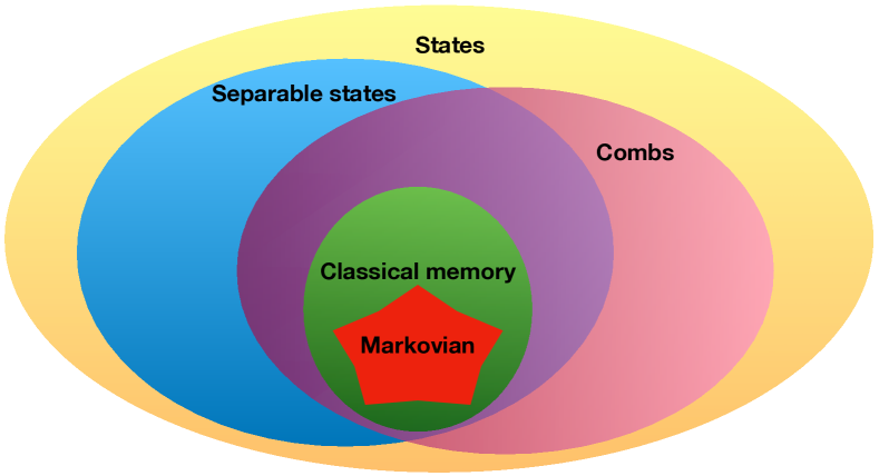
We note that an entanglement witness is also a quantum memory witness for the associated process, but the reverse is not necessarily true. This has to do with the fact that Eq 3 is a necessary condition for a process with classical memory but not sufficient. That is, not any separable state represents a comb. This is because the set of states is larger than the set of combs; see Fig 2. Combs chiribella09b obey further linear constraints , where is a projector on the subspace characterised, e.g., in araujo15. Hence, — is self adjoint.This means that, if L(Z) is an entanglement witness, then Z is also a witness for classical memory, although not necessarily an entanglement witness. Finally, we conjecture that the space of processes with classical memory is strictly smaller than the intersection of combs and separable states. These are in direct analogy to the fact that not all separable channels can be realised through local operations and classical communication Rains1997; Vedral1998; Bennett1999. See Appendix A1 for further discussion.
A quantum memory witness is a hermitian matrix, hence it can always be decomposed into combinations of CP maps araujo15. From Equation 1 we see that the witness corresponds to the different maps of the measurement stations; for example for a bipartite process,
| (5) |
Crucially, measuring the witness only requires performing the CP maps in (5) and does not require full process tomography. This makes the technique suitable for experiments, similarly to witnesses for indefinite causal order Rubinoe1602589; Goswami2018.
We note that detecting a quantum memory in an experimental setup is a procedure similar to that of detecting entanglement. First we need a good guess of the realised process matrix. We proceed by finding a witness of quantum memory, that is, an operator consisting of general quantum operations within the process. Experimentally, a negative expectation value of this operator detects quantum memory.
Given the several approaches to non-Markovianity, based on dynamical maps rather than on process matrices, one might wonder if these could also provide a way to witness quantum memory. As we prove in Appendix A2, this is not the case.
3.1 Separability criteria
An entanglement witness is obtained through various separability criteria: a property that is proved to hold for all separable states. These criteria provide necessary (but not sufficient) conditions for a state to be separable. The most notable criterion is based on partial transposition: if a state is separable, it must have a positive partial transpose (PPT) Peres:1996aa with respect to any subsystem. For example, for a bipartite state it is separable if (but not only if) where denotes partial transposition with respect to subsystem ( is an equivalent condition, but is superfluous since positivity of and implies positivity of ). An entanglement witness is obtained through the eigenvector corresponding to the negative eigenvalue of . If , there exists such that . Then is an entanglement witness as its expectation value is negative for the state and positive for any separable state Peres:1996aa
| (6) |
A different family of separability criteria was introduced by Doherty et al. Doherty:2004aa. These criteria are based on the PPT criterion applied on symmetric extensions of the state. For example, for , one can apply the PPT criterion to the extended state and obtain the following necessary conditions for the state to be separable:
| (7) |
One can keep extending the state (i.e. ) and obtain new families of conditions, each at least as strong as the previous ones. This creates a hierarchy of families of separability criteria which was proven to be complete—for an entangled state it is guaranteed that some level of the hierarchy will prove non-separability. The first step of the hierarchy is the PPT criterion, the first symmetric extension is the second step, and so on. As we discussed earlier, these results directly extend to define a family of criteria for classical memory.
3.2 Example
We use the above separability criteria to detect a quantum memory on a two time-step process, like the one on Fig 1 (bottom), up until time . When the initial system-environment state is a product or separable state, the process is Markovian or with classical memory, respectively, for any unitary , as we prove in the Appendix A3. Hence, initial entanglement is necessary for the environment to provide quantum memory. However, it is not sufficient, as must also provide an appropriate interaction between system and environment.
We choose the following: system and environment are two qubits prepared in the state , and the later interaction is according to the transverse-field Ising model for nearest neighbour interaction between two dipoles Ising25 with the following Hamiltonian
| (8) |
where is the coupling strength with which the dipoles are aligned along the direction and is the strength of the external magnetic field along the direction. The operator that describes the evolution of system and environment is acting on .
The process matrix, as we obtain in Appendix A4, is
| (9) |
where, for a linear operator , we define .
To detect quantum memory for this process, we start with the PPT criterion Peres:1996aa. As discussed above, we can simply check if the partial transpose of the corresponding state is not positive semidefinite, that is if . If so, the state is entangled and an entanglement witness can be constructed by taking the projector of the apppropriate eigenvector of , as discussed above. Although the problem is a simple check of negativity of the partial transpose , it can be cast as a SemiDefinite Program (SDP).
An SDP is a particular type of convex optimisation problem and includes the optimisation of a linear function subject to linear constraints. We provide a short introduction to SDPs in Appendix A5. The problem of detecting entanglement in using the PPT criterion, it can be cast as the following SDP
| variable | |||||
| minimize | |||||
| subject to | (10) |
For a negative value of the minimising quantity (over the hermitian semidefinite ), the quantum memory witness is . Although this way of finding a witness is slower than to simply check if , the advantage of the SDP is that we can add restrictions to the witness search, as long as they are linear constraints.
For example, one might wish to obtain a witness of the form , where Alison performs projective measurements and re-prepares the measured state, while Ben is measuring with some projector . In this case the corresponding linear constraint we need to add on the SDP is , where is an operator that swaps the systems and on the witness .
The second step of the hierarchy developed by Doherty et al. Doherty:2004aa provides stronger criteria for separability. The main idea is that the PPT criterion is applied on a symmetric extension of the state, i.e. on . We present the associated SDPs in Appendix A5.
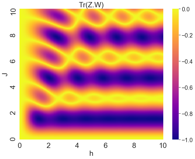
We run our code using the PPT criterion across the parameter space for fixed . As is the time of interaction between the system and the memory, for time the process is trivially Markovian for every nonzero . This is also the case for for every nonzero because the magnetic field is affecting both systems separately. In Appendix A6 and A7 we find all the other parameter values for which the process is Markovian and we prove that for and every nonzero the process is with classical memory (or Markovian).
For a fixed time we run the code for and present our findings in Figure 3. The value becomes negative when the PPT criterion has detected a quantum memory while in all other areas, a value close to zero is in general inconclusive. For this reason, we run the SDP testing the second step of the hierarchy. We find the same results, suggesting that the areas of not detecting a quantum memory were probably areas with classical memory. However, as we present in Appendix A7, the points in the Figure where the lines are crossing correspond to Markovian processes. Additionally, we verify that these are the only Markovian points by calculating the measure of non-Markovianity introduced in Pollock:2018ab, which is the relative entropy Vedral:2002aa between each process with an associated Markovian one Giarmatzi:2018aa. This measure becomes zero when the process is Markovian.
4 Conclusion
We provide a novel approach to the study of non-Markovianity that captures genuine quantum multi-time correlations within a process and allows us to detect an environment with quantum memory without process tomography. Our method expands considerably the investigation of open quantum systems. Our definition of non-Markovianity with classical memory, which leads to mapping entanglement to a quantum memory, provides an experimentally accessible tool and paves the way for further research. It can be used in experimental situations to detect that an external quantum system (environment) retains quantum correlations over time—whether this is desired or not. Furthermore, entanglement leads to many properties for states, which can be mapped to interesting properties for processes, for example multipartite entanglement could correspond to novel types of quantum non-Markovianity in multi-time-step processes. Hence, investigating other properties of entanglement could unveil more information about quantum memory in open quantum systems.
References
- Breuer and Petruccione (2002) H. P. Breuer and F. Petruccione, Oxford University Press, Oxford (2002).
- Arute et al. (2019) F. Arute, K. Arya, R. Babbush et al., Nature 574, 505 (2019).
- Preskill (2018) J. Preskill, Quantum 2, 79 (2018).
- Morris et al. (2019) J. Morris, F. A. Pollock and K. Modi, Non-markovian memory in ibmqx4, (2019), arXiv:1902.07980 [quant-ph].
- Piilo et al. (2008) J. Piilo, S. Maniscalco, K. Härkönen et al., Phys. Rev. Lett. 100, 180402 (2008).
- Wolf and Cirac (2008) M. M. Wolf and J. I. Cirac, Communications in Mathematical Physics 279, 147 (2008).
- Breuer et al. (2009) H.-P. Breuer, E.-M. Laine and J. Piilo, Phys. Rev. Lett. 103, 210401 (2009).
- Rivas et al. (2010) A. Rivas, S. F. Huelga and M. B. Plenio, Phys. Rev. Lett. 105, 050403 (2010).
- Hou et al. (2011) S. C. Hou, X. X. Yi, S. X. Yu et al., Phys. Rev. A 83, 062115 (2011).
- Chruściński and Maniscalco (2014) D. Chruściński and S. Maniscalco, Phys. Rev. Lett. 112, 120404 (2014).
- Rivas et al. (2014) Á. Rivas, S. F. Huelga and M. B. Plenio, Reports on Progress in Physics 77, 094001 (2014).
- Breuer et al. (2016) H.-P. Breuer, E.-M. Laine, J. Piilo et al., Rev. Mod. Phys. 88, 021002 (2016).
- Li et al. (2018) L. Li, M. J. Hall and H. M. Wiseman, Physics Reports 759, 1 (2018).
- de Vega and Alonso (2017) I. de Vega and D. Alonso, Reviews of Modern Physics 89, 015001 (2017).
- Shapiro et al. (1987) J. H. Shapiro, G. Saplakoglu, S.-T. Ho et al., J. Opt. Soc. Am. B 4, 1604 (1987).
- Caves and Milburn (1987) C. M. Caves and G. J. Milburn, Phys. Rev. A 36, 5543 (1987).
- Wiseman and Milburn (1993) H. M. Wiseman and G. J. Milburn, Phys. Rev. Lett. 70, 548 (1993).
- Budini (2001) A. A. Budini, Phys. Rev. A 64, 052110 (2001).
- Zhou et al. (2010) D. Zhou, A. Lang and R. Joynt, Quantum Inf. Process. 9, 727 (2010).
- Bordone et al. (2012) P. Bordone, F. Buscemi and C. Benedetti, Fluctuation Noise Lett. 11, 1242003 (2012).
- Bodor et al. (2013) A. Bodor, L. Diósi, Z. Kallus et al., Phys. Rev. A 87, 052113 (2013).
- Xu et al. (2013) J.-S. Xu, K. Sun, C.-F. Li et al., Nature Communications 4, 2851 (2013).
- Vacchini (2013) B. Vacchini, Phys. Rev. A 87, 030101 (2013).
- Budini (2018) A. A. Budini, Phys. Rev. A 97, 052133 (2018).
- Shaji and Sudarshan (2005) A. Shaji and E. Sudarshan, Physics Letters A 341, 48 (2005).
- Pechukas (1994) P. Pechukas, Phys. Rev. Lett. 73, 1060 (1994).
- Štelmachovič and Bužek (2001) P. Štelmachovič and V. Bužek, Phys. Rev. A 64, 062106 (2001).
- Schmid et al. (2019) D. Schmid, K. Ried and R. W. Spekkens, Phys. Rev. A 100, 022112 (2019).
- Lindblad (1979) G. Lindblad, Comm. Math. Phys. 65, 281 (1979).
- Accardi et al. (1982) L. Accardi, A. Frigerio and J. T. Lewis, Publications of the Research Institute for Mathematical Sciences 18, 97 (1982).
- Chiribella et al. (2009) G. Chiribella, G. M. D’Ariano and P. Perinotti, Phys. Rev. A 80, 022339 (2009).
- Pollock et al. (2018a) F. A. Pollock, C. Rodríguez-Rosario, T. Frauenheim et al., Physical Review A 97, 012127 (2018a).
- Oreshkov et al. (2012) O. Oreshkov, F. Costa and Č. Brukner, Nat. Commun. 3, 1092 (2012), arXiv:1105.4464 [quant-ph].
- Oreshkov and Giarmatzi (2016) O. Oreshkov and C. Giarmatzi, New Journal of Physics 18, 093020 (2016).
- Peres (1996) A. Peres, Physical Review Letters 77, 1413 (1996).
- Doherty et al. (2004) A. C. Doherty, P. A. Parrilo and F. M. Spedalieri, Physical Review A 69, 022308 (2004).
- Nesterov and Nemirovskii (1987) Y. Nesterov and A. Nemirovskii, Interior Point Polynomial Algorithms in Convex Programming, Studies in Applied Mathematics (Society for Industrial and Applied Mathematics, 1987).
- Davies and Lewis (1970) E. Davies and J. Lewis, Comm. Math. Phys. 17, 239 (1970).
- Jamiołkowski (1972) A. Jamiołkowski, Rep. Math. Phys 3, 275 (1972).
- Choi (1975) M.-D. Choi, Linear Algebra Appl. 10, 285 (1975).
- Kretschmann and Werner (2005) D. Kretschmann and R. F. Werner, Phys. Rev. A 72, 062323 (2005).
- Costa and Shrapnel (2016) F. Costa and S. Shrapnel, New Journal of Physics 18, 063032 (2016).
- Giarmatzi and Costa (2018) C. Giarmatzi and F. Costa, npj Quantum Information 4, 17 (2018).
- Pollock et al. (2018b) F. A. Pollock, C. Rodríguez-Rosario, T. Frauenheim et al., Physical Review Letters 120, 040405 (2018b).
- Kołodyński et al. (2020) J. Kołodyński, S. Rana and A. Streltsov, Physical Review A 101, 020303 (2020).
- Chruściński and Maniscalco (2014) D. Chruściński and S. Maniscalco, Physical Review Letters 112, 120404 (2014).
- Araújo et al. (2015) M. Araújo, C. Branciard, F. Costa et al., New J. Phys. 17, 102001 (2015).
- Rains (2019) E. M. Rains, arXiv:9707002 [quant-ph].
- Vedral and Plenio (1998) V. Vedral and M. B. Plenio, Phys. Rev. A 57, 1619 (1998).
- Bennett et al. (1999) C. H. Bennett, D. P. DiVincenzo, C. A. Fuchs et al., Phys. Rev. A 59, 1070 (1999).
- nery2021simple (2021) M. Nery and M. T. Quintino and P. A. Guérin and T. O. Maciel and R. O. Vianna arXiv:2101.11630 [quant-ph].
- Rubino et al. (2017) G. Rubino, L. A. Rozema, A. Feix et al., Science Advances 3 (2017), 10.1126/sciadv.1602589.
- Goswami et al. (2018) K. Goswami, C. Giarmatzi, M. Kewming et al., Phys. Rev. Lett. 121, 090503 (2018).
- Ernst (1925) I. Ernst, Z. Physik 31, 253 (1925).
- Vedral (2002) V. Vedral, Reviews of Modern Physics 74, 197 (2002).
- Milz et al. (2019) S. Milz, M. S. Kim, F. A. Pollock et al., Phys. Rev. Lett. 123, 040401 (2019).
- Milz et al. (2020) S. Milz, F. Sakuldee, F. A. Pollock et al., Quantum 4, 255 (2020).
- Chruściński et al. (2011) D. Chruściński, A. Kossakowski and A. Rivas, Phys. Rev. A 83, 052128 (2011).
- (59) C. Giarmatzi, Github page.
Appendix A Appendix
A.1 Choi representation of processes with classical memory
In this section we provide the definition of a process matrix with classical memory and prove that, as a necessary condition, it is proportional to a separable state.
We consider a finite number of time steps. Each time step is associated with an input and an output space, , , , corresponding to the input and output of an operation that can be performed on the system at time . We use the short-hand . We take the last output space to be trivial, so that . (Equivalently, we could keep a non-trivial final output space , but the constraints defining a causally ordered process—or comb—imply that chiribella09b; Oreshkov12, which means is not relevant for calculating observable probabilities.)
In a quantum process with classical memory, the environment can acquire classical information about the system, which then feeds forwards to influence the system’s evolution at later times. The acquisition of classical information by the environment can be understood as a measurement: during the evolution between times and , the environment measures the system and obtains a classical outcome . The conditional evolution of the system, in general, depends on . Furthermore, the evolution can depend on the information stored by the environment up to that point, which we represent as a classical variable . The most general evolution of this type is represented by a CP map .
If the outcome is discarded, the unconditional evolution of the system between times and is represented by the sum , which must be a CPTP map. In other words, each set of CP maps has to be an instrument. In Choi represenation, an instrument is given by a set of matrices that satisfy
| (1) |
The value of at time can depend on the value of at all previous times, as well as on all the information hitherto extracted from the system, through an arbitrary conditional probability , where we use the short-hand notation (and similarly for ). All the classical information in the environment is eventually discarded, leading to the process matrix
| (2) |
with , . Note that, since we start with an input space, , the “zeroth” instrument reduces to a set of sub-normalised states, , summing up to a normalised state, . This describes an environment that, given the variable , prepares the state with probability .
It can be helpful to give a temporal description of the process (2). Before time , the environment contains some classical variable . Upon measuring the system, the environment obtains a classical outcome . This leaves the system in the (non-normalised) state . At time , the environment’s information is updated to the classical variable , which depends on the previous variables through the conditional probability . Then, between times and , the environment measures the system, obtaining an outcome and resulting in the conditional evolution of the system. The memory at updates to , through , and so on.
We can re-define the CP maps to include the conditional probabilities representing the dependency on past information. Thus we set
| (3) | ||||
| (4) |
where is the marginal probability for the initial variable . It is easy to verify that the newly defined maps form properly normalised instruments:
As now both variables , correspond to measurement outcomes in the instrument, we can further simplify the expression by combining the variables as , . The process matrix now takes the form
| (5) |
As this is a particular form of Eq. (2), we see that a process matrix has classical memory if and only if it can be written in this way. In other words, we can take Eq. (5) as a definition of process with classical memory.
By relabelling , we see that the process matrix (5) is a particular case of the form
| (6) | ||||
where we no longer require that the CP maps sum up to a CPTP map. In other words, the process matrix is proportional to a separable state for the partition , as we set out to prove. Note that this is equivalent to a convex combination of product matrices, as easily seen be redefining , .
We remark that, although all process matrices with classical memory have the form (6), not all matrices of that form are process matrices with classical memory. In other words, it might not be possible to re-write a matrix of the form (6) into the form (5). This is certainly the case for separable states that do not satisfy the constraints for causally ordered process matrices (combs). However, we conjecture that there are combs of the form (6) that cannot be rewritten in the form (5), i.e., that cannot be realised as processes with classical memory.
This conjecture is motivated by the close analogy with “quantum non-locality without entanglement” Bennett1999. In detail, a multi-time process (or comb) defines a multipartite channel from all output to all input spaces, . The process matrix is the Choi representation of . To put this in the context of the relevant literature, we can take to be trivial and . Furthermore, assuming matching dimensions, we identify and . A process matrix of the separable form (6) then corresponds to a channel
| (7) |
where each , is a CP (but not necessarily CPTP) map. A channel of the above form is called separable, in analogy to separable states Rains1997. A subclass is that of LOCC channels, namely channels that can be realised with Local Operations and Classical Communication. For example, an LOCC channel can consist of an instrument performed on system and an instrument on , where depends probabilistically on and (thanks to “classical communication” from to ):
| (8) |
More generally, an LOCC channel can involve the composition of multiple instruments on each side, with multiple rounds of communication between to .
It is relatively simple to see that a channel of the form (8) corresponds to a process with classical memory, according to our definition. The fact that there exist separable channels that do not have an LOCC realisation Bennett1999 strongly suggests that there are combs with the separable form (6) that cannot be realised as processes with classical memory. The only gap is that combs correspond to a strict subset of multipartite channels. Therefore, it is possible that, when adding the comb constraints, separable channels may fall into the LOCC class, and possibly even in the smaller class of processes with classical memory.
A.2 Non-Markovianity witnesses based on dynamical maps
A large body of work on open quantum systems has been concerned with identifying non-Markovian behaviour in dynamical maps, leading to several witnesses and measures of non-Markovianity Rivas2014; Breuer16. Here we compare this approach to our definition of quantum memory and show that common measures of non-Markovianity are not sufficient do decide whether a general process has quantum or classical memory.
A dynamical map is a time-dependent quantum channel, describing the evolution of a system as . The map can be seen as the quantum analogue of a conditional probability distribution for a classical time-dependent stochastic variable . Knowledge of these conditional probabilities does not provide full information about the stochastic process, which is defined through joint probabilities . Similarly, knowledge of the dynamical map does not provide full information about the processes matrix , which encodes arbitrary multipartite correlations Pollock:2018ab.
Nonetheless, one can use dynamical maps to derive sufficient conditions for non-Markovianity. The most commonly used criteria are based on the notion of divisibility Wolf2008. A set of dynamical maps is called divisible if, for any three times , , , the decomposition holds, where all maps are completely positive. Although not all divisible maps correspond to Markovian processes, all Markovian processes give rise to divisible maps Milz2019. Therefore, a failure of divisibility is a signature of non-Markovianty. Our question is whether it is also a signature of quantum memory, as per our definition. Conversely, we also want to know whether a process with classical memory necessarily leads to divisible dynamics. We are going to answer both questions in the negative.
An important observation is that, in the presence of initial correlations between system and environment, dynamical maps are in general not well-defined, as it becomes unclear how to vary the input to the map without specifying the full system-environment state Shaji2005; Pechukas1994; Stelmachovic2001; Schmid2019. This already shows that dynamical maps are unsuitable to study memory in two-time-step scenarios (as our in example in the main text) where non-Markovianity can only arise due to system-environment correlations.
Dynamical maps become well defined in scenarios where the first operation is restricted to be a strong state preparation, removing all initial correlations with the environment (a “causal break” in the language of Refs. Pollock:2018ab; Pollock:2018aa). In this scenario, we can take the input space associated with the first time-step to be trivial, . Non-trivial memory effects can arise when we consider two additional time-steps, and . This leads us to consider process matrices , whose circuit representation is shown in Figure 1. In such a process, the relevant partition to detect quantum memory is .
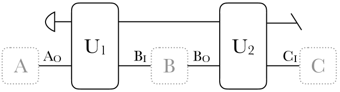
As this process involves three time-steps, we can associate to it three maps: (evolution from to ), ( to ), and ( to ). The relation with the process matrix is as follows (see, e.g., Ref. costa2016; Milz2020kolmogorovextension):
-
1.
is obtained by discarding the last time-step. It is a general property of a quantum comb (causally ordered process matrix) that tracing out the last input space results in the identity matrix on the last output chiribella09b:
(9) is the Choi matrix of the map , and can be obtained directly from the process matrix through
(10) where is the dimension of .
-
2.
is obtained by inserting the identity map as ’s operation. In Choi representation,
(11) Note that, in expressions such as Eq. (11), a re-ordering of subsystem is implied (i.e., appropriate subsystem swaps should be applied to matrices so that subsystems are all in the same order, e.g., the standard order ).
-
3.
is not uniquely specified by , as it depends on the state preparation at . However, in the following we will not need an explicit expression of this map. (In fact, divisibility criteria typically only require the existence of any CP map , not necessarily operationally defined Milz2019).
The first thing we want to prove is that divisibility does not imply classical memory. To this end, we present a process matrix that is entangled across the partition and whose associated maps satisfy divisibility. The example is
| (12) | ||||
| (13) |
with the notation . This process can be realised through the circuit in Fig. 2. As the “GHZ state” is entangled across any bipartition, it is clear that this process matrix has a quantum memory. A simple calculation reveals the Choi matrices of the relevant maps to be
| (14) | ||||
| (15) |
Thus, the two maps are equal, each describing a dephasing channel . These maps are clearly compatible with divisible dynamics. In particular, the criterion in Ref. Rivas10 states that evolution is divisible if and only if the probability of success in a one-shot state discrimination task cannot increase. This is clearly true in our example: for any given state preparation at time , tomography at would reveal the same state as at time . Memory signatures in process (12) are encoded in genuinely tripartite correlations across . Hence, divisibility does not imply classical memory.
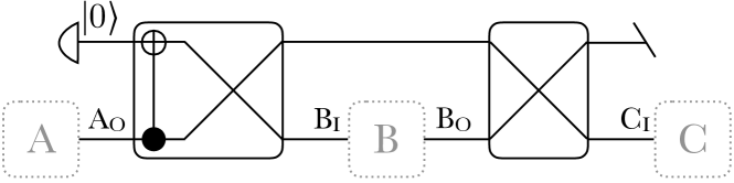
Let us now show that non-divisibility does not imply quantum memory. We will present a process with classical memory and show that its associated maps are non-divisible. To this end, for divisibility, it is sufficient to consider the criterion proposed in Ref. Breuer09: given two initial states , , prepared at , their trace distance cannot increase under divisible dynamics; the trace distance is defined as , . We want to present a process with classical memory that increases the trace distance of two states, implying non-divisibility. The example is
| (16) |
with an arbitrary density matrix. This process has the form (5) and thus can be realised with classical memory, through the circuit in Figure 3. Explicitly, between the first and second time step ( to ) the environment measures the system in the computational basis, yielding outcome , and prepares the unrelated state . Between second and third step ( to ), the system’s state is discarded and the pure state is prepared, which only requires the environment to keep memory of the classical output from the first time step. This results in a dephasing channel from the first to the third step ( to ). Now, consider states , prepared at . Their trace distance drops to at , as any state is replaced by . However, at the initial value is restored, , as both states are mapped identically from to . Hence, a process with classical memory can involve non-divisible maps, which means that non-divisibility does not imply a quantum memory.
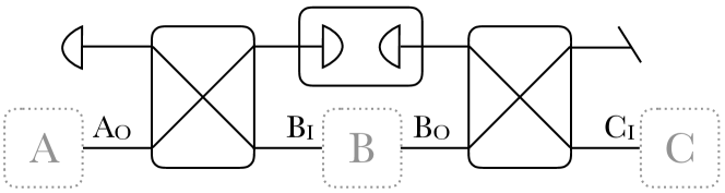
This example is not surprising, as it is known that the (classical analogue of the) trace-distance criterion is violated by classical stochastic processes Chruscinski2011, and thus it is fully expected that it can be violated by quantum processes with classical memory.
A.3 Initial system-environment correlations affecting the memory
In this section we discuss what happens to a general 2-time-step scenario (one system-environment interaction), with initial system-environment correlations, described in the initial joint state , where denotes the environment state space at the initial time. The process matrix is obtained using the rules to construct quantum combs, by sequential composition of processes chiribella09b. We start with the initial state and the joint unitary in the form of its Choi matrix , and combining them using the link product, defined as
| (17) |
where the superscript on the subsystem denotes partial transposition with respect to the subsystem.
A.3.1 Case 1: is a product state
In this case , with and being arbitrary states. The process matrix becomes
| (18) |
where is the channel for the system after tracing out the environment. We see that this is the form of a Markovian process matrix.
A.3.2 Case 2: is a separable state
In this case, , with , , and . Now the process matrix becomes
| (19) |
where, ,
represents a CPTP map. We see that, for , Eq. (19) has the form of a process with classical memory, Eq. (5).
We conclude from the above that for a two-time-step process, and any kind of system-environment interaction, there can be no quantum memory in the environment if there is no initial entanglement between the environment and the system.
A.4 Process matrix of our example
For the process matrix for our example we start with the one written above for the general two-time-step process
| (20) |
with the partial transpose acting on the common subsystem that is traced over. We then substitute and, omitting the tensor product symbols,
| (21) |
while the initial state is , so that . The link product then gives
| (22) |
which is, up to normalisation, the same expression as (21), with the first two factors swapped and substituted with . The process matrix describing the first qubit is obtained by tracing out .
A.5 SDP: Higher-order criteria
For the second level of the hierarchy, the problem is no longer a simple computational task—we need to find if there exist a symmetric extension of a state (corresponding to a process matrix ), such the state and all its partial transposes with respect to and are positive. The latter conditions are linear constraints on and so the problem can be cast as an SemiDefinite Program which can be solved efficiently Doherty:2004aa. We develop this method as it is a stronger test of non-separability, although in our example it turns out that the first level completely characterizes the type of non-Markovinity.
An SDP has a primal and a dual form. The primal form is written as
| variable | |||||
| minimize | |||||
| subject to | (23) |
where c is a known vector, and , for some fixed hermitian matrices , is a semidefinite matrix. In the case where there is no function to minimise and the problem reduces to whether the constraints are satisfied for some value of . This is called the feasibility problem. Its associated dual form is written as
| variable | |||||
| maximize | |||||
| subject to | (24) | ||||
In our case, the feasibility problem is formulated as follows
| variable | |||||
| minimize | |||||
| subject to | (25) | ||||
where we have omitted the spaces the states live on, and . This SDP tries to find an extension of , , such that it is separable according to the PPT criterion. is constrained to be an extension of with the last two constraints and that it is a positive semidefinite matrix. Note that a block diagonal matrix is non-negative if and only if each of its block matrices is non-negative.
The primal SDP detects entanglement when its output is that the problem is infeasible, i.e. it cannot find an extension of such that it is separable according to the PPT criterion. The dual SDP minimises a value to find a witness for ; from which we find a witness for . To explicitly write the dual form we need some definitions. Due to symmetries on the extension , it can be written as follows
| (26) |
where is a fixed part that depends only on the given and is the coefficients for the rest of the basis elements . In particular, , and is a linear map from to . If we then define we get that and .
The dual form of the SDP then writes
| variable | |||||
| maximize | |||||
| subject to | (27) | ||||
For a positive value of , which yields a negative one for , we can obtain a witness for through , where is the adjoint map of . The codes for the feasibility and dual problem for our example are publicly available on GitHub sdps.
A.6 Our example: classical memory in the case
In this case the Hamiltonian is
| (28) |
so it has product eigenstates, built from the Pauli matrix’s eigenstates , :
| (29) | ||||
| (30) | ||||
Using the eigenstates of in the definition of the Choi isomorphism, and taking the partial trace over of expression (22), we obtain for the process matrix
We see that this matrix is an equal mixture of two product matrices:
Therefore, the process we are describing is the equal mixture of two Markovian processes: for respectively, these correspond to processes where the system is initially in state , while from to it evolves according to the (single-qubit) Hamiltonian . Thus, even though in our model the initial system-environment state is entangled, the process for the system alone can be reproduced by substituting the environment with a classical variable, which samples with equal probabilities the values , and determines both the initial state and the evolution from first to second time-step.
A.7 Our example: markovian points
Here we find the parameters , , for which the process is Markovian. A sufficient condition is that the unitary matrix that represents the system-environment evolution factorises: . As , it is sufficient to consider the case.
We find that the unitary factorises for the parameter values
plus an additional point , for which .
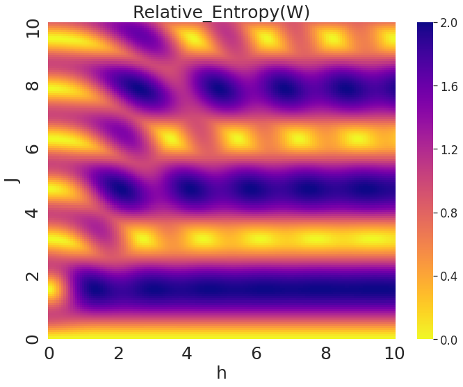
In principle, there could be parameter values for which the evolution is not trivial but the process is Markovian. We verified that this is not the case numerically: for a range of parameters, we calculated the relative entropy Pollock:2018ab; Vedral:2002aa between and the corresponding Markovian process , where and are obtained as partial traces of . The relative entropy between two states and is . Note that our states corresponding to process matrices are non-normalised, so we used and .
We found that the relative entropy vanishes (and hence the process is Markovian) only for the parameter values found above. The values of the relative entropy are shown in Figure 4.
References
- Chiribella et al. (2009) G. Chiribella, G. M. D’Ariano and P. Perinotti, Phys. Rev. A 80, 022339 (2009).
- Oreshkov et al. (2012) O. Oreshkov, F. Costa and Č. Brukner, Nat. Commun. 3, 1092 (2012), arXiv:1105.4464 [quant-ph].
- Bennett et al. (1999) C. H. Bennett, D. P. DiVincenzo, C. A. Fuchs et al., Phys. Rev. A 59, 1070 (1999).
- Rains (2019) E. M. Rains, arXiv:9707002 [quant-ph].
- Rivas et al. (2014) Á. Rivas, S. F. Huelga and M. B. Plenio, Reports on Progress in Physics 77, 094001 (2014).
- Breuer et al. (2016) H.-P. Breuer, E.-M. Laine, J. Piilo et al., Rev. Mod. Phys. 88, 021002 (2016).
- Pollock et al. (2018a) F. A. Pollock, C. Rodríguez-Rosario, T. Frauenheim et al., Physical Review Letters 120, 040405 (2018a).
- Wolf and Cirac (2008) M. M. Wolf and J. I. Cirac, Communications in Mathematical Physics 279, 147 (2008).
- Milz et al. (2019) S. Milz, M. S. Kim, F. A. Pollock et al., Phys. Rev. Lett. 123, 040401 (2019).
- Shaji and Sudarshan (2005) A. Shaji and E. Sudarshan, Physics Letters A 341, 48 (2005).
- Pechukas (1994) P. Pechukas, Phys. Rev. Lett. 73, 1060 (1994).
- Štelmachovič and Bužek (2001) P. Štelmachovič and V. Bužek, Phys. Rev. A 64, 062106 (2001).
- Schmid et al. (2019) D. Schmid, K. Ried and R. W. Spekkens, Phys. Rev. A 100, 022112 (2019).
- Pollock et al. (2018b) F. A. Pollock, C. Rodríguez-Rosario, T. Frauenheim et al., Physical Review A 97, 012127 (2018b).
- Costa and Shrapnel (2016) F. Costa and S. Shrapnel, New Journal of Physics 18, 063032 (2016).
- Milz et al. (2020) S. Milz, F. Sakuldee, F. A. Pollock et al., Quantum 4, 255 (2020).
- Rivas et al. (2010) A. Rivas, S. F. Huelga and M. B. Plenio, Phys. Rev. Lett. 105, 050403 (2010).
- Breuer et al. (2009) H.-P. Breuer, E.-M. Laine and J. Piilo, Phys. Rev. Lett. 103, 210401 (2009).
- Chruściński et al. (2011) D. Chruściński, A. Kossakowski and A. Rivas, Phys. Rev. A 83, 052128 (2011).
- Doherty et al. (2004) A. C. Doherty, P. A. Parrilo and F. M. Spedalieri, Physical Review A 69, 022308 (2004).
- (21) C. Giarmatzi, Github page.
- Vedral (2002) V. Vedral, Reviews of Modern Physics 74, 197 (2002).
