Deep Learning Applied to the Asteroseismic Modeling of Stars with Coherent Oscillation Modes
Abstract
We develop a novel method based on machine learning principles to achieve optimal initiation of CPU-intensive computations for forward asteroseismic modeling in a multi-D parameter space. A deep neural network is trained on a precomputed asteroseismology grid containing about 62 million coherent oscillation-mode frequencies derived from stellar evolution models. These models are representative of the core-hydrogen burning stage of intermediate-mass and high-mass stars. The evolution models constitute a 6D parameter space and their predicted low-degree pressure- and gravity-mode oscillations are scanned, using a genetic algorithm. A software pipeline is created to find the best fitting stellar parameters for a given set of observed oscillation frequencies. The proposed method finds the optimal regions in the 6D parameters space in less than a minute, hence providing the optimal starting point for further and more detailed forward asteroseismic modeling in a high-dimensional context. We test and apply the method to seven pulsating stars that were previously modeled asteroseismically by classical grid-based forward modeling based on a statistic and obtain good agreement with past results. Our deep learning methodology opens up the application of asteroseismic modeling in +6D parameter space for thousands of stars pulsating in coherent modes with long lifetimes observed by the Kepler space telescope and to be discovered with the TESS and PLATO space missions, while applications so far were done star-by-star for only a handful of cases. Our method is open source and can be used by anyone freely111The source code to run the analysis can be found at https://github.com/l-hendriks/asteroseismology-dnn.
1 Introduction
The past decade has seen tremendous progress in stellar physics, largely thanks to the application of asteroseismology (Aerts et al., 2010). Such applications are nowadays based on long-term uninterrupted space photometry with a precision of mag assembled for thousands of stars by the European CoRoT (Auvergne et al., 2009) and the NASA Kepler (Koch et al., 2010) space telescopes. This data offers the opportunity to confront stellar evolution theory with asteroseismic data probing the stellar interior, rather than with spectroscopic data giving information on the stellar surface.
Comparison between asteroseismic data and stellar models is done by computing the spectrum of oscillation modes predicted by the theoretical models. Oscillation modes are called pressure modes or gravity modes, depending on whether the pressure force, respectively buoyancy, is the dominant restoring force. Pressure modes probe the physical conditions in the stellar envelope while gravity modes tune the deep stellar interior. A modern educational tutorial containing various statistical methods for asteroseismology is available in Appourchaux (2014).
Statistical inference in asteroseismology can conveniently be done from forward modeling. Usually, one adopts a grid-based approach and considers millions of stellar structure models of different evolutionary stage. Applications to low-mass stars in the core hydrogen burning stage can be found in the pioneering papers by Miglio & Montalbán (2005) and Quirion et al. (2010), while Brassard et al. (2001) developed methodology to treat coherent gravity modes in core helium burning subdwarf stars. In the past few years, forward modeling based on space asteroseismology has been focused strongly on solar-like oscillations in low-mass stars because the Kepler mission provided data for thousands such objects. Their damped pressure modes are stochastically excited by the turbulent convection in their outer convective envelope and have periodicities ranging from minutes for the core hydrogen burning phase to hours for red giants. The forward modeling for such “sun-like” stars relies on stellar models whose input physics is taken to be very similar to the one of solar models calibrated from helioseismology. Such applications are nowadays often based on Bayesian statistics, e.g. as in Appourchaux et al. (2012); Gruberbauer et al. (2013); Corsaro & De Ridder (2014); Davies et al. (2016); Deheuvels et al. (2016); Silva Aguirre et al. (2017), among others.
A prominent application of Machine Learning (ML) applied to low-mass star asteroseismology based on damped pressure modes was developed by Bellinger et al. (2016). It is based on the combined use of spectroscopic and asteroseismic input and relies on the principle of random forests. This application covers the mass range M⊙ and delivers parameter estimation in a 7D space: stellar mass, age, initial helium, initial metalicity, mixing length value, convective overshoot, and an amplification factor for atomic diffusion (excluding radiative levitation, i.e., focusing only on the settling of elements heavier than hydrogen). The metalicity and effective temperature were found to be the two dominant features feeding the ML code. These turn out to be about a factor three higher in feature importance than the seismic large and small frequency separations and frequency ratios.
The situation is totally different in our application to stars of higher mass. The required spectroscopic input is not available at sufficiently high precision for those. Moreover, one cannot use scaled versions of solar physics because ingredients that do not occur in low-mass stars dominate for intermediate- and high-mass stars. In particular, the initial helium content and settling of heavy elements play inferior roles compared to core overshooting and macroscopic chemical mixing due to various phenomena like rotation and waves in the radiative envelope. From a seismic point of view, intermediate- and high-mass stars born with a convective core and a radiative envelope (M⊙) reveal coherent modes with long lifetimes, rather than damped modes in low-mass stars. The frequencies of coherent modes can be fitted directly, because they are not subject to uncertain physics in the stellar atmosphere as occurs for damped modes triggered by envelope convection. Due to these differences in the treatment of the theory of stellar structure and of stellar oscillations for the different mass regimes, their asteroseismic modeling requires different approaches. Aerts et al. (2018, hereafter termed Paper I) provided an extensive discussion on the physical and pulsational ingredients that are dominant for asteroseismic modeling of stars born with a convective core. Applications in the recent literature (Kurtz et al., 2014; Saio et al., 2015; Moravveji et al., 2015, 2016; Murphy et al., 2016; Schmid & Aerts, 2016; Van Reeth et al., 2016; Sowicka et al., 2017; Kallinger et al., 2017; Szewczuk & Daszyńska-Daszkiewicz, 2018) were done at a very different level of detail compared to low-mass pulsators and, with the exception of Johnston et al. (2018), none so far achieved error estimation taking into account parameter correlations and the fact that the stellar models depend nonlinearly on the parameters.
The mass of core hydrogen burning stars with detected coherent modes ranges roughly from 2 to 30 solar masses. For such stars, the physics of the near-core region is largely unknown. Moreover, mass loss due to a radiation-driven wind is active as of stellar birth for masses above M⊙ and for those a high binary rate occurs. One therefore faces tremendous challenges in the forward modeling of these stars in terms of dimensionality and CPU requirements compared to the “easy” case of low-mass sun-like pulsators. On the other hand, their coherent modes, and in particular gravity modes, probe the deepest layers of those stars with high precision, rather than just the envelope as damped pressure modes in low-mass stars. It has been shown that this property offers the opportunity to test the near-core physics (Pedersen et al., 2018). Gravity-mode asteroseismology opens up the possibility to derive the helium core mass near the end of the core hydrogen burning stage from such modes, a prominent quantity that lays the foundation for the further evolution of the star in terms of nuclear yields.
The current theory of angular momentum transport fails to explain asteroseismic data by more than an order of magnitude (see Aerts et al., 2019, for an extensive review of the current status of interior rotation rates of more than a thousand stars). This theory can be improved from gravity-mode asteroseismology by applying the method in Paper I. Similarly, the theory of element transport can now be calibrated asteroseismically (see Salaris & Cassisi, 2017, for a review). The potential gain from asteroseismology of high-mass stars is thus much larger than for low-mass stars in terms of chemical enrichment of the galaxy.
Here, we focus on intermediate- and high-mass core hydrogen burning stars in the mass range M⊙ with detected coherent oscillation modes. Our aim is to develop and provide an optimal deep learning tool as a critical start-up ingredient for efficient forward asteroseismic modeling in a +6D parameter space. In particular, we wish to explore the performance of a deep learning network in order to gain computational efforts, because the “manual” asteroseismic modeling applied to a few stars with coherent modes so far required months of analysis work, with a high risk of missing local minima in parameter space (cf. Ausseloos et al., 2004, for an example of such a systematic efforts). This is not practical for future applications to samples of tens to hundreds of stars anticipated by future space missions, such as TESS (Ricker et al., 2016) and PLATO (Rauer et al., 2014). In this paper, we restrict to slowly-rotating pulsators. Future work will consider deep learning methods for asteroseismology of fast rotators.
2 Stellar Models and Their Coherent Oscillations
Aside from other variability features, a large fraction of the core-hydrogen burning intermediate-mass and high-mass stars reveal so-called coherent modes. In contrast to the damped oscillation modes of low-mass stars, these coherent modes are self-driven by a heat mechanism and have long lifetimes of thousands to millions of years (e.g., Aerts et al., 2010, Chapter 2). This implies that these modes are easily detectable in high-precision uninterrupted long-duration time-series data, provided that they are excited with amplitudes above the detection threshold of the instrument. The time base of such data is crucial because, unlike the short periods of the damped oscillations of low-mass stars, the coherent modes we are dealing with here have periods from about an hour up to several days, leading to years-long beating patterns to be covered with data. This is particularly the case for gravity-mode oscillations, which probe the deep stellar interior. As such, the 4-year nominal Kepler mission provides the best observations to analyze the period-spacing patterns expected for such modes from theory (Miglio et al., 2008; Bouabid et al., 2013) and actually detected in data (e.g., Van Reeth et al., 2015; Bowman, 2017; Pápics et al., 2017, and references therein). Indeed, while the discovery of period-spacing patterns of gravity modes could be achieved from the 150-day light curves assembled with CoRoT (Degroote et al., 2010; Pápics et al., 2012), this time base was too short to unravel all the beating patterns between the modes and to identify them in terms of their degree and azimuthal order .
The 4-year long monitoring from space by Kepler revealed suitable data sets to detect and identify the degree and radial order, , of several to tens of coherent gravity modes, opening up the opportunity of forward asteroseismic modeling of such modes. As said, we focus on stars born with a convective core and a radiative envelope, in the core hydrogen burning phase of their evolution (the so-called main sequence). The aim of their forward asteroseismic modeling is to fit their detected and identified oscillation frequencies () with values predicted theoretically from stellar models and to evaluate in this way the free parameters that are required as input to compute the stellar interior properties adopted in these models.
A multitude of unknowns for the input physics occurs in stellar models of massive stars, even when fixing the microphysics (Aerts et al., 2018). Many of these unknowns in the macrophysics must be assigned constant values for computational reasons. Moravveji et al. (2015) determined a hierarchy of importance for asteroseismic modeling and showed that the two dominant uncalibrated ingredients in the models are core overshooting and envelope mixing. Their relevant profiles, and (in the notation of Paper I), remain unknown. Because the bare minimum of stellar modeling in terms of input parameters is 4D without consideration of core overshooting and envelope mixing, asteroseismic modeling of massive stars is done by evaluating the average level of these two most important phenomena, rather than their shape. As such, and are simplified to two free parameters to estimate, denoted here as and . This lies at the basis of asteroseismic model grids for intermediate- and high-mass star asteroseismology. Only after having achieved estimation of the average levels of and for sufficient pulsators can one move on to more sophisticated estimation of their profiles to assess theoretical concepts such as rotational mixing, wave transport, etc. Aerts et al. (2019) provides an extensive discussion of such phenomena and how asteroseismology is being used to tune them.
In this work, we relied on a 6D grid of stellar evolution models, covering a wide range in stellar mass from 2 to 20 M⊙. This grid was constructed in the framework of the European FP 7 SpaceInn Project.222This grid is publicly available from fys.kuleuven.be/ster/Software/grid-massive-stars It has been computed with the open-source code MESA (see the MESA instrument papers by Paxton et al., 2011, 2013, 2015, 2018, for extensive documentation). The grid is based on the same input physics as used and described by Schmid & Aerts (2016); the MESA inlist is provided in that paper and therefore omitted here to avoid repetition.333Electronic versions of the MESA and GYRE inlists that lie at the definition of this grid can be retrieved from the MESA Marketplace: http://cococubed.asu.edu/mesa-market/ In brief, the models are based on the following input physics: solar metal mixture by Asplund et al. (2009), OPAL opacity tables by Iglesias & Rogers (1996), mixing-length theory of convection with a fixed mixing-length parameter of 1.8 (expressed in local pressure scale heights), and the Schwarzschild criterion for convective stability.
This SpaceInn grid contains 352 800 models of non-rotating stars following the arguments of such an approach for asteroseismic modeling outlined in detail in Aerts et al. (2018) and in Aerts et al. (2019). The grid covers the evolutionary phase from the zero-age main sequence (ZAMS) until depletion of central hydrogen at the terminal-age main sequence (TAMS), in steps of 0.01 in central hydrogen mass fraction . Different chemical compositions in terms of initial mass fractions were considered: initial hydrogen mass fractions of 0.68, 0.70, and 0.72, and initial metalicities ranging from 0.012 to 0.020 in steps of 0.002. The models were computed for exponential core overshooting in the description by Herwig (2000) and parametrized by a single parameter (expressed in local pressure scale heights), ranging from 0.00 to 0.05, in steps of 0.01 (we refer to Paxton et al. (2011) for details of its implementation in MESA). Given that all asteroseismic modeling results of intermediate-mass stars based on Kepler data demanded “extra” mixing in the radiative envelope to comply with the detected trapping of gravity-mode oscillations in the near-core region, in addition to core overshooting (e.g., Moravveji et al., 2015, 2016; Schmid & Aerts, 2016), the four levels of constant envelope chemical mixing that were required so far for Kepler pulsators were considered, i.e., cm2 s-1. This implies that the SpaceInn grid is a 6D stellar model grid with parameters , .
For chosen time steps along the evolutionary track, or equivalently values, the equilibrium models are perturbed in a linear framework to compute oscillation modes and their accompanying frequencies. Here, we limit to frequencies of coherent low-degree () zonal () gravity and pressure modes, computed for each of the values of between the ZAMS and the TAMS. These oscillation modes were computed with the public code GYRE (Townsend & Teitler, 2013; Townsend et al., 2018), adopting the Cowling and adiabatic approximations as a good approach, as argued in Aerts et al. (2018). We considered radial modes (degree ) and non-radial modes of degree , for radial orders , covering a range in frequencies (in an inertial frame) of roughly d-1. In this way, we have about 62 million oscillation-mode frequencies available in the model grid.
Johnston et al. (2018) and Mombarg et al. (in preparation) provide thorough discussions on how to treat parameter choices, their degeneracies, and their (often modest) deviation from linearity with respect to the stellar model properties. These two papers also discuss the way forward to deal with uncertainties following the statistical framework in Aerts et al. (2018), building on earlier assessments of parameter correlations by Ausseloos et al. (2004), Pápics et al. (2014), and Moravveji et al. (2015). Manual forward modeling to estimate and so far ignored parameter correlations in the error estimation, also for low-mass stars with damped modes (Deheuvels et al., 2016). As discussed at length in Johnston et al. (2018), this is also the case in any binary modeling so far. The DNN provided here is a first step to improve upon manual analyses in terms of computational cost; it will need future upgrades to deal with correlations among the parameters and to deliver appropriate error estimation in a Bayesian framework, just as the manual analyses.
3 Forward Asteroseismic Modeling of Coherent Oscillation Modes
Aerts et al. (2018) outlined in extensive detail the principles of forward asteroseismic modeling of coherent oscillation modes in the mass regime we consider here. In that work, the authors provided a statistical methodological framework for such modeling, taking into account that these oscillation modes depend non-linearly on the free parameters of stellar models and that these parameters are correlated. Their method is based on Maximum Likelihood Estimation (MLE) and statistical model selection. We refer to that paper for details, but repeat here that such modeling requires initial screening of a large grid of stellar models in at least a 7D parameter space when dealing with oscillations in rotating stars. For slow rotators, as we treat here, one dimension can be avoided as one does not need to estimate the rotation frequency of the star whenever it is so slow that rotation and the accompanying Coriolis and centrifugal forces can be ignored in the pulsational computations. In that case, one can reduce to the 6D parameter space as outlined for the SpaceInn model grid in the previous section.
The method in Paper I requires the computation of various refined stellar model grids, with different values for the input physics, in order to find a good match between the observed oscillation frequencies and the theoretically predicted frequencies, to within the measurement errors. The latter are typically smaller than 0.001 d-1, such that the step sizes for , are required to be much smaller than in the SpaceInn grid (e.g. Moravveji et al., 2015, for the first very detailed study and application). This procedure is only manageable (CPU-wise) to apply to ensembles of stars when appropriate “initial” values for at least a few of the six parameters can be achieved, such that the computation of refined grids can be limited to appropriate sub-spaces of the , parameter space. Here, we develop a deep learning method to achieve such an optimal initial guess, as an ideal starting point to apply the methods in Paper I.
A major difference with the ML method developed by Bellinger et al. (2016), which was discussed above, is that the observables we rely on as input for the machine learning only constitute of asteroseismic quantities in the case of the intermediate- and high-mass stars considered here. Indeed, unlike for the low-mass sun-like stars, we do not have high-precision spectroscopic estimates of the gravity , effective temperature and metalicity that can compete with the asteroseismic data. For nominal Kepler data, the coherent modes have frequency errors at the level of , while the relative precisions for , and surface abundances from spectroscopy of stars in the mass range considered here are typically above 10% (e.g. Morel et al., 2006, 2008; Martins et al., 2012b, a; Van Reeth et al., 2015). So there is at least two orders of magnitude difference in the quality of the spectroscopic and asteroseismic information (see Table 1 in Aerts et al., 2019, for a detailed discussion on this matter). Moreover, coherent modes in stars with a convective core and a radiative envelope do not fulfil frequency separations as for high-frequency damped pressure modes. Hence, we cannot rely on scaling relations to estimate the mass and radius as is the case for solar-like oscillations. In this respect, our set-up and application is quite different from the case of low-mass stars with damped pressure modes as in, e.g., Appourchaux et al. (2012); Gruberbauer et al. (2013); Corsaro & De Ridder (2014); Davies et al. (2016); Bellinger et al. (2016); Silva Aguirre et al. (2017), among others.
Whenever spectroscopic, interferometric or astrometric data at level of precision of the oscillation frequencies would become available in the future, they can of course be included in future asteroseismic modeling applications. However, our setup here only relies on the oscillation frequencies and (partial) identification of the mode degree and radial order belonging to every measured oscillation frequency . The challenge is that we treat a mass range that is very large compared to applications done so far: M⊙. We test in how far a deep neural network manages (or not) to pinpoint an appropriate narrow mass and age range from such a large spread in stellar parameters, from just a few (partially) identified oscillation mode frequencies without any other observational input.
4 Deep Neural Networks
Neural networks, and deep neural networks (DNNs) in particular, have received a lot of attention recently, mainly because of the advancements in computer vision and natural language processing. Although the theory behind neural networks is quite old, only now are the datasets sufficiently large and the required processing power good enough to attain high accuracies on many different types of computational problems. In this work, a DNN is trained on an asteroseismological grid of intermediate-mass and high-mass stars to predict the frequencies of their coherent oscillation modes. This is a typical regression problem.
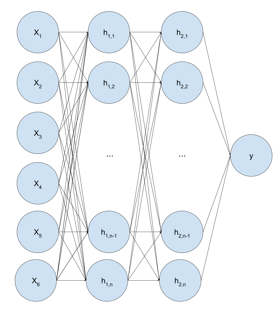
The neural network architecture used in this work is a fully connected or dense network. A schematic view of a dense network is shown in Fig. 1. The input vector in this example is 6-dimensional and the output is 1-dimensional. In between are two layers that are -dimensional. The layers have 6, , and 1 neurons, respectively, in this case. The value of each neuron, except the input neurons, is determined by the following function:
| (1) |
where is called the activation function, is a weight parameter between two neurons (the arrows in Fig. 1) and is a bias term. In order to add non-linearities to the neural network, the activation function must be non-linear. A typical choice is the Rectified Linear Unit (ReLU, Nair & Hinton, 2010). This function is defined as if and if .
By starting from the input layer and calculating all values of all neurons layer-by-layer, the output is finally computed. Initially, the weights and biases are set to random numbers and during training the weights are adjusted to correctly predict a predetermined training set. To validate that the network has correctly learned to predict the occurring features, the network is evaluated on a separate validation set. Typically, the validation set is 10% to 20% of the total dataset. For regression problems, this typically is a mean-squared error between the prediction by the neural network and the actual output belonging to a particular training sample. By backpropagating the error through the network, the weights and biases are updated to improve the cost function in the next iteration (Chauvin & Rumelhart, 1995).
A typical caveat of training neural networks is overfitting. This means the neural network learns to replicate the exact results of the training set, instead of generalizing over the particular samples and learning the underlying correlations. This can be solved by adding a penalty term for high-valued weights, which is called regularization (Ng, 2004). One can verify if a network is overfitted by comparing the training and validation set accuracy. If the training loss is decreasing but the validation loss is increasing, the network is overfitting. A more thorough introduction into deep learning and the validation approach we followed here is given in the Appendix of Caron et al. (2018), to which we refer for further details.
5 Deep neural networks applied to asteroseismic modeling
The aim of this work is to train a neural network that is able to predict the frequencies of the coherent pulsation modes of a given star with detected oscillation frequencies belonging to identified modes . We want to achieve the capacity to quickly search the parameter space spanned by the stellar parameters to find the optimal values for given measurements of the oscillations, without relying on any other information.
The choice of using deep neural networks for this problem has several reasons. Firstly, the size of the dataset is quite large. From the grid, around 62 million oscillation modes are extracted and the objective is to predict the frequency belonging to specific modes given by a wide range of stellar parameters. The aim is not to train on parameters of a particular star, but for all possible stellar parameters that are available in the dataset in one go. This forces the machine learning algorithm to generalize over all parameters and learn the underlying structure. It also means that the network only has to be trained once, and then can be applied to all stars that reside somewhere inside the training grid. Although training can take some time (around 6 hours for this work), evaluation is typically very fast (for this work in the order of microseconds per inference) and the network size is not very large (the compressed network file of this work is 370MB). Furthermore, by adding a batch normalization layer as the first layer inside the network, the issue of incorrectly weighting parameters as stated in Bellinger et al. (2016) is no longer present. The normalizing layer normalizes all data before it is fed to the trainable parameters.
In Bellinger et al. (2016) it is also stated that deep learning based regression is unconstrained. In this work that is indeed the case. However if the network accuracy is high enough this does not have to be a problem. If it would be a problem, it is trivial to design a constrained activation function that is bounded between two values. For example the hyperbolic tangent activation function is bounded between and can trivially be scaled and translated to get a bound between two values. A downside of deep learning compared to random forests is that it is fairly easy with random forests to get insights into why particular predictions are being made, while this information is not accessible from a deep neural network. Training a deep network is also typically more difficult due to the high number of hyperparameters that need to be set correctly to optimally train on the data.
| Layer # | Layer type | Number of neurons |
|---|---|---|
| 1 | Input layer | 8 |
| 2 | Batch normalization | |
| 3 | Fully connected | 500 |
| 4 | Fully connected | 500 |
| 5 | Fully connected | 500 |
| 6 | Fully connected | 500 |
| 7 | Fully connected | 500 |
| 8 | Fully connected | 500 |
| 9 | Fully connected | 5000 |
| 10 | Fully connected | 5000 |
| 11 | Fully connected (tanh) | 5000 |
| 12 | Fully connected (linear) | 1 |
In this work, a DNN is trained using TensorFlow (Abadi et al., 2015) and TFLearn (Damien et al., 2016) on an asteroseismic grid of intermediate- and high-mass stars to predict the frequencies of their coherent oscillation modes. The neural network architecture is shown in Table 1, which has a total number of 53,777,033 trainable parameters. Different neural network architectures have been evaluated and the architecture described in Table 1 provided the best accuracy. In addition, different hyperparameter combinations have been evaluated. The network is trained using the Adam optimizer (Kingma & Ba, 2014) with a learning rate of and a batch size of 2048.
The input data for the neural network is 8D: the six stellar parameters (, , , , , and ) and two integer mode quantum numbers connected with the frequency of the zonal mode: and . The output of the network is the mode frequency for all modes with degree 0, 1, or 2 and for all radial orders (cf. Fig. 1).
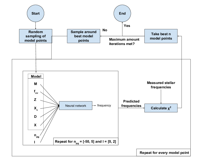
A typical asteroseismic measurement consists of a list of frequencies with corresponding and values. Often, the and -values are not (all) known, but can be one of several values or depend on the values for (one of) the other frequencies. For example , where is the -th value corresponding to a particular frequency. As the neural network predicts one frequency from a list of stellar parameters and a combination of and , another method is needed to find the optimal combination of and values, given a measurement of multiple frequencies. The method used in this work is a genetic algorithm that tries to find the best fit values for a given list of observed frequencies. For every combination of the six stellar parameters, all frequencies are calculated for and between and in one batch. On an Nvidia GTX1080, these 168 evaluations take about 6 milliseconds. Then, the best fitting combination of and values are chosen following a cost function specified below. The cost is minimized using a particle filter, which follows the same procedure as in Achterberg et al. (2015):
-
1.
Start with a random sample of points;
-
2.
Take the points with the least error (lowest cost);
-
3.
Sample points around the points taken from the previous step, using a Gaussian prior with as mean the parameter values and standard deviation times the mean;
-
4.
Repeat steps 2 and 3 times;
-
5.
Repeat steps 2, 3 and 4 also with a standard deviation of and times the mean.
The cost function mentioned above is different than the cost function of the neural network. In this step, the neural network is already trained and not optimized anymore. In addition, the loss of the neural network is not propagated to the cost function of the particle filter. This is because the error of the neural network is constant over all predictions. In a future update the neural network output will also contain uncertainty information (see Section 7). The cost function that is to be minimized is one of the following options, depending on how much is known about the measured oscillation frequencies:
-
1.
If a list of frequencies with exactly known and values is available, those values are compared to the predicted values. The cost of the predicted point with respect to the measurement is , where represents predicted frequencies and measured frequencies, following the notation of Paper I.
-
2.
If for a list of frequencies is available, but can be one of multiple values, all possible values are tested and the minimum error is used in the same cost function as the previous item.
-
3.
If for a list of frequencies only is known that the frequencies are decreasing for decreasing , the best fitting value is used in the list of possible values, bounded by or different bounds if known.
-
4.
If for a list of frequencies only their relative differences are known, the as defined in the first item is calculated for every possible combination of and values within the bounds or different bounds if known.
The analysis setup above defines a recipe to find the best fit star parameters in a straightforward way:
-
1.
Given a measurement, define the cost function set up given by the above possibilities;
-
2.
Using this cost function, find the best stellar parameters using a particle filter that evaluates on the network output.
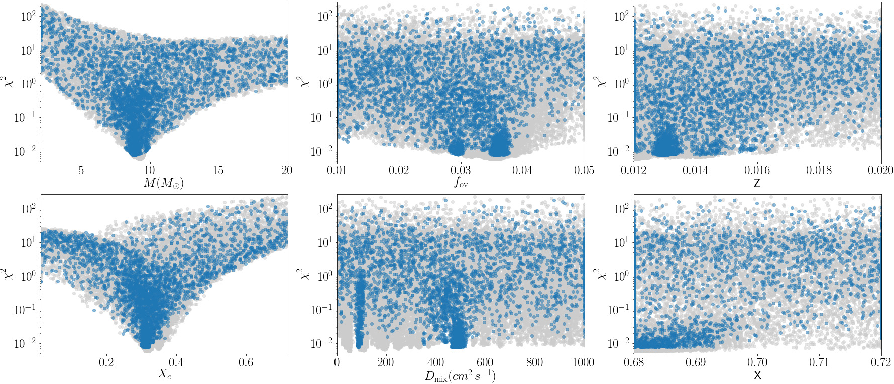
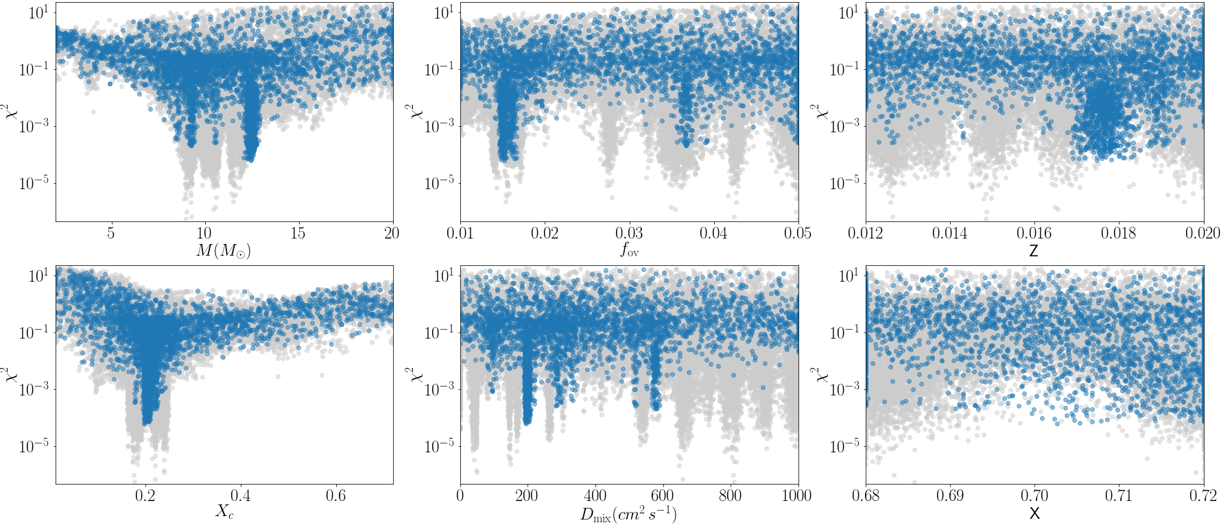
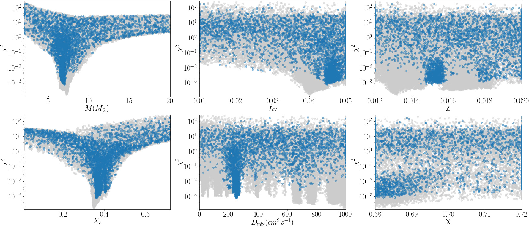
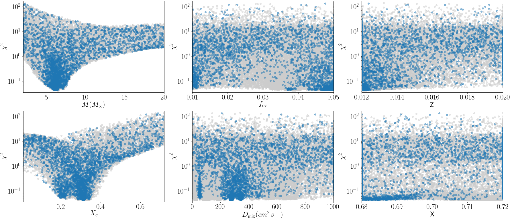
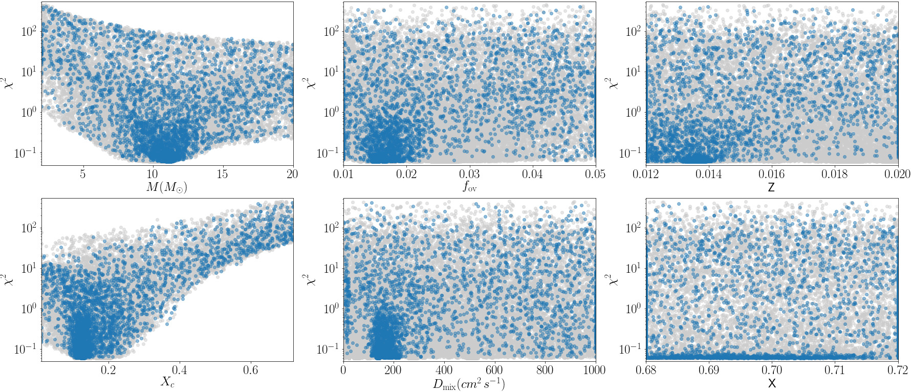
It is important to note that the particle filter could also be run on the actual simulation instead of the neural network in order to find the optimal combination of stellar parameters for a given list of frequencies. However, given the required amount of iterations to minimize the cost function this would be too time-consuming. Once the particle filter is used to find stellar parameters, the trained neural network is fixed and assumed to give correct output. This means the neural network is merely used as a fast replacement for the underlying physics simulator. The particle filter has seven hyperparameters. The choice of these determine how long the particle filter runs and how well it is able to find the global minimum. The choices of the hyperparameters are listed in Table 2. To illustrate the effect of different hyperparameters, two choices have been made and the results for both are in each case overplotted in the application figures below as gray and the blue points. The total amount of neural network inferences is . The goal of the particle filter is to find the global minimum in as few iterations as possible. The hyperparameter choices in Table 2 are found to be the most optimal combination to find the global minimum while keeping the total amount of neural network inference as low as possible. The blue points can be seen as a quick scan, where one finds the region of interest for the six stellar parameters. The gray points zoom in on the optimal combination more intensely. These values were found by incrementally increasing the hyperparameter values and evaluating the accuracy while keeping in mind that the number of evaluations should be as low as possible.
| Parameter | Gray | Blue |
|---|---|---|
| 5000 | 1000 | |
| 2000 | 100 | |
| 200 | 10 | |
| 10 | 10 | |
| 0.4 | 0.4 | |
| 0.1 | 0.1 | |
| 0.01 | 0.01 |
A visualization of the full pipeline is shown in Fig. 2. This method is able to find the minimum of a given set of measurements in about 30 seconds using an Nvidia GTX1080 GPU. Note that this excludes the training time of the actual neural network. However, the neural network only has to be trained once and then is applicable to all stars within the grid of the training dataset. The whole pipeline of finding the optimal set of stellar parameters using the particle filter and DNN is abbreviated below as the PF-DNN method.
6 Results
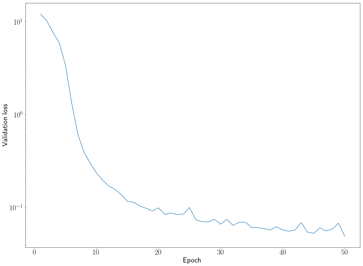
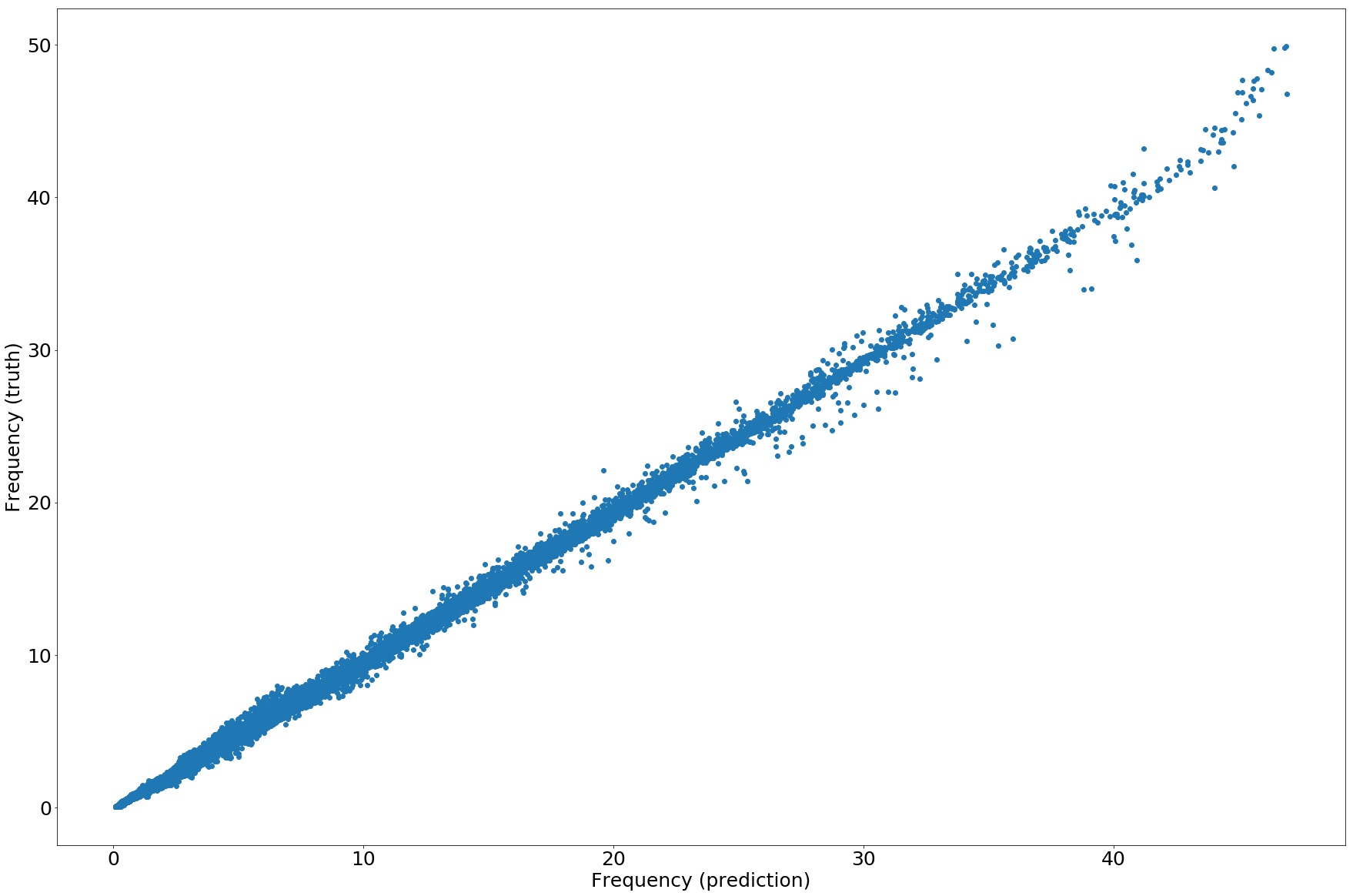
In Fig. 3 the loss on the validation set is plotted for 50 epochs. The mean-squared-error loss of the final result is 0.05. On an Nvidia GTX 1080 it takes around six hours to train the network. Figure 4 shows the predictive power of the neural network. As can be seen in the figure, the neural network almost always predicts the same frequency as is in the grid. Only for high frequencies the neural network underpredicts the frequency. This is probably due to an imbalance of the training data with respect to the frequency: in the plot are 100,000 random points from the validation set. As can be clearly seen, the distribution of frequencies is not flat. This could probably be improved by using for example pool based active learning, which will be explored in the next version of the pipeline.
As a proof-of-concept, the procedure defined in the previous sections is applied to seven selected slowly rotating stars of spectral type B for which forward asteroseismic modeling has been achieved in the past. We stress that our DNN is a preprocessing method, meant to provide a meaningful sub-space within a huge 6D grid of core hydrogen burning models with extensive coverage in mass, based on the input of a few (identified or not) coherent oscillation modes. If this works out, then we found a very fast way to define and start the computation of detailed and refined multi-D grids of stellar models for forward modeling, following the methodology of Paper I. Our approach and results have to be evaluated with this aim in mind.
We focus on five Cep stars with low-order pressure and gravity modes and two slowly pulsating B stars (SPBs) with high-order gravity modes. All seven pulsators are very slow rotators, such that we can limit to zonal modes (). While the past CoRoT and Kepler and current BRITE space missions delivered good asteroseismic data for several intermediate-mass SPBs (e.g., Pápics et al., 2017; Kallinger et al., 2017; Szewczuk & Daszyńska-Daszkiewicz, 2018), this was not the case for the more massive Cep stars. However, the TESS mission (Ricker et al., 2016, launched successfully on 18 April 2018) will deliver data of hundreds of such pulsators very soon.
An important remark is that the five Cep stars have been modeled asteroseismically with stellar evolution and pulsation codes that are completely independent from those that were used to construct the SpaceInn grid. They therefore constitute by far the most important test for our PF-DNN method, because the used model grid and the DNN methodology are both new and are built upon independent ingredients from the previous decade-old applications. The two SPBs were modeled with the MESA and GYRE codes, which also lie at the basis of the SpaceInn grid. For those, the test is therefore mainly at the level of the PF-DNN strategy, and not so much on the input physics of the model grid. Our major aim is to test if the PF-DNN method can derive appropriate ranges for the mass and evolutionary stage of the stars, keeping in mind that degeneracies occur between .
6.1 The Cep star HD 129929
Apart from the Sun, HD 129929 was the first star in the core hydrogen burning phase for which an asteroseismic estimate of the rotation rate in the stellar interior could be obtained (Aerts et al., 2003). This was achieved from 21 years of single-site multi-color photometric monitoring at mmag precision, which resulted in the detection of a radial mode, a dipole triplet, and two members of a quadrupole quintuplet (Aerts et al., 2004). A spectroscopic estimate of and added to the photometry led Dupret et al. (2004) to a near-core rotation frequency of 0.013 d-1 and a 4 times faster near-core than envelope rotation, in agreement with the spectroscopically measured . The authors also identified the need for non-zero yet low core overshooting. This phenomenon was modeled as convective penetration and required a step-overshoot value of (expressed in local pressure scale heights). Aside from the core overshooting, the star’s mass , metalicity (), and age (i.e., through ) were estimated (cf. Table 3). This asteroseismic forward modeling was done “manually” at a time when CPU power was much more limited than currently, by “meandering” in a sparse grid. Finding an appropriate asteroseismic model at that time required typically weeks/months to achieve, depending on the experience of the user.
| Parameter | PF-DNN Value (gray) | PF-DNN Value (blue) | Dupret et al. (2004) |
| (M⊙) | 9.23 | 8.81 | 9.35 |
| 0.0365 | 0.0356 | ||
| 0.012 | 0.0130 | ||
| 0.314 | 0.314 | 0.353 | |
| 48 | 475 | – | |
| 0.680 | 0.68 | 0.7 (fixed) |
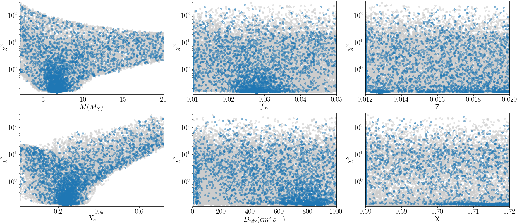
Here, we only use the three identified zonal () modes of HD 129929 (ignoring the spectroscopic information) as a first test case for our PF-DNN method. It concerns the observed frequencies 6.590940 d-1 with , 6.978305 d-1 with , and 6.461699 d-1 with (Aerts et al., 2003, 2004). The outcome is shown in the upper six panels of Fig. 5 and the parameters identified as “best” model by the trained network are presented in Table 3. First of all, one should not restrict to the bare minimum given by the PF-DNN method as listed in Table 3 but always consider the morphology of the whole PF-DNN outcome as in Fig. 5, as broad minima may occur. Moreover, we point out that the PF-DNN uses diffusive convective overshooting with the radiative temperature gradient in the overshoot zone rather than convective penetration with the adiabatic gradient. The relation between and is about a factor 10 to 12 (Moravveji et al., 2015; Claret & Torres, 2017) and must be taken into account when evaluating the PF-DNN capacity. Keeping this in mind, we deduce from Fig. 5 and Table 3 that the PF-DNN does a remarkably good job when considering the dense network (indicated as gray solution in Table 3), particularly keeping in mind that the metalicity cannot be well constrained from forward modeling of high-mass stars and that and are correlated in the case of B-type pulsators (e.g., Walczak et al., 2013; Moravveji et al., 2015; Pedersen et al., 2018). It can also be deduced from the six upper panels in Fig. 5 that the initial hydrogen content and the level of chemical mixing in the envelope are not well constrained. This is generally the case for the Cep stars treated here, and in particular for HD 129929, given that there are only three detected oscillation modes to estimate six parameters. The same limitation occurred from the manual forward modeling done 15 years ago.
For most applications, one does not know the radial order of the modes connected with the measured frequencies. Any first screening of models must then be based on the provision of the mode degrees , without providing the radial orders . We used the case of HD 129929 to test how the lack of values for affects the results. The outcome can be seen in the lower six panels of Fig. 5 and reveals that, without information on the radial order, one finds several sharp minima for the mass and evolutionary stage. The secondary minimum corresponds to a more massive and more evolved model for which the radial mode is the first overtone rather than the fundamental mode. This model has a somewhat lower convective core overshooting and is older. This exercise shows that, whenever the radial order of the modes is unknown quantitatively but only in terms of relative ranking among the detected frequencies, one can still get a good solution, but it is to be advised that the several options for the mass are considered for refined and detailed modeling, e.g. with the methods in Paper I.
6.2 The Cep star HD 157056
In terms of structure in the frequency spectrum, the Cep star HD 157056 is almost a copy of HD 129929 (Briquet et al., 2007), except that its detected rotational splitting is in agreement with rigid rotation with rotation frequency 0.107 d-1 throughout the star. This is eight times faster than the rotation of HD 129929, but still very slow compared to the periods of order hours of its low-order oscillation modes and far below its critical rotation rate. It is therefore still fine to ignore the effect of the Coriolis force on the oscillation frequencies, particularly for the zonal modes.
| Parameter | PF-DNN Value (gray) | PF-DNN Value (blue) | Briquet et al. (2007) |
| (M⊙) | 7.21 | 6.98 | 8.20.3 |
| 0.0402 | 0.0448 | ||
| 0.0132 | 0.0151 | ||
| 0.349 | 0.365 | ||
| 988 | 256 | – | |
| 0.680 | 0.686 |
The zonal oscillation-mode frequency values of HD 157056, i.e., 7.4677 d-1 for , 7.8742 d-1 for , and 7.204 d-1 for , are higher than the corresponding ones of HD 129929. Since it concerns zonal pressure modes, which are connected with standing acoustic waves, this implies that the star must be smaller and hence less massive than HD 129929. This was confirmed by the asteroseismic modeling results obtained by Briquet et al. (2007) listed in Table 4. A striking result found by these authors is the large value of for the core overshooting, where their models were based on convective penetration.
Briquet et al. (2007) also investigated models with atomic diffusion but in a description that ignores radiative levitation. It is well known that atomic diffusion in models of stars with a radiative envelope implies the helium and metals to sink too strongly, leading to incorrect surface abundances. One usually counter-balances this too strong settling by adding an amount of turbulent mixing in the superficial envelope layers. Briquet et al. (2007) showed that the inclusion of atomic diffusion along with such artificial turbulence, at a level that brings the predicted surface abundances in agreement with the observed values, does not change the asteroseismic parameter estimates appreciably.
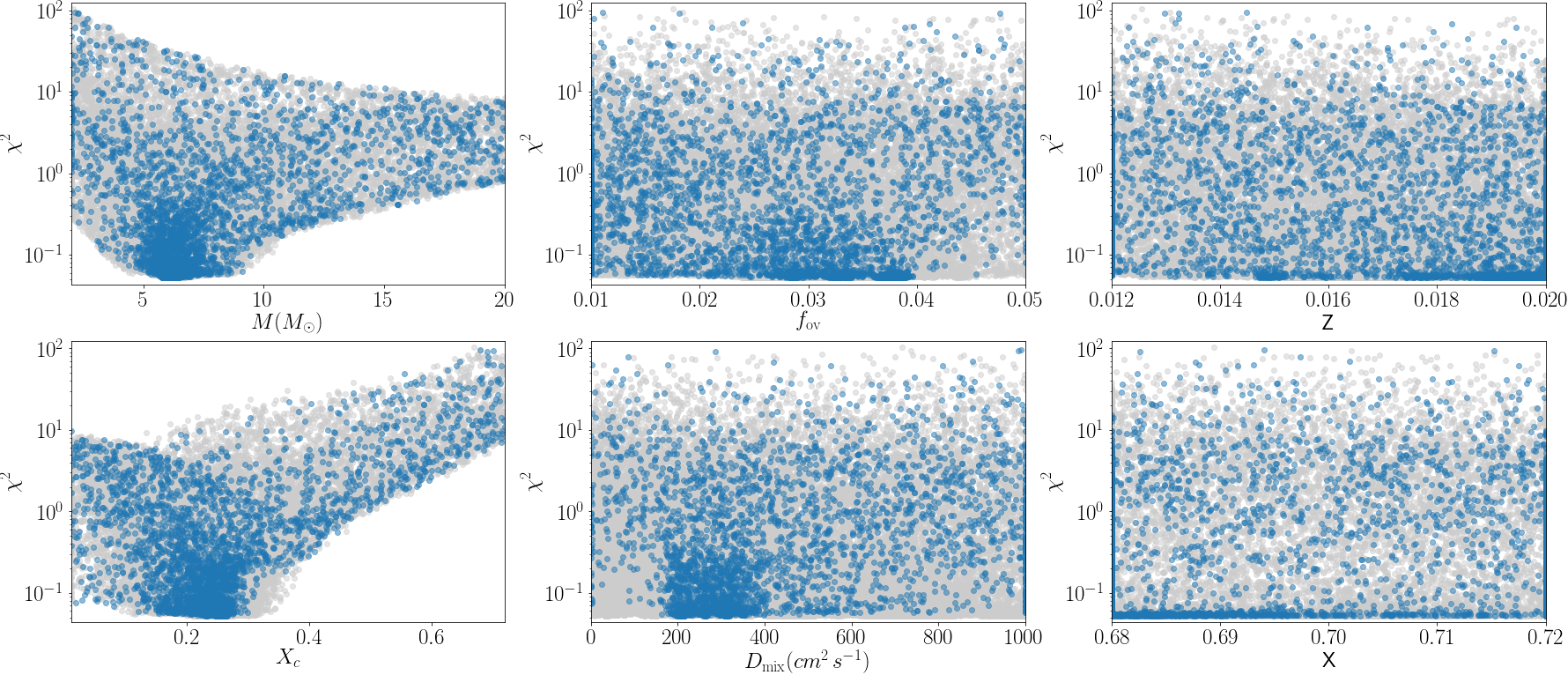
Our PF-DNN results of HD 157056 are shown in Fig. 6. In this case, it can be seen that a deep minimum and a secondary minimum for the mass occur for the blue dots, while one cleaner minimum occurs for the gray dots. The most important conclusion, however, is independent of which version of the DNN we adopt: as reported in Table 4, the DNN confirms the high level of core overshooting for this star. Further, the DNN results in a different combination and a 1 M⊙ lower mass compared to the forward modeling. It is well known that a mass-metalicity relation occurs when fitting low-order pressure modes in Cep stars (lower mass is accompanied by a higher metalicity: Fig. 2 in Ausseloos et al., 2004). Moreover, as already mentioned, the core overshooting and mass are also correlated. Taking this into account, the PF-DNN solution is appropriate. In particular, the PF-DNN manages to pinpoint the correct evolutionary stage of the star.
6.3 The Cep star HD 886
The Cep star HD 886 was long known to be a slowly rotating monoperiodic radial pulsator, but space photometry assembled with the MOST satellite revealed thirteen non-radial oscillation modes aside from the dominant radial mode. Among these thirteen frequencies are seven low-order modes and six gravity modes (Handler et al., 2009). While forward modeling has not been done for this star yet, Walczak et al. (2013) did make an extensive comparison of the observed oscillations and those predicted by theoretical models, with the main aim to test the mode excitation theory. They managed to identify five of the fourteen detected modes, assuming zonal modes: the three low-order modes with 6.58974 d-1 for , 6.01616 d-1 for , 9.1092 d-1 for , and the two high-order gravity modes with 0.8352 d-1 for , 0.63551 d-1 for . The parameters of their “Model 2” are listed in Table 5. For this star, the shift induced by rotation is less than 0.005 d-1 (Walczak et al., 2013) so that rotation can be ignored in the application.
| Parameter | PF-DNN Value (gray) | PF-DNN Value (blue) | Walczak et al. (2013) |
| (M⊙) | 6.43 | 6.13 | 7.9 |
| 0.0388 | 0.0499 | ||
| 0.012 | 0.012 | 0.0135 | |
| 0.312 | 0.312 | – | |
| 269 | 269 | – | |
| 0.68 | 0.68 | 0.71 (fixed) |
Our PF-DNN results of HD 886 are shown in Fig. 7 and the two minima of the network are listed in Table 5. Again, we find a lower mass compared with the interpretation of the frequencies in the literature (for the blue and gray dots). However, in this case Fig. 7 shows a broad mass range rather than a sharp minimum, so the disagreement with the mass reported in the literature is acceptable. Walczak et al. (2013) deduced a linear relationship between the core overshooting, the mass, and the metalicity for the mode frequencies of HD 866. Our PF-DNN results in Table 5 are in agreement with their results when taking into account that linear relationship, if we keep in mind the factor between and . Indeed, we find a lower mass and a lower metalicity than the values reported in Walczak et al. (2013), but we report a higher core overshoot. All in all, we also find good agreement between our PF-DNN results and the literature values for this third star.
6.4 The Cep star HD 29248
The Cep star HD 29248 is one of the most intensively studied pulsators of its class. From the observational side, it was the first target of major months-long multisite multitechnique campaigns involving tens of astronomers worldwide (see Jerzykiewicz et al., 2005, for a summary). That data led to the discovery of more modes than its radial mode and triplet, which were known prior to the multisite campaign. Among the new modes are two high-order gravity modes. Recently, these results were confirmed by BRITE space photometry, which led by itself to yet a few more mode detections, bringing the total to ten low-order modes and seven high-order gravity modes (Handler et al., 2017).
The star is also a relatively slow rotator, but the envelope rotation frequency does amount to d-1, i.e., slightly faster than HD 157056. Again, we assume that we can ignore the effect of the Coriolis force on the oscillation frequencies and we work with the identified zonal modes for application to the PF-DNN. In summary, identification of the zonal modes led to: 5.763264 d-1 for , 5.6373 d-1 for , 6.2434 d-1 for , and 7.9131 d-1 for (De Ridder et al., 2004). HD 29248 is the only Cep pulsator so far with the detection and identification of three dipole pressure modes of consecutive radial order.
The seven additional modes without mode identification have frequencies 0.6870 d-1, 0.4307 d-1, 0.3894 d-1, 0.3395 d-1, 0.3242 d-1, 0.2951 d-1, and 0.2648 d-1 (Handler et al., 2017). While their radial orders are not known, they must be decreasing in value (as these are gravity-mode frequencies whose ). We assumed those to have mode degree or 2 and have added them to the PF-DNN.
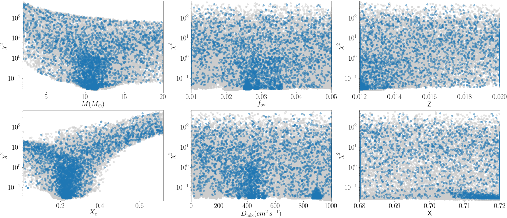
We applied the PF-DNN method twice: once for the case that the radial mode is the fundamental one with only identified modes and additionally by adding the unidentified gravity modes (see Fig. 8). From both applications, it can be seen from Fig. 8 that the addition of the unidentified high-order modes does not help the PF-DNN. This is not surprising as, in general, feeding the PF-DNN with unidentified modes does not provide constraints on the stellar parameters. The minima of the PF-DNN method for both cases (A: identified modes; B: non-identified mode frequencies added) are listed in Table 6, along with the results from seismic modeling in the literature based on the assumption of the fundamental radial mode (Ausseloos et al., 2004; Daszyńska-Daszkiewicz et al., 2017). First of all, it can be deduced that the parameters of the two minima (here only given for the densest PF-DNN) are very similar. Furthermore, this is again a case where the value of the strict minimum for the mass is not very meaningful, because a similarly low is found for a mass range between some 6 to 9 M⊙ is revealed in Fig. 8. This broad mass range corresponds with the one found by two independent studies in the literature (Ausseloos et al., 2004; Daszyńska-Daszkiewicz et al., 2017). Irrespective of the mass range, the PF-DNN method finds HD 29248 to be a rather evolved star, in agreement with the asteroseismic analyses by Ausseloos et al. (2004) and by Dziembowski & Pamyatnykh (2008). We also deduce that a large amount of extra diffusive envelope mixing occurs, an aspect that was so far not studied for this star.
| Parameter | Value A (gray) | Value B (gray) | Ausseloos et al. (2004) | Daszyńska-Daszkiewicz et al. (2017) |
|---|---|---|---|---|
| (M⊙) | 6.56 | 6.55 | 7.83 | |
| 0.0242 | 0.0255 | (fixed) | ||
| 0.0195 | 0.0159 | 0.0155 | ||
| 0.275 | 0.222 | – | – | |
| 770 | 1000 | – | – | |
| 0.716 | 0.699 | 0.70 (fixed) | 0.70 (fixed) |
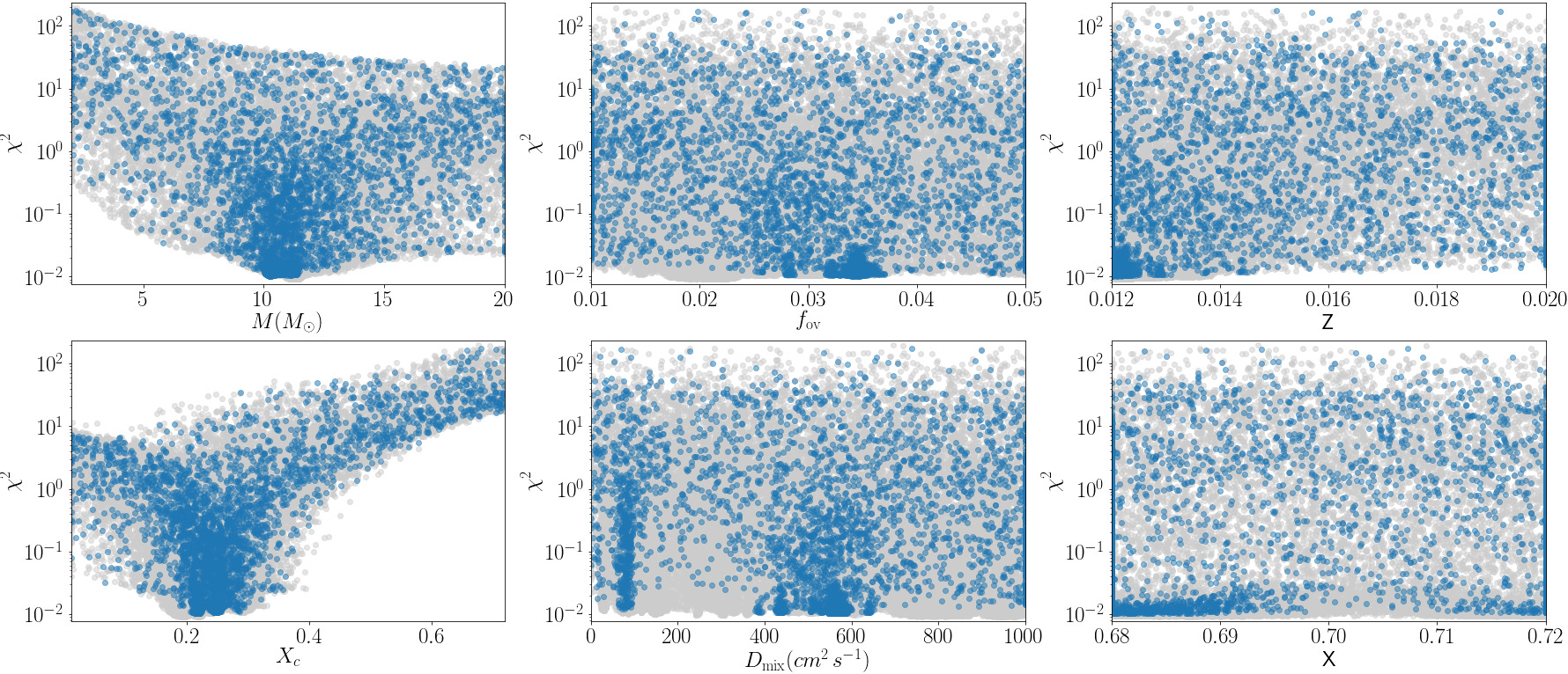
For this star, we did an additional test by feeding the PF-DNN with the case where the dominant radial mode would be the first overtone, increasing as well the of the modes with frequencies higher than the one of the radial mode. The outcome is shown in Fig. 9. As can be seen in that plot, and as expected astrophysically, the solutions found by the PF-DNN now belong to higher mass models. Also for this case, the addition of extra unidentified gravity-mode frequencies does not change the morphology and best solutions found by the PF-DNN. This exercise illustrates that the PF-DNN is well capable to distinguish among model parameters when the overtone of the radial mode is different.
6.5 The Cep star HD 214993
Along with HD 29248, the Cep pulsator HD 214993 has been the subject of extensive months-long multicolor photometric and high-resolution spectroscopic multisite campaigns. Its mode detection, mode identification and forward asteroseismic modeling based on those ground-based data sets are summarized in Handler et al. (2006); Dziembowski & Pamyatnykh (2008) and Desmet et al. (2009). In contrast to HD 29248, there is no high-precision uninterrupted space photometry available for HD 214993, so we used the oscillation modes identified from the multisite campaigns as input for the PF-DNN.
We made two applications for this star, based on the frequencies and mode identification in Table 8 of Desmet et al. (2009), i.e., assuming the radial mode to be the first overtone. These authors have deduced an average rotation frequency of the star equal to 0.1880.002 d-1, which is faster than the other Cep stars discussed so far. This implies that the validity of the SpaceInn grid of non-rotating models coupled to computations of the oscillation modes while ignoring the Coriolis force might become sub-optimal for HD 214993.
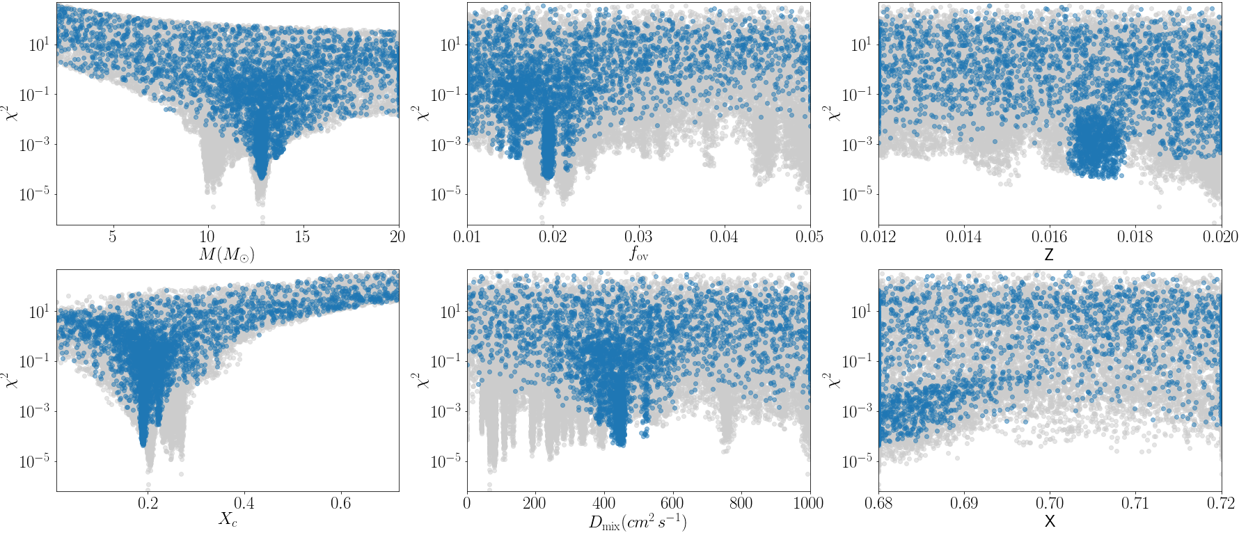
We first performed a PF-DNN scan using only the three zonal modes, as these are least affected by rotation. It concerns the modes of frequencies 5.334224 d-1 with , 5.066316 d-1 with , and 5.30912 d-1 with . The results of the PF-DNN for this case are shown in the upper six panels of Fig. 10. We recover good values for the mass, but find several minima for the core overshooting. Note that the “manual” forward modeling by Desmet et al. (2009) could not pinpoint a value for .
If we instead add the modes whose azimuthal order were identified as or unidentified, namely 5.490133 d-1 with , 4.241787 d-1 with , 6.702318 d-1 with , 7.407162 d-1 with , and 5.84511 d-1 with (Table 8, Desmet et al., 2009), then we find a lower mass, a lower metalicity and a higher core overshoot (Fig. 10). For this star, given it is a moderate rather than a slow rotator, we see that the addition of frequencies belonging to modes of , changes the morphology of solutions found by the PF-DNN. As a conclusion, the minima found by the PF-DNN for both cases give meaningful results when compared with the modeling results from Desmet et al. (2009), even for the relatively high rotation rate of 0.188 d-1 for this pulsator.
| Parameter | PF-DNN Value A (gray) | PF-DNN Value B (gray) | Desmet et al. (2009) |
| (M⊙) | 12.8 | 10.2 | |
| 0.0187 | 0.0262 | ||
| 0.0198 | 0.0132 | 0.015 (fixed) | |
| 0.200 | 0.174 | ||
| 66 | 279 | – | |
| 0.68 | 0.72 | 0.72 (fixed) |
6.6 The Kepler SPB star KIC 10526294
We now turn our attention to the more difficult case of high-order gravity modes in SPBs. These multiperiodic pulsators have been found since long from extensive ground-based photometry (Waelkens, 1991) and spectroscopy Aerts et al. (1999). However, given that the periodicities of their high-order gravity modes are half to several days, the beating patterns of the overall effect of the multiperiodic oscillations cover many years. It is therefore needed to have time-series data with a very long time base. Despite extensive ground-based campaigns covering many years, these data turned out to be of too low duty cycle and led to too few modes to perform forward asteroseismic modeling (cf., De Cat & Aerts, 2002). This capacity had to await the 4-year Kepler photometry, which revealed period-spacing patterns of the gravity modes. Such patterns allow to identify the mode degrees and estimate the radial orders .
Moravveji et al. (2015) performed the first forward seismic modeling of an SPB. Their target was the B8.3V star KIC 10526294, whose frequencies were derived from a 4-year long Kepler light curve by Pápics et al. (2014). The modeling was based on 19 detected dipole zonal modes with consecutive radial order (listed in Table 1 of Moravveji et al. (2015), and omitted here for brevity). These 19 modes reveal an average period spacing of 5,400 s. Their forward modeling led to identification of the radial orders ranging from -14 to -32. Based on the best equilibrium models, Triana et al. (2015) subsequently determined the star’s rotation profile throughout its interior from inversion methods applied to the rotationally split triplet frequencies. They found a counter-rotating profile that deviates only slightly from rigidity inside the star. KIC 10526294 was found to rotate exceptionally slowly for a B star, with an average rotation rate of only 0.0054 d-1. This star is therefore the ideal and so far only case to test the capacity of our PF-DNN method for stars that only exhibit high-order gravity modes and no pressure modes. Indeed, all other Kepler or BRITE SPBs with period spacing patterns have fast rotation (Pápics et al., 2017; Kallinger et al., 2017; Szewczuk & Daszyńska-Daszkiewicz, 2018) and cannot be treated with the SpaceInn grid.
| Parameter | PF-DNN Value (gray) | PF-DNN Value (blue) | Paper I |
|---|---|---|---|
| (M⊙ | 5.25 | 5.26 | 3.24 |
| 0.0348 | 0.0345 | 0.017 | |
| 0.0120 | 0.0120 | 0.017 | |
| 0.712 | 0.712 | 0.644 | |
| 798 | 996 | 178 | |
| 0.72 | 0.72 | 0.71 (fixed) |
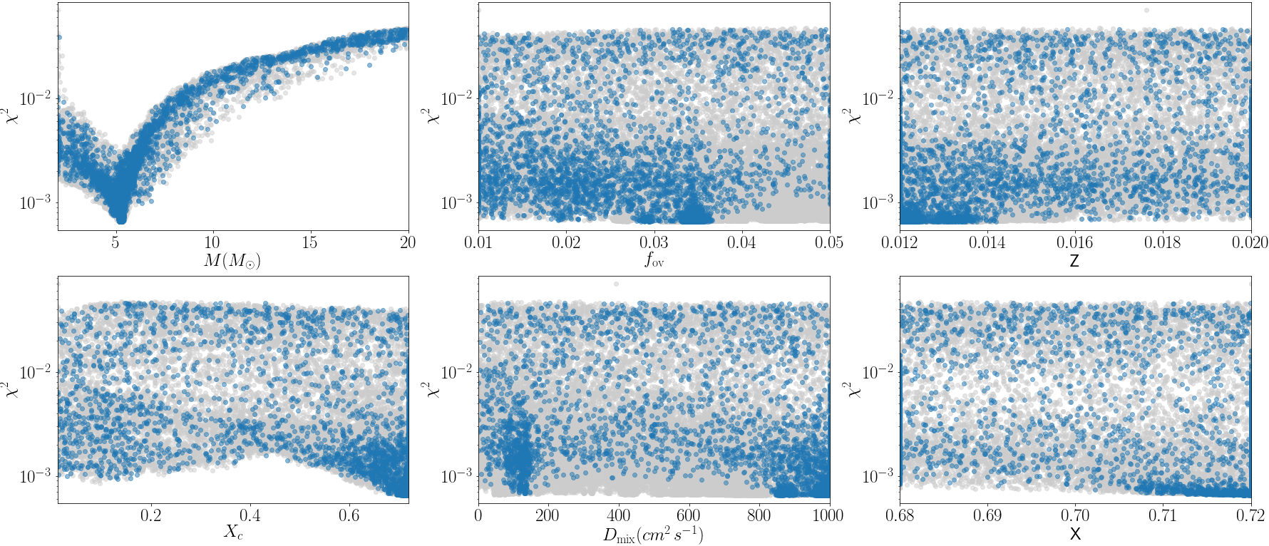
We fed the PF-DNN with the 19 zonal dipole mode frequencies and opted not to pinpoint the values to those found in Moravveji et al. (2015), but rather set the constraint that all the 19 modes must be of consecutive radial order. This is the best approach given that the mode spectrum for high-order gravity modes is very dense and labeling of is sometimes ambiguous for close frequency values. The outcome can be seen in Fig. 11 and the minima found by the two versions of the PF-DNN are listed in Table 8. We find a sharp minimum for the mass, but at a value about 2 M⊙ higher than the one obtained by a re-analysis of the forward modeling as presented in Paper I. However, the PF-DNN also finds a twice as high core overshoot parameter. Keeping in mind the degeneracy (cf. Fig. 5 in Moravveji et al., 2015), it is expected that a higher mass must be accompanied by a higher core overshoot. Moreover, the lower metalicity found by the PF-DNN must also be accompanied by a higher mass. Finally, the PF-DNN’s minima occur at the ZAMS (highest initial hydrogen () value), i.e., a border of the SpaceInn grid. Taking the degeneracies among the as in Fig. 5 of Moravveji et al. (2015), the PF-DNN solution is well understood but illustrates that its application to the high-order gravity modes of SPBs is less powerful than to the low-order pressure modes of Cep stars.
6.7 The CoRoT SPB HD 50230
The B3V star HD 50230 was the first main-sequence star for which a period spacing pattern of high-order gravity modes was discovered (Degroote et al., 2010). This discovery was based on 5 months of CoRoT space photometry and led to an average spacing of s from eight modes with consecutive radial order. From this average spacing, Degroote et al. (2010) derived a star of M⊙, which is relatively far evolved in its core-hydrogen burning stage (). The small and periodic deviation from the average period spacing made the authors conclude that convective penetration cannot be the only mixing phenomenon in the radiative envelope, as this would lead to a sharp -gradient in the near-core region and hence strong mode trapping. This is not observed for this star, hence the conclusion that diffusive envelope mixing must occur. A rough estimate of between 1,000 and 10,000 cm2 s-1 was suggested.
Regrettably, the CoRoT data is only five months in duration and this turns out to be a limitation for forward asteroseismic modeling (Paper I), unless one can get independent additional information on the degree of at least one mode (Buysschaert et al., 2018). This extra information is not available for HD 50230. Moreover, Degroote et al. (2012) discovered HD 50230 to be part of a spectroscopic binary with a wide orbit, which they did not manage to cover.
| Parameter | PF-DNN Value (gray) | PF-DNN Value (blue) | Degroote et al. (2010) |
| (M⊙) | 11.12 | 7.88 | |
| 0.0494 | 0.0494 | ||
| 0.02 | 0.0129 | 0.02 (fixed) | |
| 0.0453 | 0.173 | ||
| 32 | 1000 | – | |
| 0.716 | 0.68 | 0.71 (fixed) |
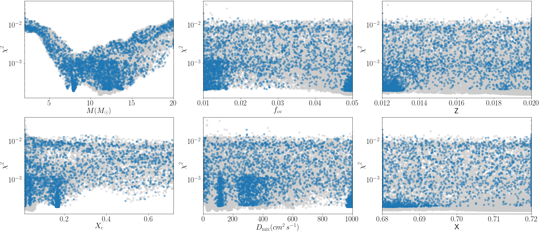
Here, we analysed HD 50230 with our PF-DNN and find an excellent solution from the less dense network (cf. Fig. 12). This is due to the fact that the denser one has a broad deeper minimum at a too high mass, corresponding with very old stellar models close to the end of the core-hydrogen burning. The deepest minimum of the less dense PF-DNN corresponds to very plausible parameters for this star and brings the first estimate of its large core overshooting and envelope mixing. Here, it is the average period spacing value that allows us to eliminate the too high mass solution. Without that information, any user would have to perform detailed forward modeling, keeping the two different minima for the mass in any more detailed follow-up study.
7 Conclusion and Future Prospects
We proposed a deep learning method as a starting point for the forward asteroseismic modeling of stars with coherent oscillation modes. A deep neural network was trained on an asteroseismological model grid containing more than 60 million theoretically predicted oscillation modes. Training the neural network has to be done once and then is applicable to all stars within the grid of the training set. This took around six hours on an Nvidia GTX 1080. By using a genetic algorithm over this trained neural network to find the maximum likelihood one can successfully find appropriate regions for the stellar parameters in a 6D space in less than a minute, relying only on detected and (partially) identified oscillation-mode frequencies. Our PF-DNN method was tested and applied to seven stars that were already modeled “manually” in the past. PF-DNN retrieved appropriate intervals for the parameters of those pulsators compared to the results available in the literature, keeping in mind known degeneracies between the stellar parameters.
Even though the DNN prediction is not perfect, it does reveal the regions in multi-D model space upon which to focus for more detailed screening. This method is therefore suitable as a first sampling strategy to constrain the possible complex parameter space. Indeed, the results of the network can be used as a seed point for more advanced applications of forward asteroseismic modeling following Paper I, for which the detailed and CPU-intensive computation of dedicated refined stellar model and pulsation grids as in, e.g., Moravveji et al. (2015) is necessary. Application of our method greatly helps the strategy and planning of such detailed grid computations after initial rough screening of the multi-D parameter space.
In a next step, we will generalize our PF-DNN method to rotating pulsating stars for which the Coriolis force cannot be neglected as we did here. This requires the addition of at least one dimension in the PF-DNN, namely the rotation frequency of the star. Accordingly, the shifts of the oscillation frequencies due to the Coriolis force must be computed for each of the modes in each of the models of the grid. While this is a serious complication, it also allows many more applications, given that most pulsators rotate at a frequency that cannot be neglected when fitting the measured non-zonal oscillation modes. Once our PF-DNN method is generalized to treat this case, it will be an appropriate starting tool to apply forward asteroseismic modeling with the statistical methodology of parameter estimation and model selection described in Paper I. This method by itself relies on a two-step approach: estimation of the rotation frequency of the star from detected multiplets of coherent modes (e.g., Kurtz et al., 2014; Pápics et al., 2014; Saio et al., 2015) and/or from period spacing patterns of high-order gravity modes (Van Reeth et al., 2016; Pápics et al., 2017; Ouazzani et al., 2017), followed by frequency fitting of all modes with identified degree and azimuthal order to within the measurement errors of the frequencies. Such a combined initial PF-DNN method followed by a statistical estimation and model selection approach offers an optimal way of forward asteroseismic modeling to be applied to many hundreds of pressure- and gravity-mode pulsators for which appropriate Kepler, TESS (Ricker et al., 2016), and PLATO (Rauer et al., 2014) data are or will become available in the near future.
In the next step, the PF-DNN method itself will be improved as well. A particular downside of the current setup is that the method does not contain uncertainty information. One can improve this by changing the DNN to a Bayesian DNN including aleatoric and epistemic uncertainties following the procedure of Kendall & Gal (2017). In that way, the maximum likelihood evaluation can be replaced with nested sampling (described in Skilling, 2004) to search the parameter space in a Bayesian context. This will provide not only a prediction of the model parameter ranges but contain uncertainty information as well. Such a procedure can then be followed by manual analyses zooming in on the selected region of interest, by allowing for various structural descriptions of core overshooting and mixing to derive their shape in the stellar interior, using the statistical methodology for stellar model performance comparison outlined as Problem Set 4 in Aerts et al. (2018).
References
- Abadi et al. (2015) Abadi, M., Agarwal, A., Barham, P., et al. 2015, TensorFlow: Large-Scale Machine Learning on Heterogeneous Systems, , , software available from tensorflow.org. https://www.tensorflow.org/
- Achterberg et al. (2015) Achterberg, A., Amoroso, S., Caron, S., et al. 2015, JCAP, 1508, 006
- Aerts et al. (2010) Aerts, C., Christensen-Dalsgaard, J., & Kurtz, D. W. 2010, Asteroseismology, Astronomy and Astrophysics Library, Springer Berlin Heidelberg
- Aerts et al. (2019) Aerts, C., Mathis, S., & Rogers, T. 2019, ARA&A, in press (arXiv1809.07779)
- Aerts et al. (2003) Aerts, C., Thoul, A., Daszyńska, J., et al. 2003, Science, 300, 1926
- Aerts et al. (1999) Aerts, C., De Cat, P., Peeters, E., et al. 1999, A&A, 343, 872
- Aerts et al. (2004) Aerts, C., Waelkens, C., Daszyńska-Daszkiewicz, J., et al. 2004, A&A, 415, 241
- Aerts et al. (2018) Aerts, C., Molenberghs, G., Michielsen, M., et al. 2018, ApJS, 237, 15
- Appourchaux (2014) Appourchaux, T. 2014, A crash course on data analysis in asteroseismology, ed. P. L. Pallé & C. Esteban, 123
- Appourchaux et al. (2012) Appourchaux, T., Chaplin, W. J., García, R. A., et al. 2012, A&A, 543, A54
- Asplund et al. (2009) Asplund, M., Grevesse, N., Sauval, A. J., & Scott, P. 2009, ARA&A, 47, 481
- Ausseloos et al. (2004) Ausseloos, M., Scuflaire, R., Thoul, A., & Aerts, C. 2004, MNRAS, 355, 352
- Auvergne et al. (2009) Auvergne, M., Bodin, P., Boisnard, L., et al. 2009, A&A, 506, 411
- Bellinger et al. (2016) Bellinger, E. P., Angelou, G. C., Hekker, S., et al. 2016, ApJ, 830, 31
- Bouabid et al. (2013) Bouabid, M.-P., Dupret, M.-A., Salmon, S., et al. 2013, MNRAS, 429, 2500
- Bowman (2017) Bowman, D. M. 2017, Amplitude Modulation of Pulsation Modes in Delta Scuti Stars, Jeremiah Horrocks Institute, University of Central Lancashire, Preston, UK. PhD Thesis published in Springer Theses series, doi:10.1007/978-3-319-66649-5
- Brassard et al. (2001) Brassard, P., Fontaine, G., Billères, M., et al. 2001, ApJ, 563, 1013
- Briquet et al. (2007) Briquet, M., Morel, T., Thoul, A., et al. 2007, MNRAS, 381, 1482
- Buysschaert et al. (2018) Buysschaert, B., Aerts, C., Bowman, D. M., et al. 2018, A&A, in press, arXiv:1805.00802
- Caron et al. (2018) Caron, S., Gómez-Vargas, G. A., Hendriks, L., & Ruiz de Austri, R. 2018, J. Cosmology Astropart. Phys, 5, 058
- Chauvin & Rumelhart (1995) Chauvin, Y., & Rumelhart, D. E., eds. 1995, Backpropagation: Theory, Architectures, and Applications (Hillsdale, NJ, USA: L. Erlbaum Associates Inc.)
- Claret & Torres (2017) Claret, A., & Torres, G. 2017, ApJ, 849, 18
- Corsaro & De Ridder (2014) Corsaro, E., & De Ridder, J. 2014, A&A, 571, A71
- Damien et al. (2016) Damien, A., et al. 2016, TFLearn, https://github.com/tflearn/tflearn, GitHub
- Daszyńska-Daszkiewicz et al. (2017) Daszyńska-Daszkiewicz, J., Pamyatnykh, A. A., Walczak, P., et al. 2017, MNRAS, 466, 2284
- Davies et al. (2016) Davies, G. R., Silva Aguirre, V., Bedding, T. R., et al. 2016, MNRAS, 456, 2183
- De Cat & Aerts (2002) De Cat, P., & Aerts, C. 2002, A&A, 393, 965
- De Ridder et al. (2004) De Ridder, J., Telting, J. H., Balona, L. A., et al. 2004, MNRAS, 351, 324
- Degroote et al. (2010) Degroote, P., Aerts, C., Baglin, A., et al. 2010, Nature, 464, 259
- Degroote et al. (2012) Degroote, P., Aerts, C., Michel, E., et al. 2012, A&A, 542, A88
- Deheuvels et al. (2016) Deheuvels, S., Brandão, I., Silva Aguirre, V., et al. 2016, A&A, 589, A93
- Desmet et al. (2009) Desmet, M., Briquet, M., Thoul, A., et al. 2009, MNRAS, 396, 1460
- Dupret et al. (2004) Dupret, M.-A., Thoul, A., Scuflaire, R., et al. 2004, A&A, 415, 251
- Dziembowski & Pamyatnykh (2008) Dziembowski, W. A., & Pamyatnykh, A. A. 2008, MNRAS, 385, 2061
- Gruberbauer et al. (2013) Gruberbauer, M., Guenther, D. B., MacLeod, K., & Kallinger, T. 2013, MNRAS, 435, 242
- Handler et al. (2006) Handler, G., Jerzykiewicz, M., Rodríguez, E., et al. 2006, MNRAS, 365, 327
- Handler et al. (2009) Handler, G., Matthews, J. M., Eaton, J. A., et al. 2009, ApJ, 698, L56
- Handler et al. (2017) Handler, G., Rybicka, M., Popowicz, A., et al. 2017, MNRAS, 464, 2249
- Herwig (2000) Herwig, F. 2000, A&A, 360, 952
- Iglesias & Rogers (1996) Iglesias, C. A., & Rogers, F. J. 1996, ApJ, 464, 943
- Jerzykiewicz et al. (2005) Jerzykiewicz, M., Handler, G., Shobbrook, R. R., et al. 2005, MNRAS, 360, 619
- Johnston et al. (2018) Johnston, C., Tkachenko, A., Aerts, C., et al. 2018, MNRAS, in press (arXiv1810.00780), arXiv:1810.00780
- Kallinger et al. (2017) Kallinger, T., Weiss, W. W., Beck, P. G., et al. 2017, A&A, 603, A13
- Kendall & Gal (2017) Kendall, A., & Gal, Y. 2017, CoRR, abs/1703.04977, arXiv:1703.04977. http://arxiv.org/abs/1703.04977
- Kingma & Ba (2014) Kingma, D. P., & Ba, J. 2014, CoRR, abs/1412.6980, arXiv:1412.6980. http://arxiv.org/abs/1412.6980
- Koch et al. (2010) Koch, D. G., Borucki, W. J., Basri, G., et al. 2010, ApJ, 713, L79
- Kurtz et al. (2014) Kurtz, D. W., Saio, H., Takata, M., et al. 2014, MNRAS, 444, 102
- Martins et al. (2012a) Martins, F., Escolano, C., Wade, G. A., et al. 2012a, A&A, 538, A29
- Martins et al. (2012b) Martins, F., Mahy, L., Hillier, D. J., & Rauw, G. 2012b, A&A, 538, A39
- Miglio & Montalbán (2005) Miglio, A., & Montalbán, J. 2005, A&A, 441, 615
- Miglio et al. (2008) Miglio, A., Montalbán, J., Noels, A., & Eggenberger, P. 2008, MNRAS, 386, 1487
- Moravveji et al. (2015) Moravveji, E., Aerts, C., Pápics, P. I., Triana, S. A., & Vandoren, B. 2015, A&A, 580, A27
- Moravveji et al. (2016) Moravveji, E., Townsend, R. H. D., Aerts, C., & Mathis, S. 2016, ApJ, 823, 130
- Morel et al. (2006) Morel, T., Butler, K., Aerts, C., Neiner, C., & Briquet, M. 2006, A&A, 457, 651
- Morel et al. (2008) Morel, T., Hubrig, S., & Briquet, M. 2008, A&A, 481, 453
- Murphy et al. (2016) Murphy, S. J., Fossati, L., Bedding, T. R., et al. 2016, MNRAS, 459, 1201
- Nair & Hinton (2010) Nair, V., & Hinton, G. E. 2010, in Proceedings of the 27th International Conference on Machine Learning (ICML-10), ed. J. Fürnkranz & T. Joachims (Omnipress), 807–814. http://www.icml2010.org/papers/432.pdf
- Ng (2004) Ng, A. Y. 2004, in Proceedings of the Twenty-first International Conference on Machine Learning, ICML ’04 (New York, NY, USA: ACM), 78–. http://doi.acm.org/10.1145/1015330.1015435
- Ouazzani et al. (2017) Ouazzani, R.-M., Salmon, S. J. A. J., Antoci, V., et al. 2017, MNRAS, 465, 2294
- Pápics et al. (2014) Pápics, P. I., Moravveji, E., Aerts, C., et al. 2014, A&A, 570, A8
- Pápics et al. (2012) Pápics, P. I., Briquet, M., Baglin, A., et al. 2012, A&A, 542, A55
- Pápics et al. (2017) Pápics, P. I., Tkachenko, A., Van Reeth, T., et al. 2017, A&A, 598, A74
- Paxton et al. (2011) Paxton, B., Bildsten, L., Dotter, A., et al. 2011, ApJS, 192, 3
- Paxton et al. (2013) Paxton, B., Cantiello, M., Arras, P., et al. 2013, ApJS, 208, 4
- Paxton et al. (2015) Paxton, B., Marchant, P., Schwab, J., et al. 2015, ApJS, 220, 15
- Paxton et al. (2018) Paxton, B., Schwab, J., Bauer, E. B., et al. 2018, ApJS, 234, 34
- Pedersen et al. (2018) Pedersen, M. G., Aerts, C., Pápics, P. I., & Rogers, T. M. 2018, A&A, in press, arXiv:1802.02051
- Quirion et al. (2010) Quirion, P.-O., Christensen-Dalsgaard, J., & Arentoft, T. 2010, ApJ, 725, 2176
- Rauer et al. (2014) Rauer, H., Catala, C., Aerts, C., et al. 2014, Experimental Astronomy, 38, 249
- Ricker et al. (2016) Ricker, G. R., Vanderspek, R., Winn, J., et al. 2016, in Proc. SPIE, Vol. 9904, Space Telescopes and Instrumentation 2016: Optical, Infrared, and Millimeter Wave, 99042B
- Saio et al. (2015) Saio, H., Kurtz, D. W., Takata, M., et al. 2015, MNRAS, 447, 3264
- Salaris & Cassisi (2017) Salaris, M., & Cassisi, S. 2017, Royal Society Open Science, 4, 170192
- Schmid & Aerts (2016) Schmid, V. S., & Aerts, C. 2016, A&A, 592, A116
- Silva Aguirre et al. (2017) Silva Aguirre, V., Lund, M. N., Antia, H. M., et al. 2017, ApJ, 835, 173
- Skilling (2004) Skilling, J. 2004, AIP Conference Proceedings, 735, 395. https://aip.scitation.org/doi/abs/10.1063/1.1835238
- Sowicka et al. (2017) Sowicka, P., Handler, G., Dȩbski, B., et al. 2017, MNRAS, 467, 4663
- Szewczuk & Daszyńska-Daszkiewicz (2018) Szewczuk, W., & Daszyńska-Daszkiewicz, J. 2018, MNRAS, in press, arXiv:1805.07100
- Townsend et al. (2018) Townsend, R. H. D., Goldstein, J., & Zweibel, E. G. 2018, MNRAS, 475, 879
- Townsend & Teitler (2013) Townsend, R. H. D., & Teitler, S. A. 2013, MNRAS, 435, 3406
- Triana et al. (2015) Triana, S. A., Moravveji, E., Pápics, P. I., et al. 2015, ApJ, 810, 16
- Van Reeth et al. (2016) Van Reeth, T., Tkachenko, A., & Aerts, C. 2016, A&A, 593, A120
- Van Reeth et al. (2015) Van Reeth, T., Tkachenko, A., Aerts, C., et al. 2015, ApJS, 218, 27
- Waelkens (1991) Waelkens, C. 1991, A&A, 246, 453
- Walczak et al. (2013) Walczak, P., Daszyńska-Daszkiewicz, J., Pamyatnykh, A. A., & Zdravkov, T. 2013, MNRAS, 432, 822