The Borg Cube Simulation: Cosmological Hydrodynamics with CRK-SPH

Abstract

A challenging requirement posed by next-generation observations is a firm theoretical grasp of the impact of baryons on structure formation. Cosmological hydrodynamic simulations modeling gas physics are vital in this regard. A high degree of modeling flexibility exists in this space making it important to explore a range of methods in order to gauge the accuracy of simulation predictions. We present results from the first cosmological simulation using Conservative Reproducing Kernel Smoothed Particle Hydrodynamics (CRK-SPH). We employ two simulations: one evolved purely under gravity and the other with non-radiative hydrodynamics. Each contains $2\times 2304^{3}$ cold dark matter plus baryon particles in an $800\text{\,}\Mpch$ box. We compare statistics to previous non-radiative simulations including power spectra, mass functions, baryon fractions, and concentration. We find self-similar radial profiles of gas temperature, entropy, and pressure and show that a simple analytic model recovers these results to better than $40\%$ over two orders of magnitude in mass. We quantify the level of non-thermal pressure support in halos and demonstrate that hydrostatic mass estimates are biased low by $24\%$ ($10\%$) for halos of mass $10^{15}~{}(10^{13})\text{\,}\massh$. We compute angular power spectra for the thermal and kinematic Sunyaev-Zel’dovich effects and find good agreement with the low-$\ell$ Planck measurements. Finally, artificial scattering between particles of unequal mass is shown to have a large impact on the gravity-only run and we highlight the importance of better understanding this issue in hydrodynamic applications. This is the first in a simulation campaign using CRK-SPH with future work including subresolution gas treatments.

h^-1M_⊙ h^-1Mpc h^-1kpc km s^-1 h Mpc^-1 GHz arcmin^2 deg^2

1. Introduction

It has been twenty years since the discovery of the accelerated expansion of the universe driven by dark energy (Riess et al., 1998; Perlmutter et al., 1999). Today, the nature of dark energy remains unknown on a fundamental level despite the fact that it presently dominates the Universe’s energy budget at a level of $\approx 70\%$ (e.g., Planck Collaboration et al., 2014). This puzzle has motivated a concerted effort to investigate the nature of dark energy through its influence on the expansion and structure growth histories of the universe (see e.g., Weinberg et al., 2013, for a recent review) enabled by current and upcoming sky surveys that provide large-scale structure statistics at unprecedented levels of detail and statistical precision. These campaigns include BOSS (Baryon Oscillation Spectroscopic Survey; Dawson et al., 2013), DES (Dark Energy Survey; The Dark Energy Survey Collaboration, 2005), DESI (Dark Energy Spectroscopic Instrument; Levi et al., 2013), LSST (Large Synoptic Survey Telescope; LSST Science Collaboration et al., 2009), Euclid (Laureijs et al., 2011), and WFIRST (Wide-Field InfraRed Survey Telescope; Spergel et al., 2013). Given the very low level of statistical uncertainty in the observations, theoretical and modeling systematics are a significant source of concern – as are measurement systematics – when considering the ultimate limits on the scientific information that can be gleaned from the surveys. It is therefore necessary that theory, modeling, and simulations be developed to a new level of detail and robustness in order to meet the varied challenges posed by next-generation observations.

The corresponding computational challenge is formidable due to the extreme range of spatio-temporal scales over which accurate predictions are needed. Generally speaking, we need to model volumes comparable to survey depths with sufficient resolution to capture the scales relevant for galaxy formation. The essential tools for this task are cosmological simulations that probe the deeply nonlinear regime of structure formation. The simplest examples are $N$-body simulations where the dynamics are dictated solely by gravitational forces. These simulations have become ubiquitous in the field and have proven useful in a wide variety of applications. The common convention assumes a potential dominated by cold dark matter (CDM) though other models inducing large changes on small scales such as warm dark matter or modified gravity scenarios are also studied. In any case, one certainly important omission in gravity-only (GO) simulations are contributions from baryons. In contrast to dark matter, baryons can dissipate energy, allowing them to cool and condense on small scales. The ensuing star formation and feedback from supernova and active galactic nuclei (AGN) have the potential to alter the matter distribution on small to moderately large scales. Separating the effects of complex astrophysical mechanisms from the fundamental physics associated with dark energy (and potentially dark matter physics at small scales) is essential for the proper interpretation of observations.

To this end, numerous cosmology codes are equipped with hydrodynamic solvers to model baryonic physics. Typically, this is done using either particle-based Lagrangian methods with smoothed particle hydrodynamics (SPH) (e.g., GADGET; Springel 2005, ASURA; Saitoh et al. 2008, GASOLINE; Wadsley et al. 2017), or mesh-based Eulerian methods on a stationary grid with possible adaptive mesh refinement (AMR) (e.g., ART; Kravtsov et al. 1997, RAMSES; Teyssier 2002, Nyx; Almgren et al. 2013, ENZO; Bryan et al. 2014). Hybrid schemes incorporating features of both SPH and AMR also exist (AREPO; Springel 2010, GIZMO; Hopkins 2015).

The most basic use case is that of non-radiative (NR) or “adiabatic” hydrodynamics in which the thermal state of baryons changes only in response to gravitational shock heating and adiabatic cooling with the expansion of the universe. While the pure NR case is a simplified description of the real universe that omits a number of important physics, it is still accurate on large to quasi-small length scales ($k\lesssim$1\text{\,}\invMpch$$). For instance, Burns et al. (2010) showed that NR simulations are sufficient to match the thermodynamic properties of gas on the outskirts of observed clusters. Moreover, NR physics is the natural first step of a hydrodynamics solver since this represents the most parameter-free reference point for comparison with other codes. Unfortunately, even in this most simple case, the Santa Barbara code comparison project (Frenk et al., 1999) showed that systematic differences arise between Eulerian and Lagrangian methods when simulating a massive galaxy cluster. The more recent nIFTy code comparison project (Sembolini et al., 2016) showed that much of this discrepancy has been resolved with modern SPH treatments matching more closely with mesh codes, though small differences still exist. Code comparisons like these are important in quantifying the level of confidence in simulation results. This becomes increasingly true as more complicated physics such as cooling and feedback are added, since these treatments vary substantially amongst codes.

It is therefore important to proceed in a controlled manner when designing a new cosmological hydrodynamics code. This paper is the first in a series to expand the gravitational framework of the Hardware/Hybrid Accelerated Cosmology Code (HACC; Habib et al., 2016) with a hydro solver equipped with a full suite of subresolution gas physics models capable of scaling to the problem size demanded by upcoming observations. Here we begin with an exclusive focus on the NR case, which serves as an important first step in the systematic process of modeling all of the baryonic physics relevant on cosmological scales. We perform both NR and GO simulations in large volumes with high mass resolution and compare to previous NR simulations to evaluate where we stand in relation to other methods. Furthermore, the large simulation volume used here allows us to significantly expand the statistical analysis of group and cluster-scale halos compared to previous NR runs that used smaller boxes. Similarly, the large box resolves additional power from low-$k$ density and velocity modes, enabling the construction of more accurate synthetic sky maps such as the thermal and kinematic components of the Sunyaev-Zel’dovich effect.

We employ a hydro solver based on the Conservative Reproducing Kernel Smoothed Particle Hydrodynamics (CRK-SPH; Frontiere et al., 2017) algorithm. CRK-SPH is a modern SPH treatment that overcomes two of the main shortcomings of traditional SPH (tSPH); namely, zeroth-order inaccuracy and an overly aggressive artificial viscosity. Frontiere et al. (2017) demonstrate this method to work robustly on a wide range of hydrodynamic tests including those with strong shocks and dynamical fluid instabilities. In addition, Raskin & Owen (2016) recently showed it to outperform standard SPH treatments in the astrophysically relevant case of a generalized rotating disk. Here we present results from the first use of CRK-SPH in a large-scale cosmological setting and show that it agrees well with other modern methods.

The incorporation of CRK-SPH into HACC has been designed from the outset for high performance and full scalability on next-generation supercomputers and is capable of running on all current high performance computing architectures. We refer to the new gravity plus hydro framework as CRK-HACC and provide technical details of its implementation as well as results from test cases such as the Santa Barbara run in Frontiere et al. (in prep.).

This paper is organized as follows. In Section 2, we provide details of the simulation setup and an overview of our numerical methods. Section 3 presents summary statistics from the main run with an emphasis on comparisons between the NR and GO cases. These include power spectra, halo mass functions, baryon fractions, and halo concentrations. Section 4 examines the gaseous components of halos and shows that a simple analytic model is able to match the simulated density, temperature, entropy, and pressure profiles with reasonably high accuracy. Section 5 measures the hydrostatic mass bias and fraction of non-thermal pressure support for group and cluster-scale halos. Section 6 provides an analysis of the thermal and kinematic components of the Sunyaev-Zel’dovich effect. We finish with a summary and conclusions of our work in Section 7.

2. Numerical Method

We perform two simulations utilizing the same initial conditions in order to compare the GO and NR cases of structure formation. Both simulations evolve $2304^{3}$ each of CDM and baryon particles in a box of side length $800\text{\,}\Mpch$ from redshift $z=200$ to 0. Each species is initialized on a uniform mesh and displaced using the Zel’dovich approximation (Zel’dovich, 1970) with a random realization drawn from the combined CDM plus baryon transfer function generated using CAMB (Lewis et al., 2000). The initial CDM and baryon meshes are maximally offset by staggering them by half the mean interparticle separation in each dimension. This is done to minimize artificial particle coupling in the initial conditions (Yoshida et al., 2003). Both meshes draw from the same white noise field and we account for the phase shift in the staggered grid when assigning displacements and velocities (Valkenburg & Villaescusa-Navarro, 2017). Finally, we set the initial thermal energy of baryons in the NR run to a uniform temperature of $847\text{\,}\mathrm{K}$ so as to match the adiabatic relation of gas that follows the cosmic microwave background (CMB) temperature until decoupling and adiabatically cooling at $z=129$.

The GO simulation is performed using HACC as a standard $N$-body run with dynamics based solely on gravity. The NR simulation is run with CRK-HACC and subjects baryons to both gravitational and hydrodynamic forces. We refer to the pair of runs as the Borg Cube simulations. Henceforth, quantities associated with the GO run are appended with a “go” subscript while quantities without subscripts refer to the NR case. Throughout our work, we employ the best-fit WMAP-7 cosmology (Komatsu et al., 2011) with ($\Omega_{c}$, $\Omega_{b}$, $\Omega_{\Lambda}$, $\Omega_{\nu}$, $w$, $n_{s}$, $\sigma_{8}$, $h$) = (0.22, 0.0448, 0.7352, 0, -1, 0.963, 0.8, 0.71), which was previously used in the Q Continuum (Heitmann et al., 2015), Outer Rim (Habib et al., 2016), and Mira Universe (Heitmann et al., 2016) simulations run with HACC. Particle masses in each simulation are $m_{c}=$2.56\times 10^{9}\text{\,}\massh$$ and $m_{b}=$5.21\times 10^{8}\text{\,}\massh$$ for CDM and baryons, respectively. This allows for individual group and cluster-scale halos (i.e., masses $\gtrsim$10^{13}\text{\,}\massh$$) to be resolved with at least thousands of particles. Moreover, with 138,000 such halos at $z=0$, we are able to stack halo profiles in multiple mass bins to obtain much more statistically robust results compared to previous simulations run with smaller simulation volumes. The gas in the NR run is modeled using an adiabatic index $\gamma=5/3$ with all CRK-SPH parameters (Courant factor, viscosity coefficients, etc.) following directly from Frontiere et al. (2017).

The gravitational force resolution is determined by the softening length. For multi-species runs, one must be careful to find a balance in force softening that mitigates artificial coupling between particles of unequal mass (Angulo et al., 2013) while maintaining adequate resolution. On the one hand, too small softening will cause low-mass particles to scatter off their high-mass counterparts. On the other hand, too large softening will inhibit structure growth on small scales due to the oversmoothing. For the Borg Cube runs, we use a Plummer softening length of $r_{\rm soft}=$14\text{\,}\kpch$$ (in comoving units), which is $1/25$ of the mean interparticle separation. This is held constant in time and between all particle pairs. One alternative approach involves using the SPH smoothing length to set a spatially adaptive softening length. The downside of this approach is that CDM-baryon gravitational interactions are heavily suppressed at early times when the particle distribution is relatively homogeneous so that the smoothing length is comparable to the mean interparticle separation (Angulo et al., 2013; Villaescusa-Navarro et al., 2017).

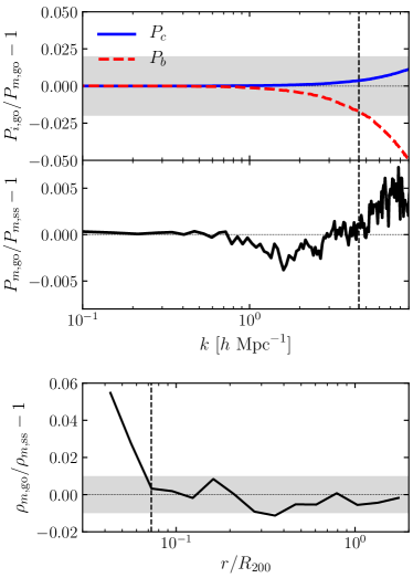
Figure 1.— Top panel shows the difference in power for the CDM (solid blue) and baryon (dashed red) components of the down-scaled GO run relative to the total matter at $z=0$. Deviations are within $\pm 2\%$ up to half the particle Nyquist frequency which is denoted by the vertical dashed black line. The peeling away of the the two components for $k\gtrsim$1\text{\,}\invMpch$$ is caused by artificial scattering between the two species. This run used a constant $r_{\rm soft}=$14\text{\,}\kpch$$; deviations become stronger and shifted to larger scales for finer softening. Middle panel compares the total matter from the down-scaled GO and SS runs at $z=0$. Although the individual components of the GO run experience percent-scale deviations, the total matter remains relatively unchanged compared to the SS case. Bottom panel compares stacked radial profiles of the total matter density for all halos with masses between $10^{13}-10^{13.5}\text{\,}\massh$ for the GO and SS runs at $z=0$. The profiles are truncated below $r_{\rm soft}$ and the vertical dashed line denotes the scale $30\text{\,}\kpch$ above which the profiles agree to roughly $1\%$.

Our choice of $r_{\rm soft}$ was made by finding the smallest value in the GO run such that differences in the CDM and baryon power relative to the total matter are within $2\%$ up to half the particle Nyquist frequency. This was achieved by experimenting on a down-scaled version of the Borg Cube with $2\times 288^{3}$ particles in a box of side length $100\text{\,}\Mpch$. The top panel of Figure 1 shows the relative difference in power for each component in the fiducial case where $r_{\rm soft}=$14\text{\,}\kpch$$. Ideally, we expect the two species to have identical power since they were initialized with the same transfer function and hydro forces are absent. Instead, scattering between heavy CDM and light baryons induces an enhancement (suppression) in power for the former (latter) on small scales. Using a smaller softening amplifies these deviations and shifts the onset of the problem to larger scales.

Interestingly, this artificial mass segregation operates in such a way that the total matter distribution is relatively unchanged. To show this, we ran a single-species (SS) simulation with $1\times 288^{3}$ particles representing the combined CDM plus baryon field (i.e., the setup of a traditional $N$-body simulation). The middle panel of Figure 1 compares the total matter power from the GO and SS runs; differences are sub-percent on all scales. Angulo et al. (2013) note a similar finding in their investigation of particle coupling in GO simulations. This invariance also emerges when examining radial profiles of the total matter content within halos. The bottom panel of Figure 1 shows the relative difference between GO and SS density profiles stacked over all halos in the mass range $10^{13}-10^{13.5}\text{\,}\massh$ (208 halos in GO; 206 in SS). These agree to about $1\%$ down to $r=$30\text{\,}\kpch$\approx 2r_{\rm soft}$. On smaller scales, the GO simulation displays systematically higher density at a level approaching $6\%$ at $r_{\rm soft}$.

We reiterate that this analysis was focused on suppressing the effects of mass segregation resulting from artificially strong interactions between unequal mass particles. In principle, other discreteness effects (e.g., strong interactions between particles of equal mass) that would also impact ordinary SS $N$-body simulations could also be present here. Such discreteness effects are an important topic (see, e.g., Melott, 2007; Power et al., 2016) and we leave to future work a more thorough investigation of their impact specifically in regard to hydrodynamic simulations.

Another important aspect to consider is the relationship between gravitational and hydrodynamic resolutions. As mentioned earlier, we use a constant softening length for all particle pairs, including both CDM and baryons. This means that there is a mismatch between the constant gravitational force resolution and the changing hydrodynamic resolution set by the adaptive SPH smoothing lengths, $h$. In this case, one must be careful to avoid the situation where $h$ drops below $r_{\rm soft}$ since this results in an unphysical numerical setup with hydrodynamics being evolved below the resolution limit of gravity. The alternate case where $h>r_{\rm soft}$ can also lead to unphysical fragmentation of gas clouds in the event that $h$ is close to the Jeans length (Bate & Burkert, 1997). Both of these scenarios are avoided here since the minimum smoothing length measured in the Borg Cube is $h_{\rm min}=$26\text{\,}\kpch$\approx 2r_{\rm soft}$ and the cosmological Jeans length is much smaller than the scales resolved here. Of course, it will be important to revisit this topic in future work with additional physics since cooling will significantly reduce $h_{\rm min}$ and other conditions – such as ensuring that the critical density for star formation is correctly resolved (e.g., Hopkins et al., 2018) – must be met.

Much of our analysis requires the identification of halos. This is achieved in a two-step fashion using the CosmoTools parallel analysis framework within HACC. First, we run a friends-of-friends (FOF) finder with a linking length of $b=0.168$. This is done only on the CDM particles to ensure that each particle in the FOF group has the same mass. We designate the halo center as the location of the most bound CDM particle in the FOF group. The next step is to create spherical overdensity (SO) halos by starting at the location of each FOF center and moving outwards in spherical shells until we reach the radius, $R_{200}$, at which the interior density is 200 times the critical density of the universe. These SO halos are constructed out of both CDM and baryon tracer particles. We show later that halo properties are converged for masses $M_{200}\geq$10^{13}\text{\,}\massh$$, corresponding to a combined mass of roughly $3200(m_{c}+m_{b})$. A thousand-particle threshold minimum for converged halo properties is also typical of single-species $N$-body simulations (e.g., Power et al., 2003; Child et al., 2018).

The central density of a halo is often described in terms of its concentration. This is defined as $c_{200}\equiv R_{\rm 200}/R_{s}$ where $R_{s}$ is the scale radius of the SO halo. A common convention is to find the concentration that matches the best-fit Navarro-Frenk-White (NFW; Navarro et al., 1997) density profile of the halo. While an NFW form is still mostly justified in the NR case, large deviations occur once sophisticated gas treatments such as radiative cooling and feedback are included (Rasia et al., 2013). In order to facilitate comparison with such cases, we opt for a concentration definition that is independent of the underlying density profile. Moreover, this allows us to compute concentrations for the baryon component of each SO halo separately, which will deviate strongly from an NFW form even in the NR case.

In what follows, we use the “peak finding” concentration method described in Child et al. (2018). The procedure is to find the radius, $R_{\rm peak}$, at which the differential mass profile, $dM/dr$, is a maximum and to define $c_{200}\equiv R_{200}/R_{\rm peak}$. This is achieved during halo-finding by first computing $dM/dr$ in 20 logarithmically-spaced spherical shells around each halo. A three-point Hann filter is used to smooth the differential mass profile and the bin with the maximum value is identified. If this bin is an endpoint, we set $R_{\rm peak}$ as the radius of the shell; otherwise, we fit a cubic spline to the bin and one adjacent neighbor in each direction to numerically solve for the peak.

Table 1Simulation Parameters for the Main Runs Referenced in this Work

Simulation	Reference	Code	$\Omega_{c}$	$\Omega_{b}$	$\sigma_{8}$	$n_{s}$	$h$	$L_{\rm box}$	$N_{c,b}$	$m_{c}$	$m_{b}$
								$\mathit{h}^{-1}$Mpc		$\mathit{h}^{-1}M_{\odot}$	$\mathit{h}^{-1}M_{\odot}$
Borg Cube	This Paper	CRK-HACC	0.22	0.0448	0.8	0.963	0.71	800	$2304^{3}$	$2.56\times 10^{9}$	$5.21\times 10^{8}$
J06	Jing et al. (2006)	GADGET	0.224	0.044	0.85	1.0	0.71	100	$512^{3}$	$4.64\times 10^{8}$	$9.11\times 10^{7}$
Illustris NR	Vogelsberger et al. (2014)	AREPO	0.227	0.0456	0.809	0.963	0.704	75	$910^{3}$	$3.53\times 10^{7}$	$7.10\times 10^{6}$
Illustris TNG	Springel et al. (2018)	AREPO	0.2603	0.0486	0.8159	0.9667	0.6774	205	$2500^{3}$	$3.99\times 10^{7}$	$7.45\times 10^{6}$
B10 NR	Battaglia et al. (2010)	GADGET	0.207	0.043	0.8	0.96	0.72	165	$256^{3}$	$1.54\times 10^{10}$	$3.20\times 10^{9}$
B10 Feedback	Battaglia et al. (2010)	GADGET	0.207	0.043	0.8	0.96	0.72	165	$256^{3}$	$1.54\times 10^{10}$	$3.20\times 10^{9}$

In the following sections, we compare results from the Borg Cube to other cosmological hydrodynamic simulations. Table LABEL:table:sims provides a useful summary of the main simulations referenced here. In each case, we list the code used, the cosmology assumed, the box width, particle count, and mass resolution for both CDM and baryons. The box size is in units of $\Mpch$ while particle masses are in units of $\massh$. The hydro solvers compared are the CRK-SPH scheme of CRK-HACC, the tSPH implementation in GADGET, and the moving mesh method of AREPO. All of the simulations are run in the NR regime except for Illustris TNG and B10 Feedback which both include additional prescriptions for radiative cooling and feedback from supernovae plus AGN. The simulations span three orders of magnitude in volume and mass resolution with the Borg Cube having the largest volume and a mass resolution suitable for group and cluster-scale halos.

3. Summary Statistics

3.1. Power Spectra

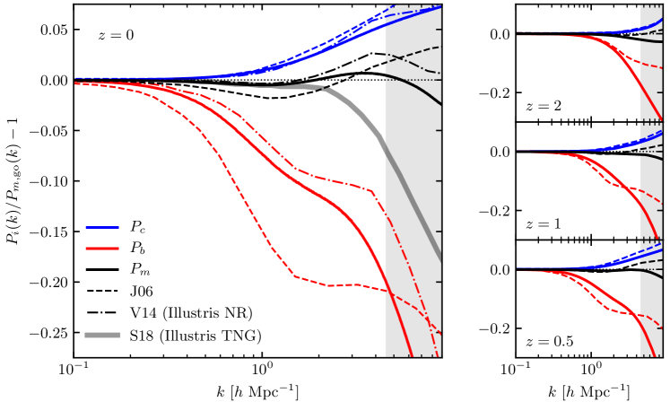
Figure 2.— Ratio in power spectra for the CDM (blue), baryon (red), and total matter (black) components of the NR simulation relative to the total matter result in the GO case. Solid lines are from the Borg Cube simulation while the dashed and dash-dotted lines show corresponding results from the NR simulations of Jing et al. (2006) and Vogelsberger et al. (2014), respectively. The thick shaded line in the $z=0$ panel traces the total matter result from the Illustris TNG cooling plus feedback simulation presented in Springel et al. (2018). Note that the ratio in power for each set of simulations is measured with respect to their own corresponding GO run. The vertical shaded band in each panel denotes scales above half the particle Nyquist frequency of the Borg Cube run.

We begin with an investigation of how NR processes affect the density power spectrum. In Figure 2, we plot the ratio in power for each component in the NR simulation relative to the total matter power in the GO run. For comparison, we show the results from the NR simulation of Jing et al. (2006, hereafter J06) who performed a similar analysis using GADGET. The two analyses display qualitatively similar trends. In the first place, both works find the expected behavior that shock-heated gas provides thermal pressure support that suppresses baryon power on small scales as they resist gravitational collapse within the potential wells of CDM structure. This leads to a redistribution of baryons within collapsed objects that induces a gravitational back-reaction on the CDM in such a way as to increase its clustering on small scales. The mechanism behind this process is attributed to an energy exchange between the two species that causes CDM to sink further within the potential well during halo formation (Rasia et al., 2004; Lin et al., 2006; McCarthy et al., 2007).

The agreement between the Borg Cube and J06 results is most evident at early times and on intermediate scales, as seen in the right panels of Figure 2. As time evolves, the two methods slowly depart in the details of baryon redistribution and how this back-reacts on the CDM component. Most notably, the Borg Cube shows less baryon suppression on intermediate scales, $k\sim$1\text{\,}\invMpch$$, with a steeper decline in power on smaller scales. Meanwhile, the enhancement in CDM power is consistently lower on all scales for the Borg Cube. Due to the opposing trends of baryons and CDM, the total matter distribution is less affected by NR hydro than its constituents. In the case of Borg Cube, the CDM and baryons conspire in such a way that the GO and NR total matter power differ by less than $2\%$ for $k\leq$4\text{\,}\invMpch$$ at all times. On smaller scales, the battle between the two components is dominated by baryon suppression, with the total matter showing a decrease in power. The opposite occurs in J06 with the total matter showing an increase in power on small scales.

Of course, we do not expect our results to exactly match those of J06 due to slight variations in cosmology, resolution and also systematic differences in the tSPH and CRK-SPH implementations of GADGET and CRK-HACC, respectively. More specifically, given that tSPH is now somewhat outdated, we expect to find better agreement with more modern treatments. For example, the dash-dotted lines in Figure 2 trace the results from the Illustris-NR-2 simulation (Vogelsberger et al., 2014) evolved using the moving-mesh code AREPO (data provided courtesy of V. Springel). In this case, we find much better agreement with the CDM and total matter matching extremely well for $k\lesssim$2\text{\,}\invMpch$$. The baryon curves also agree much better though there does appear to be a systematic difference with our result predicting slightly more suppression at the few-percent level. This possibly reflects differences in the two hydro solvers though part of the discrepancy on small scales is also likely attributed to the coarser spatial resolution of Borg Cube (the Nyquist frequency in Illustris-NR-2 is four times larger). In future work, we will provide results from an extensive comparison campaign with the mesh-based code Nyx, which will provide another useful reference point in gauging the relative agreement amongst NR hydro codes.

The smallest scales in the Borg Cube run will be severely impacted by the baryonic cooling and feedback processes it omits. On moderately large scales, however, we expect qualitative agreement with simulations including these contributions. For instance, the thick shaded gray line in Figure 2 shows the result from Springel et al. (2018) for the recent Illustris TNG300 simulation. This curve suggests that changes from additional physics are mostly confined to scales $k\gtrsim$1\text{\,}\invMpch$$ where the total matter becomes strongly suppressed compared to the NR case. This suppression results from the depletion and redistribution of gas via star formation and feedback occurring on small scales.

3.2. Halo Mass Function

The next useful statistic we study is the halo mass function. Figure 3 compares the SO mass function from the GO and NR Borg Cube runs at $z=0$. We observe the trend that the mass function in the NR run is slightly enhanced for all masses within the range considered here. The change is rather modest with a nearly constant $2\%$ increase across the range $$10^{13}\text{\,}\massh$\leq M_{200}\leq$10^{14}\text{\,}\massh$$. This appears to increase slightly for larger masses, though this enters the exponential tail of the mass function where the measurement is noisy.

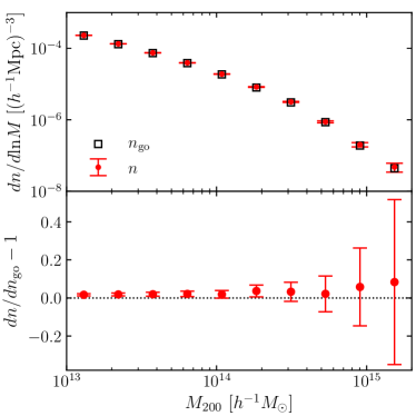
Figure 3.— Top panel compares the $z=0$ mass function of SO halos from the GO (black squares) and NR (red circles) Borg Cube simulations. Error bars denote the Poisson error in each mass bin and are shown only for the NR simulation in the upper panel for the purpose of clarity. The bottom panel shows the relative difference between the two simulations.

The interpretation is not that NR processes actually increase the number of massive halos, but rather the mass definition is altered by the internal redistribution of matter within individual halos. Since the two simulations use the same initial conditions, we are able to identify counterpart halos between each run and test this directly. Indeed, we find that halos in the NR run have $R_{200}$ that are $0.4\%$ larger on average than their GO counterparts; this equates to an average increase of $1\%$ in $M_{200}$. This number agrees well with the tSPH simulation of Cui et al. (2012) who confirm that changes in the NR mass function can be accounted for using a simple shift in mass. This will also hold true once cooling and feedback are considered though the change in halo mass will be much closer to the $10\%$ range (Stanek et al., 2009).

3.3. Baryon Fraction

We now shift gears to focus on the relative distribution of baryons and CDM within individual halos. The main quantity to explore is the global baryon mass fraction, $f_{b}\equiv M_{b,200}/M_{200}$, where $M_{b,200}$ is the baryon mass within a halo of total mass $M_{200}$. Figure 4 shows $f_{b}$ in units of the universal baryon fraction for five bins in halo mass at $z=0$. Red circles trace the median value in each bin for the NR run while error bars bracket the 25th and 75th percentiles. We find that halos of mass $M_{200}\geq$10^{13}\text{\,}\massh$$ have baryon fractions that are roughly about $95\%$ that of the cosmic mean. This lies slightly above the range of values ($f_{b}\approx 89\%-94\%$) reported in previous NR simulations (e.g., Ettori et al., 2006; Crain et al., 2007; Gottlöber & Yepes, 2007; Rudd et al., 2008; Stanek et al., 2010; Battaglia et al., 2013) for similar masses. Intrinsic scatter in this quantity has been shown to exist amongst hydro methods (Frenk et al., 1999; Kravtsov et al., 2005) with the trend that mesh-based codes tend to yield larger baryon fractions at the level of a few percent compared to tSPH. Hence, our results are more consistent with previous mesh-based results.

The physical mechanism responsible for depleting the baryon fraction below the cosmic mean is shock heating. As we will show later, this process tends to “puff out” baryons around $R_{200}$. This seems to be especially prominent for the lowest mass bin in Figure 4 where $f_{b}$ drops to a level of $91\%$. Note that Gonzalez et al. (2013) find a weak dependence of decreasing baryon fraction with decreasing $M_{500}$ in an observational study of a collection of galaxy clusters and groups. Unfortunately, testing this dependence with low-mass halos in the Borg Cube becomes difficult since we expect resolution issues to emerge at some point as we push to smaller scales. This issue is most readily examined with the GO run.

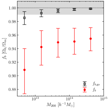
Figure 4.— Global baryon mass fractions in units of the universal mean computed for SO halos binned into five mass groups at $z=0$. Black squares and red circles show the median value in each bin for the GO and NR Borg Cube simulations, respectively. In each case, error bars bracket the 25th and 75th percentiles of the distribution. We naively expect the GO points to sit at unity and highlight $\pm 1\%$ deviations away from this using the shaded gray band. The departure of the GO result from unity indicates that the simulations are not converged for masses $M_{200}\lesssim$10^{13}\text{\,}\massh$$.

As mentioned earlier, coupling between unequal-mass CDM and baryon particles leads to artificially strong interactions on small scales. This will obviously impact the central depths of halos and will be more prominent in low-mass systems where physical scales are smaller and potential wells shallower. The black squares in Figure 4 trace the global baryon fractions from the GO simulation. Ideally, we expect these numbers to match the universal value since there is no distinction between CDM and baryon particles in the absence of hydro forces. This appears to be the case for masses $M_{200}\geq$10^{13}\text{\,}\massh$$ where $70\%$ of all halos are within $1\%$ of the cosmic mean. We see a clear trend of decreasing median and increasing scatter as we move from high- to low-mass systems. For instance, $67\%$ of halos with mass $M_{200}<$10^{13}\text{\,}\massh$$ have baryon fractions that deviate by more than $1\%$ from the universal value. Based on this, we set $M_{\rm con}=$10^{13}\text{\,}\massh$$ as the converged mass scale in the Borg Cube simulations. This is equivalent to roughly 3200 times the combined CDM and baryon particle mass. These findings agree well with the two-species GO simulations of Binney & Knebe (2002); Power et al. (2016) where halos containing fewer than a few thousand particles are also shown to exhibit a strong deficit of the low-mass group.

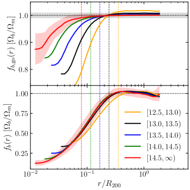
Figure 5.— The baryon fraction in radial shells normalized to the universal mean at $z=0$ for the Borg Cube GO (top panel) and NR (bottom panel) simulations. In each panel, the solid colored lines trace the stacked profiles for halos in five mass groups as indicated by the legend showing the log₁₀ ranges of each bin. Each profile is truncated below the gravitational softening length $r_{\rm soft}=$14\text{\,}\kpch$$. The shaded gray band in the top panel shows deviations of $\pm 1\%$ from unity, which we naively expect the GO result to reside. The shaded red band in each panel brackets the 25th and 75th percentiles of individual profiles for the highest mass bin. Vertical dotted lines denote the location of the physical scale $r_{\rm con}=$100\text{\,}\kpch$$ for the mass bin of the corresponding color.

We can investigate the issue of convergence further by looking at radial profiles of the baryon fraction. The top panel of Figure 5 shows this for the GO run where we overlay stacked profiles from the same set of five mass bins. We first note that the four converged mass bins are all within $1\%$ of the universal mean for $r\gtrsim 0.2R_{200}$. The lowest-mass bin, in contrast, shows a noticeably higher baryon fraction all the way out to $R_{200}$. In each case, as we move toward smaller radial bins, we find a sharp drop in baryon fraction until eventually hitting a plateau as we approach $r_{\rm soft}$. This sharp drop seems to occur at a constant physical scale of $r_{\rm con}=$100\text{\,}\kpch$$ as indicated by the vertical dotted lines showing where $r_{\rm con}$ intersects each mass bin. We attribute the precipitous drop in baryon fraction to artificially strong gravitational interactions within the central regions of halos leading to strong mass segregation (Efstathiou & Eastwood, 1981). Evidently, this process extends out to scales about seven times larger than the gravitational softening length. We conclude that individual baryon and CDM mass distributions in the GO run are converged down to $r_{\rm con}=$100\text{\,}\kpch$$. Recall that earlier we found the total matter distribution to be converged down to smaller scales of about $r_{m,{\rm con}}=$30\text{\,}\kpch$$ based on a comparison to the SS case (see Figure 1).

The bottom panel of Figure 5 shows analogous results from the NR simulation. In this case, the profiles from each of the four converged mass bins sit roughly on top of each other, suggesting a universal form for halos $M_{200}\geq$10^{13}\text{\,}\massh$$. It is unclear whether such a universal form extends to lower masses. In contrast to the GO run, we do not see any obvious features surfacing around the scale $r_{\rm con}$. The reason is that this scale is overwhelmed by thermal pressure support that naturally reduces baryon clustering, thus alleviating the problems encountered in the GO run. Hence, convergence criteria in the NR run are likely to be somewhat relaxed compared to the GO case. Note the same may not necessarily be true, for instance, in a hydrodynamic simulation with cooling processes that tend to promote baryon clustering on small scales, potentially exacerbating the issue further. While it is difficult to assess exactly to which scales the NR results are converged here, the smoothness and universality of the curves in Figure 5 down to $r_{\rm soft}$ are encouraging. We leave to future work a more detailed investigation of the numerical interplay between multi-species gravitational interactions and hydrodynamic processes.

3.4. Concentration

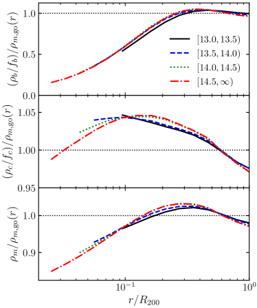
Figure 6.— Stacked radial density profiles of baryons (top), CDM (middle), and total matter (bottom) in the NR run relative to the GO total matter profile for each of the four converged mass bins at $z=0$. Curves are truncated below the total matter convergence scale of $r_{m,{\rm con}}=$30\text{\,}\kpch$$ for the GO run.

Next we explore the internal redistribution of matter that arises in response to shock heating. This complements the earlier analysis of the power spectrum which can be derived by integrating over the distribution of halo profiles via the halo model (e.g., Rudd et al., 2008). In Figure 6 we compare radial density profiles from the GO and NR runs stacked over all halos in each of the four converged mass bins. The top, middle, and bottom panels show density profiles for baryons, CDM, and total matter, respectively. In each case, we use the appropriately scaled total matter curve from the GO run as the comparison point and truncate each result below $r_{m,{\rm con}}$.

Figure 6 shows that changes in the individual species and total matter distributions are roughly consistent across all four mass bins. Unsurprisingly, baryons show the largest changes in the NR run with a slight enhancement in density at $r\approx 0.4R_{200}$ followed by a sharp drop that approaches one-tenth the density of the GO run at the halo center. Changes to the CDM show qualitatively similar trends with a slight depression at $R_{200}$ followed by an increase that peaks around $r\approx 0.2R_{200}$, and then a final small descent. Overall, the changes in CDM are quite minor being within $\pm 5\%$ of the GO result across the entire radial range. The total matter profile also starts with a small decrement at $R_{200}$ followed by an upturn that peaks at $r\approx 0.3R_{200}$ and finishes with a suppression that approaches $85\%$ of the GO density at the halo center. This result is consistent with the cumulative mass profiles from the modern SPH and mesh-based codes used in the nIFTy comparison project (Cui et al., 2016).

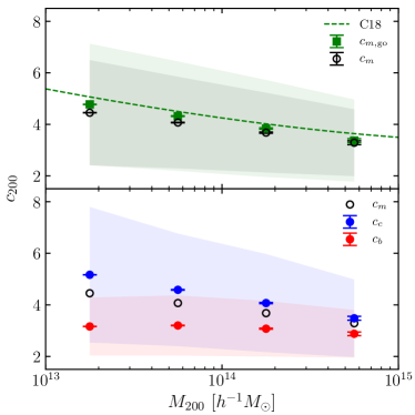
Figure 7.— Concentration-mass relation for all SO halos at $z=0$. Top panel compares $c_{200}$ based on the total matter profiles from the GO (green squares) and NR (black circles) Borg Cube runs. In each case, the data point shows the mean value of $c_{200}$ in each mass bin with the error bars denoting the standard error of the mean and the shaded region highlighting the standard deviation of the bin. The dashed green line traces the corresponding Child et al. (2018) fitting function. The bottom panel focuses on the individual baryon and CDM components from the NR run. Blue (red) circles follow the mean $c_{200}$ for CDM (baryons) with the black circles repeating the NR total matter relation from the top panel for comparison.

One way to summarize the redistribution of matter within halos is through the concentration. We plot the concentration-mass relation for all SO halos at $z=0$ in Figure 7 using the “peak finding” concentration method described earlier. The top panel shows $c_{200}$ computed from the total matter profiles for the GO and NR runs. For comparison, the dashed green line traces the Child et al. (2018) fitting function based on individual profiles for all (relaxed and unrelaxed) halos. This is in good agreement with the GO run which uses the same cosmology for which the fitting function was calibrated.

Comparing the total matter concentrations from the two runs shows a clear trend in a reduction of $c_{200}$ in the NR case. The difference is stronger at smaller masses with a $7\%$ reduction in the lowest mass bin and only a $2\%$ reduction in the highest mass bin. This disagrees with some earlier works (Rudd et al., 2008; Rasia et al., 2013) that find a $5-10\%$ increase in NR concentration over the same mass range. This discrepancy is not related to the definition of concentration since we find a similar level of reduction in $c_{200}$ when using concentrations based on fits to NFW profiles. Rather, the difference is likely sourced by a combination of two effects: 1) the earlier works were based on much smaller samples of halos with limited statistics; 2) the measurement of concentration is affected by the redistribution of baryons on small scales, which depends on the specific hydro solver, as evidenced in the measurements of power spectra in Figure 2.

The bottom panel of Figure 7 compares the concentrations from the baryon and CDM components of each SO halo in the NR run. As expected, baryon values are lower than CDM due to their shallow density profiles. Interestingly, the baryon result is nearly independent of mass with mean values $c_{200}\approx 3$ for each mass bin. CDM concentrations are markedly larger than baryons and display the usual trend of increasing $c_{200}$ with decreasing mass. Moreover, we find the CDM concentration in the NR run is larger than the GO total matter concentration at a level of $3\%$ for the highest mass bin and $8\%$ for the lowest mass bin. This reflects the earlier observations of increased small-scale CDM power (Figure 2) and enhanced density near the scale radius (middle panel of Figure 6).

While comparisons with earlier simulations are somewhat limited, this analysis shows that the predicted change in total matter concentration induced by NR processes depends on the details of the hydro solver. Of course, the inclusion of additional physics will significantly alter the density profiles and concentration-mass relations seen here. Cooling, on the one hand, increases concentration as baryons condense in the core while feedback, on the other hand, decreases concentration as matter is expelled from the inner to outer regions of a halo (Rasia et al., 2013; Shirasaki et al., 2018).

4. Gas Profiles

We have seen that NR processes significantly alter the internal structure of halos. We proceed here with a more complete description of the gaseous component of halos by measuring density, temperature, entropy, and pressure profiles over a wide range in mass. This analysis can be used in conjunction with analytic treatments like the halo model to construct a synthetic picture of the cosmological gas distribution. For this purpose, we also compare our results to a simple model based on the idea that gas exists in hydrostatic equilibrium (HSE) within the potential well of its host. Of course, such a description is only an idealized approximation since many halos are unrelaxed and therefore not in a state of equilibrium. In any event, it is useful to test the predictive power of HSE. In what follows, we work with the Komatsu & Seljak (2001) model based on the assumptions that baryons 1) trace the total matter density profile on halo outskirts, 2) follow a polytropic equation of state, and 3) exhibit full thermal pressure support. The first assumption is justified by the baryon fractions hovering around unity at $R_{200}$ in Figure 5 while the second assumption will be justified in Figure 8. We will explore the validity of the third assumption in the next section.

We begin with an overview of the HSE model compared to here. We point the interested reader to Komatsu & Seljak (2001) for a more careful derivation and also to Rabold & Teyssier (2017) who perform a similar analysis to our own. The starting point is based on the idea that the total matter distribution follows an NFW form:

$$\rho_{m}(x)=\frac{\rho_{s}}{cx(1+cx)^{2}},$$ (1)

where $x\equiv r/R_{200}$, $c$ is the concentration, and $\rho_{s}$ is a characteristic density set by the concentration:

$$\rho_{s}=\frac{c^{3}\rho_{200}}{3f(c)}.$$ (2)

Here $\rho_{200}$ is the overdensity criteria of the SO halo (i.e., 200 times the critical density) and

$$f(x)={\rm ln}(1+x)-\frac{x}{1+x}.$$ (3)

If we assume the baryons follow a polytropic equation of state, $P\propto\rho_{b}T\propto\rho_{b}^{\Gamma}$, with pressure $P$, temperature $T$, and polytropic index $\Gamma$, we can derive the density profile that results from HSE within an NFW potential:

$$\rho_{b}(x)=\rho_{0}\left[\frac{{\rm ln}(1+cx)}{cx}\right]^{{1}/({\Gamma-1})}.$$ (4)

Here $\rho_{0}$ is the asymptotic density approached at the halo center, and is constrained by requiring that the baryon density trace the total matter density at $R_{200}$. Setting $\rho_{b}(1)=f_{b}\rho_{m}(1)$ yields:

$$\rho_{0}=\frac{f_{b}\rho_{s}}{c(1+c)^{2}}\left[\frac{{\rm ln}(1+c)}{c}\right]^{{-1}/({\Gamma-1})}.$$ (5)

The temperature profile follows as:

$$T(x)=T_{0}\frac{{\rm ln}(1+cx)}{cx},$$ (6)

where the central temperature is derived from the requirement that the density profile drop to zero at infinity:

$$T_{0}=\frac{4\pi G\mu m_{p}\rho_{s}R_{200}^{2}}{k_{B}c^{2}}\frac{\Gamma-1}{\Gamma}.$$ (7)

Here $G$ is the gravitational constant, $k_{B}$ the Boltzmann constant, $\mu=0.59$ the mean molecular weight for a fully ionized gas, and $m_{p}$ the proton mass. Finally, the pressure follows as:

$$P(x)=\frac{\rho_{0}}{\mu m_{p}}k_{B}T_{0}\left[\frac{{\rm ln}(1+cx)}{cx}\right]^{{\Gamma}/({\Gamma-1})}.$$ (8)

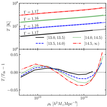
Figure 8.— Stacked temperature versus density profiles for each of the four SO halo mass bins in the NR run at $z=0$. Each of the lightly shaded solid lines in the top panel traces the linear regression performed on the mass bin of the corresponding color. Adding one to the slope of each line yields the polytropic index which ranges from $1.16-1.17$ for the different mass bins. The bottom panel shows the relative difference between the stacked profiles and the linear regression.

The preceding derivation has two free parameters: 1) the polytropic index and 2) the concentration of the total matter density profile. We compute the polytropic index by performing a linear regression on a log-log plot of temperature versus density. This is shown in Figure 8 for each of the four mass bins. The best-fit values of $\Gamma$ range from 1.16 to 1.17, which is similar to those found in earlier works (Komatsu & Seljak, 2001; Ascasibar et al., 2003; Rabold & Teyssier, 2017). Though the assumption that a single value of $\Gamma$ holds across the entire radial range is only an approximation (Kay et al., 2004; Battaglia et al., 2012b), the deviations seen here from the best-fit constant values are relatively small. The most noticeable difference shows up as an upturn in the $T-\rho_{b}$ relation at high density suggesting that larger values of $\Gamma$ may be more appropriate in the central regions where $r/R_{200}\lesssim 0.1$. For the sake of simplicity, we will use a constant value of $\Gamma=1.17$ for each of the mass bins in the following analysis.

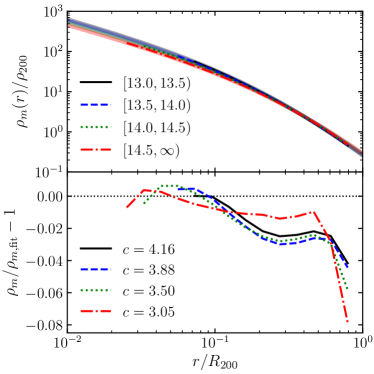
Figure 9.— Stacked total matter density profiles for each of the four SO halo mass bins in the NR run at $z=0$. Each stacked profile is truncated below twice the gravitational softening length and above $R_{200}$. The lightly shaded solid lines in the top panel trace the best-fit NFW profiles for the mass bin of the corresponding color. The bottom panel shows the relative difference between the stacked profiles and the NFW fit with the concentration of each mass bin listed in the legend.

We determine the NFW concentration of the total matter distribution by fitting equation (1) to the stacked density profile of each mass bin. The results are shown in Figure 9. When performing the fit, we avoid resolution issues by truncating the stacked density profile below twice the softening length, and also include only those radial bins up to $R_{200}$. Overall, an NFW profile does a relatively good job at describing the stacked total matter profiles with deviations within $3\%$ over most of the radial range. The deviations seem to get worse with increasing radial distance with the stacked profiles systematically falling off more steeply than an NFW form. This trend was also observed in Child et al. (2018), and is not surprising given that we are stacking over relatively wide mass bins. In any event, the deviations found here are relatively small, and we compute the best-fit NFW concentrations $c=3.05$, 3.50, 3.88, and 4.16 for the four bins in descending order of mass.

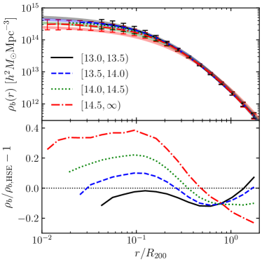
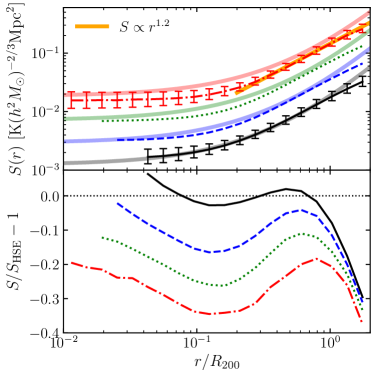
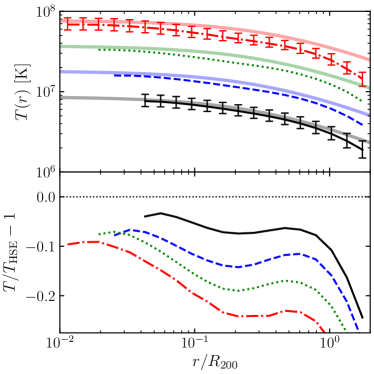
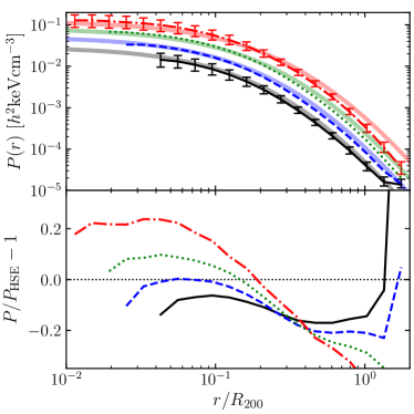
Figure 10.— Stacked profiles for density, temperature, pressure, and entropy in clockwise order from the top-left. Opaque lines in the upper panel of each plot show the NR result at $z=0$ with the profile for each mass bin truncated below the gravitational softening length. Stacks use the median value in each bin and we show the 25th and 75th percentiles of the highest (lowest) mass bin with red (black) error bars. The error bars do not depend strongly on mass and are thus only shown for the highest and lowest bins to avoid overcrowding the plots. The lightly shaded lines trace the HSE prediction for the mass bin of the corresponding color. The lower panel of each plot shows the relative difference between the simulation curves and the HSE model. The thick orange line in the entropy plot shows the $S\propto r^{1.2}$ power-law fit to the highest mass bin in the range $r>0.2R_{200}$.

Figure 10 shows stacked profiles for density, temperature, entropy, and thermal pressure for each of the four mass bins. The opaque lines in the upper panel of each plot trace the median value of the stacked profile while the red (black) error bars show the 25th and 75th percentiles of the highest (lowest) mass bin. The error bars are relatively insensitive to mass so we show them for only two mass bins to avoid overcrowding the plots. The lightly shaded lines show the HSE prediction of the mass bin of the corresponding color using a  constant $\Gamma=1.17$ and the best-fit NFW concentration from the total matter density profile. The lower panel in each plot shows the relative difference between the stacked profile and the HSE prediction.

We begin by looking at density in the top-left panel of Figure 10. In contrast to the cuspy NFW profiles typical of CDM, baryons asymptote to relatively flat central density cores for $r/R_{200}\lesssim 0.1$. This trend is consistent with that observed in mesh-based and modern SPH simulations (e.g., Frenk et al., 1999; Sembolini et al., 2016), and also arises naturally in the HSE model. The three lower-mass bins agree within $20\%$ of the HSE model for the entire radial range, while the highest-mass bin has maximum deviations occurring at the $40\%$ level. In general, it appears as though the HSE model becomes more inaccurate with increasing mass. This could reflect the fact that higher mass halos are more likely to be unrelaxed so that the assumption of HSE is less valid. The HSE curves all systematically underestimate the density at $R_{200}$, which follows from the trend in Figure 9 that the stacked profiles fall off steeper than NFW near the halo radius. The intersection of the four curves in the lower panel arises from the fact that both the simulated and model curves pass through each other around $r/R_{200}\approx 0.7$. Such a feature is expected from equation (4) which exhibits a pivot at $x=0.7$ with changing concentration.

The top-right panel in Figure 10 shows stacked temperature profiles. The separate mass bins show self-similar results with inwardly rising temperatures that approach a core value roughly three times greater than the value at $R_{200}$. Indeed, Loken et al. (2002) confirmed that a universal temperature profile arises within NR simulations. The HSE model does a good job at predicting the core temperature from the simulation, but heavily overestimates its value at $R_{200}$. A similar trend was noticed in Rabold & Teyssier (2017) who suggest a modification to equation (6) that accounts for contributions from turbulent pressure support. Their correction increases with radius and reduces the HSE prediction by about $6\%$ at $R_{200}$. Even without this correction, the HSE model does a relatively decent job at matching the simulation, being within about $30\%$ for $r<R_{200}$ in each mass bin. We will explore later the issue of non-thermal pressure support.

Next we examine entropy, which we define as $S\equiv T\rho_{b}^{-2/3}$. Entropy is a particularly useful quantity since it plays the fundamental role in shaping the density and temperature distributions. It also encapsulates the thermodynamic history of heating and cooling processes during structure formation (e.g., Voit, 2005). The simulation curves in the bottom-left panel of Figure 10 show self-similar behavior with inwardly decreasing entropy that approaches an isentropic core with a value about one-tenth that at $R_{200}$. Voit et al. (2005) showed that entropy profiles of NR halos follow a power-law with slope 1.2 for $r>0.2R_{200}$. We also recover this trend, as seen with the thick orange line comparing this power-law to the highest mass bin. Coincident with our previous results, the HSE model matches the low-mass bins quite well and stays within $40\%$ for all bins up to $R_{200}$. The systematic over-prediction of entropy for $r\gtrsim R_{200}$ follows from the breakdown of the assumption of full thermal pressure support. As shown in the next section, contributions from non-thermal pressure support increase with radius, possibly explaining the sharp drop-off in agreement between the simulation entropy and the HSE prediction seen in the highest radial bins.

Finally, the bottom-right panel of Figure 10 shows stacked thermal pressure profiles. As before, we see self-similar results across each mass bin with inwardly rising pressure that increases by almost three orders of magnitude in the central region compared to $R_{200}$. Self-similar cluster pressure profiles have previously been found in both simulations and observations (Nagai et al., 2007a; Arnaud et al., 2010). The simulation results agree within about $20\%$ of the HSE model for $r/R_{200}\leq 0.4$, but fall systematically below on larger scales. Again, this is a consequence of the fact that a significant fraction of pressure support on those scales is non-thermal. The flattening of the simulated pressure profiles for the two lower mass bins above $R_{200}$ is likely the result of contributions from the surrounding environment.

In summary, we find a great deal of self-similarity in the thermodynamic properties of the gas over a wide range in halo mass. This arises because the range in concentration seen here is rather small and NR processes are scale free. This trend will likely break down with the inclusion of more sophisticated gas treatments including cooling, star formation, and feedback which vary with halo mass. These processes most strongly impact the central regions of halos so the results presented here will be most applicable to halo outskirts. In fact, Burns et al. (2010) found that NR simulations are sufficient at matching the density, temperature, and entropy profiles of observed clusters on scales $r\gtrsim 0.5R_{200}$. Similar conclusions have been drawn by comparing NR simulations to those with additional physics (e.g., Loken et al., 2002; Roncarelli et al., 2006; Eckert et al., 2012; Planelles et al., 2014; Cui et al., 2016; Shirasaki et al., 2018).

5. Hydrostatic Masses and Non-thermal Pressure

The preceding analysis showed that the simple analytic model of Komatsu & Seljak (2001) was able to match the gas distribution of Borg Cube halos to within $40\%$ for halos spanning two orders of magnitude in mass. The largest discrepancies in the HSE model occurred close to $R_{200}$ and are at least partly explained by its omission of non-thermal pressure support, which we show later to be most important at large radial distance and high halo mass. The major contribution of non-thermal support is expected in the form of kinetic pressure from turbulent gas motions and bulk flows that generally increase with halo-centric radius. This accounts for $\approx 10-20\%$ of the total pressure support and leads to a bias of the same magnitude when deriving cluster masses based on HSE (Evrard, 1990; Kay et al., 2004; Faltenbacher et al., 2005; Rasia et al., 2006; Nagai et al., 2007b; Jeltema et al., 2008; Piffaretti & Valdarnini, 2008; Lau et al., 2009; Battaglia et al., 2012a; Nelson et al., 2012). Obviously, this is an important effect to understand and the large volume of the Borg Cube allows us to study its impact over a wide range in halo mass.

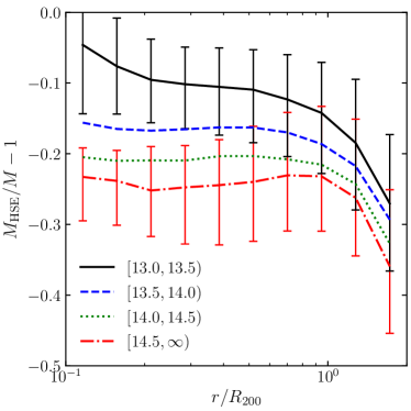
Figure 11.— Bias between the HSE mass estimate and simulation mass at $z=0$. Each line traces the median relation with the red (black) error bars showing the 25th and 75th percentiles of the highest (lowest) mass bin. We show the result down to only $0.1R_{200}$ as the relation becomes dominated by noise on smaller scales.

The assumption of HSE with spherical symmetry and full thermal pressure support can be used to estimate the mass of a galaxy cluster. The mass contained within radius $r$ is computed as:

$$M_{\rm HSE}(<r)=-\frac{k_{B}T(r)r}{G\mu m_{p}}\left[\frac{{\rm d\ ln}\rho_{b}(r)}{{\rm d\ ln}r}+\frac{{\rm d\ ln}T(r)}{{\rm d\ ln}r}\right].$$ (9)

We use this expression to compute a radial HSE mass estimate for each halo and compare this to the mass profile measured directly from the simulation. The resulting mass bias is shown in Figure 11. For the most massive bin, the HSE mass is biased low at a constant level of about $24\%$. This bias drops with decreasing halo mass with the mean bias in the radial range $[0.1-1]R_{200}$ being $21\%$, $17\%$, and $10\%$ for the three lower mass bins. These findings are in good agreement with the $\approx 20\%$ HSE mass biases for $M_{200}\gtrsim$10^{14}\text{\,}\massh$$ halos found in previous NR simulations (Kay et al., 2004; Nelson et al., 2012). Here we have assumed full information on both the density and temperature profiles in equation (9). Incomplete knowledge on either of these quantities has the potential to further bias the HSE estimate.

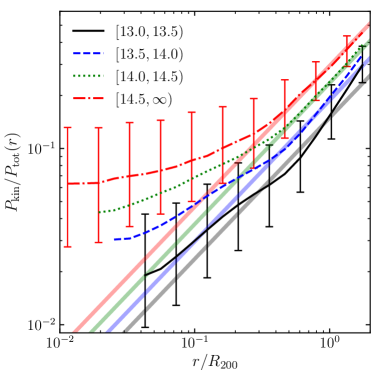
Figure 12.— Fraction of the kinetic pressure with respect to the total (kinetic plus thermal) pressure for each of the four mass bins in the NR run at $z=0$. The lighted shaded solid lines trace the fitting function from Battaglia et al. (2012a) which is based on power-law slopes of $4/5$ in radius and $1/5$ in mass. The fitting function is computed using the median halo mass in each bin. We show the 25th and 75th percentiles of the highest (lowest) mass bin as the red (black) error bars.

We can obtain a better understanding of the HSE mass bias by measuring the non-thermal pressure for each individual halo. Following Battaglia et al. (2012a), we focus here on bulk flows which should capture the major contribution to non-thermal support. We compute the corresponding kinetic pressure based on mass-averaged velocity fluctuations:

$$P_{\rm kin}=\frac{\rho_{b}}{3}\left\langle\delta v\cdot\delta v\right\rangle$$ (10)

The velocity fluctuations are made with respect to the baryon center of mass, $\mathrm{bar}{x}$, and mass-averaged velocity, $\mathrm{bar}{v}$, within $R_{200}$:

$$\delta v=a(v-\mathrm{bar}{v})+\dot{a}(x-\mathrm{bar}{x}).$$ (11)

The resulting kinetic pressure profiles are shown in Figure 12 as the fraction of the total pressure. These are compared to the fitting function from Battaglia et al. (2012a) which is based on the Shaw et al. (2010) power-law fitting function with an additional mass dependency that scales as $M_{200}^{1/5}$.

The fitting function does a good job at matching our simulation results for $r/R_{200}\gtrsim 0.4$, but dramatically underestimates the kinetic pressure on smaller scales. In this case, a broken power-law with a shallower slope on small scales would be more appropriate. We expect the NR results to be accurate for $r/R_{200}\gtrsim 0.1$ since bulk flows on these scales will be gravitationally sourced and mostly unaffected by cooling and feedback processes occurring on smaller scales (Battaglia et al., 2012a; Nelson et al., 2014). Indeed, the fitting function in Figure 12 was calibrated against simulations with cooling and feedback. Earlier works have shown that kinetic pressure is greater in less relaxed systems which have undergone recent major mergers (Jeltema et al., 2008; Piffaretti & Valdarnini, 2008; Lau et al., 2009; Nelson et al., 2014). The rise of the kinetic pressure fraction with increasing mass is consistent with the picture that high-mass systems are more likely to be unrelaxed and dynamically disturbed. This is also consistent with the previous finding that the mass bias is higher for more massive halos. Moreover, the large error bars demonstrate that a considerable amount of halo-to-halo scatter exists in the kinetic pressure fraction.

6. Sunyaev-Zel’dovich Effect

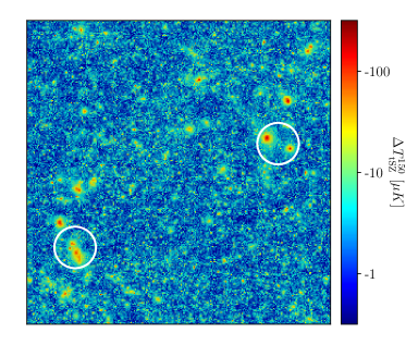
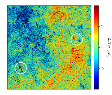
Figure 13.— tSZ (left) and kSZ (right) temperature fluctuations for a 7.3^∘$\times$7.3^∘ patch of the sky obtained by integrating through a particle lightcone from the NR Borg Cube run. The tSZ is shown at an observing frequency of $150\text{\,}\mathrm{GHz}$ where the signal is a decrement with respect to the CMB. Note the clear visibility of clusters in the tSZ map which correspond to hot and cold spots in the kSZ map. Also visible is the pairwise kSZ signal associated with nearby clusters. White circles in each image denote the location of two nearby clusters whose pairwise signal appears in the kSZ map.

CMB photons interact with matter during their passage between the surface of last scattering and today, resulting in a set of secondary anisotropies that overwhelm the primary CMB signal on small angular scales. The main contributor is the Sunyaev-Zel’dovich (SZ) effect which is usually separated into its thermal (tSZ) and kinematic (kSZ) components (Sunyaev & Zeldovich, 1970, 1972). The SZ effect is sourced by inverse Compton scattering off free electrons with the thermal component weighted towards hot cluster gas whereas the kinematic component is more sensitive to bulk flows. Hence, together the integrated tSZ and kSZ signals contain a wealth of information regarding the evolution of structure formation and the ionization state of the universe.

The magnitude of the thermal and kinematic components can be described in terms of the dimensionless Compton $y$ and Doppler $b$ parameters, respectively. The former involves an integration of electron pressure along the line-of-sight ($\hat{n}$):

$$y=\frac{\sigma_{T}}{m_{e}c^{2}}\int P_{e}(l)dl=\frac{\sigma_{T}k_{B}}{m_{e}c^{2}}\int n_{e}(l)T_{e}(l)dl,$$ (12)

while the latter involves an integration over the electron peculiar velocity:

$$b=-\frac{\sigma_{T}}{c}\int n_{e}(v_{e}\cdot\hat{n})dl.$$ (13)

Here $\sigma_{T}$ is the Thomson cross section, $k_{B}$ the Boltzmann constant, $m_{e}$ the electron mass, $c$ the speed of light, $n_{e}$ the free electron number density, $T_{e}$ the electron temperature, and $(v_{e}\cdot\hat{n})$ the electron peculiar velocity projected along the line-of-sight. We use the convention that $v_{e}>0$ for gas moving away from the observer. The electron number density is related to the gas density, $\rho_{g}$, via:

$$n_{e}=\frac{\chi\rho_{g}}{\mu_{e}m_{p}},$$ (14)

where $m_{p}$ is the proton mass and $\mu_{e}=1.14$. $\chi$ is the fraction of electrons that are ionized and is derived from the primordial helium abundance, $Y$, and the number of electrons ionized per helium atom, $N_{\rm He}$, as:

$$\chi=\frac{1-Y(1-N_{\rm He}/4)}{1-Y/2}.$$ (15)

This expression assumes that hydrogen is fully ionized. In what follows, we take $Y=0.24$ and assume that helium is neutral ($N_{\rm He}=0$) so that $\chi=0.86$. We also implicitly work in the non-relativistic regime.

The SZ temperature fluctuations about the CMB monopole are recovered from $y$ and $b$ as:

$$\frac{\Delta T}{T_{\rm CMB}}(\hat{n})=\frac{\Delta T_{\rm tSZ}}{T_{\rm CMB}}+\frac{\Delta T_{\rm kSZ}}{T_{\rm CMB}}=f_{\nu}y+b.$$ (16)

The function $f_{\nu}$ encapsulates the frequency dependence of the tSZ signal:

$$f_{\nu} \equiv x_{\nu}{\rm coth}(x_{\nu}/2)-4,$$

$$x_{\nu} \equiv h\nu/(k_{B}T_{\rm CMB}),$$ (17)

where $\nu$ is the observing frequency and $h$ is the Planck constant. The tSZ spectral dependence has a null at $\nu_{0}\approx$218\text{\,}\mathrm{GHz}$$ with temperature decrements (increments) occurring at frequencies less (greater) than $\nu_{0}$. The kSZ signal, in contrast, is independent of frequency for the non-relativistic case assumed here.

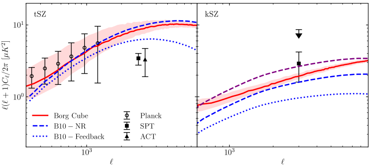
Figure 14.— Angular power spectra for tSZ at $150\text{\,}\mathrm{GHz}$ (left) and kSZ (right). The solid red lines trace the median result for power spectra computed in 83 independent maps of equal area $53.7\text{\,}\sqdeg$ while the shaded region shows the $1\sigma$ spread. The dashed (dotted) blue line traces the NR (feedback) simulation of Battaglia et al. (2010) which have been appropriately scaled to the Borg Cube cosmology (see text). Circles with error bars show the low-$\ell$ Planck tSZ measurements (Planck Collaboration et al., 2016) while squares and triangles show the $\ell=3000$ constraints from SPT (George et al., 2015) and ACT (Dunkley et al., 2013), respectively. The SPT and ACT tSZ constraints have been shifted horizontally for clarity. The ACT kSZ constraint corresponds to an upper limit. The dashed purple line in the right panel shows the Battaglia et al. (2010) NR kSZ result rescaled by the Shaw et al. (2012) correction of $67\%$ estimated to account for finite volume effects.

We generate synthetic $y$ and $b$ maps by integrating equations (12) and (13) through a particle lightcone covering one octant of the sky. In order to fill the entire volume, we stack the simulation box while applying random rotations to each replicant so as to avoid repeating the same structure along the line-of-sight. We compute the temperature of each baryon particle at the time of lightcone crossing by linearly interpolating its value at the two snapshots adjacent to the crossing. Velocities are computed from the difference in particle position at the two adjacent snapshots. We evaluate equation (12) from redshift $z=0.1$ to 5 using a total of 71 particle snapshots while equation (13) is evaluated from $z=0.1$ to 3 using 54 snapshots. In each case, the lower bound is chosen to remove large variance associated with the possibility of a massive cluster appearing in the field of view at low redshift. The $b$ map is integrated up to only $z=3$ since we found that the finite box size creates visually large velocity discontinuities along the boundaries of the stacked boxes. This issue becomes worse at higher redshift as the angle subtended by the box decreases; the angular extent of the box at $z=3$ is roughly $10^{\circ}$. This issue is much less apparent in the $y$ map since the density and temperature fields are relatively smooth on large scales, allowing us to integrate to higher redshift. The integrated $y$ and $b$ maps are then projected onto the sky using a HEALPIX (Górski et al., 2005) grid with $0.184\text{\,}\sqamin$ resolution ($N_{\rm side}=8192$). The lightcone is generated using all baryon particles for $z\leq 1$ while sampling at a rate of $50\%$ for $1<z\leq 2$, $25\%$ for $2<z\leq 3$, and $12.5\%$ for $z>3$.

Figure 13 shows $7.3^{\circ}$$\times$$7.3^{\circ}$ Cartesian projections of tSZ and kSZ temperature fluctuations from the NR run. The tSZ map is shown at frequency $\nu=$150\text{\,}\mathrm{GHz}$$ for consistency with SPT and ACT observations; at this frequency, temperature fluctuations are decrements with respect to the CMB. Since the tSZ signal is weighted toward hot intracluster gas, it is easy to visually pick out the strong temperature decrements associated with the cores of massive clusters. The location of these clusters also appear as hot and cold spots in the kSZ map. In addition, it is possible to see the presence of the pairwise kSZ signal associated with nearby clusters whose velocity vectors point in opposite directions along the line-of-sight, creating paired hot and cold spots (Flender et al., 2016). Note that this analysis involves only the post-reionization kSZ signal and thus ignores important contributions from the “patchy” network of ionized bubbles around luminous sources during the epoch of reionization. In general, the magnitude and shape of the patchy kSZ signal will depend on the duration of reionization and the size distribution of ionized bubbles (McQuinn et al., 2005; Zahn et al., 2005; Iliev et al., 2007).

We provide a more quantitative analysis by plotting the tSZ and kSZ angular power spectra in Figure 14. Power spectra are computed in 83 independent maps of equal area $53.7\text{\,}\sqdeg$ with the solid red line showing the median of these maps and the shaded region showing the $1\sigma$ scatter. For comparison, the dashed (dotted) blue line shows the NR (feedback) result from the simulations of Battaglia et al. (2010, hereafter B10). Circles with error bars show the low-$\ell$ Planck measurements (Planck Collaboration et al., 2016) while the squares and triangles show the $\ell=3000$ constraints from SPT (George et al., 2015) and ACT (Dunkley et al., 2013), respectively. In all cases, the tSZ power has been appropriately adjusted to $150\text{\,}\mathrm{GHz}$ using equation (17).

We find good agreement between the low-$\ell$ Planck tSZ measurements and the Borg Cube run. In contrast, our $\ell=3000$ power is considerably higher than the SPT and ACT constraints. This is expected given that our NR simulation does not include feedback which reduces gas pressure in cluster cores. This can be seen by comparing the NR and feedback simulations of B10. The agreement between the Borg Cube and B10 NR simulation is encouraging. There does appear to be a trend toward slightly smaller power at the highest $\ell$ in our run, which may reflect differences in the hydro solver (B10 use the tSPH scheme of GADGET). Of course, these scales will be highly sensitive to feedback processes. It is important to control for cosmology when comparing to other works since the tSZ effect is strongly cosmology dependent. We use the same $\sigma_{8}$ as B10, but have minor differences in baryon density, which we account for here by scaling the B10 result by $C_{\ell}\propto(\Omega_{b}h)^{2}$ (Komatsu & Seljak, 2002).

The kSZ signal has a significantly lower amplitude than its thermal counterpart. In our case, we find the $\ell=3000$ kSZ to be $22\%$ that of the $150\text{\,}\mathrm{GHz}$ tSZ signal. We again compare our result to the B10 NR run and adjust for cosmology using the $C_{\ell}\propto\Omega_{b}^{2.13}h^{1.68}z_{r}^{0.43}$ scaling relations suggested in Shaw et al. (2012). Here $z_{r}$ corresponds to the upper redshift limit which we take as $z_{r}=3$ while B10 use $z_{r}=10$. We find reasonable agreement between the Borg Cube and B10 NR curves though our result is systematically higher on all scales. One possibility for this discrepancy may be related to our larger simulation volume. Shaw et al. (2012) show that the truncation of large-scale velocity modes by finite simulation boxes can drastically underestimate the kSZ amplitude. They estimate a $67\%$ enhancement of kSZ power at $\ell=3000$ to compensate for the $165\text{\,}\Mpch$ box used in B10. In our case, an enhancement closer to $\approx 5\%$ would be more appropriate. The dashed purple line in Figure 14 shows the B10 NR result rescaled by a constant $67\%$. It is clear that finite volume effects have the potential to induce large changes on the simulated kSZ signal. Without comparing our result to a larger box, it is difficult to determine how much the discrepancies between our curves are driven by finite volume effects versus choices in the kSZ integration scheme or differences in the hydro solvers.

Our kSZ result at $\ell=3000$ is high compared to the SPT constraint given the fact that our analysis is missing power associated with integrating up to only $z=3$ and we additionally ignore contributions from patchy reionization . However, this high result would be partly offset by power suppression associated with feedback (as seen by comparing the B10 curves). Also recall that our analysis ignores power from free electrons associated with helium reionization which in principle would shift both our tSZ and kSZ curves up by a constant factor.

7. Summary

Constraining the nature of dark energy requires an accurate understanding of the impact of baryons on cosmological structure formation. This is a nontrivial task due to the high dynamic range of spatio-temporal scales involved and the complexities of the underlying astrophysics. Cosmological hydrodynamic simulations are the best option for modeling baryonic processes with high mass resolution in representative volumes. The simplest treatment involves NR physics where the thermal state of baryons changes only in response to gravitational shocks and the expansion of the universe. Even in this case, uncertainties arise due to systematics in the hydro solver. It is therefore crucial to compare the results from different codes in order to gauge the accuracy of predictions derived from simulations. This may also involve using the same code, but with different implementations (e.g., hydro solver, baryonic physics) so that changes between each comparison are minimized and systematics more easily isolated. The potential for systematics increases with the inclusion of subresolution physics treatments since a large degree of freedom exists in these models.

In this paper, we have presented results from the Borg Cube run which is the first cosmological hydrodynamic simulation based on the CRK-SPH formalism. We have restricted attention to the NR case since this provides the most parameter-free comparison point for hydro solvers. We have studied various statistics of the evolved matter field and drawn comparisons to previous simulations where available. We also compared the NR results to a GO version of the Borg Cube which used identical initial conditions. This is useful not only in showing the relative impact of shock heating, but also in identifying possible systematics that may arise from multi-species interactions. We report the main conclusions from these investigations in the following paragraphs.

Power spectra: the NR run shows a strong suppression (modest increase) of baryon (CDM) power on small scales relative to the GO case. This is in qualitative agreement with the earlier simulations of Jing et al. (2006) and Vogelsberger et al. (2014) which were based on tSPH and moving-mesh methods, respectively. The moving-mesh and CRK-SPH methods agree quite well on the details of baryon suppression at $z=0$ with $\approx 10\%$ suppression at $k\sim$1\text{\,}\invMpch$$ followed by a steep drop-off on scales $k\gtrsim$5\text{\,}\invMpch$$. In contrast, the tSPH result displays more modest suppression on the smallest scales. This likely owes to the fact that tSPH has been shown to over-shoot baryon clustering within the cores of collapsed objects (Frenk et al., 1999; Sembolini et al., 2016). The moving-mesh and CRK-SPH methods match very well in terms of CDM and total matter power with only few-percent differences emerging on scales $k\gtrsim$2\text{\,}\invMpch$$. Of course, it is precisely on such small scales where contributions from cooling and feedback lead to large changes compared to the NR case.

Matter redistribution within halos: shock heating induces an internal redistribution of both baryons and CDM within collapsed objects. We have shown that, relative to the GO case, this redistribution follows a roughly universal form independent of halo mass. To begin, both components exhibit a few-percent dip in density at $R_{200}$ relative to the GO run. For baryons, this is followed by an inward increase in relative density that peaks at a level of $5\%$ at $\approx 0.4R_{200}$ before sharply dropping to a value about one-tenth that of the GO run in the halo center. The CDM relative density also rises inward from $R_{200}$ and peaks at a $5\%$ enhancement while remaining near this level throughout most of the radial range. Since halos are defined with respect to a constant over-density, this redistribution leads to a systematic shift in the radius and mass of each SO halo. We find an average increase of $1\%$ in $M_{200}$ with a corresponding few-percent change in the mass function. These numbers agree well with the tSPH simulations of Cui et al. (2012). We can also describe these changes in terms of the concentration. We find that $c_{200}$ is reduced by $2\%$ ($7\%$) compared to the GO run for halos of mass $\sim$10^{15}~{}(10^{13})\text{\,}\massh$$. This is in contrast to the $5-10\%$ increase in $c_{200}$ found in earlier works (Rudd et al., 2008; Rasia et al., 2013); a discrepancy that is at least partly sourced by differences in hydro solvers.

Baryon fraction: we find the global baryon fraction within $R_{200}$ at $z=0$ to be about $95\%$ the universal mean for halos $M_{200}\geq$10^{13}\text{\,}\massh$$. Previous tSPH simulations find somewhat smaller values in the range $89-93\%$ (Ettori et al., 2006; Crain et al., 2007; Stanek et al., 2010; Battaglia et al., 2013) It has been shown that mesh-based methods produce baryon fractions $\approx 5\%$ higher than tSPH (Frenk et al., 1999; Kravtsov et al., 2005; Stanek et al., 2009); CRK-SPH also seems to fall within this camp. Likewise, the recent code comparison of Sembolini et al. (2016) showed that other modern SPH treatments produce baryon fractions more consistent with mesh-based codes.

Self-similar gas profiles: we find that stacked baryon density, temperature, entropy, and pressure profiles show self-similar results across all of the converged mass bins spanning two orders of magnitude in mass. The density profiles tend to cores within $0.1R_{200}$ with relatively constant concentrations $c_{200}\approx 3$. Temperature is found to slowly rise inward and approach a central value about three times larger than that at $R_{200}$. Entropy decreases inward with a power-law slope of 1.2 in radius before approaching an isentropic core within $0.1R_{200}$. Pressure rises strongly with decreasing radius reaching central values three orders of magnitude larger than at $R_{200}$. We attribute this self-similarity across mass to the fact that both the underlying NFW matter distribution and NR physics are relatively scale-free. This will not be the case when cooling and feedback prescriptions are included. As such, the NR results shown here are mostly applicable to halo outskirts for which $r\gtrsim 0.5R_{200}$. Indeed, Burns et al. (2010) confirm that NR simulations are sufficient at modeling observed cluster profiles on these scales.

Non-thermal pressure support: a simple model based on the assumption of HSE is capable of predicting density, temperature, entropy, and pressure within $40\%$ over two orders of magnitude in halo mass. In general, the model does not perform well around $R_{200}$ due to the breakdown of the assumption of full thermal pressure support. Similarly, observational estimates of cluster mass based on the assumption of HSE will be biased. The main contribution to non-thermal pressure comes from turbulent and bulk flows that develop during the structure formation process. Measuring this directly in the Borg Cube, we find $20-40\%$ of the total pressure support at $R_{200}$ comes from kinetic pressure. On average, this is higher for more massive halos with a power-law scaling of $1/5$ in $M_{200}$ as suggested in the feedback simulation of Battaglia et al. (2012a). The fraction of kinetic pressure drops with decreasing radius. We find HSE mass estimates are biased low by $24\%$ ($10\%$) for halos of mass $\sim$10^{15}~{}(10^{13})\text{\,}\massh$$. This is in agreement with previous NR simulations based on both tSPH and AMR methods (Kay et al., 2004; Nelson et al., 2012). The average bias does not evolve strongly within the radial range $[0.1-1]R_{200}$ though a considerable amount of halo-to-halo scatter ($10-15\%$) exists.

Sunyaev-Zel’dovich Effect: we compute angular power spectra for both the tSZ and kSZ effects by integrating through a particle lightcone from the Borg Cube run. Our NR results are most applicable to multipoles $\ell\lesssim 1000$ where we find good agreement with Planck tSZ measurements. Our tSZ result also shows excellent agreement with the NR simulation of B10 based on tSPH. This suggests that the tSZ signal derived from simulations is relatively insensitive to the choice of hydro solver. We find relatively good agreement with the B10 NR kSZ result though the comparison is difficult in this case since the small box of B10 is heavily impacted by artificial suppression of large-scale velocity modes. A comparison to a box of similar size as the Borg Cube would be needed to address how sensitive the simulated kSZ signal is to the choice of hydro solver. The Borg Cube SZ predictions at $\ell=3000$ are high compared to SPT and ACT constraints, which is expected given our omission of feedback.

Artificial particle coupling: special care must be taken to control numerical artifacts that may occur between particle species with unlike mass and/or initial power spectra. In both our GO and NR simulations, we employed a common approach of using a constant gravitational softening length for all particle pairs. It is easy to test for artifacts in the GO run since the CDM and baryons are effectively equivalent in this case. Artificial scattering between the heavy CDM and light baryons leads to an increase (decrease) in clustering for the former (latter) species. This is evident in individual power spectra as well as radial profiles of the baryon fraction. This issue propagated out to scales of about seven times the gravitational softening length in the GO run. The total matter distribution, on the other hand, was converged down to smaller scales of about twice the softening length suggesting that this process operates in such a way as to mostly preserve the total matter field. Furthermore, halos less massive than 3200 times the combined CDM plus baryon particle mass failed to converge in terms of the global baryon fraction. Isolating this effect is more difficult in the NR run and we did not see any clear systematics in radial profiles of the baryon fraction. It is plausible that the SPH smoothing kernel and artificial viscosity somewhat regulate the issue. We leave a more thorough investigation into the interplay between gravitational and hydrodynamic interactions to future work.

This work focused on the NR case and is thus valid on a limited range of scales. Including all the physics relevant to galaxy formation is a formidable challenge and one for which progress must be made in a controlled manner. On cosmological scales, the only path forward is through sub-resolution treatments of cooling and feedback. In this case, a large degree of modeling freedom exists and the potential for being systematics-limited increases. We use this work as the first stepping stone toward more sophisticated gas treatments within the CRK-HACC formalism.

References

- Almgren et al. (2013) Almgren, A. S., Bell, J. B., Lijewski, M. J., Lukić, Z., & Van Andel, E. 2013, ApJ, 765, 39
- Angulo et al. (2013) Angulo, R. E., Hahn, O., & Abel, T. 2013, MNRAS, 434, 1756
- Arnaud et al. (2010) Arnaud, M., Pratt, G. W., Piffaretti, R., et al. 2010, A&A, 517, A92
- Ascasibar et al. (2003) Ascasibar, Y., Yepes, G., Müller, V., & Gottlöber, S. 2003, MNRAS, 346, 731
- Bate & Burkert (1997) Bate, M. R., & Burkert, A. 1997, MNRAS, 288, 1060
- Battaglia et al. (2012a) Battaglia, N., Bond, J. R., Pfrommer, C., & Sievers, J. L. 2012a, ApJ, 758, 74
- Battaglia et al. (2012b) —. 2012b, ApJ, 758, 75
- Battaglia et al. (2013) —. 2013, ApJ, 777, 123
- Battaglia et al. (2010) Battaglia, N., Bond, J. R., Pfrommer, C., Sievers, J. L., & Sijacki, D. 2010, ApJ, 725, 91
- Binney & Knebe (2002) Binney, J., & Knebe, A. 2002, MNRAS, 333, 378
- Bryan et al. (2014) Bryan, G. L., Norman, M. L., O’Shea, B. W., et al. 2014, ApJS, 211, 19
- Burns et al. (2010) Burns, J. O., Skillman, S. W., & O’Shea, B. W. 2010, ApJ, 721, 1105
- Child et al. (2018) Child, H. L., Habib, S., Heitmann, K., et al. 2018, ArXiv e-prints, arXiv:1804.10199
- Crain et al. (2007) Crain, R. A., Eke, V. R., Frenk, C. S., et al. 2007, MNRAS, 377, 41
- Cui et al. (2012) Cui, W., Borgani, S., Dolag, K., Murante, G., & Tornatore, L. 2012, MNRAS, 423, 2279
- Cui et al. (2016) Cui, W., Power, C., Knebe, A., et al. 2016, MNRAS, 458, 4052
- Dawson et al. (2013) Dawson, K. S., Schlegel, D. J., Ahn, C. P., et al. 2013, AJ, 145, 10
- Dunkley et al. (2013) Dunkley, J., Calabrese, E., Sievers, J., et al. 2013, J. Cosmology Astropart. Phys, 7, 025
- Eckert et al. (2012) Eckert, D., Vazza, F., Ettori, S., et al. 2012, A&A, 541, A57
- Efstathiou & Eastwood (1981) Efstathiou, G., & Eastwood, J. W. 1981, MNRAS, 194, 503
- Ettori et al. (2006) Ettori, S., Dolag, K., Borgani, S., & Murante, G. 2006, MNRAS, 365, 1021
- Evrard (1990) Evrard, A. E. 1990, ApJ, 363, 349
- Faltenbacher et al. (2005) Faltenbacher, A., Kravtsov, A. V., Nagai, D., & Gottlöber, S. 2005, MNRAS, 358, 139
- Flender et al. (2016) Flender, S., Bleem, L., Finkel, H., et al. 2016, ApJ, 823, 98
- Frenk et al. (1999) Frenk, C. S., White, S. D. M., Bode, P., et al. 1999, ApJ, 525, 554
- Frontiere et al. (in prep.) Frontiere, N., Emberson, J. D., Habib, S., & Heitmann, K. in prep.
- Frontiere et al. (2017) Frontiere, N., Raskin, C. D., & Owen, J. M. 2017, Journal of Computational Physics, 332, 160
- George et al. (2015) George, E. M., Reichardt, C. L., Aird, K. A., et al. 2015, ApJ, 799, 177
- Gonzalez et al. (2013) Gonzalez, A. H., Sivanandam, S., Zabludoff, A. I., & Zaritsky, D. 2013, ApJ, 778, 14
- Górski et al. (2005) Górski, K. M., Hivon, E., Banday, A. J., et al. 2005, ApJ, 622, 759
- Gottlöber & Yepes (2007) Gottlöber, S., & Yepes, G. 2007, ApJ, 664, 117
- Habib et al. (2016) Habib, S., Pope, A., Finkel, H., et al. 2016, New A, 42, 49
- Heitmann et al. (2015) Heitmann, K., Frontiere, N., Sewell, C., et al. 2015, ApJS, 219, 34
- Heitmann et al. (2016) Heitmann, K., Bingham, D., Lawrence, E., et al. 2016, ApJ, 820, 108
- Hopkins (2015) Hopkins, P. F. 2015, MNRAS, 450, 53
- Hopkins et al. (2018) Hopkins, P. F., Wetzel, A., Kereš, D., et al. 2018, MNRAS, 480, 800
- Iliev et al. (2007) Iliev, I. T., Pen, U.-L., Bond, J. R., Mellema, G., & Shapiro, P. R. 2007, ApJ, 660, 933
- Jeltema et al. (2008) Jeltema, T. E., Hallman, E. J., Burns, J. O., & Motl, P. M. 2008, ApJ, 681, 167
- Jing et al. (2006) Jing, Y. P., Zhang, P., Lin, W. P., Gao, L., & Springel, V. 2006, ApJ, 640, L119
- Kay et al. (2004) Kay, S. T., Thomas, P. A., Jenkins, A., & Pearce, F. R. 2004, MNRAS, 355, 1091
- Komatsu & Seljak (2001) Komatsu, E., & Seljak, U. 2001, MNRAS, 327, 1353
- Komatsu & Seljak (2002) —. 2002, MNRAS, 336, 1256
- Komatsu et al. (2011) Komatsu, E., Smith, K. M., Dunkley, J., et al. 2011, ApJS, 192, 18
- Kravtsov et al. (1997) Kravtsov, A. V., Klypin, A. A., & Khokhlov, A. M. 1997, ApJS, 111, 73
- Kravtsov et al. (2005) Kravtsov, A. V., Nagai, D., & Vikhlinin, A. A. 2005, ApJ, 625, 588
- Lau et al. (2009) Lau, E. T., Kravtsov, A. V., & Nagai, D. 2009, ApJ, 705, 1129
- Laureijs et al. (2011) Laureijs, R., Amiaux, J., Arduini, S., et al. 2011, ArXiv e-prints, arXiv:1110.3193
- Levi et al. (2013) Levi, M., Bebek, C., Beers, T., et al. 2013, ArXiv e-prints, arXiv:1308.0847
- Lewis et al. (2000) Lewis, A., Challinor, A., & Lasenby, A. 2000, ApJ, 538, 473
- Lin et al. (2006) Lin, W. P., Jing, Y. P., Mao, S., Gao, L., & McCarthy, I. G. 2006, ApJ, 651, 636
- Loken et al. (2002) Loken, C., Norman, M. L., Nelson, E., et al. 2002, ApJ, 579, 571
- LSST Science Collaboration et al. (2009) LSST Science Collaboration, Abell, P. A., Allison, J., et al. 2009, ArXiv e-prints, arXiv:0912.0201
- McCarthy et al. (2007) McCarthy, I. G., Bower, R. G., Balogh, M. L., et al. 2007, MNRAS, 376, 497
- McQuinn et al. (2005) McQuinn, M., Furlanetto, S. R., Hernquist, L., Zahn, O., & Zaldarriaga, M. 2005, ApJ, 630, 643
- Melott (2007) Melott, A. L. 2007, arXiv:0709.0745
- Nagai et al. (2007a) Nagai, D., Kravtsov, A. V., & Vikhlinin, A. 2007a, ApJ, 668, 1
- Nagai et al. (2007b) Nagai, D., Vikhlinin, A., & Kravtsov, A. V. 2007b, ApJ, 655, 98
- Navarro et al. (1997) Navarro, J. F., Frenk, C. S., & White, S. D. M. 1997, ApJ, 490, 493
- Nelson et al. (2014) Nelson, K., Lau, E. T., & Nagai, D. 2014, ApJ, 792, 25
- Nelson et al. (2012) Nelson, K., Rudd, D. H., Shaw, L., & Nagai, D. 2012, ApJ, 751, 121
- Perlmutter et al. (1999) Perlmutter, S., Aldering, G., Goldhaber, G., et al. 1999, ApJ, 517, 565
- Piffaretti & Valdarnini (2008) Piffaretti, R., & Valdarnini, R. 2008, A&A, 491, 71
- Planck Collaboration et al. (2014) Planck Collaboration, Ade, P. A. R., Aghanim, N., et al. 2014, A&A, 571, A1
- Planck Collaboration et al. (2016) Planck Collaboration, Aghanim, N., Arnaud, M., et al. 2016, A&A, 594, A22
- Planelles et al. (2014) Planelles, S., Borgani, S., Fabjan, D., et al. 2014, MNRAS, 438, 195
- Power et al. (2003) Power, C., Navarro, J. F., Jenkins, A., et al. 2003, MNRAS, 338, 14
- Power et al. (2016) Power, C., Robotham, A. S. G., Obreschkow, D., Hobbs, A., & Lewis, G. F. 2016, MNRAS, 462, 474
- Rabold & Teyssier (2017) Rabold, M., & Teyssier, R. 2017, MNRAS, 467, 3188
- Rasia et al. (2013) Rasia, E., Borgani, S., Ettori, S., Mazzotta, P., & Meneghetti, M. 2013, ApJ, 776, 39
- Rasia et al. (2004) Rasia, E., Tormen, G., & Moscardini, L. 2004, MNRAS, 351, 237
- Rasia et al. (2006) Rasia, E., Ettori, S., Moscardini, L., et al. 2006, MNRAS, 369, 2013
- Raskin & Owen (2016) Raskin, C., & Owen, J. M. 2016, ApJ, 831, 26
- Riess et al. (1998) Riess, A. G., Filippenko, A. V., Challis, P., et al. 1998, AJ, 116, 1009
- Roncarelli et al. (2006) Roncarelli, M., Ettori, S., Dolag, K., et al. 2006, MNRAS, 373, 1339
- Rudd et al. (2008) Rudd, D. H., Zentner, A. R., & Kravtsov, A. V. 2008, ApJ, 672, 19
- Saitoh et al. (2008) Saitoh, T. R., Daisaka, H., Kokubo, E., et al. 2008, PASJ, 60, 667
- Sembolini et al. (2016) Sembolini, F., Yepes, G., Pearce, F. R., et al. 2016, MNRAS, 457, 4063
- Shaw et al. (2010) Shaw, L. D., Nagai, D., Bhattacharya, S., & Lau, E. T. 2010, ApJ, 725, 1452
- Shaw et al. (2012) Shaw, L. D., Rudd, D. H., & Nagai, D. 2012, ApJ, 756, 15
- Shirasaki et al. (2018) Shirasaki, M., Lau, E. T., & Nagai, D. 2018, MNRAS, 477, 2804
- Spergel et al. (2013) Spergel, D., Gehrels, N., Breckinridge, J., et al. 2013, ArXiv e-prints, arXiv:1305.5422
- Springel (2005) Springel, V. 2005, MNRAS, 364, 1105
- Springel (2010) —. 2010, MNRAS, 401, 791
- Springel et al. (2018) Springel, V., Pakmor, R., Pillepich, A., et al. 2018, MNRAS, 475, 676
- Stanek et al. (2010) Stanek, R., Rasia, E., Evrard, A. E., Pearce, F., & Gazzola, L. 2010, ApJ, 715, 1508
- Stanek et al. (2009) Stanek, R., Rudd, D., & Evrard, A. E. 2009, MNRAS, 394, L11
- Sunyaev & Zeldovich (1970) Sunyaev, R. A., & Zeldovich, Y. B. 1970, Ap&SS, 7, 3
- Sunyaev & Zeldovich (1972) —. 1972, Comments on Astrophysics and Space Physics, 4, 173
- Teyssier (2002) Teyssier, R. 2002, A&A, 385, 337
- The Dark Energy Survey Collaboration (2005) The Dark Energy Survey Collaboration. 2005, ArXiv Astrophysics e-prints, astro-ph/0510346
- Valkenburg & Villaescusa-Navarro (2017) Valkenburg, W., & Villaescusa-Navarro, F. 2017, MNRAS, 467, 4401
- Villaescusa-Navarro et al. (2017) Villaescusa-Navarro, F., Banerjee, A., Dalal, N., et al. 2017, ArXiv e-prints, arXiv:1708.01154
- Vogelsberger et al. (2014) Vogelsberger, M., Genel, S., Springel, V., et al. 2014, MNRAS, 444, 1518
- Voit (2005) Voit, G. M. 2005, Reviews of Modern Physics, 77, 207
- Voit et al. (2005) Voit, G. M., Kay, S. T., & Bryan, G. L. 2005, MNRAS, 364, 909
- Wadsley et al. (2017) Wadsley, J. W., Keller, B. W., & Quinn, T. R. 2017, MNRAS, 471, 2357
- Weinberg et al. (2013) Weinberg, D. H., Mortonson, M. J., Eisenstein, D. J., et al. 2013, Phys. Rep., 530, 87
- Yoshida et al. (2003) Yoshida, N., Sugiyama, N., & Hernquist, L. 2003, MNRAS, 344, 481
- Zahn et al. (2005) Zahn, O., Zaldarriaga, M., Hernquist, L., & McQuinn, M. 2005, ApJ, 630, 657
- Zel’dovich (1970) Zel’dovich, Y. B. 1970, A&A, 5, 84