Thermodynamics at Strong Coupling
on Anisotropic Lattices

Abstract:

Lattice QCD with staggered fermions at strong coupling has long been studied in a dual representation to circumvent the finite baryon density sign problem. Monte Carlo simulations at finite temperature and density require anisotropic lattices. Recent results that established the non-perturbative functional dependence between the bare anisotropy $\gamma$ and the physical anisotropy $a_{s}/a_{t}$ in the chiral limit are now extended to finite quark mass. We illustrate how the calibration of the anisotropy works and discuss the consequences of the anisotropy on thermodynamic observables. We also show first results on the energy density and pressure in the QCD phase diagram in the strong coupling regime.

1 Introduction: Sign Problem

Lattice QCD at finite baryon density suffers from the numerical sign problem: no direct simulations based on the fermion determinant (such as RHMC) are feasible, due to the fact that the fermion determinant becomes complex for $\mu_{B}>0$. Hence, with the well established methods, a possible critical endpoint is still out of reach. Methods based on a complexified parameter space (Complex Langevin, Lefschetz Thimbles) are promising, but not (yet) applicable to full QCD. Since the sign problem is representation-dependent, the partition sum can also be rewritten in new degrees of freedom which are closer to the physical states. Then the sign problem can be milder or even be absent. Here, we will make use of so-called dual representations,. These have been proven useful in many models which have severe sign problems in the original formulation (e. g. [1]). For lattice QCD, a dual representation is well known in the strong coupling limit in terms of a monomer-dimer system [2, 3, 4]. In this limit $\beta=\frac{2N_{c}}{g^{2}}\rightarrow 0$, it is possible to reverse the order of integration and integrate out all gauge fields $U_{\mu}(x)$ before the Grassman variables since link integration factorizes due to the absence of the plaquette contributions of the gauge action. The resulting color singlet degrees of freedom are mesons and baryons. This system has been studied since decades both via Monte Carlo and mean field and has proven to be a great laboratory for finite density QCD. The advantage of the dual formulation of strong coupling LQCD is twofold: (1) the very mild sign problem (which is even absent in the continuous time limit) and (2) the applicability of Worm algorithms that enable fast simulations. This allows to study the full phase diagram in the $\mu_{B}$ - $T$ plane.

2 The Dual Representation of Strong Coupling Lattice QCD

The strong coupling partition function is obtained from the fermionic action of staggered fermions by an exact rewriting of the path integral by integrating out the gluons first. Followed by Grassmann integration, it can be mapped on a discrete system of monomers $n_{x}\in\{0,\ldots N_{c}\}$, dimers $k_{b}\in\{0,\ldots N_{c}\}$, and world lines $\ell_{b}\in\{0,\pm 1\}$ [2, 3]:

$$Z_{F}(m_{q},\mu)=\sum_{\{k,n,\ell\}}\prod_{b=(x,\mu)}\frac{(N_{c}-k_{b})!}{N_{c}!k_{b}!}\prod_{x}\frac{N_{c}!}{n_{x}!}(2am_{q})^{n_{x}}\prod_{\ell}\left(\frac{1}{N_{c}!^{|\ell|}}\sigma(\ell)e^{3N_{t}r_{l}a_{\tau}\mu}\right)$$ (1)

The Grassmann integration imposes the following constraint on the sum over configurations in the above partition sum:

$$n_{x}+\sum_{\hat{\mu}=\pm\hat{0},\ldots\pm\hat{d}}\left(k_{\hat{\mu}}(x)+\frac{N_{c}}{2}|\ell_{\hat{\mu}}(x)|\right)=N_{c},$$ (2)

which is a remnant of the gauge group and entails that mesonic degrees of freedom (monomers and dimers) do not touch baryon world lines, The latter form oriented self-avoiding loops $\ell$ of length $|\ell|$, and its sign $\sigma(\ell)\in\{-1,+1\}$ depends on loop geometry.

The caveat of this formulation is that the lattice is very coarse, and it requires $\beta>0$ to make the lattice finer. In principle it is possible to include the effects of the gauge action by expanding it in terms of plaquette occupation numbers before integrating out the gauge links. This gives rise to a strong coupling expansion. Here, we do not include such corrections, but they have been addressed to next to leading order [5, 6] and have also been presented at this conference in the contribution [7] “Towards a Dual Representation of Lattice QCD” by G. Gagliardi. Alternative strategies with dual variables have been proposed in [8, 9]. The leading order gauge correction $\mathcal{O}(\beta)$ to the SC-LQCD phase diagram in the chiral limit has been first addressed via reweighting in $\beta$ from the ensemble at $\beta=0$ [5]. Here it was found that although the nuclear liquid gas critical end point splits from the chiral tri-critical point, the first order line from the nuclear transition and the chiral transition did not split. An immediate question one can ask is: do the nuclear and chiral transition split at sufficiently large $\beta$? New simulations obtained by sampling plaquette contributions directly via world sheets did not indicate any splitting [6]. We may have to consider the possibility that in the chiral limit, both transitions are on top even in the continuum limit. Hence it might be necessary to address simulations at finite quark mass for the splitting to be sizeable. This motivates the study presented here.

3 Thermodynamics of Strong Coupling Lattice QCD

In order to vary the temperature in the strong coupling limit, where the lattice spacing $a(\beta)$ cannot be modified at fixed $\beta=0$, we need to introduce the bare anisotropy $\gamma$ in the Dirac couplings. This is in particular necessary since $aT=1/N_{t}$ is discrete (with $N_{t}$ even): it turns out that the chiral transition temperature is about $aT_{c}\simeq 1.5$, hence we cannot address the phase transition on isotropic lattices. The bare anisotropy will change the temporal lattice spacing $a_{t}$ continuously at fixed $a_{s}\equiv a$. :

$$\mathcal{L}_{\rm F}(\hat{m},a_{t}\mu,\gamma) =\sum_{x}\left\{\sum_{\nu}\gamma^{\delta_{\nu 0}}\eta_{\nu}(x)\left(e^{a_{t}\mu\delta_{\nu 0}}\bar{\psi}_{x}U_{\nu}(x)\psi_{x+{\hat{\nu}}}-e^{-a_{t}\mu\delta_{\nu 0}}\bar{\psi}_{x+{\hat{\nu}}}U_{\nu}^{\dagger}(x)\psi_{x}\right)+2\hat{m}\bar{\psi}_{x}\psi_{x}\right\}$$

$$Z_{F}(\hat{m},a_{t}\mu,\gamma) =\sum\limits_{\{k,n,\ell\}}\prod\limits_{b=(x,\nu)}\frac{(N_{c}-k_{b})!}{N_{c}!k_{b}!}\gamma^{2k_{b}\delta_{\nu 0}}\prod\limits_{x}\frac{N_{c}!}{n_{x}!}(2\hat{m})^{n_{x}}\prod\limits_{\ell}w(\ell,a_{t}\mu)$$ (3)

The anisotropy $\frac{a_{s}}{a_{t}}\equiv\xi(\gamma)$ is a non-perturbative function of the bare anisotropy $\gamma$ which allows to define the temperature $aT=\frac{\xi(\gamma)}{N_{t}}$. At weak coupling one expects $\xi(\gamma)=\gamma$, however, at strong coupling, where the degrees of freedom are not quarks but hadrons, this is not the case. Mean field theory at strong coupling implies $\xi(\gamma)=\gamma^{2}$, since the square of the critical bare coupling is proportional to $N_{t}$: $\gamma_{c}^{2}=N_{t}\frac{(d-1)(N_{c}+1)(N_{c}+2)}{6(N_{c}+3)}$ [10]. However, modifications are expected beyond mean field, hence we need to determine the precise correspondence between $\xi\equiv a_{s}/a_{t}$ and $\gamma$.

Consider the SU(3) partition function Eq. (3), in terms of the extensive quantities: $N_{M}=\sum\limits_{x}n_{x}$ the total monomer number, $N_{q}=2N_{Dt}+3N_{Bt}$ (with $N_{Dt}=\sum\limits_{x}k_{x,0}$ and $N_{Bt}=\sum\limits_{x}|b_{x,0}|$ the total number of temporal dimer and temporal baryon segments), and $\Omega$ the total winding number of all baryon world lines. The dimensionless thermodynamic observables in terms of these dual variables are:

baryon density: $$a_{s}^{3}\rho_{B} =\left.a_{s}^{3}\frac{T}{V}\frac{\partial\log Z}{\partial\mu_{B}}\right|_{V,T}=\frac{\left\langle\Omega\right\rangle}{N_{\sigma}^{3}}=\left\langle\omega\right\rangle$$ (4)

energy density: $$a_{s}^{3}a_{t}\epsilon =\mu_{B}\rho_{B}-\left.\frac{a^{3}a_{t}}{V}\frac{\partial\log Z}{\partial T^{-1}}\right|_{V,\mu_{B}}=\frac{\xi}{\gamma}\frac{d\gamma}{d\xi}\left\langle n_{q}\right\rangle-\left\langle n_{M}\right\rangle$$ (5)

pressure: $$a_{s}^{3}a_{t}p =-\left.a_{s}^{3}a_{t}T\frac{\partial\log Z}{\partial V}\right|_{T,\mu_{B}}=\frac{\xi}{3\gamma}\frac{d\gamma}{d\xi}\left\langle n_{q}\right\rangle$$ (6)

.

chiral condensate: $$a_{s}^{4}\left\langle\bar{\psi}\psi\right\rangle =a_{s}^{4}\frac{\left\langle N_{M}\right\rangle}{N_{\sigma}^{3}N_{t}a_{s}^{4}a_{t}}=\frac{\xi}{\hat{m}}\left\langle n_{M}\right\rangle$$ (7)

interaction measure: $$\epsilon-3p =-\frac{\left\langle n_{M}\right\rangle}{a_{s}^{3}a_{t}}=-m_{q}\left\langle\bar{\psi}\psi\right\rangle$$ (8)

Clearly, most of these observables explicitly depend on $\xi(\gamma)$ and its derivative. They have been measured in the full $\mu_{B}$ - $T$ plane after having determined $\xi(\gamma)$ non-perturbatively.

4 Anisotropy Calibration and Results

The determination of $\xi(\gamma)$ in the chiral limit has already been addressed in [11, 12]. The non-perturbative result deviates from the mean field assignment $\xi_{\rm mf}(\gamma)=\gamma^{2}$ considerably:

$$\xi(\gamma) \approx\kappa\gamma^{2}+\frac{\gamma^{2}}{1+\lambda\gamma^{4}}\qquad\text{with}\qquad\kappa=0.781(1)$$ (9)

As an application, the dependence of observables on the anisotropy was studied: the pion decay constant, the chiral condensate and the baryon mass. With this result, it is also possible to define unambiguously the continuous time limit $a_{t}\rightarrow 0$ via $N_{t}\rightarrow\infty$ and $\gamma\rightarrow\infty$ at fixed $aT$, which is further elaborated in [13] and in a contribution to this conference “Temporal Correlators in the Continuous Time Limit of Lattice QCD” my M. Klegrewe [14]. The anisotropy calibration can also directly be performed in the continuous time limit.

In this proceedings, we want to extend these results to finite quark, i. e. we address the anisotropy calibration and its difficulties for $m_{q}>0$. In order to determine $\xi(\gamma)$ the idea is to consider the following current that is implied by the Grassmann constraint [15]:

$$j_{\mu}(x) =\sigma(x)\left(k_{\mu}(x)-\frac{N_{c}}{2}|b_{x,\mu}|-\frac{N_{c}}{2d}\right)\quad\rightarrow\quad\sum\limits_{\pm{\hat{\mu}}}(j_{\mu}(x)-j_{\mu}(x-{\hat{\mu}}))=-\sigma(x)n(x)$$ (10)

In the chiral limit, where $n(x)=0$, the current $j_{\mu}(x)$ is locally conserved. The conserved charge $Q_{\mu}=\sum\limits_{x\perp\mu}j_{\mu}(x)$ has $\left\langle Q_{\mu}\right\rangle=0$, but non-zero variance: $\left\langle Q_{\mu}^{2}\right\rangle\neq 0$. The calibration of $\xi(\gamma)$ is then obtained via a renormalization condition on demanding a physically isotropic box:

$$a_{t}N_{t} =a_{s}N_{s}\quad\Leftrightarrow\quad\left\langle Q_{t}^{2}\right\rangle(\gamma_{0})\stackrel{{\scriptstyle!}}{{=}}\left\langle Q_{s}^{2}\right\rangle(\gamma_{0}),\qquad\frac{a_{s}}{a_{t}}=\frac{N_{t}}{N_{s}}=\xi(\gamma_{0}).$$ (11)

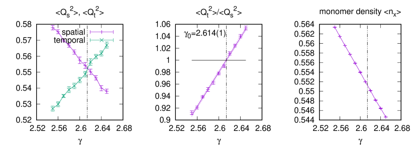
Figure 1: Anisotropy calibration at bare mass $\hat{m}=0.1$, $\xi=5$ on a lattice $10^{3}\times 50$. Left: Spatial and temporal charge fluctuations. Center: Ratio, from which $\gamma_{0}$ is obtained. Right: Monomer density around $\gamma_{0}$.

To extend this method to finite quark mass, there is yet a difficulty: $j_{\mu}(x)$ is no longer a conserved current, i.e. on a given configuration, $Q_{t}(t_{1})\neq Q_{t}(t_{2})$ (and $Q_{z}(z_{1})\neq Q_{t}(z_{2})$). This is expected because the monomers are sources of a pion current $-m_{q}\bar{\psi}\gamma_{5}\psi$. However, due to the even/odd decomposition for staggered fermions, there are as many monomers on even as on odd sites. Hence, when averaging over parallel hypersurfaces,

$$Q_{t} =\frac{1}{N_{t}}\sum_{t}(Q_{t}(t)), Q_{z} =\frac{1}{N_{s}}\sum_{z}(Q_{z}(z)),$$ (12)

the monomers of opposite parity $\sigma(x)$ cancel each other, such that the total charge and its fluctuations can still be used for anisotropy calibration. Again, we demand the fluctuations to be equal, $\left\langle Q_{t}^{2}\right\rangle(\gamma_{0})\stackrel{{\scriptstyle!}}{{=}}\left\langle Q_{s}^{2}\right\rangle(\gamma_{0})$. However, at finite dimensionless bare quark mass $\hat{m}$, we need to keep the physics constant e. g. $M_{\pi}L=\text{const}$ or $[m_{q}\left\langle\bar{\psi}\psi\right\rangle]_{L}=\text{const}$. Hence we need to determine $\hat{m}(\xi)$ as well (see also [16]). We implement the second condition:

$$a^{4}m_{q}\left\langle\bar{\psi}\psi\right\rangle =a^{3}a_{t}\xi\hat{m}(\xi)\left\langle\bar{\psi}\psi\right\rangle=\xi\left\langle n_{x}\right\rangle={\rm const},$$ (13)

which is related to the monomer density. Note that it is not possible to identify $\hat{m}$ with either $am_{q}$ nor $a_{t}m_{q}$ as $\hat{m}$ depends on $\xi$ ($\hat{m}$ is the bare mass in Eq. (3)). In Fig. 1 an example of the anisotropy calibration is shown. Fig. 2 shows the final result obtained by scanning through various bare quark masses $\hat{m}\in[0,1]$ and lattices $10^{3}\times N_{t}$ with aspect ratio $\frac{N_{t}}{N_{s}}=\xi\in\{1,2,3,4,5,6,8,10\}$.

 

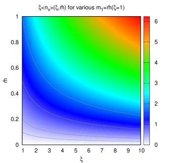
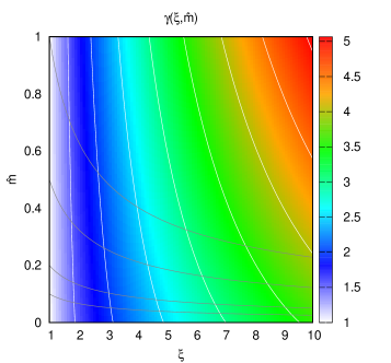
Figure 2: Anisotropy calibration at finite quark mass: Left: Lines of constant physics: fixed $m_{q}\bar{\psi}\psi$, which defines $\hat{m}(\xi)$ with $\hat{m}_{1}=\hat{m}(\xi=1)=am_{q}$. Right: bare anisotropy $\gamma$ as a function of $\xi$ and $\hat{m}$.

With the calibration results, the continuous time limit $N_{t}\rightarrow\infty$ is well defined also for finite $m_{q}$ with $m_{q}/T$ fixed. The extrapolation towards continuous time is shown in Fig. 3. The non-perturbative correction factor turns out to have a simple quark mass dependence, such that the temperature and chemical potential are uniquely specified and have a well defined continuous time limit also at finite quark mass $\hat{m}_{1}=am_{q}$:

$$\kappa(\hat{m}_{1}) =\frac{\kappa_{0}}{1+c_{1}\hat{m}_{1}+c_{2}\hat{m}_{1}^{2}} aT =\kappa(\hat{m}_{1})[aT]_{\rm mf} a\mu_{B} =\kappa(\hat{m}_{1})[a\mu_{B}]_{\rm mf}$$ (14)

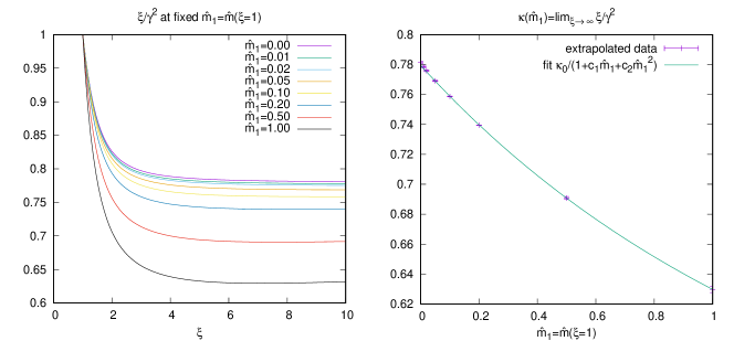
Figure 3: Example on how to obtain the continuous time limit at finite quark mass. Left: Correction factor $\xi(\gamma)/\gamma^{2}$ at fixed $\hat{m}_{1}$. Right: Dependence of the correction factor $\kappa$ in the continuous time limit on $m_{q}$.

By fixing the temperature $aT$ on a lattice specified by $N_{t}$, and the isotropic bare quark mass $\hat{m}_{1}=am_{q}$, one can determine via $\xi=aTN_{t}$ the corresponding $\hat{m}(\xi)$ and $\gamma_{0}(\xi,\hat{m}(\xi))$ for the Monte Carlo simulations. With this it is possible to measure various thermodynamic observables at fixed mass in the $\mu_{B}$-$T$ plane. Results on the phase boundary at $m_{q}>0$ have already been addressed in [17], but here the mass-independent mean field definitions $aT$ and $a\mu_{B}$ were used. The new results for the thermodynamic observables Eqs. (4)-(7), are shown in Fig. (4) for $am_{q}=0.1$.

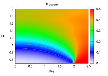
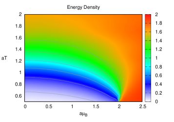
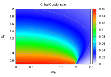
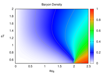
Figure 4: Various thermodynamic observables in the $\mu_{B}$ - $T$ plane at quark mass $am_{q}=0.1$. The imprint of the chiral critical endpoint at around $(aT,a\mu_{B})\simeq(0.6,2.0)$ can clearly be seen in all observables.

arrgb0.0, 0.7, 0.0

5 Conclusions

We have shown how to extend the anisotropy calibration to finite quark mass to obtain the bare anisotropy $\gamma_{0}(\xi,\hat{m}(\xi))$ given $\xi=\frac{a_{s}}{a_{t}}$ corresponds to a physically isotropic lattice: $a_{s}N_{s}=a_{t}N_{t}$. Here, the difficulty was addressed that $\gamma_{0}$ now also depends on $\hat{m}$, which requires an additional condition that keeps the physics constant and yields $\hat{m}=\hat{m}(\xi)$. This allows us to define the temperature/chemical potenital and measure thermodynamic observables such as energy and pressure unambiguously. Simulations in the continuous time limit $\xi\rightarrow\infty$ confirm the extrapolated results (see also the contribution to this conference [14]). In the future, we want to address the anisotropy calibration also for $\beta>0$: Here, the non-perturbative determination of $a_{s}/a_{t}\equiv\xi(\gamma,\hat{m},\beta)$ now also involves $\beta$, and it might be necessary to introduce an additional bare anisotropy $\beta_{s}/\beta_{t}$ as well.

6 Acknowledgment

We thank Philippe de Forcrand and Hélvio Vairinhos for useful discussions. Numerical simulations were performed on the OCuLUS cluster at PC² (Universität Paderborn). We acknowledge support by the Deutsche Forschungsgemeinschaft (DFG) through the Emmy Noether Program under Grant No. UN 370/1 and through the Grant No. CRC-TR 211 “Strong-interaction matter under extreme conditions”.

References

- [1] C. Gattringer, T. Kloiber and V. Sazonov, Nucl. Phys. B897 (2015) 732 [1502.05479].
- [2] P. Rossi and U. Wolff, Nucl. Phys. B248 (1984) 105.
- [3] F. Karsch and K. H. Mutter, Nucl. Phys. B313 (1989) 541.
- [4] P. de Forcrand and M. Fromm, Phys. Rev. Lett. 104 (2010) 112005 [0907.1915].
- [5] P. de Forcrand, J. Langelage, O. Philipsen and W. Unger, Phys. Rev. Lett. 113 (2014) 152002 [1406.4397].
- [6] G. Gagliardi, J. Kim and W. Unger, EPJ Web Conf. 175 (2018) 07047 [1710.07564].
- [7] G. Gagliardi and W. Unger, PoS LATTICE2018 (2018) 224 [1811.02817].
- [8] C. Gattringer and C. Marchis, Nucl. Phys. B916 (2017) 627 [1609.00124].
- [9] O. Borisenko, V. Chelnokov and S. Voloshyn, EPJ Web Conf. 175 (2018) 11021 [1712.03064].
- [10] N. Bilic, F. Karsch and K. Redlich, Phys. Rev. D45 (1992) 3228.
- [11] P. de Forcrand, P. Romatschke, W. Unger and H. Vairinhos, PoS LATTICE2016 (2017) 086 [1701.08324].
- [12] P. de Forcrand, W. Unger and H. Vairinhos, Phys. Rev. D97 (2018) 034512 [1710.00611].
- [13] W. Unger and P. de Forcrand, PoS LATTICE2012 (2012) 194 [1211.7322].
- [14] M. Klegrewe and W. Unger, PoS LATTICE2018 (2018) 182 [1811.01614].
- [15] S. Chandrasekharan and F.-J. Jiang, Phys. Rev. D68 (2003) 091501 [hep-lat/0309025].
- [16] L. Levkova, T. Manke and R. Mawhinney, Phys. Rev. D73 (2006) 074504 [hep-lat/0603031].
- [17] J. Kim and W. Unger, PoS LATTICE2016 (2016) 035 [1611.09120].