Comment on the article “Anisotropies in the astrophysical gravitational-wave background: The impact of black hole distributions” by A.C. Jenkins et al. [arXiv:1810.13435]

Abstract

We investigate the discrepancy pointed out by Jenkins et al. in Ref. Jenkins et al. (2018a) between the predictions of anisotropies of the astrophysical gravitational wave (GW) background, derived using different methods in Cusin et al. Cusin et al. (2018a) and in Jenkins et al. Jenkins et al. (2018b). We show that this discrepancy is not due to our treatment of galaxy clustering, contrary to the claim made in Ref. Jenkins et al. (2018a) and we show that our modeling of clustering gives results in very good agreement with observations. Furthermore we detail that the power law spectrum used in Refs. Jenkins et al. (2018a) and Jenkins et al. (2018b) to describe galaxy clustering is incorrect on large scales and leads to a different scaling for the multipoles $C_{\ell}$. Moreover, we also explain that the analytic derivation of the gravitational wave background correlation function in Refs. Jenkins et al. (2018a) and Jenkins et al. (2018b) is mathematically ill-defined and predicts an amplitude of the angular power spectrum which depends on the (arbitrary) choice of a non-physical cut-off.

Following the development of a framework to describe the anisotropies of the stochastic gravitational wave (GW) background Cusin et al. (2017, 2018b), two predictions for its amplitude in the LIGO frequency band have been proposed in the literature: the first predictions were presented in our letter Cusin et al. (2018a) followed by those of Ref. Jenkins et al. (2018b). Both studies consider the contribution of binary black hole mergers and rely on the same analytic framework designed in Ref. Cusin et al. (2017).

As explained in Refs. Cusin et al. (2017)-Cusin et al. (2018b), the expression for anisotropies has two components entering in a multiplicative way, see e.g. Eq. (72) of Ref. Cusin et al. (2017): (1) an astrophysical part which describes the process of GW emission inside a galaxy and which depends on the details of sub-galactic physics and (2) a cosmological component which describes the transfer function of cosmological perturbations, galaxy clustering and GW propagation along the line of sight. Refs. Cusin et al. (2018a) and Jenkins et al. (2018b) differ in at least two aspects: the choice of the astrophysical model and the treatment of density perturbations and galaxy clustering. For the latter, Ref. Jenkins et al. (2018b) relies both on an analytic approach and on the input from the Millennium Simulation while Ref. Cusin et al. (2018a) describes the clustering by means of a bias function while metric perturbations, velocities and matter overdensity are evolved from initial power spectra after inflation using a Bolzmann code (CMBquick CMB ) and including non linearities using Halofit Smith et al. (2003); Takahashi et al. (2012). The astrophysical models used in Refs. Jenkins et al. (2018b) and Cusin et al. (2018a) are also different. The resulting amplitude of the angular power spectrum differs between these two studies. On this basis, it was not clear whether this discrepancy is due to the different astrophysical model used in the two predictions, or to the different description of galaxy clustering.

This discrepancy was recently investigated in Ref. Jenkins et al. (2018a) by some of the authors of Ref. Jenkins et al. (2018b). They use the astrophysical model proposed in Ref. Jenkins et al. (2018b) and then derive predictions for the GW angular power spectrum both using the approach of Ref. Jenkins et al. (2018b) and the one of Ref. Cusin et al. (2018a) to describe galaxy clustering. They find a discrepancy of two orders of magnitude between these two calculations (see in particular Fig. 2 in Ref. Jenkins et al. (2018a)) and conclude that its origin lies in the description of galaxy clustering, since the astrophysical model was taken to be the same. As a consequence, they claim that the method of Ref. Cusin et al. (2018a) fails in describing galaxy clustering. We explain in the following why this conclusion is erroneous. Since in Refs. Jenkins et al. (2018b, a) (Jenkins et al. hereafter) the analytic approach to the description of clustering gives results claimed to be consistent with the ones obtained from the numerical simulation, we focus in the following on the analytic approach of Jenkins et al. We show that the power law correlation function used by Jenkins et al. does not provide a realistic description of galaxy clustering. Moreover, we show that the mathematical approach used in Jenkins et al. to compute the GW background correlation function is not correct and leads to a result which depends on the (arbitrary) choice of a nonphysical cut-off, introduced to regularize an otherwise divergent integral. Summarizing, we show in detail that the approach of Jenkins et al. used to compute the angular power spectrum of the background leads to: (1) an incorrect estimate of the shape of the angular power spectrum of the background (2) an arbitrariness in the prediction of its amplitude, since it is cut-off dependent. We also explain how to obtain consistent results, with a proper (and standard) analytic treatment of the galaxy correlation function. Sticking to our astrophysical model, we derive in a mathematically consistent way the angular power spectrum of the GW background, for both the power-law galaxy correlation function used by Jenkins et al. and for the more realistic one of Ref. Cusin et al. (2018a). In particular, our standard approach does not suffer from mathematical inconsistencies. We then address the issue of the slope of the spectrum and we show that the difference between the slope of Ref. Cusin et al. (2018a) and the one that would be obtained using the power law correlation function of Jenkins et al. is due to an overestimation of the contributions from large scales. We use the recent cosmological parameters of Ref. Ade et al. (2016) throughout.

Jenkins et al. use a power law galaxy correlation function (see Eq. (64) of Ref. Jenkins et al. (2018a))

$$\xi_{\rm Gal}(r)=\left(\frac{r}{d_{1}}\right)^{-\gamma}$$ (1)

with either a spectrum estimated from the VIMOS survey Marulli et al. (2013) with central values $d_{1}=4.29h^{-1}{\rm Mpc}$ and $\gamma=1.63$ or with parameters fitted to the numerical simulations whose central values are $d_{1}=5.05h^{-1}{\rm Mpc}$ and $\gamma=1.67$. It is claimed in Jenkins et al., and we checked it as well, that the results are nearly not affected by these differences, hence we choose the VIMOS values here. We note that the VIMOS values quoted are describing the galaxy correlation function at an average redshift of $z=0.97$. Hence in order to describe correctly the correlation function which is dominated by contributions at low redshift, it is necessary to correct it for its evolution, and as a simple estimate we consider here that the spectrum (1) needs to be multiplied by the linear growth factor

$$g^{2}\equiv\left[\frac{D_{+}(z=0)}{D_{+}(z=0.97)}\right]^{2}\simeq 1.63^{2}\simeq 2.64\,.$$ (2)

From now on, $\xi_{\rm Gal}$ refers to $g^{2}\xi_{\rm Gal}$.

The galaxy power spectrum can be inferred from the galaxy correlation function using a simple Hankel transformation Reimberg et al. (2016) as

$$P_{\rm Gal}(k)=4\pi\int\xi_{\rm Gal}(r)j_{0}(kr)r^{2}\text{d}r\,.$$ (3)

When considering the power law correlation function (1), the power spectrum is also a power law and reads

$$P_{\rm Gal}(k)=g^{2}\frac{4\pi}{k^{3}}(kd_{1})^{\gamma}\Gamma(2-\gamma)\sin(\pi\gamma/2)\,.$$ (4)

Note that from the power spectrum, the correlation function is also inferred from a Hankel transformation as

$$\xi_{\rm Gal}(r)=\int\frac{k^{2}\text{d}k}{2\pi^{2}}P_{\rm Gal}(k)j_{0}(kr)\,.$$ (5)

The galaxy correlation function and power spectrum of Jenkins et al. are plotted in dotted lines in Figs. 1 and 2.

In our approach Cusin et al. (2017), the power spectrum is obtained from the linear evolution of the nearly scale invariant power spectrum set by inflation, corrected by Halofit to account for the late-time non-linearities, and applying a scale-invariant bias $b(z)=b_{0}\sqrt{1+z}$ relating the matter fluctuations to the galaxy fluctuations. Even though we do not use the correlation function in our developments, we deduce it here for comparison using Eq. (5). Our galaxy correlation function and power spectrum are depicted in Figs. 1 and 2, in continuous line with only the linear evolution, and in dashed line with the Halofit contribution. Choosing $b_{0}=1.5$ leads to a very good agreement with the BOSS data, as can be seen by comparing the correlation function (with Halofit correction) to the Figs. 3 and 4 of Ref. Anderson et al. (2012), or the power spectrum (also with Halofit correction) to Fig. 8 of Ref. Anderson et al. (2012) (the agreement is very good with the reported bias $b(z=0.57)\simeq 1.87$).

The comparison of the spectra and correlation functions of Figs. 1 and 2 shows that the simple power law description of Jenkins et al. matches our description on the scales $2h^{-1}{\rm Mpc}\lesssim r\lesssim 20h^{-1}{\rm Mpc}$. Most notably, the power law correlation function overestimates scales larger than $20h^{-1}{\rm Mpc}$, a feature which happens to be crucial for the analytic understanding as detailed below. In the power spectrum comparison of Fig 2, it is also apparent that the power-law spectrum of Jenkins et al. fails to capture the smaller Fourier modes.

Figure 1: Correlation function used in our treatment with and without Halofit (dashed and solid line respectively) and the analytic approximation used by Jenkins et al. (dotted line).

Figure 2: Power spectrum used in our treatment with and without Halofit (dashed and solid line respectively) and the analytic approximation for the power spectrum derived from Jenkins et al. (dotted line).

We have shown in Ref. Cusin et al. (2017, 2018b) how the multipoles of the fluctuations of the GW background from astrophysical sources can be estimated. Given that the 2-point correlator of the cosmological fluctuations is diagonal in Fourier space due to statistical homogeneity, it is standard practice to derive theoretical expressions for the angular correlation function of any cosmological observable (or its corresponding $C_{\ell}$) which involve integrations on the power spectrum. In particular this allows one to obtain rigorously the plane parallel approximation (see e.g. Ref. Reimberg et al. (2016)), and the Limber approximation for extended sources (see e.g. Refs. LoVerde and Afshordi (2008); Bernardeau et al. (2011)). However instead of relying on a Limber approximation for the expression for the angular correlation function, Jenkins et al. assume that the correlation function between a point in a direction $\hat{e}_{1}$ and at redshift $z_{1}$ (that is at the associated comoving distance $r_{1}(z_{1})$ on our past line cone) and another point in direction $\hat{e}_{2}$ and at redshift $z_{2}$, is given by

$$\langle\delta_{\rm Gal}(z_{1},\hat{e}_{1})\delta_{\rm Gal}(z_{2},\hat{e}_{2})\rangle=\xi_{\rm Gal}(r_{z_{1}\hat{e}_{1},z_{2}\hat{e}_{2}})\delta(z_{1}-z_{2})\,,$$ (6)

where $r_{z_{1}\hat{e}_{1},z_{2}\hat{e}_{2}}$ is the comoving distance between these two points. This is obviously not correct since correlations at different times or different redshifts exist as cosmological fluctuations are all related by transfer functions to the initial correlations set by inflation. Equation (6) could naively seem to be a special case of a Limber approximation, but this is not the case. It is based on the wrong idea that since we observe on our past light-cone, points observed at very different redshifts are also necessarily very far apart and thus very little correlated. But this information is already contained in the correlation function $\xi_{\rm Gal}(r)$ which dies off for scales larger than the baryon acoustic oscillations scale, that is for scales larger than $150$ Mpc. A first issue arises immediately when we consider the correlation (6) for the same direction $\hat{e}_{1}=\hat{e}_{2}$, that is with no angular separation. In that case, the Dirac delta function in Eq. (6) is equivalent to changing the shape of the correlation function, causing it to vanish for finite distances. It corresponds to white noise in the redshift dependence which is unphysical. But the most serious issue is that it leads to the expression of the multipoles given by Eq. (67) of Ref. Jenkins et al. (2018b), and this is ill-defined as we shall now show.

In full generality, the monopole of the background takes the form

$$\bar{\Omega}(f)=\int_{0}^{z_{\rm max}}\text{d}z\partial_{z}\bar{\Omega}(f,z)\,,$$ (7)

meaning that any model boils down to deriving what is the contribution per unit of redshift to the total background. For instance in Refs. Cusin et al. (2017, 2018a), this is given by

$$\partial_{z}\bar{\Omega}(f,z)\equiv\frac{f}{4\pi\rho_{c}H(z)}{\cal A}(f,\eta(z))\,.$$ (8)

Using Eq. (6), it is shown in Ref. Jenkins et al. (2018b) that the multipoles of the anisotropies for the GW background take the form

$$C^{\text{Jenkins}}_{\ell}(f)=2\pi\bar{\Omega}^{2}(f){\cal A}_{\rm GW}(f)\,c_{\ell}$$ (9)

with

$$c_{\ell}\equiv\int_{-1}^{+1}\text{d}\cos\theta P_{\ell}(\cos\theta)\left[\tan(\theta/2)\right]^{-\gamma}\,,$$ (10)

$${\cal A}_{\rm GW}(f)\equiv\bar{\Omega}^{-2}(f)\int_{0}^{z_{\rm max}}\text{d}z\frac{d_{1}^{\gamma}}{[2r(z)]^{\gamma}}\left[\partial_{z}\bar{\Omega}(f,z)\right]^{2}\,.$$ (11)

We observe that for $\gamma>1$ the integrand function diverges at $z=0$, unless $\partial_{z}\bar{\Omega}(f,z=0)=0$. However, no model would predict reasonably that $\partial_{z}\bar{\Omega}(f,z)$ vanishes at $z=0$, since this would imply that there is no gravitational-wave production in our vicinity, i.e. no merging events nearby, which would be in contradiction with the LIGO BH-merger detections (with luminosity distance roughly in the range 200 to 1500 Mpc, i.e. with redshift in the range 0.05 to 0.3). Given that $z\simeq Hr$ at low redshifts, we see immediately that for $\gamma>1$, the expression (11) is not defined. The only possibility to obtain a finite result is to start the integration at a redshift $z_{\rm min}$ corresponding to a $r_{\rm min}$. But then the result obtained is completely arbitrary as it strongly depends on the cut-off. Using our astrophysical model, we infer that to obtain ${\cal A}_{\rm GW}$ of the order of $10^{-4}$ as quoted in Jenkins et al., one must use $z_{\rm min}\simeq 0.033$ corresponding to a minimum distance $r_{\rm min}\simeq 150{\rm Mpc}$, which is impossible to justify physically. In Fig. 3, we report the angular power spectrum (9) for various cut-off redshifts $z_{\rm min}$. It can be checked that they follow the scaling $c_{\ell}\propto\ell^{\gamma-2}$, hence $\ell(\ell+1)C_{\ell}/(2\pi)\propto\ell^{\gamma}$. Hence, Eq. (11) does not allow one to obtain the amplitude of the signal. Moreover, as we will show in the following, Eq. (10) provides the wrong scaling of the angular power spectrum.

In order to compute correctly the multipoles, and as for any cosmological observable, one needs to use the expressions for the angular correlations which use the power spectrum instead of the correlation function, and which are presented in Ref. Cusin et al. (2017). When considering only the dominant effect of galaxy density fluctuations, and estimating these fluctuations by their value today (hence neglecting the linear growth), the angular correlation of the gravitational waves background takes the simple form (omitting the dependence on the GW frequency $f$)

$$C(\hat{e}_{1},\hat{e}_{2})\simeq\int\text{d}r_{1}\text{d}r_{2}\partial_{r_{1}}\bar{\Omega}(r_{1})\partial_{r_{2}}\bar{\Omega}(r_{2})\xi_{\rm Gal}(r_{r_{1}\hat{e}_{1},r_{2}\hat{e}_{2}})\,,$$ (12)

where $\partial_{r}\bar{\Omega}(r)=H\partial_{z}\bar{\Omega}(z(r))$. Using the transformation (5) and Eq. (A.12) of Ref. Reimberg et al. (2016) we find the classic expression for the corresponding multipoles

$$C_{\ell}^{\text{std}}\simeq\frac{2}{\pi}\int k^{2}\text{d}kP_{\rm Gal}(k)\left|\int\partial_{r}\bar{\Omega}(r)j_{\ell}(kr)\text{d}r\right|^{2}\,.$$ (13)

We refer to this expression for the angular power spectrum as standard since it is based on the usual computational method of angular power spectra.

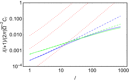
Figure 3: Angular power spectrum of relative fluctuations in the astrophysical GW background at $f=32\rm Hz{}$. Red: multipoles computed using both the power-law galaxy spectrum and analytic method of Jenkins et al. [Eq. (9) of this note] with cut-offs $z_{\rm min}=0.0033,0.033,0.33$ from top to bottom. Blue: multipoles computed using both our galaxy spectrum (CMBquick + Halofit) and our standard method to compute the angular power spectrum [essentially Eq. (13) with density growth functions properly taken into account], along with our analytic estimate of its scaling in dashed line [based on Eq. (18)]. Green: multipoles computed using the power-law spectrum of Jenkins et al. corrected by Eq. (2), but using our standard method for the angular power spectrum, along with the Limber result (19) in dashed line. In all curves we use our astrophysical model. The blue and green curves differ on large angular scales (small $\ell$) because the galaxy power spectra used in the two predictions also differ on large scales (small Fourier modes). However, only our galaxy spectrum provides an accurate description of these large scales, as shown in the text. The continuous and dashed green curve do not match for large $\ell$, even though the Limber approximation converges as $1/\ell^{2}$, because we are using a cut-off $k_{\rm max}\simeq 5\,{\rm Mpc}^{-1}$ when evaluating Eq. (13). Our result (blue curve) is much less sensitive to this cut-off because for larger modes we have less power than the power law spectrum. The blue continuous and dashed curves differ for large $\ell$ essentially because we also ignored the variations of the densities and $\partial_{r}\bar{\Omega}$ when deriving the approximation (18). The red curves are all incorrect because they are based on an ill-defined method to compute the angular power spectrum of the background, as explained in the text.

In practice, it then allows one to use the Limber approximation LoVerde and Afshordi (2008); Bernardeau et al. (2011). One method consists in noticing that for a test function $f(x)$

$$\int\text{d}xj_{\ell}(x)f(x)\simeq\sqrt{\frac{\pi}{2\ell+1}}f(\ell+1/2)\,.$$ (14)

This leads to the two equivalent formulations of the Limber approximation

$$C^{\rm Limber}_{\ell} \simeq \int\frac{\text{d}r}{r^{2}}P_{\rm Gal}(k)\left|\partial_{r}\bar{\Omega}(r)\right|^{2}\,,$$ (15)

$$C^{\rm Limber}_{\ell} \simeq \left(\ell+\tfrac{1}{2}\right)^{-1}\int\text{d}kP_{\rm Gal}(k)\left|\partial_{r}\bar{\Omega}(r)\right|^{2}\,,$$ (16)

where $k$ and $r$ must satisfy the Limber constraint

$$k\,r=\ell+\frac{1}{2}\,\,.$$ (17)

In fact, the Limber approximation can also be understood as a special case of the flat-sky approximation, and in that case a Dirac delta function enforcing equal conformal distance correlation appears naturally (see e.g. Ref. Bernardeau et al. (2011), section IIIA). This is another way to be convinced that Eq. (6) is an incorrect shortcut.

We observe that if the galaxy power spectrum has a power-law functional dependence, the Limber approximation automatically gives the slope of the background angular power spectrum. However, if the functional dependence is more complex, it is useful to introduce the further assumption that the emission is constant in redshift. More in detail, using Eq. (16) and assuming further that we can ignore the variations of $\partial_{r}\bar{\Omega}$, we then find that the multipoles are approximately given by

$$C^{\text{Limber+static}}_{\ell}\propto\frac{\left(\partial_{r}\bar{\Omega}|_{r=0}\right)^{2}}{\ell+\tfrac{1}{2}}\int_{k_{\rm min}(\ell)}P_{\rm Gal}(k)\text{d}k\,.$$ (18)

where $k_{\rm min}(\ell)$ is set by the fact that there is a maximum distance $r_{\rm max}$ at which we can find GW sources and thus a minimum Fourier mode set by the Limber constraint (17). We refer to the expression for the angular power spectrum (18) as Limber+static since it is based on the standard computation of the angular power spectrum (13), with the use of the Limber approximation and simplifying assumptions about the time evolution of sources (which properly captures the large angle slope of the spectrum).

We use in the following the Limber approximation to get an estimate of the scaling of the background angular power spectrum, for both the galaxy correlation function of Cusin et al. and Jenkins et al.

• With our galaxy power spectrum which describes correctly the large scales, and thus the small Fourier modes, the proportionality relation (18) is insensitive to $k_{\rm min}$ and one can replace it by $0$. Indeed for $k<k_{\rm eq}$ (with $k_{\rm eq}\simeq 0.01\,{\rm Mpc}^{-1}$ the Fourier mode entering the horizon at matter-radiation equivalence), $P_{\rm Gal}(k)\propto k^{\alpha}$ with $\alpha\simeq 1$. In particular we find that $C_{\ell}\propto\ell^{-1}$, and hence $\ell(\ell+1)C_{\ell}/(2\pi)\propto\ell$.

• With the power law spectrum of Jenkins et al. we have $P_{\rm Gal}(k)\propto k^{\gamma-3}$, meaning that in eq. (18) we are sensitive to low-$k$ and hence large distance contributions. Fortunately to compute the slope of the angular power spectrum in that case, it is not necessary to assume that variations $\partial_{r}\bar{\Omega}$ can be neglected, and one can rely on the Limber relation (15) to obtain

  $$C_{\ell}^{\rm Limber} \simeq \frac{g^{2}4\pi\Gamma(2-\gamma)\sin(\pi\gamma/2)}{\left(\ell+\tfrac{1}{2}\right)^{3-\gamma}}$$ (19)

  $$\times \int r\text{d}r\left(\frac{d_{1}}{r}\right)^{\gamma}|\partial_{r}\bar{\Omega}(r)|^{2}\,.$$

  This is the correct version of Eq. (9), that is of Eq. (67) in Ref. Jenkins et al. (2018b). Hence we find $C_{\ell}\propto\ell^{\gamma-3}$, that is $\ell(\ell+1)C_{\ell}/(2\pi)\propto\ell^{\gamma-1}$.

In Fig. 3 (blue and green lines) we compare the multipoles as obtained with our power spectrum to the ones obtained using the same astrophysical model, but with the power spectrum of Jenkins et al. corrected by the growth factor (2). Both these curves are obtained using the standard (correct) method to derive the angular power spectrum of the background, see Eq. (13). For our spectrum we also show in dashed blue line the approximate slope based on Eq. (18) whereas for the power law spectrum of Jenkins et al. we show in dashed green line Eq. (19). It can be checked visually that the power-law spectrum of Jenkins et al. overestimates the low $\ell$ multipoles as they benefit the most from the low $k$ Fourier modes which are incorrectly described by the power law. We note that the fact that the analytic approach of Jenkins et al., which we have shown to be inconsistent, is in agreement with their result obtained using a galaxy catalogue extracted from the Millennium simulation, is rather puzzling and calls for an explanation.

To conclude in a less technical way, while we agree that the discrepancy between the predictions of the astrophysical GW angular power spectrum of Refs. Cusin et al. (2018a) and Jenkins et al. mostly arises from the description of the clustering, we argue that the treatment of Jenkins et al. is flawed since their galaxy correlation function does not give a realistic description of large scales and furthermore their analytic treatment of the background correlation function is mathematically wrong. This emphasizes that a precise prediction of the stochastic GW angular spectrum requires both a proper astrophysical description of the BH formation and distribution but also of the cosmology and the distribution of the large scale structure. Fortunately, the latter is well-understood theoretically and under control from an observational point of view. In the above discussion we have detailed the agreement of our description Cusin et al. (2018a) with galaxy power spectra observations and the reasons why the one of Jenkins et al. is unsatisfactory. Further work should now be done on elucidating the dependence of the GW stochastic background anisotropies on astrophysical models and the possibility to constrain them.

Note added on CMBquick. Let us take the opportunity to emphasize that the code CMBquick CMB is distributed under the General Public License whose disclaimer, actually recalled in the code, states that it is without warranty of any kind […] including the implied warranties […] of fitness for a particular purpose. The entire risk as to the quality and performance of the program is with you. CMBquick is only meant as a pedagogical tool for CMB correlations computations, and more generally linear transfer functions, and as such it is provided with default parameters which are only suited for CMB computations. Furthermore it is written without any documentation about the astrophysical background computations and the conventions of normalisation. It is therefore very likely that the numerical results obtained from CMBquick in Ref. Jenkins et al. (2018a) are also not precise.

References

- Jenkins et al. (2018a) A. C. Jenkins, R. O’Shaughnessy, M. Sakellariadou, and D. Wysocki (2018a), eprint 1810.13435.
- Cusin et al. (2018a) G. Cusin, I. Dvorkin, C. Pitrou, and J.-P. Uzan, Phys. Rev. Lett. 120, 231101 (2018a), eprint 1803.03236.
- Jenkins et al. (2018b) A. C. Jenkins, M. Sakellariadou, T. Regimbau, and E. Slezak, Phys. Rev. D98, 063501 (2018b), eprint 1806.01718.
- Cusin et al. (2017) G. Cusin, C. Pitrou, and J.-P. Uzan, Phys. Rev. D96, 103019 (2017), eprint 1704.06184.
- Cusin et al. (2018b) G. Cusin, C. Pitrou, and J.-P. Uzan, Phys. Rev. D97, 123527 (2018b), eprint 1711.11345.
- (6) http://www2.iap.fr/users/pitrou/cmbquick.htm.
- Smith et al. (2003) R. E. Smith et al. (VIRGO Consortium), MNRAS 341, 1311 (2003), eprint astro-ph/0207664.
- Takahashi et al. (2012) R. Takahashi, M. Sato, T. Nishimichi, A. Taruya, and M. Oguri, Astrophys. J. 761, 152 (2012), eprint 1208.2701.
- Ade et al. (2016) P. A. R. Ade et al. (Planck), Astron. Astrophys. 594, A13 (2016), eprint 1502.01589.
- Marulli et al. (2013) F. Marulli et al., Astron. Astrophys. 557, A17 (2013), eprint 1303.2633.
- Reimberg et al. (2016) P. H. F. Reimberg, F. Bernardeau, and C. Pitrou, JCAP 1601, 048 (2016), eprint 1506.06596.
- Anderson et al. (2012) L. Anderson, E. Aubourg, S. Bailey, D. Bizyaev, M. Blanton, A. S. Bolton, J. Brinkmann, J. R. Brownstein, A. Burden, A. J. Cuesta, et al., MNRAS 427, 3435 (2012), eprint 1203.6594.
- LoVerde and Afshordi (2008) M. LoVerde and N. Afshordi, Phys. Rev. D78, 123506 (2008), eprint 0809.5112.
- Bernardeau et al. (2011) F. Bernardeau, C. Pitrou, and J.-P. Uzan, JCAP 1102, 015 (2011), eprint 1012.2652.