Iterative Classroom Teaching

Abstract

We consider the machine teaching problem in a classroom-like setting wherein the teacher has to deliver the same examples to a diverse group of students. Their diversity stems from differences in their initial internal states as well as their learning rates. We prove that a teacher with full knowledge about the learning dynamics of the students can teach a target concept to the entire classroom using $\mathcal{O}\left({\min\left\{{d,N}\right\}\log\frac{1}{\epsilon}}\right)$ examples, where $d$ is the ambient dimension of the problem, $N$ is the number of learners, and $\epsilon$ is the accuracy parameter. We show the robustness of our teaching strategy when the teacher has limited knowledge of the learners’ internal dynamics as provided by a noisy oracle. Further, we study the trade-off between the learners’ workload and the teacher’s cost in teaching the target concept. Our experiments validate our theoretical results and suggest that appropriately partitioning the classroom into homogenous groups provides a balance between these two objectives.

Introduction

Machine teaching considers the inverse problem of machine learning. Given a learning model and a target, the teacher aims to find an optimal set of training examples for the learner (?; ?). Machine teaching provides a rigorous formalism for various real-world applications such as personalized education and intelligent tutoring systems (?; ?), imitation learning (?; ?), program synthesis (?), adversarial machine learning (?), and human-in-the-loop systems (?; ?).

Individual teaching

Most of the research in this domain thus far, has focused on teaching a single student in the batch setting. Here, the teacher constructs an optimal training set (e.g., of minimum size) for a fixed learning model and a target concept and gives it to the student in a single interaction (?; ?; ?; ?). Recently, there has been interest in studying the interactive setting (?; ?; ?; ?), wherein the teacher focuses on finding an optimal sequence of examples to meet the needs of the student under consideration, which is, in fact, the natural expectation in a personalized teaching environment (?). (?) introduced the iterative machine teaching setting wherein the teacher has full knowledge of the internal state of the student at every time step using which she designs the subsequent optimal example. They show that such an “omniscient” teacher can help a single student approximately learn the target concept using $\mathcal{O}\left({\log\frac{1}{\epsilon}}\right)$ training examples (where $\epsilon$ is the accuracy parameter) as compared to $\mathcal{O}\left({\frac{1}{\epsilon}}\right)$ examples chosen randomly by the stochastic gradient descent (SGD) teacher.

Classroom teaching

In real-world classrooms, the teacher is restricted to providing the same examples to a large class of academically-diverse students. Customizing a teaching strategy for a specific student may not guarantee optimal performance of the entire class. Alternatively, teachers may constitute a partitioning of the students so as to maximize intra-group homogeneity while balancing the orchestration costs of managing parallel activities. (?) propose methods for explicitly constructing a minimal training set for teaching a class of batch learners based on a minimax teaching criterion. They also study optimal class partitioning based on prior distributions of the learners. However, they do not consider an interactive teaching setting.

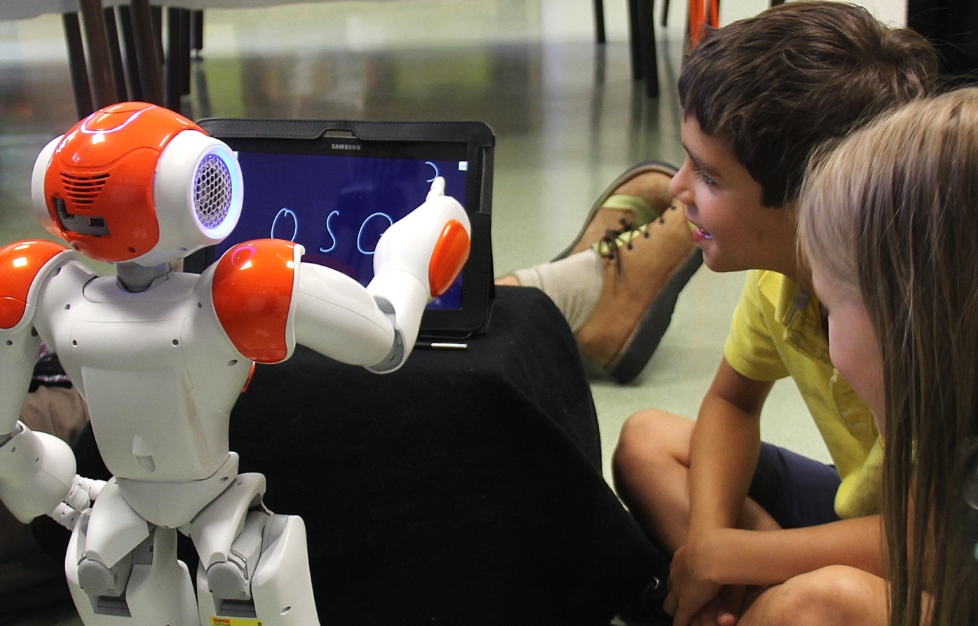
(a) A Nao robot writing on a digital tablet.

(b) Example of five interactions for writing the word ”nao”. The top row shows the writing of the robot, the bottom row shows the child’s writing.

Figure 1: The robot writes iteratively adapted to the handwriting profile of the child; if the child’s handwriting is shaky, the robot too writes with a shaky handwriting. In correcting the robot’s handwriting, the child works towards remediating theirs.

Overview of our Approach

In this paper, we study the problem of designing optimal teaching examples for a classroom of iterative learners. We refer to this new paradigm as iterative classroom teaching (CT). We focus on online projected gradient descent learners under squared loss function. The learning dynamics comprise of the learning rates and the initial states which are different for different students. At each time step, the teacher constructs the next training example based on information regarding the students’ learning dynamics. We focus on the following teaching objectives motivated by real-world classroom settings, where at the end of the teaching process:

1. all learners in the class converge to the target model (cf. Eq. (1)),

2. the class on average converges to the target model (cf. Eq. (2)).

Contributions

We first consider that setting wherein at all times, the teacher has complete knowledge of the learning rates, loss function, and full observability of the internal states of all the students in the class. A naive approach here would be to apply (?)’s omniscient teaching strategy individually for each student in the class. This would require $\mathcal{O}\left({N\log\frac{1}{\epsilon}}\right)$ teaching examples, where $N$ is the number of students in the classroom. We present a teaching strategy that can achieve a convergence rate of $\mathcal{O}\left({k\log\frac{1}{\epsilon}}\right)$, where $k$ is the rank of the subspace in which the students of the classroom lie (i.e. $k\leq\min\left\{{d,N}\right\}$, where $d$ is the ambient dimension of the problem). We also prove the robustness of our algorithm in noisy and incomplete information settings.

We then explore the idea of partitioning the classroom into smaller groups of homogenous students based on either their learning ability or prior knowledge. We also validate our theoretical results on a simulated classroom of learners and demonstrate their practical applications to the task of teaching how to classify between butterflies and moths. Further, we show the applicability of our teaching strategy to the task of teaching children how to write (cf. Figure 1).

The Model

In this section, we consider a stylized model to derive a solid understanding for the dynamics of the learners. This simplicity of our model will then allow us to gain insights into classroom partitioning (i.e., how to create classrooms), and then explore the key trade-offs between the learners’ workload as well as the teacher’s orchestration costs. By orchestration costs, we mean the number of examples the teacher needs to teach the class.

Notation

Define $\left\{{a_{i}}\right\}_{i=1}^{N}:=\left\{{a_{1},\dots,a_{N}}\right\}$ as a set of $N$ elements and $\left[{N}\right]:=\left\{{1,\dots,N}\right\}$ as the index set. For a given matrix $A$, denote $\lambda_{i}\left({A}\right)$ and $e_{i}\left({A}\right)$ to be the $i$-th largest eigenvalue of $A$ and the corresponding eigenvector respectively. $\left\|{\cdot}\right\|$ denotes the Euclidean norm unless otherwise specified. The projection operation on a set $\mathcal{W}$ for any element $y$ is defined as follows:

$$\texttt{Proj}_{\mathcal{W}}\left({y}\right)~{}:=~{} \operatorname*{arg\,min}_{x\in\mathcal{W}}\left\|{x-y}\right\|^{2}$$

Parameters

In synthesis-based teaching (?), $\mathcal{X}=\left\{{x\in\mathbb{R}^{d},\left\|{x}\right\|\leq D_{\mathcal{X}}}\right\}$ represents the feature space and the label set is given by $\mathcal{Y}=\mathbb{R}\,\text{(for regression) or }\{1,2,\ldots,m\}\,\text{(for classification)}$. A training example is denoted by $(x,y)\in\mathcal{X}\times\mathcal{Y}$. Further, we define the feasible hypothesis space by $\mathcal{W}=\left\{{w\in\mathbb{R}^{d},\left\|{w}\right\|\leq D_{\mathcal{W}}}\right\}$, and denote the target hypothesis by $w^{*}$.

Classroom

The classroom consists of $N$ students. Each student $j\in\left[{N}\right]$ has two internal parameters: i) the learning rate (at time $t$) represented by $\eta_{j}^{t}$, and ii) the initial internal state given by $w^{0}_{j}\in\mathcal{W}$. At each time step $t$, the classroom receives a labelled training example $(x^{t},y^{t})\in\mathcal{X}\times\mathcal{Y}$ and each student $j$ performs a projected gradient descent step as follows:

$$w^{t+1}_{j}~{}=~{}\texttt{Proj}_{\mathcal{W}}\left({w^{t}_{j}-\eta_{j}^{t}\frac{\partial\ell\left({\pi(w^{t}_{j},x^{t}),y^{t}}\right)}{\partial w^{t}_{j}}}\right),$$

where $\ell$ is the loss function and $\pi(w^{t}_{j},x^{t})$ is the student’s label for example $x^{t}$. We restrict our analysis to the linear regression case where $\pi(w^{t}_{j},x^{t})=\left\langle{w^{t}_{j}},{x^{t}}\right\rangle$ and $\ell\left({\left\langle{w^{t}_{j}},{x^{t}}\right\rangle,y^{t}}\right)=\frac{1}{2}\left({\left\langle{w^{t}_{j}},{x^{t}}\right\rangle-y^{t}}\right)^{2}$.

Teacher

The teacher, over a series of iterations, interacts with the students in the classroom and guides them towards the target hypothesis by choosing “helpful” training examples. The choice of the training example depends on how much information she has about the students’ learning dynamics.

• Observability: This represents the information that the teacher possesses about the internal state of each student. We study two cases: i) when the teacher knows the exact value $\left\{{w_{j}^{t}}\right\}_{j=1}^{N}$, and ii) when the teacher has a noisy estimate denoted by $\left\{{\tilde{w}_{j}^{t}}\right\}_{j=1}^{N}$ at any time $t$.

• Knowledge: This represents the information that the teacher has regarding the learning rates of each student. We consider two cases: i) when the learning rate of each student is constant and known to the teacher, and ii) when each student draws a value for the learning rate from a normal distribution at every time step, while the teacher only has access to the past values.

Teaching objective

In the abstract machine teaching setting, the objective corresponds to approximately training a predictor. Given an accuracy value $\epsilon$ as input, at time $T$ we say that a student $j\in\left[{N}\right]$ has approximately learnt the target concept $w^{*}$ when $\left\|{w^{T}_{j}-w^{*}}\right\|\leq\epsilon$. In the strict sense, the teacher’s goal may be to ensure that every student in the classroom converges to the target as quickly as possible, i.e.,

$$\left\|{w^{T}_{j}-w^{*}}\right\|~{}\leq~{}\epsilon,\,\forall{j\in\left[{N}\right]}.$$ (1)

The teacher’s goal in the average case however, is to ensure that the classroom as a whole converges to $w^{*}$ in a minimum number of interactions. More formally, the aim is to find the smallest value $T$ such that the following condition holds:

$$\frac{1}{N}\sum_{i=1}^{N}{\left\|{w_{j}^{T}-w^{*}}\right\|^{2}}~{}\leq~{}\epsilon.$$ (2)

Classroom Teaching

We study the omniscient and synthesis-based teacher, equivalent to the one considered in (?), but for the iterative classroom teaching problem under the squared loss given by $\ell\left({\left\langle{w},{x}\right\rangle,y}\right):=\frac{1}{2}\left({\left\langle{w},{x}\right\rangle-y}\right)^{2}$. Here the teacher has full knowledge of the target concept $w^{*}$, learning rates $\left\{{\eta_{j}}\right\}_{j=1}^{N}$ (assumed constant), and internal states $\left\{{w^{t}_{j}}\right\}_{j=1}^{N}$ of all the students in the classroom.

Teaching protocol

At every time step $t$, the teacher uses all the information she has to choose a training example $x^{t}\in\mathcal{X}$ and the corresponding label $y^{t}=\left\langle{w^{*}},{x^{t}}\right\rangle\in\mathcal{Y}$ (for linear regression). The idea is to pick the example which minimizes the average distance between the students’ internal states and the target hypothesis at every time step. Formally,

$$x^{t}= \operatorname*{arg\,min}_{x\in\mathcal{X}}\frac{1}{N}\sum_{j=1}^{N}{\left\|{w^{t}_{j}-\eta_{j}\frac{\partial\ell\left({\left\langle{w^{t}_{j}},{x}\right\rangle,\left\langle{w^{*}},{x}\right\rangle}\right)}{\partial w^{t}_{j}}-w^{*}}\right\|^{2}}.$$

Note that constructing the optimal example at time $t$, is in general a non-convex optimization problem. For the squared loss function, we present a closed-form solution below.

Algorithm 1 CT: Classroom teaching algorithm

  Input: target $w^{*}\in\mathcal{W}$; students’ learning rates $\left\{{\eta_{j}}\right\}_{j=1}^{N}$

  Goal: accuracy $\epsilon$

  Initialize $t=0$

  Observe $\left\{{w_{j}^{0}}\right\}_{j=1}^{N}$

  while $\frac{1}{N}\sum_{j=1}^{N}{\left\|{w_{j}^{t}-w^{*}}\right\|^{2}}>\epsilon$ do

     Observe $\left\{{w_{j}^{t}}\right\}_{j=1}^{N}$

     Choose $\gamma_{t}$ s.t. $\gamma_{t}\leq D_{\mathcal{X}}$, and $2-\eta_{j}\gamma_{t}^{2}\geq 0,\forall{j\in\left[{N}\right]}$

     Construct $W^{t}$ given by Eq. (6)

     Pick example $x^{t}=\gamma_{t}\cdot e_{1}\left({W^{t}}\right)$ and $y^{t}=\left\langle{w^{*}},{x^{t}}\right\rangle$

     Provide the labeled example $\left({x^{t},y^{t}}\right)$ to the classroom

     Students’ update: $\forall{j\in\left[{N}\right]}$,

$$w_{j}^{t+1}\leftarrow\texttt{Proj}_{\mathcal{W}}\left({w_{j}^{t}-\eta_{j}\left({\left\langle{w_{j}^{t}},{x^{t}}\right\rangle-y^{t}}\right)x^{t}}\right).$$

     $t\leftarrow t+1$

  end while

Example construction

Define, $\hat{w}_{j}^{t}~{}:=~{}{w_{j}^{t}-w^{*}}$, for $j\in\left[{N}\right]$. Then the teacher constructs the common example for the whole classroom at time $t$ as follows:

1. the feature vector $x^{t}=\gamma_{t}\hat{x}^{t}$ such that

   1. the magnitude $\gamma_{t}$:

      $$\gamma_{t}\leq D_{\mathcal{X}},\text{ and }2-\eta_{j}\gamma_{t}^{2}~{}\geq~{}0,\forall{j\in\left[{N}\right]}.$$ (3)

   2. the direction $\hat{x}^{t}$ (with $\left\|{\hat{x}^{t}}\right\|=1$):

      $$\hat{x}^{t}~{}:=~{}\operatorname*{arg\,max}_{x:\left\|{x}\right\|=1}x^{\top}W^{t}x~{}=~{}e_{1}\left({W^{t}}\right),$$ (4)

      where

      $$\alpha_{j}^{t}~{}:=~{} \eta_{j}\gamma_{t}^{2}\left({2-\eta_{j}\gamma_{t}^{2}}\right)$$ (5)

      $$W^{t}~{}:=~{} \frac{1}{N}\sum_{j=1}^{N}\alpha_{j}^{t}\hat{w}_{j}^{t}\left({\hat{w}_{j}^{t}}\right)^{\top}.$$ (6)

2. the label $y^{t}=\left\langle{w^{*}},{x^{t}}\right\rangle$.

Algorithm 1 puts together our omniscient classroom teaching strategy. Theorem 1 provides the number of examples required to teach the target concept.

Theorem 1.

Consider the teaching strategy given in Algorithm 1. Let $k:=\max_{t}\left\{{\mathrm{rank}\left({W^{t}}\right)}\right\}$, where $W^{t}$ is given by Eq. (6). Define $\alpha_{j}:=\min_{t}\alpha_{j}^{t}$, $\alpha_{\mathrm{min}}:=\min_{t,j}\alpha_{j}^{t}$, and $\alpha_{\mathrm{max}}:=\max_{t,j}\alpha_{j}^{t}$, where $\alpha_{j}^{t}$ is given by Eq. (5). Then after $t=\mathcal{O}\left({\left({\log\frac{1}{1-\frac{\alpha_{\mathrm{min}}}{k}}}\right)^{-1}\log\frac{1}{\epsilon}}\right)$ rounds, we have $\frac{1}{N}\sum_{j=1}^{N}{\left\|{w_{j}^{t}-w^{*}}\right\|^{2}}\leq\epsilon$. Furthermore, after $t=\mathcal{O}\left({\max\left\{{\left({\log\frac{1}{1-\alpha_{j}}}\right)^{-1}\log{\frac{1}{\epsilon}},\left({\log\frac{1}{1-\frac{\alpha_{\mathrm{min}}}{k}}}\right)^{-1}\log{\frac{1}{\epsilon}}}\right\}}\right)$ rounds, we have $\left\|{w_{j}^{t}-w^{*}}\right\|^{2}\leq\epsilon,\forall{j\in\left[{N}\right]}$.

Remark 1.

By using the fact that $\exp\left({-2x}\right)\leq\log\left({1-x}\right)$, for $2x\leq 1.59$, we can show that for $k\geq\frac{2\alpha_{\mathrm{min}}}{1.59}$, $\mathcal{O}\left({\left({\log\frac{1}{1-\frac{\alpha_{\mathrm{min}}}{k}}}\right)^{-1}\log\frac{1}{\epsilon}}\right)\approx\mathcal{O}\left({\frac{k}{\alpha_{\mathrm{min}}}\log\frac{1}{\epsilon}}\right)$.

Based on Theorem 1 and Remark 1, note that the teaching strategy given in Algorithm 1 converges in $\mathcal{O}\left({k\log\frac{1}{\epsilon}}\right)$ samples, where $k=\max_{t}\left\{{\mathrm{rank}\left({W^{t}}\right)}\right\}\leq\min\left\{{d,N}\right\}$. This is in fact a significant improvement (especially when $N\gg d$) over the sample complexity $\mathcal{O}\left({N\log\frac{1}{\epsilon}}\right)$ of a teaching strategy which constructs personalized training examples for each student in the classroom.

Choice of magnitude $\gamma_{t}$

We consider the following two choices of $\gamma_{t}$:

1. static $\gamma_{t}=\min\left\{{\frac{1}{\max_{j\in\left[{N}\right]}\sqrt{\eta_{j}}},D_{\mathcal{X}}}\right\}$: This ensures that the classroom can converge without being partitioned into small groups of students. However, the value $\alpha_{\mathrm{min}}$ becomes small and as a result, the sample complexity increases.

2. dynamic $\gamma_{t}=\min\left\{{\sqrt{\frac{\sum_{j=1}^{N}{\eta_{j}\left\|{w_{j}^{t}-w^{*}}\right\|^{2}}}{\sum_{j=1}^{N}{\eta_{j}^{2}\left\|{w_{j}^{t}-w^{*}}\right\|^{2}}}},D_{\mathcal{X}}}\right\}$: This provides an optimal constant for the sample complexity, but requires that for effective teaching the classroom is partitioned appropriately. This value of $\gamma_{t}$ is obtained by maximizing the term $\sum_{j=1}^{N}{\eta_{j}\gamma_{t}^{2}\left({2-\eta_{j}\gamma_{t}^{2}}\right)\left\|{w_{j}^{t}-w^{*}}\right\|^{2}}$.

Natural partitioning based on learning rates

In order to satisfy the requirements given in Eq. (3), for every student $j\in\left[{N}\right]$, we require (for dynamic $\gamma_{t}$):

$$\eta_{j}\gamma_{t}^{2}~{}\leq~{} \eta_{\text{max}}\frac{\sum_{j=1}^{N}{\eta_{j}\left\|{w_{j}^{t}-w^{*}}\right\|^{2}}}{\sum_{j=1}^{N}{\eta_{j}^{2}\left\|{w_{j}^{t}-w^{*}}\right\|^{2}}}$$

$$~{}\leq~{} \eta_{\text{max}}\frac{\sum_{j=1}^{N}{\eta_{j}\left\|{w_{j}^{t}-w^{*}}\right\|^{2}}}{\eta_{\text{min}}\sum_{j=1}^{N}{\eta_{j}\left\|{w_{j}^{t}-w^{*}}\right\|^{2}}}~{}\leq~{}2,$$ (7)

where $\eta_{\text{max}}=\max_{j}\eta_{j}$, and $\eta_{\text{min}}=\min_{j}\eta_{j}$. That is, if $\eta_{\text{max}}\leq 2\eta_{\text{min}}$, we can safely use the above optimal $\gamma_{t}$. This observation also suggests a natural partitioning of the classroom: $\left\{{[\eta_{\text{min}},2\eta_{\text{min}}),[2\eta_{\text{min}},4\eta_{\text{min}}),\dots,[2^{m}\eta_{\text{min}},2\eta_{\text{max}})}\right\}$, where $m=\left\lfloor\log_{2}\frac{\eta_{\text{max}}}{\eta_{\text{min}}}\right\rfloor$.

Robust Classroom Teaching

In this section, we study the robustness of our teaching strategy in cases when the teacher can access the current state of the classroom only through a noisy oracle, or when the learning rates of the students vary with time.

Noise in $w_{j}^{t}$’s

Here, we consider the setting where the teacher cannot directly observe the students’ internal states $\left\{{w^{t}_{j}}\right\}_{j=1}^{N},\forall t$ but has full knowledge of students’ learning rates $\left\{{\eta_{j}}\right\}_{j=1}^{N}$. Define $\alpha_{\mathrm{min}}:=\min_{t,j}\alpha_{j}^{t}$, and $\alpha_{\mathrm{avg}}:=\max_{t}{\frac{1}{N}\sum_{j=1}^{N}{\alpha_{j}^{t}}}$, where $\alpha_{j}^{t}$ is given by Eq. (5). At every time step $t$, the teacher only observes a noisy estimate of $w_{j}^{t}$ (for each $j\in\left[{N}\right]$) given by

$$\tilde{w}_{j}^{t}~{}:=~{}w_{j}^{t}+\delta_{j}^{t},$$ (8)

where $\delta_{j}^{t}$ is a random noise vector such that $\left\|{\delta_{j}^{t}}\right\|\leq\frac{\epsilon}{4\left({\frac{\alpha_{\mathrm{avg}}}{\alpha_{\mathrm{min}}}d+1}\right)D_{\mathcal{W}}}$. Then the teacher constructs the example as follows:

$$\hat{x}^{t}~{}:=~{} \operatorname*{arg\,max}_{x:\left\|{x}\right\|=1}x^{\top}\left\{{\frac{1}{N}\sum_{j=1}^{N}{\alpha_{j}^{t}{\hat{w}_{j}^{t}}\left({\hat{w}_{j}^{t}}\right)^{\top}}}\right\}x$$

$$x^{t}~{}:=~{} \gamma_{t}\hat{x}^{t}\text{ and }y^{t}=\left\langle{w^{*}},{x^{t}}\right\rangle,$$ (9)

where $\hat{w}^{t}_{j}:={\tilde{w}^{t}_{j}-w^{*}}$, and $\gamma_{t}$ satisfies the condition given in Eq. (3). The following theorem shows that even under this noisy observation setting Eq. (8), with the example construction strategy described in Eq. (9), the teacher can teach the classroom with linear convergence.

Theorem 2.

Consider the noisy observation setting given by Eq. (8). Let $k:=\max_{t}\left\{{\mathrm{rank}\left({W^{t}}\right)}\right\}$ where $W^{t}=\frac{1}{N}\sum_{j=1}^{N}{\alpha_{j}^{t}\left({\tilde{w}^{t}_{j}-w^{*}}\right)\left({\tilde{w}^{t}_{j}-w^{*}}\right)^{\top}}$. Then for the robust teaching strategy given by Eq. (9), after $t=\mathcal{O}\left({\left({\log\frac{1}{1-\frac{\alpha_{\mathrm{min}}}{k}}}\right)^{-1}\log\frac{1}{\epsilon}}\right)$ rounds, we have $\frac{1}{N}\sum_{j=1}^{N}{\left\|{w_{j}^{t}-w^{*}}\right\|^{2}}\leq\epsilon$.

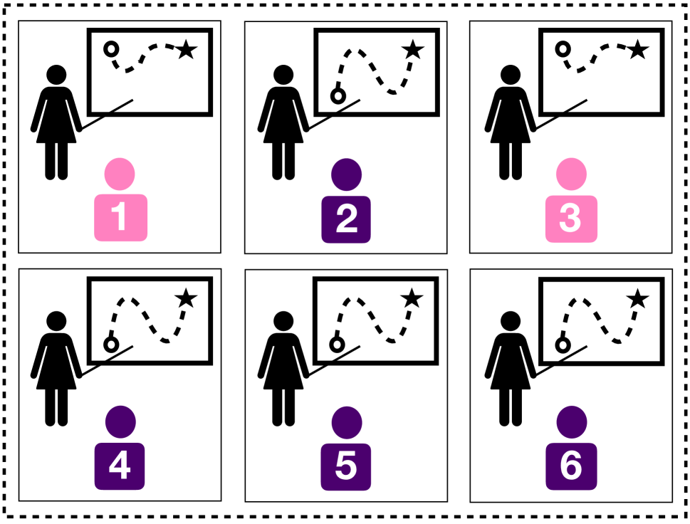
(a) Individual teaching (IT)

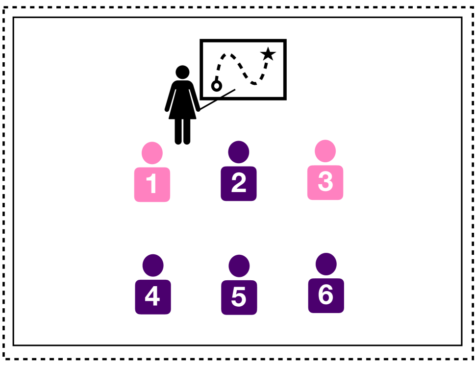
(b) Classroom teaching (CT)

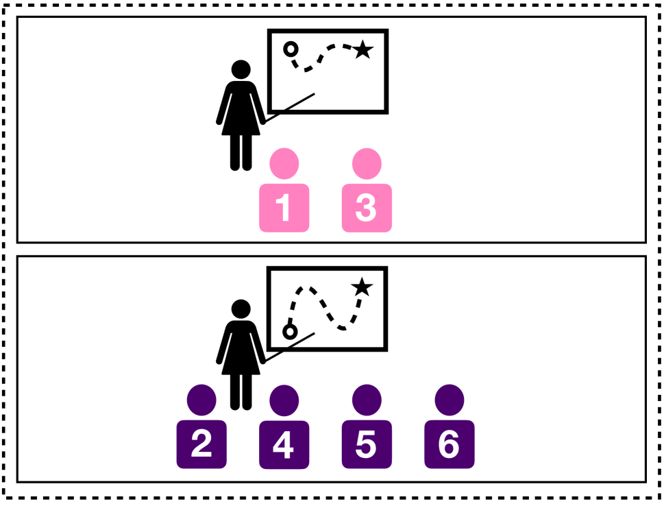
(c) Classroom teaching with partitions (CTwP)

Figure 2: Comparisons between individual teaching (IT) and classroom teaching (CT and CTwP) paradigms.

Noise in $\eta_{j}^{t}$

Here, we consider a classroom of online projected gradient descent learners with learning rates $\left\{{\eta_{j}^{t}}\right\}_{j=1}^{N}$, where $\eta_{j}^{t}\sim\mathcal{N}\left({\eta_{j},\sigma}\right)$. We assume that the teacher knows $\sigma$ (which is constant across all the students) and $\left\{{\eta_{j}}\right\}_{j=1}^{N}$, but doesn’t know $\left\{{\eta^{t}_{j}}\right\}_{j=1}^{N}$. Further, we assume that the teacher has full observability of $\left\{{w_{j}^{t}}\right\}_{j=1}^{N}$. At time $t$, the teacher has access to the history $H_{t}:=\left({\left\{{w_{j}^{s}}\right\}_{s=1}^{t},\left\{{\eta_{j}^{s}}\right\}_{s=1}^{t-1}:\forall{j\in\left[{N}\right]}}\right)$. Then the teacher constructs the example as follows (depending only on $H_{t}$):

$$\hat{x}^{t}~{}:=~{} \operatorname*{arg\,max}_{x:\left\|{x}\right\|=1}x^{\top}\bar{W}^{t}x~{}=~{}e_{1}\left({\bar{W}^{t}}\right)$$

$$x^{t}~{}:=~{} \gamma_{t}\hat{x}^{t}\text{ and }y^{t}=\left\langle{w^{*}},{x^{t}}\right\rangle,$$ (10)

where

$$\gamma_{t}^{2}~{}\leq~{} \frac{2\eta_{j}}{\sigma^{2}+\eta_{j}^{2}},\forall{j\in\left[{N}\right]}$$ (11)

$$\bar{\eta}_{j}^{t}~{}:=~{} \frac{1}{t-1}\sum_{s=1}^{t-1}{\eta_{j}^{s}}$$ (12)

$$\bar{\alpha}_{j}^{t}~{}:=~{} 2\gamma_{t}^{2}\bar{\eta}_{j}^{t}-\gamma_{t}^{4}\left({\frac{t-2}{t-1}\sigma^{2}+\left({\bar{\eta}_{j}^{t}}\right)^{2}}\right)$$ (13)

$$\hat{w}_{j}^{t}~{}:=~{} {w^{t}_{j}-w^{*}}\text{ and }$$ (14)

$$\bar{W}^{t}~{}:=~{} \frac{1}{N}\sum_{j=1}^{N}\bar{\alpha}_{j}^{t}\hat{w}_{j}^{t}\left({\hat{w}_{j}^{t}}\right)^{\top}.$$ (15)

The following theorem shows that, in this setting, the teacher can teach the classroom in expectation with linear convergence.

Theorem 3.

Let $k:=\max_{t}\left\{{\mathrm{rank}\left({\bar{W}^{t}}\right)}\right\}$ where $\bar{W}^{t}$ is given by Eq. (15). Define $\bar{\alpha}_{\mathrm{min}}:=\min_{t,j}\bar{\alpha}_{j}^{t}$, and $\beta_{\mathrm{min}}:=\min_{j,t}{\frac{\alpha_{j}^{t}}{\bar{\alpha}_{j}^{t}}}$, where $\alpha_{j}^{t}:=2\gamma_{t}^{2}\eta_{j}-\gamma_{t}^{4}\left({\sigma^{2}+\eta_{j}^{2}}\right)$ and $\bar{\alpha}_{j}^{t}$ given by Eq. (13). Then for the teaching strategy given by Eq. (10), after $t=\mathcal{O}\left({\left({\log\frac{1}{1-\frac{\beta_{\mathrm{min}}\bar{\alpha}_{\mathrm{min}}}{k}}}\right)^{-1}\log\frac{1}{\epsilon}}\right)$ rounds, we have $\mathbb{E}\left[{\frac{1}{N}\sum_{j=1}^{N}{\left\|{w_{j}^{t}-w^{*}}\right\|^{2}}}\right]\leq\epsilon$.

Classroom Partitioning

Individual teaching can be very expensive due to the effort required in producing personalized education resources. At the same time, classroom teaching increases the students’ workload substantially because it requires catering to the needs of academically diverse learners. We overcome these pitfalls by partitioning the given classroom of $N$ students into $K$ groups such that the orchestration cost of the teacher and the workload of students is balanced. Figure 2 illustrates these three different teaching paradigms.

Let $T(K)$ be the total number of examples required by the teacher to teach all the groups. Let $S(K)$ be the average number of examples needed by a student to converge to the target. We study the total cost defined as:

$$\mathrm{cost}(K)~{}:=~{}T(K)+\lambda\cdot S(K),$$

where $\lambda$ quantifies the trade-off factor, and its value is application dependent. In particular, for any given $\lambda$, we are interested in that value $K$ that minimizes $\mathrm{cost}(K)$. For example, when $\lambda=\infty$, the focus is on the student workload; thus the optimal teaching strategy is individual teaching, i.e., $K=N$. Likewise, when $\lambda=0$, the focus is on the orchestration cost; thus the optimal teaching strategy is classroom teaching without partitioning, i.e., $K=1$. In this paper, we explore two homogeneous partitioning strategies: (a) based on learning rates of the students $\left\{{\eta_{j}}\right\}_{j=1}^{N}$, (b) based on prior knowledge of the students $\left\{{w_{j}^{0}}\right\}_{j=1}^{N}$.

Experiments

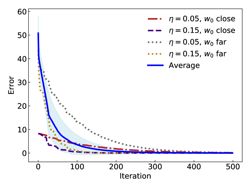
(a) Error plot for CT; average error of the classroom and the error of four selected learners.

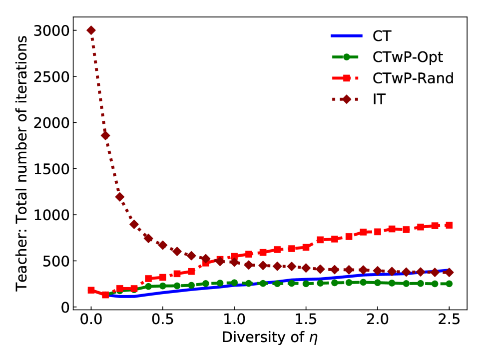
(b) Total iterations needed for convergence from the teacher’s perspective.

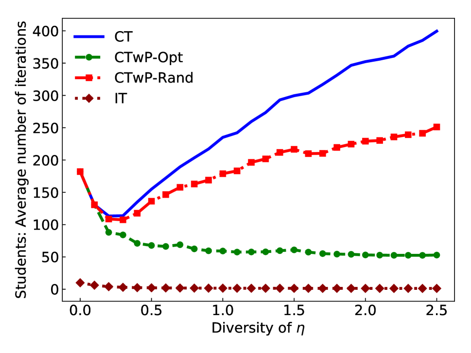
(c) Total iterations per student needed for convergence from the students’ perspective.

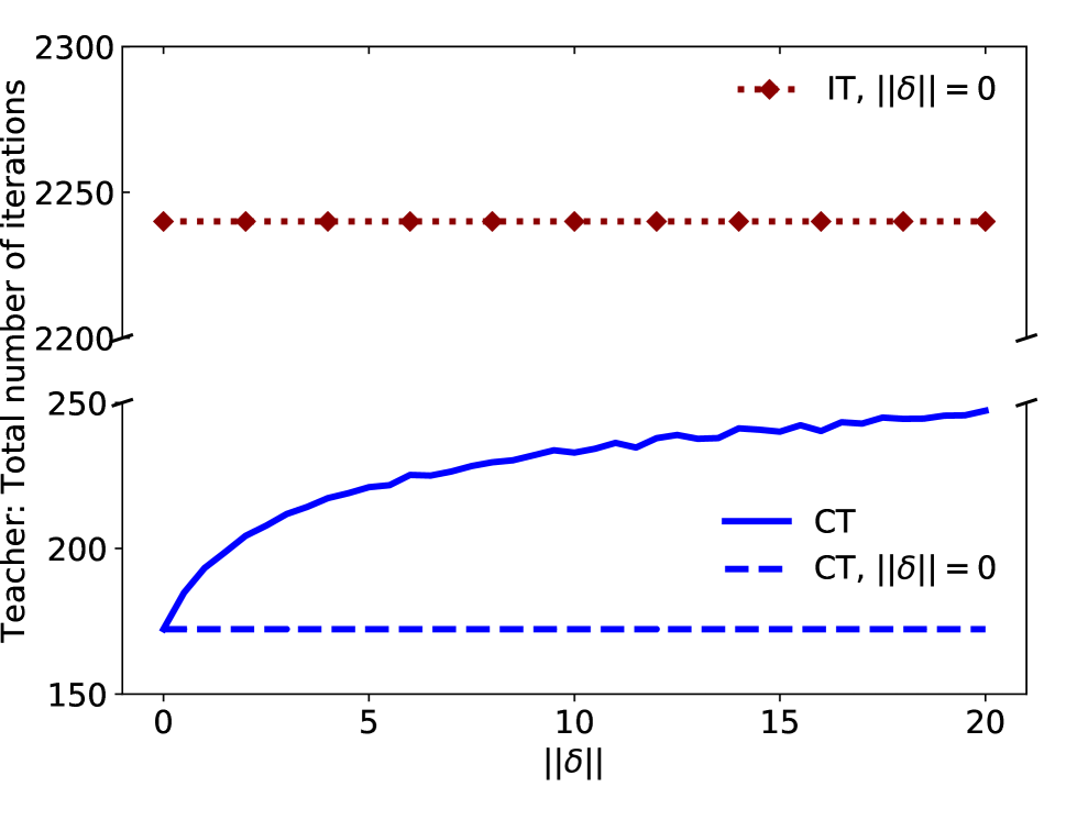
(d) Total iterations needed for convergence in noisy $w_{t}$ case as the noise, $\delta$, increases.

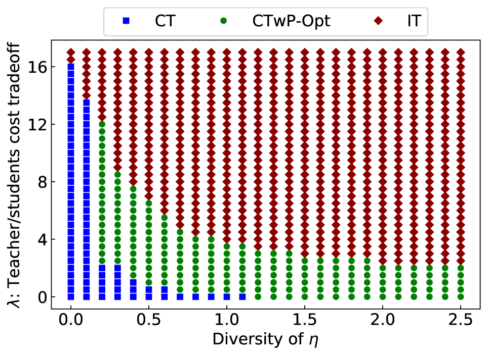
(e) $\lambda$: Trade-off between teacher’s and students’ cost with increasing $\eta$ diversity.

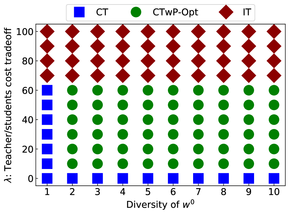
(f) $\lambda$: Trade-off between teacher’s and students’ cost with increasing $w^{0}$ diversity.

Figure 3: (3(a)) and (3(d)) show the convergence results for the noise-free and noisy settings. CT is robust and exhibits linear convergence. (3(b)), (3(c)) and (3(e)) show the convergence results and trade-off for a classroom with diverse $\eta$. (3(f)) shows the trade-off for a classroom with diverse $w^{0}$.

Teaching Linear Models with Synthetic Data

We first examine the performance of our teaching algorithms on simulated learners.

Setup  We evaluate the following algorithms: (i) classroom teaching (CT) - the teacher gives an example to the entire class at each iteration, (ii) CT with optimal partitioning (CTwP-Opt) - the class is partitioned as defined in Section Classroom Partitioning, (iii) CT with random partitioning (CTwP-Rand) - the class is randomly assigned to groups, and (iv) individual teaching (IT) - the teacher gives a tailored example to each student. An algorithm is said to converge when $\frac{1}{N}\sum_{i}\lVert w_{i}^{t}-w^{*}\rVert_{2}^{2}\leq\epsilon$. We set the number of learners $N=300$ and accuracy parameter $\epsilon=0.1$.

Average error and robustness of CT  We first consider the noise free classroom setting with $d=25$, learning rates between $[0.05,0.25]$, and $D_{\mathcal{X}}=2$. The plot of the error over time is shown in Figure 3(a), together with the performance of four selected learners. Our algorithm exhibits linear convergence, as per Theorem 1. The slower the learners and the further away they are from $w^{*}$, the longer they take to converge. Figure 3(d) shows how convergence is affected as the noise level, $\delta$, increases in the robust classroom teaching setting as described in Section Robust Classroom Teaching. Although the number of iterations required for convergence increases, it is still significantly lower than the noise-free IT.

Convergence for classroom with diverse $\eta$  We study the effect of partitioning by $\eta$ on the performance of the algorithms described. The diversity of the classroom varies from 0 (where all learners in the classroom have $\eta=0.1$) to 0.5 (where for all learners $\eta\in[0.1,0.6]$ chosen randomly), and so on. Figure 3(b) and Figure 3(c) depict the number of iterations and number of examples needed by the teacher and students respectively to achieve convergence. As expected, IT performs best, and CTwP-Opt consistently outperforms CT. For a class with low diversity, partitioning is costly. However as diversity increases, partitioning is beneficial from the teachers’ perspective. Note that the dip at a diversity of 0.15 for both plots is due to the value of $D_{\mathcal{X}}$. For the static $\gamma_{t}$, with $D_{\mathcal{X}}=2$, all learners with rates less than 0.25 will be negatively affected. As the minimum value of $\eta$ is 0.1, at zero diversity, all learners are affected the most. As diversity increases to 0.15, all learners are affected but to a lesser degree. Figure 3(e) shows how the optimal algorithm, the one that minimizes cost, changes with $\lambda$ and diversity of $\eta$. When diversity is low and there is a low trade-off factor on the students’ workload, CT performs best. At high values, IT has the lowest cost. CTwP-Opt falls between these two regimes.

Convergence for classroom with diverse $w^{0}$  Next, we study partitioning based on prior knowledge. We generate each cluster from a Gaussian distribution centered on a point along different axes. At diversity 1, all 300 learners are centered on a point on one axis, whereas at diversity 2, 150 learners are centered on one axis and the other 150 on another. Thus at 10, we have 30 learners around a point at each of the 10 axes. Each cluster represents one partition. Although the convergence plots from the teacher and students’ perspective are not presented, they exhibit the same behaviour as partitioning by $\eta$. Figure 3(f) shows the cost trade off plot in 10 dimensions as the number of clusters of $w^{0}$ increase. The results are the same as with $\eta$ partitioning and CTwP-Opt outperforms in most regimes.

Teaching How to Classify Butterflies and Moths

We now demonstrate the performance of our teaching algorithms on a binary image classification task for identifying insect species, a prototypical task in crowdsourcing applications and an important component in citizen science projects such as eBird (?).

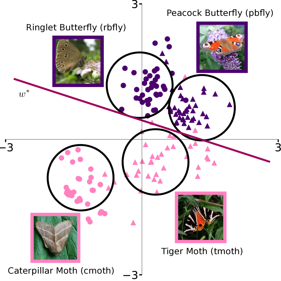
(a) Dataset of images $\mathcal{X}$ and target $w^{*}$

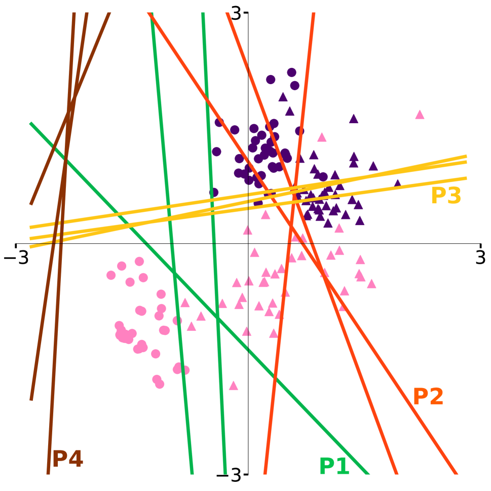
(b) Initial $w^{0}$ of 4 types of learners

(c) Teaching examples, visualized twice every 10 iterations.

(d) Total iterations needed for convergence from the teacher’s perspective

(e) Total iterations needed for convergence from the student’s perspective

(f) $\lambda$: Trade-off between teacher’s and students’ cost with increasing $w_{0}$ diversity

Figure 4: (4(a)) shows a low-dimensional embedding of the dataset and the target concept. (4(b)) shows an embedding of the initial states of three learners of each of the 4 types. (4(c)) are training examples selected by CT and CTwP-Opt teachers when the class has diversity 4. (4(d)) and (4(e)) show the number of iterations required to achieve $\epsilon$-convergence from the teacher and student perspectives. (4(f)) shows how the optimal algorithm changes as we vary the trade-off parameter $\lambda$, and diversity of the class.

Images and Euclidean embedding  We use a collection of 160 images (40 each) of four species of insects, namely (a) Caterpillar Moth (cmoth), (b) Tiger Moth (tmoth), (c) Ringlet Butterfly (rbfly), and (d) Peacock Butterfly (pbfly), to form the teaching set $\mathcal{X}$. Given an image, the task is to classify if it is a butterfly or a moth. However, we need a Euclidean embedding of these images so that they can be used by a teaching algorithm. Based on the data collected by (?), we obtained binary labels (whether a given image is a butterfly or not) for $\mathcal{X}$ from a set of 67 workers from Amazon Mechanical Turk. Using this annotation data, the Bayesian inference algorithm of (?) allows us to obtain an embedding, shown in Figure 4(a), along with the target $w^{*}$ (the best fitted linear hypothesis for $\mathcal{X}$).

Learners’ hypotheses  The process described above to obtain the embedding in Figure 4(a) simultaneously generates an embedding of each of the $67$ annotators as linear hypotheses in the same 2D space. Termed as “schools of thought” by (?), these hypotheses capture various real-world idiosyncrasies in the AMT workers’ annotation behavior. For our experiments, we identified four types of learners’ hypotheses; those who (i) misclassify tmoth as butterfly (P1), (ii) misclassify rbfly as moth (P2), (iii) misclassify pbfly as moth (P3) and (iv) misclassify tmoth and cmoth as butterflies. Figure 4(b) shows an embedding of three distinct hypotheses each of the four types of learners.

Creating the classroom  We denote the hypotheses described above as initial states $w^{0}$ of the learners/students. Due to sparsity of data, we create a supersample of size $60$ for the four types of learners by adding a small noise. We set the classroom size $N=60$. The diversity of the class, defined by the number of different types of learners present, varies from 1 to 4. Thus, diversity of $1$ refers to the case when all $60$ learners are of same type (randomly picked from P1, P2, P3, or P4), and diversity of $4$ refers to the case when there are $15$ learners of each type. We set a constant learning rate of $\eta=0.05$ for all students.

Teaching and performance metrics  We study the performance of CT, CTwP-Rand, and IT teachers. We also examine the CTwP-Opt teacher that partitions the learners of the class based on their types. All teachers are assumed to have complete information about the learners at all times. We set accuracy parameter $\epsilon=0.2$ and the classroom is said to have converged when $\frac{1}{N}\sum_{i}\lVert w_{i}^{t}-w^{*}\rVert_{2}^{2}\leq\epsilon$.

Teaching examples  Figure 4(c) consists of 5 rows of 20 thumbnail images each, depicting the training examples chosen in an actual run of the experiment when the diversity of the classroom is 4. The first row corresponds to the images chosen by CT. For instance, in iteration 1, CT chooses a tmoth example. While this example is most helpful for learners in P1 (confusing tmoths as butterflies), however, learners in P2 and P3 would have benefited more from seeing examples of butterflies. This increases the workload for the learners. The next four rows in Figure 4(c) correspond to the images chosen by CTwP-Opt when teaching partitions P1, P2, P3, and P4 respectively—these thumbnails show the personalized effect given the homogeneity of these partitions. For instance, for P1, the CTwP-Opt focuses on choosing tmoth examples thereby allowing these learners to converge faster while ensuring that the cost for learners in other partitions does not increase.

Convergence  Figure 4(d) compares the performances of the teachers in terms of the total number of iterations required for convergence. CT performs optimally because every example chosen is provided to the entire class; CTwP-Opt requires only a few examples more, given the homogeneity of the partition and the partitions being of equal size. IT constructs individually tailored examples for each learner in the class. Thus the combined number of iterations is much higher in comparison.

Teacher/students cost trade-off  On the other hand, Figure 4(e) depicts the average number of examples required by each learner to achieve convergence as a function of diversity. This represents the learning cost from the students’ persective. IT performs best because the teacher chooses personalized examples for each learner. CTwP-Opt performs considerably better than CT. This happens because partitioning groups together learners of the same type. Figure 4(f) represents optimal algorithm given the diversity of the class and the trade-off factor $\lambda$ as defined in Section Classroom Partitioning. As diversity increases, CTwP-Opt outperforms the other teachers in terms of the total cost.

(a) Shaky and distorted handwriting

(b) Shaky and rotated handwriting

(c) Rotated and distorted handwriting

Figure 5: (5(a)) to (5(c)) shows samples of children’s handwriting where two of the three defined features are poor and the third is good.

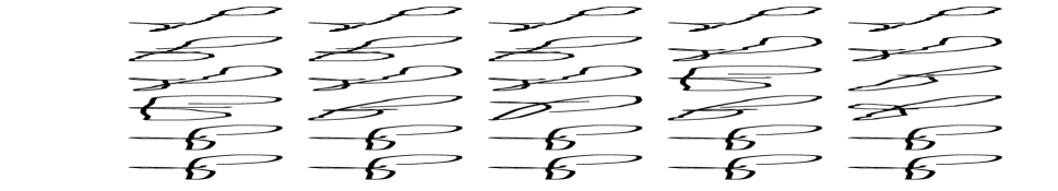
(a) Teaching examples for shaky and rotated handwriting

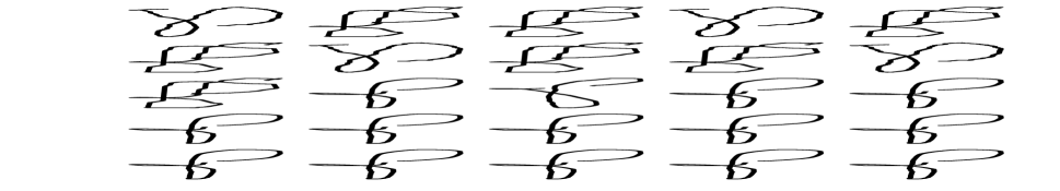
(b) Teaching examples for distorted and shaky handwriting

(c) Teaching examples for distorted and rotated handwriting

(d) Teaching examples for distorted, rotated, shaky handwriting

Figure 6: (6(a)) to (6(d)) shows the sequence of examples, visualized every other iteration, chosen by our algorithm for different initial hypothesis of the children.

Teaching How to Write

Despite formal training, between 5% to 25% of children struggle to acquire handwriting skills. Being unable to write legibly and rapidly limits a child’s ability to simultaneously handle other tasks such as grammar and composition which may lead to general learning difficulties (?; ?). (?) and (?) adopt an approach where the child plays the role of the “teacher” and an agent a “learner” that needs help. This method of learning by teaching boosts a child’s self esteem and increases their commitment to the task as they are given the role of the one who “knows and teaches” (?; ?). In our experiments, a robot iteratively proposes a handwriting adapted to the handwriting profile of the child, that they try to correct (cf. Figure 1(b)). We now demonstrate the performance of our algorithm in choosing this sequence of examples.

Generating handwriting dynamics  A LSTM is used to learn and generate handwriting dynamics (?). It is trained on children’s handwriting data collected from 1014 children from 14 schools. In the Appendix, we showed that the pool of samples has to be rich enough for teaching to be effective. As our generative model outputs a distribution, we can sample from it to get a diverse set of teaching examples. We analyze our results for a cursive “f”, similar results apply for the other letters.

Handwriting features  Concise Evaluation Scale (BHK) (?) is a standard handwriting test used in Europe to evaluate children’s handwriting quality. We adopt features such as (i) distortion, (ii) rotation, (iii) shakiness, and label each generated sample with a score for each of these features.

Creating the classroom  Given a child’s handwriting sample, we estimate their initial hypothesis, $w_{0}$ by how well each of the above features have been written, in a similar fashion to the scoring of samples. As most children fair poorly in two out of the three features, we selected and partitioned them according to the following three types of handwriting characteristics, substantial (i) shakiness and rotation, (ii) distortion and shakiness, and (iii) distortion and rotation. Original samples of each are shown in Figures 5(a) to 5(c). We set a constant learning rate for all learners.

Teaching examples  Figures 6(a) to 6(c) shows the training examples chosen by CTwP-Opt and Figure 6(d) by our CT algorithm. Each of the synthesized handwriting samples are labelled as good or bad, based on the average of their normalized scores. We then run a classification algorithm on each partition and the entire class. This returns a sequence of examples that the robot would propose, for the children to correct. For children with handwriting that is shaky and rotated but not distorted, the sequence of examples chosen by our algorithm shows examples that are not distorted but progressively smoother and upright. Similarly, for children with handwriting that is distorted and shaky, the sequence of examples shown is upright with decreasing distortion and shakiness. We did not show the convergence plots as they have similar characteristics as those from the previous experiments.

Conclusion

We studied the problem of constructing an optimal teaching sequence for a classroom of online gradient descent learners. In general, this problem is non-convex, but for the squared loss, we presented and analyzed a teaching strategy with linear convergence. We achieved a sample complexity of $\mathcal{O}\left({\min\left\{{d,N}\right\}\log\frac{1}{\epsilon}}\right)$, which is a significant improvement over $\mathcal{O}\left({N\log\frac{1}{\epsilon}}\right)$ samples as required by the individual teaching strategy. We also showed that a homogeneous grouping of learners allows us to achieve a good trade-off between the learners’ workload and the teacher’s orchestration cost. Further, we compared the individual teaching (IT), classroom teaching (CT), and classroom teaching with partitioning (CTwP): we showed that a homogeneous grouping of learners (based on learning ability or prior knowledge) allows us to achieve a good trade-off between the learners’ workload and the teacher’s orchestration cost. The sequence of examples returned by our experiments are interpretable and they clearly demonstrate a significant potential in automation for robotics.

Acknowledgments. This work was supported in part by the Swiss National Science Foundation (SNSF) under grant number 407540_167319, CR21I1_162757 and NCCR Robotics.

Appendix A Additional Robust Teaching Settings

Noise in $W^{t}$

Assume that the teacher only receives the noisy version of $W^{t}$ given by

$$\tilde{W}^{t}~{}:=~{}W^{t}+\delta^{t},$$ (16)

where $\delta^{t}$ is some random noise matrix such that $\lambda_{1}\left({\delta^{t}}\right)\leq\frac{\alpha_{\mathrm{min}}\epsilon}{2\left({d-1}\right)}$. Then the teacher constructs the example as follows:

$$\hat{x}^{t}~{}:=~{} \operatorname*{arg\,max}_{x:\left\|{x}\right\|=1}x^{\top}\tilde{W}^{t}x~{}=~{}e_{1}\left({\tilde{W}^{t}}\right)$$

$$x^{t}~{}:=~{} \gamma_{t}\hat{x}^{t}\text{ and }y^{t}=\left\langle{w^{*}},{x^{t}}\right\rangle,$$ (17)

where $\gamma_{t}$ satisfies the condition given in (3). In this setting also, the classroom teaching is possible with linear convergence, as shown in the following theorem.

Theorem 4.

Consider the noisy observation setting given by (16). Let $k:=\max_{t}\left\{{\mathrm{rank}\left({\tilde{W}^{t}}\right)}\right\}$ where $\tilde{W}^{t}$ is given by (16). Define $\alpha_{\mathrm{min}}:=\min_{t,j}\alpha_{j}^{t}$, where $\alpha_{j}^{t}=\eta_{j}\gamma_{t}^{2}\left({2-\eta_{j}\gamma_{t}^{2}}\right)$. Then for the robust teaching strategy given by (17), after $t=\mathcal{O}\left({\left({\log\frac{1}{1-\frac{\alpha_{\mathrm{min}}}{k}}}\right)^{-1}\log\frac{1}{\epsilon}}\right)$ rounds, we have $\frac{1}{N}\sum_{i=1}^{N}{\left\|{w_{i}^{t}-w^{*}}\right\|^{2}}\leq\epsilon$.

SGLD Learners

Here we consider a classroom of Stochastic Gradient Langevin Dynamics (SGLD) learners. For a given example $(x,y)\in\mathcal{X}\times\mathcal{Y}$ at time $t$, the update rule of the student $i\in\left[{N}\right]$ is given by

$$w^{t+1}_{i}~{}=~{}\texttt{Proj}_{\mathcal{W}}\left({w^{t}_{i}-\eta_{i}\frac{\partial\ell\left({\left\langle{w^{t}_{i}},{x}\right\rangle,y}\right)}{\partial w^{t}_{i}}+\sqrt{2\eta_{j}\beta^{-1}}\xi_{j}^{t}}\right),$$ (18)

where $\xi_{j}^{t}\sim\mathcal{N}\left({0,I}\right)$ is a standard Gaussian random vector in $\mathbb{R}^{d}$, and $\beta>0$ is the inverse temperature parameter. We assume that the teacher has full observability of $\left\{{w_{i}^{t}}\right\}_{i=1}^{N}$, and has full knowledge of students’ learning rates $\left\{{\eta_{i}}\right\}_{i=1}^{N}$, but doesn’t know $\beta$. Then the teacher constructs the example as follows (depending on $H_{t}:=\left({\left\{{w_{j}^{s}}\right\}_{s=1}^{t}:\forall{j\in\left[{N}\right]}}\right)$):

$$\hat{x}^{t}~{}:=~{} \operatorname*{arg\,max}_{x:\left\|{x}\right\|=1}x^{\top}W^{t}x~{}=~{}e_{1}\left({W^{t}}\right)$$

$$x^{t}~{}:=~{} \gamma_{t}\hat{x}^{t}\text{ and }y^{t}=\left\langle{w^{*}},{x^{t}}\right\rangle,$$ (19)

where

$$\gamma_{t}^{2}~{}\leq~{} \frac{2}{\eta_{j}},\forall{j\in\left[{N}\right]}$$ (20)

$$\alpha_{j}^{t}~{}:=~{} \eta_{j}\gamma_{t}^{2}\left({2-\eta_{j}\gamma_{t}^{2}}\right)$$ (21)

$$\hat{w}_{j}^{t}~{}:=~{} {w^{t}_{j}-w^{*}}\text{ and }$$ (22)

$$W^{t}~{}:=~{} \frac{1}{N}\sum_{j=1}^{N}\alpha_{j}^{t}\hat{w}_{j}^{t}\left({\hat{w}_{j}^{t}}\right)^{\top}.$$ (23)

The following theorem shows that, in this setting, the teacher can teach the classroom in expectation with linear convergence.

Theorem 5.

Consider the classroom model given by (18). Let $k:=\max_{t}\left\{{\mathrm{rank}\left({W^{t}}\right)}\right\}$ where $W^{t}$ is given by (23). Define $\alpha_{\mathrm{min}}:=\min_{t,j}\alpha_{j}^{t}$, and $\eta_{\mathrm{avg}}:=\frac{1}{N}\sum_{j=1}^{N}{\eta_{j}}$, where $\alpha_{j}^{t}$ given by (21). Then for the teaching strategy given by (19) and for $\beta^{-1}\leq\frac{\alpha_{\mathrm{min}}}{4\eta_{\mathrm{avg}}d^{2}}\epsilon$, after $t=\mathcal{O}\left({\left({\log\frac{1}{1-\frac{\alpha_{\mathrm{min}}}{k}}}\right)^{-1}\log\frac{1}{\epsilon}}\right)$ rounds, we have $\mathbb{E}\left[{\frac{1}{N}\sum_{i=1}^{N}{\left\|{w_{i}^{t}-w^{*}}\right\|^{2}}}\right]\leq\epsilon$.

Appendix B Proofs

Theorem 1.

Consider the teaching strategy given in Algorithm 1. Let $k:=\max_{t}\left\{{\mathrm{rank}\left({W^{t}}\right)}\right\}$, where $W^{t}$ is given by Eq. (6). Define $\alpha_{j}:=\min_{t}\alpha_{j}^{t}$, $\alpha_{\mathrm{min}}:=\min_{t,j}\alpha_{j}^{t}$, and $\alpha_{\mathrm{max}}:=\max_{t,j}\alpha_{j}^{t}$, where $\alpha_{j}^{t}$ is given by Eq. (5). Then after $t=\mathcal{O}\left({\left({\log\frac{1}{1-\frac{\alpha_{\mathrm{min}}}{k}}}\right)^{-1}\log\frac{1}{\epsilon}}\right)$ rounds, we have $\frac{1}{N}\sum_{j=1}^{N}{\left\|{w_{j}^{t}-w^{*}}\right\|^{2}}\leq\epsilon$. Furthermore, after $t=\mathcal{O}\left({\max\left\{{\left({\log\frac{1}{1-\alpha_{j}}}\right)^{-1}\log{\frac{1}{\epsilon}},\left({\log\frac{1}{1-\frac{\alpha_{\mathrm{min}}}{k}}}\right)^{-1}\log{\frac{1}{\epsilon}}}\right\}}\right)$ rounds, we have $\left\|{w_{j}^{t}-w^{*}}\right\|^{2}\leq\epsilon,\forall{j\in\left[{N}\right]}$.

Proof.

Let $G\left({w;x,y}\right)=\frac{\partial\ell\left({\left\langle{w},{x}\right\rangle,y}\right)}{\partial w}$. For the student $j\in\left[{N}\right]$ with the update rule $w^{t+1}_{j}\leftarrow\texttt{Proj}_{\mathcal{W}}\left({w^{t}_{j}-\eta_{j}G\left({w^{t}_{j};x,y}\right)}\right)$ and any input example $\left({x^{t},y^{t}}\right)\in\mathcal{X}\times\mathcal{Y}$ (with $y^{t}=\left\langle{w^{*}},{x^{t}}\right\rangle$) we have

$$\left\|{w^{t+1}_{j}-w^{*}}\right\|^{2}~{}\overset{(i)}{\leq}~{} \left\|{w^{t}_{j}-\eta_{j}G\left({w^{t}_{j};x^{t},y^{t}}\right)-w^{*}}\right\|^{2}$$

$$~{}=~{} \left\|{w^{t}_{j}-w^{*}}\right\|^{2}+\eta_{j}^{2}\left\|{G\left({w^{t}_{j};x^{t},y^{t}}\right)}\right\|^{2}-2\eta_{j}\left\langle{w^{t}_{j}-w^{*}},{G\left({w^{t}_{j};x^{t},y^{t}}\right)}\right\rangle$$

$$~{}\overset{(ii)}{=}~{} \left\|{w^{t}_{j}-w^{*}}\right\|^{2}+\eta_{j}^{2}\left({\left\langle{w^{t}_{j}},{x^{t}}\right\rangle-y^{t}}\right)^{2}\left\|{x^{t}}\right\|^{2}-2\eta_{j}\left({\left\langle{w^{t}_{j}},{x^{t}}\right\rangle-y^{t}}\right)\left\langle{w^{t}_{j}-w^{*}},{x^{t}}\right\rangle$$

$$~{}=~{} \left\|{w^{t}_{j}-w^{*}}\right\|^{2}+\eta_{j}{\left\langle{w^{t}_{j}-w^{*}},{x^{t}}\right\rangle}^{2}\left({\eta_{j}\left\|{x^{t}}\right\|^{2}-2}\right),$$ (24)

where $(i)$ is by the property of projection, and $(ii)$ is due to the fact that $G\left({w;x,y}\right)=\left({\left\langle{w},{x}\right\rangle-y}\right)\cdot x$ for the squared loss function. Then for the example construction strategy described in Algorithm 1, we have

$$\frac{1}{N}\sum_{j=1}^{N}{\left\|{w^{t+1}_{j}-w^{*}}\right\|^{2}}~{}\leq~{} \frac{1}{N}\sum_{j=1}^{N}{\left\|{w^{t}_{j}-w^{*}}\right\|^{2}}+\frac{1}{N}\sum_{j=1}^{N}{\eta_{j}{\left\langle{w^{t}_{j}-w^{*}},{x^{t}}\right\rangle}^{2}\left({\eta_{j}\left\|{x^{t}}\right\|^{2}-2}\right)}$$

$$~{}\overset{(i)}{=}~{} \frac{1}{N}\sum_{j=1}^{N}{\left\|{w^{t}_{j}-w^{*}}\right\|^{2}}+\frac{1}{N}\sum_{j=1}^{N}{\eta_{j}\gamma_{t}^{2}{\left\langle{w^{t}_{j}-w^{*}},{\hat{x}^{t}}\right\rangle}^{2}\left({\eta_{j}\gamma_{t}^{2}-2}\right)}$$

$$~{}\overset{(ii)}{=}~{} \frac{1}{N}\sum_{j=1}^{N}{\left\|{w^{t}_{j}-w^{*}}\right\|^{2}}-\frac{1}{N}\sum_{j=1}^{N}{\alpha_{j}^{t}{\left\langle{{w^{t}_{j}-w^{*}}},{\hat{x}^{t}}\right\rangle}^{2}}$$

$$~{}\overset{(iii)}{=}~{} \frac{1}{N}\sum_{j=1}^{N}{\left\|{w^{t}_{j}-w^{*}}\right\|^{2}}-\frac{1}{N}\sum_{j=1}^{N}{\alpha_{j}^{t}{\left\langle{\hat{w}^{t}_{j}},{\hat{x}^{t}}\right\rangle}^{2}}$$

$$~{}=~{} \frac{1}{N}\sum_{j=1}^{N}{\left\|{w^{t}_{j}-w^{*}}\right\|^{2}}-\frac{1}{N}\sum_{j=1}^{N}\alpha_{j}^{t}\left({\hat{x}^{t}}\right)^{\top}\hat{w}_{j}^{t}\left({\hat{w}_{j}^{t}}\right)^{\top}\hat{x}^{t}$$

$$~{}\overset{(iv)}{=}~{} \frac{1}{N}\sum_{j=1}^{N}{\left\|{w^{t}_{j}-w^{*}}\right\|^{2}}-\left({\hat{x}^{t}}\right)^{\top}W^{t}\hat{x}^{t},$$ (25)

where $(i)$ is due to the fact that $x^{t}=\gamma_{t}\hat{x}^{t}$ with $\left\|{\hat{x}^{t}}\right\|=1$, $(ii)$ is due to the fact that $\left({\eta_{j}\gamma_{t}^{2}-2}\right)<0,\forall{j\in\left[{N}\right]}$, $(iii)$ is by the definition of $\hat{w}^{t}_{j}$, and $(iv)$ is by the definition of $W^{t}$. Since $\hat{x}^{t}$ is the first principal component of $W^{t}$ i.e. eigenvector corresponding to the largest eigenvalue of $W^{t}$, we have

$$\left({\hat{x}^{t}}\right)^{\top}W^{t}\hat{x}^{t}~{}=~{} \lambda_{1}\left({W^{t}}\right)$$

$$~{}=~{} \frac{\lambda_{1}\left({W^{t}}\right)}{\sum_{j=1}^{d}\lambda_{j}\left({W^{t}}\right)}\cdot\mathrm{tr}\left({W^{t}}\right)$$

$$~{}=~{} \frac{\lambda_{1}\left({W^{t}}\right)}{\sum_{j=1}^{d}\lambda_{j}\left({W^{t}}\right)}\cdot\frac{1}{N}\sum_{j=1}^{N}\alpha_{j}^{t}\left\|{\hat{w}_{j}^{t}}\right\|^{2}$$

$$~{}\geq~{} \frac{1}{k}\cdot\frac{1}{N}\sum_{j=1}^{N}\alpha_{j}^{t}\left\|{\hat{w}_{j}^{t}}\right\|^{2}$$

$$~{}=~{} \frac{1}{k}\cdot\frac{1}{N}\sum_{j=1}^{N}{\alpha_{j}^{t}\left\|{w_{j}^{t}-w^{*}}\right\|^{2}}$$

$$~{}\geq~{} \frac{\alpha_{\mathrm{min}}}{k}\cdot\frac{1}{N}\sum_{j=1}^{N}{\left\|{w_{j}^{t}-w^{*}}\right\|^{2}},$$ (26)

where $\alpha_{\mathrm{min}}:=\min_{t,j}\alpha_{j}^{t}$, and $k:=\max_{t}\left\{{\mathrm{rank}\left({W^{t}}\right)}\right\}$. From (25) and (26), we get

$$\frac{1}{N}\sum_{j=1}^{N}{\left\|{w^{t+1}_{j}-w^{*}}\right\|^{2}}~{}\leq~{}\left({1-\frac{\alpha_{\mathrm{min}}}{k}}\right)\frac{1}{N}\sum_{j=1}^{N}{\left\|{w^{t}_{j}-w^{*}}\right\|^{2}}.$$ (27)

That is after

$$t+1\geq\left({\log\frac{1}{1-\frac{\alpha_{\mathrm{min}}}{k}}}\right)^{-1}\log\frac{\frac{1}{N}\sum_{i=1}^{N}{\left\|{w_{i}^{0}-w^{*}}\right\|^{2}}}{\epsilon}$$

iterations we get $\frac{1}{N}\sum_{i=1}^{N}{\left\|{w_{i}^{t+1}-w^{*}}\right\|^{2}}\leq\epsilon$. This completes the proof of the first part of the theorem.

For any student $j\in\left[{N}\right]$, and the example constructed in Algorithm 1, we have

$$\left\|{w^{t+1}_{j}-w^{*}}\right\|^{2}~{}\leq~{} \left\|{w^{t}_{j}-w^{*}}\right\|^{2}+\eta_{j}{\left\langle{w^{t}_{j}-w^{*}},{x^{t}}\right\rangle}^{2}\left({\eta_{j}\left\|{x^{t}}\right\|^{2}-2}\right)$$

$$~{}=~{} \left\|{w^{t}_{j}-w^{*}}\right\|^{2}+\eta_{j}\gamma_{t}^{2}{\left\langle{w^{t}_{j}-w^{*}},{\hat{x}^{t}}\right\rangle}^{2}\left({\eta_{j}\gamma_{t}^{2}-2}\right)$$

$$~{}=~{} \left\|{w^{t}_{j}-w^{*}}\right\|^{2}-\alpha_{j}^{t}{\left\langle{{w^{t}_{j}-w^{*}}},{\hat{x}^{t}}\right\rangle}^{2}$$

$$~{}=~{} \left\|{w^{t}_{j}-w^{*}}\right\|^{2}-\alpha_{j}^{t}{\left\langle{\hat{w}^{t}_{j}},{\hat{x}^{t}}\right\rangle}^{2}$$

$$~{}=~{} \left\|{w^{t}_{j}-w^{*}}\right\|^{2}-\left({\hat{x}^{t}}\right)^{\top}W_{j}^{t}\hat{x}^{t}$$

$$~{}=~{} \left\|{w^{t}_{j}-w^{*}}\right\|^{2}-\left({\hat{x}^{t}}\right)^{\top}\left({W^{t}-\delta_{j}^{t}}\right)\hat{x}^{t}$$

$$~{}\leq~{} \left\|{w^{t}_{j}-w^{*}}\right\|^{2}-\left({\hat{x}^{t}}\right)^{\top}W^{t}\hat{x}^{t}+\max_{x:\left\|{x}\right\|=1}{x^{\top}\delta_{j}^{t}x},$$ (28)

where $W_{j}^{t}:=\alpha_{j}^{t}\hat{w}_{j}^{t}\left({\hat{w}_{j}^{t}}\right)^{\top}$ and $\delta_{j}^{t}:=W^{t}-W_{j}^{t}$. Consider

$$\max_{x:\left\|{x}\right\|=1}{x^{\top}\delta_{j}^{t}x}~{}=~{} \lambda_{1}\left({\delta_{j}^{t}}\right)$$

$$~{}\leq~{} \mathrm{tr}\left({\delta_{j}^{t}}\right)$$

$$~{}=~{} \mathrm{tr}\left({W^{t}}\right)-\mathrm{tr}\left({W^{t}_{j}}\right)$$

$$~{}=~{} \frac{1}{N}\sum_{i=1}^{N}{\alpha_{i}^{t}\left\|{\hat{w}_{i}^{t}}\right\|^{2}}-\alpha_{j}^{t}\left\|{\hat{w}_{j}^{t}}\right\|^{2}$$

$$~{}=~{} \frac{1}{N}\sum_{i=1}^{N}{\alpha_{i}^{t}\left\|{w_{i}^{t}-w^{*}}\right\|^{2}}-\alpha_{j}^{t}\left\|{w_{j}^{t}-w^{*}}\right\|^{2}$$

$$~{}=~{} \alpha_{\mathrm{max}}\cdot\frac{1}{N}\sum_{i=1}^{N}{\left\|{w_{i}^{t}-w^{*}}\right\|^{2}}-\alpha_{j}\left\|{w_{j}^{t}-w^{*}}\right\|^{2},$$ (29)

where $\alpha_{\mathrm{max}}:=\max_{t,i}{\alpha_{i}^{t}}$ and $\alpha_{j}:=\min_{t}\alpha_{j}^{t}$. Thus from (26), (27), (28), and (29), we get

$$\left\|{w^{t+1}_{j}-w^{*}}\right\|^{2}~{}\leq~{} \left\|{w^{t}_{j}-w^{*}}\right\|^{2}-\left({\hat{x}^{t}}\right)^{\top}W^{t}\hat{x}^{t}+\max_{x:\left\|{x}\right\|=1}{x^{\top}\delta_{j}^{t}x}$$

$$~{}\leq~{} \left\|{w^{t}_{j}-w^{*}}\right\|^{2}-\frac{\alpha_{\mathrm{min}}}{k}\cdot\frac{1}{N}\sum_{i=1}^{N}{\left\|{w_{i}^{t}-w^{*}}\right\|^{2}}+\alpha_{\mathrm{max}}\cdot\frac{1}{N}\sum_{i=1}^{N}{\left\|{w_{i}^{t}-w^{*}}\right\|^{2}}-\alpha_{j}\left\|{w_{j}^{t}-w^{*}}\right\|^{2}$$

$$~{}=~{} \left({1-\alpha_{j}}\right)\left\|{w^{t}_{j}-w^{*}}\right\|^{2}+\left({\alpha_{\mathrm{max}}-\frac{\alpha_{\mathrm{min}}}{k}}\right)\Delta_{t}$$

$$~{}\leq~{} \left({1-\alpha_{j}}\right)\left\|{w^{t}_{j}-w^{*}}\right\|^{2}+\left({\alpha_{\mathrm{max}}-\frac{\alpha_{\mathrm{min}}}{k}}\right)\left({1-\frac{\alpha_{\mathrm{min}}}{k}}\right)^{t}\Delta_{0}$$

$$~{}\leq~{} \left({1-\alpha_{j}}\right)\left\{{\left({1-\alpha_{j}}\right)\left\|{w^{t-1}_{j}-w^{*}}\right\|^{2}+\left({\alpha_{\mathrm{max}}-\frac{\alpha_{\mathrm{min}}}{k}}\right)\left({1-\frac{\alpha_{\mathrm{min}}}{k}}\right)^{t-1}\Delta_{0}}\right\}$$

$$+\left({\alpha_{\mathrm{max}}-\frac{\alpha_{\mathrm{min}}}{k}}\right)\left({1-\frac{\alpha_{\mathrm{min}}}{k}}\right)^{t}\Delta_{0}$$

$$~{}\leq~{} \left({1-\alpha_{j}}\right)^{t+1}\left\|{w^{0}_{j}-w^{*}}\right\|^{2}+\left({\alpha_{\mathrm{max}}-\frac{\alpha_{\mathrm{min}}}{k}}\right)\Delta_{0}\sum_{s=0}^{t}{\left({1-\alpha_{j}}\right)^{s}\left({1-\frac{\alpha_{\mathrm{min}}}{k}}\right)^{t-s}},$$

where $\Delta_{t}:=\frac{1}{N}\sum_{i=1}^{N}{\left\|{w_{i}^{t}-w^{*}}\right\|^{2}}$. Since $1-\alpha_{j}\leq{1-\frac{\alpha_{\mathrm{min}}}{k}}$, we have

$$\sum_{s=0}^{t}{\left({1-\alpha_{j}}\right)^{s}\left({1-\frac{\alpha_{\mathrm{min}}}{k}}\right)^{t-s}}~{}=~{} \left({1-\frac{\alpha_{\mathrm{min}}}{k}}\right)^{t}\sum_{s=0}^{t}{\left({\frac{1-\alpha_{j}}{1-\frac{\alpha_{\mathrm{min}}}{k}}}\right)^{s}}$$

$$~{}\leq~{} \left({1-\frac{\alpha_{\mathrm{min}}}{k}}\right)^{t}\sum_{s=0}^{\infty}{\left({\frac{1-\alpha_{j}}{1-\frac{\alpha_{\mathrm{min}}}{k}}}\right)^{s}}$$

$$~{}=~{} \left({1-\frac{\alpha_{\mathrm{min}}}{k}}\right)^{t}\frac{1}{1-\frac{1-\alpha_{j}}{{1-\frac{\alpha_{\mathrm{min}}}{k}}}}$$

$$~{}=~{} \frac{1}{\alpha_{j}-\frac{\alpha_{\mathrm{min}}}{k}}\left({1-\frac{\alpha_{\mathrm{min}}}{k}}\right)^{t+1}.$$

Thus we get

$$\left\|{w^{t+1}_{j}-w^{*}}\right\|^{2}~{}\leq~{} \left({1-\alpha_{j}}\right)^{t+1}\left\|{w^{0}_{j}-w^{*}}\right\|^{2}+\frac{\alpha_{\mathrm{max}}}{\alpha_{j}-\frac{\alpha_{\mathrm{min}}}{k}}\Delta_{0}\left({1-\frac{\alpha_{\mathrm{min}}}{k}}\right)^{t+1}$$

$$~{}=~{} \left({1-\alpha_{j}}\right)^{t+1}\left\|{w^{0}_{j}-w^{*}}\right\|^{2}+C_{j}\Delta_{0}\left({1-\frac{\alpha_{\mathrm{min}}}{k}}\right)^{t+1}$$

$$~{}\leq~{} \frac{\epsilon}{2}+\frac{\epsilon}{2}=\epsilon,$$

where $C_{j}:=\frac{\alpha_{\mathrm{max}}}{\alpha_{j}-\frac{\alpha_{\mathrm{min}}}{k}}$. That is we get $\left\|{w^{t+1}_{j}-w^{*}}\right\|^{2}\leq\epsilon$ after

$$t_{j}+1=\max\left\{{\left({\log\frac{1}{1-\alpha_{j}}}\right)^{-1}\log{\frac{2\left\|{w^{0}_{j}-w^{*}}\right\|^{2}}{\epsilon}},\left({\log\frac{1}{1-\frac{\alpha_{\mathrm{min}}}{k}}}\right)^{-1}\log{\frac{2C_{j}\Delta^{0}}{\epsilon}}}\right\}$$

iterations. This completes the proof. ∎

Theorem 2.

Consider the noisy observation setting given by Eq. (8). Let $k:=\max_{t}\left\{{\mathrm{rank}\left({W^{t}}\right)}\right\}$ where $W^{t}=\frac{1}{N}\sum_{j=1}^{N}{\alpha_{j}^{t}\left({\tilde{w}^{t}_{j}-w^{*}}\right)\left({\tilde{w}^{t}_{j}-w^{*}}\right)^{\top}}$. Then for the robust teaching strategy given by Eq. (9), after $t=\mathcal{O}\left({\left({\log\frac{1}{1-\frac{\alpha_{\mathrm{min}}}{k}}}\right)^{-1}\log\frac{1}{\epsilon}}\right)$ rounds, we have $\frac{1}{N}\sum_{j=1}^{N}{\left\|{w_{j}^{t}-w^{*}}\right\|^{2}}\leq\epsilon$.

Proof.

From (24), we have

$$\left\|{w^{t+1}_{j}-w^{*}}\right\|^{2}~{}=~{}\left\|{w^{t}_{j}-w^{*}}\right\|^{2}+\eta_{j}{\left\langle{w^{t}_{j}-w^{*}},{x^{t}}\right\rangle}^{2}\left({\eta_{j}\left\|{x^{t}}\right\|^{2}-2}\right).$$

Then for the example construction strategy described, we have

$$\left\|{w^{t+1}_{j}-w^{*}}\right\|^{2}~{}\leq~{} \left\|{w^{t}_{j}-w^{*}}\right\|^{2}+\eta_{j}\gamma_{t}^{2}{\left\langle{w^{t}_{j}-w^{*}},{\hat{x}^{t}}\right\rangle}^{2}\left({\eta_{j}\gamma_{t}^{2}-2}\right)$$

$$~{}=~{} \left\|{w^{t}_{j}-w^{*}}\right\|^{2}-\eta_{j}\gamma_{t}^{2}\left({2-\eta_{j}\gamma_{t}^{2}}\right){\left\langle{\tilde{w}^{t}_{j}-\delta-w^{*}},{\hat{x}^{t}}\right\rangle}^{2}$$

$$~{}=~{} \left\|{w^{t}_{j}-w^{*}}\right\|^{2}-\eta_{j}\gamma_{t}^{2}\left({2-\eta_{j}\gamma_{t}^{2}}\right)\left\{{{\left\langle{\tilde{w}^{t}_{j}-w^{*}},{\hat{x}^{t}}\right\rangle}^{2}-2\left\langle{\tilde{w}^{t}_{j}-w^{*}},{\hat{x}^{t}}\right\rangle\left\langle{\delta},{\hat{x}^{t}}\right\rangle+{\left\langle{\delta},{\hat{x}^{t}}\right\rangle}^{2}}\right\}$$

$$~{}\leq~{} \left\|{w^{t}_{j}-w^{*}}\right\|^{2}-\eta_{j}\gamma_{t}^{2}\left({2-\eta_{j}\gamma_{t}^{2}}\right){\left\langle{\tilde{w}^{t}_{j}-w^{*}},{\hat{x}^{t}}\right\rangle}^{2}+2\eta_{j}\gamma_{t}^{2}\left({2-\eta_{j}\gamma_{t}^{2}}\right)\left\langle{\tilde{w}^{t}_{j}-w^{*}},{\hat{x}^{t}}\right\rangle\left\langle{\delta},{\hat{x}^{t}}\right\rangle$$

$$~{}\leq~{} \left\|{w^{t}_{j}-w^{*}}\right\|^{2}-\alpha_{j}^{t}{\left\langle{\hat{w}^{t}_{j}},{\hat{x}^{t}}\right\rangle}^{2}+2\alpha_{j}^{t}\left\|{\tilde{w}^{t}_{j}-w^{*}}\right\|\left\|{\hat{x}^{t}}\right\|\left\|{\delta}\right\|\left\|{\hat{x}^{t}}\right\|$$

$$~{}\leq~{} \left\|{w^{t}_{j}-w^{*}}\right\|^{2}-\alpha_{j}^{t}{\left\langle{\hat{w}^{t}_{j}},{\hat{x}^{t}}\right\rangle}^{2}+2\alpha_{j}^{t}D_{\mathcal{W}}\left\|{\delta}\right\|.$$

Since

$$\left\|{\tilde{w}^{t}_{j}-w^{*}}\right\|^{2}~{}=~{} \left\|{w^{t}_{j}+\delta-w^{*}}\right\|^{2}$$

$$~{}=~{} \left\|{w^{t}_{j}-w^{*}}\right\|^{2}+\left\|{\delta}\right\|^{2}-2\left\langle{w^{t}_{j}-w^{*}},{\delta}\right\rangle$$

$$~{}\geq~{} \left\|{w^{t}_{j}-w^{*}}\right\|^{2}+\left\|{\delta}\right\|^{2}-2\left\|{w^{t}_{j}-w^{*}}\right\|\left\|{\delta}\right\|$$

$$~{}\geq~{} \left\|{w^{t}_{j}-w^{*}}\right\|^{2}-2D_{\mathcal{W}}\left\|{\delta}\right\|,$$

we have

$$\frac{1}{N}\sum_{j=1}^{N}\left\|{w^{t+1}_{j}-w^{*}}\right\|^{2}~{}\leq~{} \frac{1}{N}\sum_{j=1}^{N}\left\|{w^{t}_{j}-w^{*}}\right\|^{2}-\frac{1}{N}\sum_{j=1}^{N}\alpha_{j}^{t}{\left\langle{\hat{w}^{t}_{j}},{\hat{x}^{t}}\right\rangle}^{2}+2\frac{1}{N}\sum_{j=1}^{N}\alpha_{j}^{t}D_{\mathcal{W}}\left\|{\delta}\right\|$$

$$~{}\leq~{} \frac{1}{N}\sum_{j=1}^{N}\left\|{w^{t}_{j}-w^{*}}\right\|^{2}-\frac{\alpha_{\mathrm{min}}}{k}\frac{1}{N}\sum_{j=1}^{N}\left\|{\tilde{w}^{t}_{j}-w^{*}}\right\|^{2}+2\alpha_{\mathrm{avg}}D_{\mathcal{W}}\left\|{\delta}\right\|$$

$$~{}\leq~{} \frac{1}{N}\sum_{j=1}^{N}\left\|{w^{t}_{j}-w^{*}}\right\|^{2}-\frac{\alpha_{\mathrm{min}}}{k}\frac{1}{N}\sum_{j=1}^{N}\left({\left\|{w^{t}_{j}-w^{*}}\right\|^{2}-2D_{\mathcal{W}}\left\|{\delta}\right\|}\right)+2\alpha_{\mathrm{avg}}D_{\mathcal{W}}\left\|{\delta}\right\|$$

$$~{}=~{} \left({1-\frac{\alpha_{\mathrm{min}}}{k}}\right)\frac{1}{N}\sum_{j=1}^{N}\left\|{w^{t}_{j}-w^{*}}\right\|^{2}+2\left({\frac{\alpha_{\mathrm{min}}}{k}+\alpha_{\mathrm{avg}}}\right)D_{\mathcal{W}}\left\|{\delta}\right\|$$

$$~{}\leq~{} \left({1-\frac{\alpha_{\mathrm{min}}}{k}}\right)^{t+1}\frac{1}{N}\sum_{j=1}^{N}\left\|{w^{0}_{j}-w^{*}}\right\|^{2}+2\left({\frac{\alpha_{\mathrm{min}}}{k}+\alpha_{\mathrm{avg}}}\right)D_{\mathcal{W}}\left\|{\delta}\right\|\sum_{s=0}^{t}{\left({1-\frac{\alpha_{\mathrm{min}}}{k}}\right)^{s}}$$

$$~{}\leq~{} \left({1-\frac{\alpha_{\mathrm{min}}}{k}}\right)^{t+1}\frac{1}{N}\sum_{j=1}^{N}\left\|{w^{0}_{j}-w^{*}}\right\|^{2}+2\left({\frac{\alpha_{\mathrm{min}}}{k}+\alpha_{\mathrm{avg}}}\right)D_{\mathcal{W}}\left\|{\delta}\right\|\frac{1}{1-\left({1-\frac{\alpha_{\mathrm{min}}}{k}}\right)}$$

$$~{}=~{} \left({1-\frac{\alpha_{\mathrm{min}}}{k}}\right)^{t+1}\frac{1}{N}\sum_{j=1}^{N}\left\|{w^{0}_{j}-w^{*}}\right\|^{2}+2\left({\frac{k\alpha_{\mathrm{avg}}}{\alpha_{\mathrm{min}}}+1}\right)D_{\mathcal{W}}\left\|{\delta}\right\|$$

$$~{}\leq~{} \frac{\epsilon}{2}+\frac{\epsilon}{2}=\epsilon,$$

where $\alpha_{\mathrm{min}}:=\min_{t,j}\alpha_{j}^{t}$, and $\alpha_{\mathrm{avg}}:=\max_{t}{\frac{1}{N}\sum_{j=1}^{N}{\alpha_{j}^{t}}}$. Thus for

$$t+1~{}\geq~{}\left({\log\frac{1}{1-\frac{\alpha_{\mathrm{min}}}{k}}}\right)^{-1}\log\frac{\frac{2}{N}\sum_{i=1}^{N}{\left\|{w_{i}^{0}-w^{*}}\right\|^{2}}}{\epsilon}$$

and $\left\|{\delta}\right\|\leq\frac{\epsilon}{4\left({\frac{k\alpha_{\mathrm{avg}}}{\alpha_{\mathrm{min}}}+1}\right)D_{\mathcal{W}}}$, we have $\frac{1}{N}\sum_{i=1}^{N}{\left\|{w_{i}^{t+1}-w^{*}}\right\|^{2}}\leq\epsilon$. ∎

Theorem 3.

Let $k:=\max_{t}\left\{{\mathrm{rank}\left({\bar{W}^{t}}\right)}\right\}$ where $\bar{W}^{t}~{}:=~{}\frac{1}{N}\sum_{j=1}^{N}\bar{\alpha}_{j}^{t}\hat{w}_{j}^{t}\left({\hat{w}_{j}^{t}}\right)^{\top}$. Define $\bar{\alpha}_{\mathrm{min}}:=\min_{t,j}\bar{\alpha}_{j}^{t}$, and $\beta_{\mathrm{min}}:=\min_{j,t}{\frac{\alpha_{j}^{t}}{\bar{\alpha}_{j}^{t}}}$, where $\alpha_{j}^{t}:=2\gamma_{t}^{2}\eta_{j}-\gamma_{t}^{4}\left({\sigma^{2}+\eta_{j}^{2}}\right)$ and $\bar{\alpha}_{j}^{t}$ given by Eq. (13). Then for the teaching strategy given by Eq. (10), after $t=\mathcal{O}\left({\left({\log\frac{1}{1-\frac{\beta_{\mathrm{min}}\bar{\alpha}_{\mathrm{min}}}{k}}}\right)^{-1}\log\frac{1}{\epsilon}}\right)$ rounds, we have $\mathbb{E}\left[{\frac{1}{N}\sum_{j=1}^{N}{\left\|{w_{j}^{t}-w^{*}}\right\|^{2}}}\right]\leq\epsilon$.

Proof.

For the student $j\in\left[{N}\right]$, with update rule $w_{j}^{t+1}\leftarrow\texttt{Proj}_{\mathcal{W}}\left({w_{j}^{t}-\eta_{j}^{t}G\left({w_{j}^{t};x,y}\right)}\right)$, where $\eta_{j}^{t}\sim\mathcal{N}\left({\eta_{j},\sigma}\right)$, and for any example $\left({x^{t},y^{t}}\right)$, from (24), we have

$$\left\|{w^{t+1}_{j}-w^{*}}\right\|^{2}~{}\leq~{}\left\|{w^{t}_{j}-w^{*}}\right\|^{2}+\eta_{j}^{t}{\left\langle{w^{t}_{j}-w^{*}},{x^{t}}\right\rangle}^{2}\left({\eta_{j}^{t}\left\|{x^{t}}\right\|^{2}-2}\right).$$

Let the history up to time $t$ be $H_{t}:=\left({\left\{{w_{j}^{s}}\right\}_{s=1}^{t},\left\{{\eta_{j}^{s}}\right\}_{s=1}^{t-1}:\forall{j\in\left[{N}\right]}}\right)$, and define $\mathbb{E}_{t}\left[{\cdot}\right]:=\mathbb{E}\left[{\cdot\mid H_{t}}\right]$. Suppose the teacher constructs the example $x^{t}=\gamma_{t}\hat{x}^{t}$ (with $\left\|{\hat{x}^{t}}\right\|=1$) based on the history $H_{t}$. Then given $H_{t}$, only $\eta_{j}^{t}$ and $w_{j}^{t+1}$ are random variables in the above equation i.e. we have

$$\mathbb{E}_{t}\left[{{\left\|{w^{t+1}_{j}-w^{*}}\right\|^{2}}}\right]~{}\leq~{} {\left\|{w^{t}_{j}-w^{*}}\right\|^{2}}+\mathbb{E}_{t}\left[{{\eta}_{j}^{t}\gamma_{t}^{2}\left({{\eta}_{j}^{t}\gamma_{t}^{2}-2}\right)}\right]{\left\langle{w^{t}_{j}-w^{*}},{\hat{x}^{t}}\right\rangle}^{2}$$

$$~{}=~{} {\left\|{w^{t}_{j}-w^{*}}\right\|^{2}}+\left\{{\gamma_{t}^{4}\left({\sigma^{2}+\eta_{j}^{2}}\right)-2\gamma_{t}^{2}\eta_{j}}\right\}{\left\langle{w^{t}_{j}-w^{*}},{\hat{x}^{t}}\right\rangle}^{2}$$

$$~{}=~{} {\left\|{w^{t}_{j}-w^{*}}\right\|^{2}}-{\alpha_{j}^{t}{\left\langle{{w^{t}_{j}-w^{*}}},{\hat{x}^{t}}\right\rangle}^{2}},$$

where $\alpha_{j}^{t}:=2\gamma_{t}^{2}\eta_{j}-\gamma_{t}^{4}\left({\sigma^{2}+\eta_{j}^{2}}\right)$ and $\gamma_{t}^{2}\leq\frac{2\eta_{j}}{\sigma^{2}+\eta_{j}^{2}},\forall{j\in\left[{N}\right]}$. Thus for the classroom of students, we have

$$\mathbb{E}_{t}\left[{\frac{1}{N}\sum_{j=1}^{N}{\left\|{w^{t+1}_{j}-w^{*}}\right\|^{2}}}\right]~{}\leq~{} \frac{1}{N}\sum_{j=1}^{N}{\left\|{w^{t}_{j}-w^{*}}\right\|^{2}}-\frac{1}{N}\sum_{j=1}^{N}{\alpha_{j}^{t}{\left\langle{{w^{t}_{j}-w^{*}}},{\hat{x}^{t}}\right\rangle}^{2}}$$

$$~{}=~{} \frac{1}{N}\sum_{j=1}^{N}{\left\|{w^{t}_{j}-w^{*}}\right\|^{2}}-\frac{1}{N}\sum_{j=1}^{N}{\alpha_{j}^{t}{\left\langle{\hat{w}^{t}_{j}},{\hat{x}^{t}}\right\rangle}^{2}}$$

$$~{}=~{} \frac{1}{N}\sum_{j=1}^{N}{\left\|{w^{t}_{j}-w^{*}}\right\|^{2}}-\frac{1}{N}\sum_{j=1}^{N}\alpha_{j}^{t}\left({\hat{x}^{t}}\right)^{\top}\hat{w}_{j}^{t}\left({\hat{w}_{j}^{t}}\right)^{\top}\hat{x}^{t}$$

$$~{}=~{} \frac{1}{N}\sum_{j=1}^{N}{\left\|{w^{t}_{j}-w^{*}}\right\|^{2}}-\left({\hat{x}^{t}}\right)^{\top}W^{t}\hat{x}^{t},$$ (30)

where $\hat{w}_{j}^{t}:=\left({w^{t}_{j}-w^{*}}\right)$ and $W^{t}:=\frac{1}{N}\sum_{j=1}^{N}\alpha_{j}^{t}\hat{w}_{j}^{t}\left({\hat{w}_{j}^{t}}\right)^{\top}$. The teacher constructs the example $\hat{x}^{t}$ as follows (depending only on $H_{t}$):

$$\hat{x}^{t}~{}:=~{} \operatorname*{arg\,max}_{x:\left\|{x}\right\|=1}x^{\top}\left\{{\frac{1}{N}\sum_{j=1}^{N}\bar{\alpha}_{j}^{t}\hat{w}_{j}^{t}\left({\hat{w}_{j}^{t}}\right)^{\top}}\right\}x$$

$$~{}=~{} \operatorname*{arg\,max}_{x:\left\|{x}\right\|=1}x^{\top}\bar{W}^{t}x~{}=~{}e_{1}\left({\bar{W}^{t}}\right),$$

where $\bar{\alpha}_{j}^{t}:=2\gamma_{t}^{2}\bar{\eta}_{j}^{t}-\gamma_{t}^{4}\left({\frac{t-2}{t-1}\sigma^{2}+\left({\bar{\eta}_{j}^{t}}\right)^{2}}\right)$, $\bar{\eta}_{j}^{t}:=\frac{1}{t-1}\sum_{s=1}^{t-1}{\eta_{j}^{s}}$ and $\bar{W}^{t}:=\frac{1}{N}\sum_{j=1}^{N}\bar{\alpha}_{j}^{t}\hat{w}_{j}^{t}\left({\hat{w}_{j}^{t}}\right)^{\top}$. Note that $\mathbb{E}\left[{\bar{\alpha}_{j}^{t}}\right]=\alpha_{j}^{t}$. For this example, from (26), we have

$$\left({\hat{x}^{t}}\right)^{\top}\bar{W}^{t}\hat{x}^{t}~{}\geq~{}\frac{\bar{\alpha}_{\mathrm{min}}}{k}\cdot\frac{1}{N}\sum_{j=1}^{N}{\left\|{w_{j}^{t}-w^{*}}\right\|^{2}},$$

where $\bar{\alpha}_{\mathrm{min}}:=\min_{t,j}\bar{\alpha}_{j}^{t}$. Since $\hat{w}_{j}^{t}\left({\hat{w}_{j}^{t}}\right)^{\top}$ is a positive semidefinite matrix, we have

$$\left({\hat{x}^{t}}\right)^{\top}W^{t}\hat{x}^{t}~{}=~{} \left({\hat{x}^{t}}\right)^{\top}\left\{{\frac{1}{N}\sum_{j=1}^{N}\alpha_{j}^{t}\hat{w}_{j}^{t}\left({\hat{w}_{j}^{t}}\right)^{\top}}\right\}\hat{x}^{t}$$

$$~{}\geq~{} \min_{j,t}{\frac{\alpha_{j}^{t}}{\bar{\alpha}_{j}^{t}}}\left({\hat{x}^{t}}\right)^{\top}\left\{{\frac{1}{N}\sum_{j=1}^{N}\bar{\alpha}_{j}^{t}\hat{w}_{j}^{t}\left({\hat{w}_{j}^{t}}\right)^{\top}}\right\}\hat{x}^{t}$$

$$~{}=~{} \beta_{\mathrm{min}}\left({\hat{x}^{t}}\right)^{\top}\bar{W}^{t}\hat{x}^{t}$$

$$~{}\geq~{} \frac{\beta_{\mathrm{min}}\bar{\alpha}_{\mathrm{min}}}{k}\cdot\frac{1}{N}\sum_{j=1}^{N}{\left\|{w_{j}^{t}-w^{*}}\right\|^{2}},$$

where $\beta_{\mathrm{min}}:=\min_{j,t}{\frac{\alpha_{j}^{t}}{\bar{\alpha}_{j}^{t}}}$. By using the above inequality in (30), we get

$$\mathbb{E}_{t}\left[{\frac{1}{N}\sum_{j=1}^{N}{\left\|{w^{t+1}_{j}-w^{*}}\right\|^{2}}}\right]~{}\leq~{}\left({1-\frac{\beta_{\mathrm{min}}\bar{\alpha}_{\mathrm{min}}}{k}}\right)\frac{1}{N}\sum_{j=1}^{N}{\left\|{w^{t}_{j}-w^{*}}\right\|^{2}}.$$

Then by the law of total expectation and the above recurrence relationship, we have

$$\mathbb{E}\left[{\frac{1}{N}\sum_{j=1}^{N}{\left\|{w^{t+1}_{j}-w^{*}}\right\|^{2}}}\right]~{}=~{} \mathbb{E}_{0}\left[{\frac{1}{N}\sum_{j=1}^{N}{\left\|{w^{t+1}_{j}-w^{*}}\right\|^{2}}}\right]$$

$$~{}=~{} \mathbb{E}_{0}\mathbb{E}_{1}\cdots\mathbb{E}_{t-1}\mathbb{E}_{t}\left[{\frac{1}{N}\sum_{j=1}^{N}{\left\|{w^{t+1}_{j}-w^{*}}\right\|^{2}}}\right]$$

$$~{}\leq~{} \left({1-\frac{\beta_{\mathrm{min}}\bar{\alpha}_{\mathrm{min}}}{k}}\right)\mathbb{E}_{0}\mathbb{E}_{1}\cdots\mathbb{E}_{t-1}\left[{\frac{1}{N}\sum_{j=1}^{N}{\left\|{w^{t}_{j}-w^{*}}\right\|^{2}}}\right]$$

$$~{}\leq~{} \left({1-\frac{\beta_{\mathrm{min}}\bar{\alpha}_{\mathrm{min}}}{k}}\right)^{t+1}\frac{1}{N}\sum_{j=1}^{N}{\left\|{w^{0}_{j}-w^{*}}\right\|^{2}}.$$

That is after

$$t+1~{}\geq~{}\left({\log\frac{1}{1-\frac{\beta_{\mathrm{min}}\bar{\alpha}_{\mathrm{min}}}{k}}}\right)^{-1}\log\frac{\frac{1}{N}\sum_{j=1}^{N}{\left\|{w_{j}^{0}-w^{*}}\right\|^{2}}}{\epsilon}$$

iterations we get $\mathbb{E}\left[{\frac{1}{N}\sum_{j=1}^{N}{\left\|{w^{t+1}_{j}-w^{*}}\right\|^{2}}}\right]\leq\epsilon$.

∎

Theorem 4.

Consider the noisy observation setting given by (16). Let $k:=\max_{t}\left\{{\mathrm{rank}\left({\tilde{W}^{t}}\right)}\right\}$ where $\tilde{W}^{t}$ is given by (16). Define $\alpha_{\mathrm{min}}:=\min_{t,j}\alpha_{j}^{t}$, where $\alpha_{j}^{t}=\eta_{j}\gamma_{t}^{2}\left({2-\eta_{j}\gamma_{t}^{2}}\right)$. Then for the robust teaching strategy given by (17), after $t=\mathcal{O}\left({\left({\log\frac{1}{1-\frac{\alpha_{\mathrm{min}}}{k}}}\right)^{-1}\log\frac{1}{\epsilon}}\right)$ rounds, we have $\frac{1}{N}\sum_{i=1}^{N}{\left\|{w_{i}^{t}-w^{*}}\right\|^{2}}\leq\epsilon$.

Proof.

From (25), we have

$$\frac{1}{N}\sum_{j=1}^{N}{\left\|{w^{t+1}_{j}-w^{*}}\right\|^{2}}~{}\leq~{} \frac{1}{N}\sum_{j=1}^{N}{\left\|{w^{t}_{j}-w^{*}}\right\|^{2}}-\left({\hat{x}^{t}}\right)^{\top}W^{t}{\hat{x}^{t}},$$

where $\alpha_{j}^{t}:=\eta_{j}\gamma_{t}^{2}\left({2-\eta_{j}\gamma_{t}^{2}}\right)$, $\hat{w}^{t}_{j}:={w^{t}_{j}-w^{*}}$ and $W^{t}:=\frac{1}{N}\sum_{j=1}^{N}\alpha_{j}^{t}\hat{w}_{j}^{t}\left({\hat{w}_{j}^{t}}\right)^{\top}$. Then for the example construction strategy described in section A, we have

$$\frac{1}{N}\sum_{j=1}^{N}{\left\|{w^{t+1}_{j}-w^{*}}\right\|^{2}}~{}\leq~{} \frac{1}{N}\sum_{j=1}^{N}{\left\|{w^{t}_{j}-w^{*}}\right\|^{2}}-\left({\hat{x}^{t}}\right)^{\top}W^{t}{\hat{x}^{t}}$$

$$~{}=~{} \frac{1}{N}\sum_{j=1}^{N}{\left\|{w^{t}_{j}-w^{*}}\right\|^{2}}-\left({\hat{x}^{t}}\right)^{\top}\left({\tilde{W}^{t}-\delta}\right){\hat{x}^{t}}$$

$$~{}=~{} \frac{1}{N}\sum_{j=1}^{N}{\left\|{w^{t}_{j}-w^{*}}\right\|^{2}}-\left({\hat{x}^{t}}\right)^{\top}\tilde{W}^{t}{\hat{x}^{t}}+\left({\hat{x}^{t}}\right)^{\top}\delta{\hat{x}^{t}}$$

$$~{}=~{} \frac{1}{N}\sum_{j=1}^{N}{\left\|{w^{t}_{j}-w^{*}}\right\|^{2}}-\lambda_{1}\left({\tilde{W}^{t}}\right)+\left({\hat{x}^{t}}\right)^{\top}\delta{\hat{x}^{t}}$$

$$~{}=~{} \frac{1}{N}\sum_{j=1}^{N}{\left\|{w^{t}_{j}-w^{*}}\right\|^{2}}-\frac{\lambda_{1}\left({\tilde{W}^{t}}\right)}{\sum_{j=1}^{d}{\lambda_{j}\left({\tilde{W}^{t}}\right)}}\mathrm{tr}\left({\tilde{W}^{t}}\right)+\left({\hat{x}^{t}}\right)^{\top}\delta{\hat{x}^{t}}$$

$$~{}\leq~{} \frac{1}{N}\sum_{j=1}^{N}{\left\|{w^{t}_{j}-w^{*}}\right\|^{2}}-\frac{1}{k}\mathrm{tr}\left({\tilde{W}^{t}}\right)+\left({\hat{x}^{t}}\right)^{\top}\delta{\hat{x}^{t}}$$

$$~{}\leq~{} \frac{1}{N}\sum_{j=1}^{N}{\left\|{w^{t}_{j}-w^{*}}\right\|^{2}}-\frac{1}{k}\mathrm{tr}\left({W^{t}+\delta}\right)+\lambda_{1}\left({\delta}\right)$$

$$~{}\leq~{} \frac{1}{N}\sum_{j=1}^{N}{\left\|{w^{t}_{j}-w^{*}}\right\|^{2}}-\frac{\alpha_{\mathrm{min}}}{k}\frac{1}{N}\sum_{j=1}^{N}{\left\|{w^{t}_{j}-w^{*}}\right\|^{2}}+\lambda_{1}\left({\delta}\right)-\frac{1}{k}\lambda_{1}\left({\delta}\right)$$

$$~{}=~{} \left({1-\frac{\alpha_{\mathrm{min}}}{k}}\right)\frac{1}{N}\sum_{j=1}^{N}{\left\|{w^{t}_{j}-w^{*}}\right\|^{2}}+\left({1-\frac{1}{k}}\right)\lambda_{1}\left({\delta}\right)$$

$$~{}\leq~{} \left({1-\frac{\alpha_{\mathrm{min}}}{k}}\right)^{t+1}\frac{1}{N}\sum_{j=1}^{N}{\left\|{w^{0}_{j}-w^{*}}\right\|^{2}}+\left({1-\frac{1}{k}}\right)\lambda_{1}\left({\delta}\right)\sum_{s=0}^{t}{\left({1-\frac{\alpha_{\mathrm{min}}}{k}}\right)^{s}}$$

$$~{}\leq~{} \left({1-\frac{\alpha_{\mathrm{min}}}{k}}\right)^{t+1}\frac{1}{N}\sum_{j=1}^{N}{\left\|{w^{0}_{j}-w^{*}}\right\|^{2}}+\left({1-\frac{1}{k}}\right)\lambda_{1}\left({\delta}\right)\frac{1}{1-\left({1-\frac{\alpha_{\mathrm{min}}}{k}}\right)}$$

$$~{}=~{} \left({1-\frac{\alpha_{\mathrm{min}}}{k}}\right)^{t+1}\frac{1}{N}\sum_{j=1}^{N}{\left\|{w^{0}_{j}-w^{*}}\right\|^{2}}+\frac{k-1}{\alpha_{\mathrm{min}}}\lambda_{1}\left({\delta}\right)$$

$$~{}\leq~{} \frac{\epsilon}{2}+\frac{\epsilon}{2}~{}=~{}\epsilon,$$

where $\alpha_{\mathrm{min}}:=\min_{t,j}\alpha_{j}^{t}$. Thus for

$$t+1~{}\geq~{}\left({\log\frac{1}{1-\frac{\alpha_{\mathrm{min}}}{k}}}\right)^{-1}\log\frac{\frac{2}{N}\sum_{i=1}^{N}{\left\|{w_{i}^{0}-w^{*}}\right\|^{2}}}{\epsilon}$$

and $\lambda_{1}\left({\delta}\right)\leq\frac{\alpha_{\mathrm{min}}\epsilon}{2\left({k-1}\right)}$, we have $\frac{1}{N}\sum_{i=1}^{N}{\left\|{w_{i}^{t+1}-w^{*}}\right\|^{2}}\leq\epsilon$. ∎

Theorem 5.

Consider the classroom model given by (18). Let $k:=\max_{t}\left\{{\mathrm{rank}\left({W^{t}}\right)}\right\}$ where $W^{t}$ is given by (23). Define $\alpha_{\mathrm{min}}:=\min_{t,j}\alpha_{j}^{t}$, and $\eta_{\mathrm{avg}}:=\frac{1}{N}\sum_{j=1}^{N}{\eta_{j}}$, where $\alpha_{j}^{t}$ given by (21). Then for the teaching strategy given by (19) and for $\beta^{-1}\leq\frac{\alpha_{\mathrm{min}}}{4\eta_{\mathrm{avg}}d^{2}}\epsilon$, after $t=\mathcal{O}\left({\left({\log\frac{1}{1-\frac{\alpha_{\mathrm{min}}}{k}}}\right)^{-1}\log\frac{1}{\epsilon}}\right)$ rounds, we have $\mathbb{E}\left[{\frac{1}{N}\sum_{i=1}^{N}{\left\|{w_{i}^{t}-w^{*}}\right\|^{2}}}\right]\leq\epsilon$.

Proof.

For the student $j\in\left[{N}\right]$ with the update rule $w^{t+1}_{j}\leftarrow\texttt{Proj}_{\mathcal{W}}\left({w^{t}_{j}-\eta_{j}G\left({w^{t}_{j};x,y}\right)+\sqrt{2\eta_{j}\beta^{-1}}\xi_{j}^{t}}\right)$ (where $\xi_{j}^{t}\sim\mathcal{N}\left({0,I}\right)$, and $\beta>0$) and any input example $\left({x^{t},y^{t}}\right)\in\mathcal{X}\times\mathcal{Y}$ (with $y^{t}=\left\langle{w^{*}},{x^{t}}\right\rangle$) we have

$$\left\|{w^{t+1}_{j}-w^{*}}\right\|^{2}~{}\overset{(i)}{\leq}~{} \left\|{w^{t}_{j}-\eta_{j}G\left({w^{t}_{j};x^{t},y^{t}}\right)+\sqrt{2\eta_{j}\beta^{-1}}\xi_{j}^{t}-w^{*}}\right\|^{2}$$

$$~{}=~{} \left\|{w^{t}_{j}-w^{*}}\right\|^{2}+\left\|{\sqrt{2\eta_{j}\beta^{-1}}\xi_{j}^{t}-\eta_{j}G\left({w^{t}_{j};x^{t},y^{t}}\right)}\right\|^{2}+2\left\langle{w^{t}_{j}-w^{*}},{\sqrt{2\eta_{j}\beta^{-1}}\xi_{j}^{t}-\eta_{j}G\left({w^{t}_{j};x^{t},y^{t}}\right)}\right\rangle$$

$$~{}=~{} \left\|{w^{t}_{j}-w^{*}}\right\|^{2}+2\eta_{j}\beta^{-1}\left\|{\xi_{j}^{t}}\right\|^{2}+\eta_{j}^{2}\left\|{G\left({w^{t}_{j};x^{t},y^{t}}\right)}\right\|^{2}-2\left\langle{\sqrt{2\eta_{j}\beta^{-1}}\xi_{j}^{t}},{\eta_{j}G\left({w^{t}_{j};x^{t},y^{t}}\right)}\right\rangle$$

$$+2\left\langle{w^{t}_{j}-w^{*}},{\sqrt{2\eta_{j}\beta^{-1}}\xi_{j}^{t}}\right\rangle-2\left\langle{w^{t}_{j}-w^{*}},{\eta_{j}G\left({w^{t}_{j};x^{t},y^{t}}\right)}\right\rangle$$

$$~{}\overset{(ii)}{=}~{} \left\|{w^{t}_{j}-w^{*}}\right\|^{2}+2\eta_{j}\beta^{-1}\left\|{\xi_{j}^{t}}\right\|^{2}+\eta_{j}^{2}\left({\left\langle{w^{t}_{j}},{x^{t}}\right\rangle-y^{t}}\right)^{2}\left\|{x^{t}}\right\|^{2}-2\eta_{j}\sqrt{2\eta_{j}\beta^{-1}}\left({\left\langle{w^{t}_{j}},{x^{t}}\right\rangle-y^{t}}\right)\left\langle{\xi_{j}^{t}},{x^{t}}\right\rangle$$

$$+2\sqrt{2\eta_{j}\beta^{-1}}\left\langle{w^{t}_{j}-w^{*}},{\xi_{j}^{t}}\right\rangle-2\eta_{j}\left({\left\langle{w^{t}_{j}},{x^{t}}\right\rangle-y^{t}}\right)\left\langle{w^{t}_{j}-w^{*}},{x^{t}}\right\rangle$$

$$~{}=~{} \left\|{w^{t}_{j}-w^{*}}\right\|^{2}+\eta_{j}{\left\langle{w^{t}_{j}-w^{*}},{x^{t}}\right\rangle}^{2}\left({\eta_{j}\left\|{x^{t}}\right\|^{2}-2}\right)+2\eta_{j}\beta^{-1}\left\|{\xi_{j}^{t}}\right\|^{2}$$

$$-2\eta_{j}\sqrt{2\eta_{j}\beta^{-1}}\left\langle{w^{t}_{j}-w^{*}},{x^{t}}\right\rangle\left\langle{\xi_{j}^{t}},{x^{t}}\right\rangle+2\sqrt{2\eta_{j}\beta^{-1}}\left\langle{w^{t}_{j}-w^{*}},{\xi_{j}^{t}}\right\rangle,$$ (31)

where $(i)$ is by the property of projection, and $(ii)$ is due to the fact that $G\left({w;x,y}\right)=\left({\left\langle{w},{x}\right\rangle-y}\right)\cdot x$ for the squared loss function. Let the history up to time $t$ be $H_{t}:=\left({\left\{{w_{j}^{s}}\right\}_{s=1}^{t}:\forall{j\in\left[{N}\right]}}\right)$, and define $\mathbb{E}_{t}\left[{\cdot}\right]:=\mathbb{E}\left[{\cdot\mid H_{t}}\right]$. Suppose the teacher constructs the example $x^{t}=\gamma_{t}\hat{x}^{t}$ (with $\left\|{\hat{x}^{t}}\right\|=1$) and $y^{t}=\left\langle{w^{*}},{x^{t}}\right\rangle$ based on the history $H_{t}$. Then given $H_{t}$, only $\xi_{j}^{t}$ and $w_{j}^{t+1}$ are random variables in the above equation i.e. we have

$$\mathbb{E}_{t}\left[{{\left\|{w^{t+1}_{j}-w^{*}}\right\|^{2}}}\right]~{}\leq~{} \left\|{w^{t}_{j}-w^{*}}\right\|^{2}+\eta_{j}{\left\langle{w^{t}_{j}-w^{*}},{x^{t}}\right\rangle}^{2}\left({\eta_{j}\left\|{x^{t}}\right\|^{2}-2}\right)+2\eta_{j}\beta^{-1}\mathbb{E}_{t}\left[{\left\|{\xi_{j}^{t}}\right\|^{2}}\right]$$

$$-2\eta_{j}\sqrt{2\eta_{j}\beta^{-1}}\left\langle{w^{t}_{j}-w^{*}},{x^{t}}\right\rangle\left\langle{\mathbb{E}_{t}\left[{\xi_{j}^{t}}\right]},{x^{t}}\right\rangle+2\sqrt{2\eta_{j}\beta^{-1}}\left\langle{w^{t}_{j}-w^{*}},{\mathbb{E}_{t}\left[{\xi_{j}^{t}}\right]}\right\rangle$$

$$~{}\overset{(i)}{=}~{} \left\|{w^{t}_{j}-w^{*}}\right\|^{2}+\eta_{j}{\left\langle{w^{t}_{j}-w^{*}},{x^{t}}\right\rangle}^{2}\left({\eta_{j}\left\|{x^{t}}\right\|^{2}-2}\right)+2\eta_{j}\beta^{-1}d$$

$$~{}=~{} \left\|{w^{t}_{j}-w^{*}}\right\|^{2}-\eta_{j}\gamma_{t}^{2}\left({2-\eta_{j}\gamma_{t}^{2}}\right){\left\langle{w^{t}_{j}-w^{*}},{\hat{x}^{t}}\right\rangle}^{2}+2\eta_{j}\beta^{-1}d$$

$$~{}\overset{(ii)}{=}~{} \left\|{w^{t}_{j}-w^{*}}\right\|^{2}-\alpha_{j}^{t}{\left\langle{w^{t}_{j}-w^{*}},{\hat{x}^{t}}\right\rangle}^{2}+2\eta_{j}\beta^{-1}d,$$

where $(i)$ is by the facts that $\mathbb{E}_{t}\left[{\left\|{\xi_{j}^{t}}\right\|^{2}}\right]=\mathrm{tr}\left({I}\right)=d$ and $\mathbb{E}_{t}\left[{\xi_{j}^{t}}\right]=0$, and $(ii)$ is due to $\alpha_{j}^{t}:=\eta_{j}\gamma_{t}^{2}\left({2-\eta_{j}\gamma_{t}^{2}}\right)$ and $\gamma_{t}^{2}\leq\frac{2}{\eta_{j}},\forall{j\in\left[{N}\right]}$. Thus for the classroom of students, we have

$$\mathbb{E}_{t}\left[{\frac{1}{N}\sum_{j=1}^{N}{\left\|{w^{t+1}_{j}-w^{*}}\right\|^{2}}}\right]~{}\leq~{} \frac{1}{N}\sum_{j=1}^{N}{\left\|{w^{t}_{j}-w^{*}}\right\|^{2}}-\frac{1}{N}\sum_{j=1}^{N}{\alpha_{j}^{t}{\left\langle{{w^{t}_{j}-w^{*}}},{\hat{x}^{t}}\right\rangle}^{2}}+\frac{2\beta^{-1}d}{N}\sum_{j=1}^{N}{\eta_{j}}$$

$$~{}{=}~{} \frac{1}{N}\sum_{j=1}^{N}{\left\|{w^{t}_{j}-w^{*}}\right\|^{2}}-\frac{1}{N}\sum_{j=1}^{N}{\alpha_{j}^{t}{\left\langle{\hat{w}^{t}_{j}},{\hat{x}^{t}}\right\rangle}^{2}}+\frac{2\beta^{-1}d}{N}\sum_{j=1}^{N}{\eta_{j}}$$

$$~{}=~{} \frac{1}{N}\sum_{j=1}^{N}{\left\|{w^{t}_{j}-w^{*}}\right\|^{2}}-\frac{1}{N}\sum_{j=1}^{N}\alpha_{j}^{t}\left({\hat{x}^{t}}\right)^{\top}\hat{w}_{j}^{t}\left({\hat{w}_{j}^{t}}\right)^{\top}\hat{x}^{t}+\frac{2\beta^{-1}d}{N}\sum_{j=1}^{N}{\eta_{j}}$$

$$~{}{=}~{} \frac{1}{N}\sum_{j=1}^{N}{\left\|{w^{t}_{j}-w^{*}}\right\|^{2}}-\left({\hat{x}^{t}}\right)^{\top}W^{t}\hat{x}^{t}+\frac{2\beta^{-1}d}{N}\sum_{j=1}^{N}{\eta_{j}},$$ (32)

where $\hat{w}_{j}^{t}:=\left({w^{t}_{j}-w^{*}}\right)$ and $W^{t}:=\frac{1}{N}\sum_{j=1}^{N}\alpha_{j}^{t}\hat{w}_{j}^{t}\left({\hat{w}_{j}^{t}}\right)^{\top}$. The teacher constructs the example $\hat{x}^{t}$ as follows (depending only on $H_{t}$):

$$\hat{x}^{t}~{}:=~{} \operatorname*{arg\,max}_{x:\left\|{x}\right\|=1}x^{\top}W^{t}x~{}=~{}e_{1}\left({W^{t}}\right).$$

For this example, from (26), we have

$$\left({\hat{x}^{t}}\right)^{\top}W^{t}\hat{x}^{t}~{}\geq~{}\frac{\alpha_{\mathrm{min}}}{k}\cdot\frac{1}{N}\sum_{j=1}^{N}{\left\|{w_{j}^{t}-w^{*}}\right\|^{2}},$$

where $\alpha_{\mathrm{min}}:=\min_{t,j}\alpha_{j}^{t}$. By using the above inequality in (32), we get

$$\mathbb{E}_{t}\left[{\frac{1}{N}\sum_{j=1}^{N}{\left\|{w^{t+1}_{j}-w^{*}}\right\|^{2}}}\right]~{}\leq~{}\left({1-\frac{\alpha_{\mathrm{min}}}{k}}\right)\frac{1}{N}\sum_{j=1}^{N}{\left\|{w^{t}_{j}-w^{*}}\right\|^{2}}+\frac{2\beta^{-1}d}{N}\sum_{j=1}^{N}{\eta_{j}}.$$

Then by the law of total expectation and the above recurrence relationship, we have

$$\mathbb{E}\left[{\frac{1}{N}\sum_{j=1}^{N}{\left\|{w^{t+1}_{j}-w^{*}}\right\|^{2}}}\right]~{}=~{} \mathbb{E}_{0}\left[{\frac{1}{N}\sum_{j=1}^{N}{\left\|{w^{t+1}_{j}-w^{*}}\right\|^{2}}}\right]$$

$$~{}=~{} \mathbb{E}_{0}\mathbb{E}_{1}\cdots\mathbb{E}_{t-1}\mathbb{E}_{t}\left[{\frac{1}{N}\sum_{j=1}^{N}{\left\|{w^{t+1}_{j}-w^{*}}\right\|^{2}}}\right]$$

$$~{}\leq~{} \left({1-\frac{\alpha_{\mathrm{min}}}{k}}\right)\mathbb{E}_{0}\mathbb{E}_{1}\cdots\mathbb{E}_{t-1}\left[{\frac{1}{N}\sum_{j=1}^{N}{\left\|{w^{t}_{j}-w^{*}}\right\|^{2}}}\right]+\frac{2\beta^{-1}d}{N}\sum_{j=1}^{N}{\eta_{j}}$$

$$~{}\leq~{} \left({1-\frac{\alpha_{\mathrm{min}}}{k}}\right)^{t+1}\frac{1}{N}\sum_{j=1}^{N}{\left\|{w^{0}_{j}-w^{*}}\right\|^{2}}+\frac{2\beta^{-1}d}{N}\sum_{j=1}^{N}{\eta_{j}}\frac{1}{1-\left({1-\frac{\alpha_{\mathrm{min}}}{k}}\right)}$$

$$~{}=~{} \left({1-\frac{\alpha_{\mathrm{min}}}{k}}\right)^{t+1}\frac{1}{N}\sum_{j=1}^{N}{\left\|{w^{0}_{j}-w^{*}}\right\|^{2}}+\frac{2\beta^{-1}kd\eta_{\mathrm{avg}}}{\alpha_{\mathrm{min}}}$$

$$~{}\leq~{} \frac{\epsilon}{2}+\frac{\epsilon}{2}~{}=~{}\epsilon.$$

That is for $\beta^{-1}\leq\frac{\alpha_{\mathrm{min}}}{4\eta_{\mathrm{avg}}kd}\epsilon$ and after

$$t+1~{}\geq~{}\left({\log\frac{1}{1-\frac{\alpha_{\mathrm{min}}}{k}}}\right)^{-1}\log\frac{\frac{2}{N}\sum_{j=1}^{N}{\left\|{w_{j}^{0}-w^{*}}\right\|^{2}}}{\epsilon}$$

iterations we get $\mathbb{E}\left[{\frac{1}{N}\sum_{j=1}^{N}{\left\|{w^{t+1}_{j}-w^{*}}\right\|^{2}}}\right]\leq\epsilon$. ∎

Appendix C Re-scalable Pool based Teaching under Squared Loss

Here we restrict the teacher to select examples only from

$$\mathcal{X}~{}:=~{} \left\{{x:\left\|{x}\right\|\leq R,x=\gamma x_{i},x_{i}\in\mathcal{D},\gamma\in\mathbb{R}}\right\}$$

$$\mathcal{Y}~{}:=~{} \mathbb{R}\text{ (regression) or }\left\{{-1,1}\right\}\text{ (classification) },$$

where $\mathcal{D}:=\left\{{x_{1},\dots,x_{m}:\left\|{x_{i}}\right\|=1,\forall{i\in\left[{m}\right]}}\right\}$ is a pool of directions. For teaching to be effective, the pool should contain rich enough directions.

Single Learner

For the student $j\in\left[{N}\right]$ with the update rule $w^{t+1}_{j}\leftarrow\texttt{Proj}_{\mathcal{W}}\left({w^{t}_{j}-\eta_{j}G\left({w^{t}_{j};x,y}\right)}\right)$ and any input example $\left({x^{t},y^{t}}\right)\in\mathcal{X}\times\mathcal{Y}$ (with $x^{t}=\gamma_{t}\hat{x}^{t}$, $y^{t}=\left\langle{w^{*}},{x^{t}}\right\rangle$, and $\left\|{\hat{x}^{t}}\right\|=1$) we have

$$\left\|{w^{t+1}_{j}-w^{*}}\right\|^{2}~{}\leq~{}\left\|{w^{t}_{j}-w^{*}}\right\|^{2}-\eta_{j}\gamma_{t}^{2}\left({2-\eta_{j}\gamma_{t}^{2}}\right){\left\langle{w^{t}_{j}-w^{*}},{\hat{x}^{t}}\right\rangle}^{2}.$$ (33)

Given a pool of unit vector directions $\mathcal{D}:=\left\{{x_{1},\dots,x_{m}:\left\|{x_{i}}\right\|=1,\forall{i\in\left[{m}\right]}}\right\}$, the teacher constructs the example as follows

$$\hat{x}^{t}~{}:=~{}\operatorname*{arg\,max}_{x\in\mathcal{D}}{\left\langle{w^{t}_{j}-w^{*}},{x}\right\rangle}.$$

Let the optimal example of synthesis based teaching be $\hat{x}_{\mathrm{syn}}^{t}=\frac{w^{t}_{j}-w^{*}}{\left\|{w^{t}_{j}-w^{*}}\right\|}$. Then for some $a_{t},b_{t}\in\mathbb{R}$, we can decompose the example $\hat{x}^{t}$ as follows

$$\hat{x}^{t}~{}=~{}\frac{a_{t}}{\sqrt{a_{t}^{2}+b_{t}^{2}}}\hat{x}_{\mathrm{syn}}^{t}+\frac{b_{t}}{\sqrt{a_{t}^{2}+b_{t}^{2}}}\left({\hat{x}_{\mathrm{syn}}^{t}}\right)_{\perp}.$$

If the pool is rich enough we would have $\left|{\frac{a_{t}}{\sqrt{a_{t}^{2}+b_{t}^{2}}}}\right|\approx 1$. Consider

$${\left\langle{w^{t}_{j}-w^{*}},{\hat{x}^{t}}\right\rangle}^{2}~{}=~{} {\left\langle{w^{t}_{j}-w^{*}},{\frac{a_{t}}{\sqrt{a_{t}^{2}+b_{t}^{2}}}\hat{x}_{\mathrm{syn}}^{t}+\frac{b_{t}}{\sqrt{a_{t}^{2}+b_{t}^{2}}}\left({\hat{x}_{\mathrm{syn}}^{t}}\right)_{\perp}}\right\rangle}^{2}$$

$$~{}=~{} {\left\langle{w^{t}_{j}-w^{*}},{\frac{a_{t}}{\sqrt{a_{t}^{2}+b_{t}^{2}}}\hat{x}_{\mathrm{syn}}^{t}}\right\rangle}^{2}$$

$$~{}=~{} \frac{a_{t}^{2}}{{a_{t}^{2}+b_{t}^{2}}}{\left\langle{w^{t}_{j}-w^{*}},{\hat{x}_{\mathrm{syn}}^{t}}\right\rangle}^{2}$$

$$~{}=~{} \frac{a_{t}^{2}}{{a_{t}^{2}+b_{t}^{2}}}\left\|{w^{t}_{j}-w^{*}}\right\|^{2}.$$

Then by applying the above equality in (33), we get

$$\left\|{w^{t+1}_{j}-w^{*}}\right\|^{2}~{}\leq~{} \left\|{w^{t}_{j}-w^{*}}\right\|^{2}-\eta_{j}\gamma_{t}^{2}\left({2-\eta_{j}\gamma_{t}^{2}}\right)\frac{a_{t}^{2}}{{a_{t}^{2}+b_{t}^{2}}}\left\|{w^{t}_{j}-w^{*}}\right\|^{2}$$

$$~{}\leq~{} \left\|{w^{t}_{j}-w^{*}}\right\|^{2}-\alpha_{j}^{t}\left\|{w^{t}_{j}-w^{*}}\right\|^{2}$$

$$~{}\leq~{} \left\|{w^{t}_{j}-w^{*}}\right\|^{2}-\alpha_{j}\left\|{w^{t}_{j}-w^{*}}\right\|^{2}$$

$$~{}\leq~{} \left({1-\alpha_{j}}\right)^{t+1}\left\|{w^{0}_{j}-w^{*}}\right\|^{2},$$

where $\alpha_{j}^{t}:=\frac{a_{t}^{2}}{{a_{t}^{2}+b_{t}^{2}}}\eta_{j}\gamma_{t}^{2}\left({2-\eta_{j}\gamma_{t}^{2}}\right)$, and $\alpha_{j}:=\min_{t}\alpha_{j}^{t}$.

Classroom Setting

For the classroom, from (25), we have

$$\frac{1}{N}\sum_{j=1}^{N}{\left\|{w^{t+1}_{j}-w^{*}}\right\|^{2}}~{}\leq~{}\frac{1}{N}\sum_{j=1}^{N}{\left\|{w^{t}_{j}-w^{*}}\right\|^{2}}-\left({\hat{x}^{t}}\right)^{\top}W^{t}\hat{x}^{t}.$$ (34)

Given a pool of unit vector directions $\mathcal{D}:=\left\{{x_{1},\dots,x_{m}:\left\|{x_{i}}\right\|=1,\forall{i\in\left[{m}\right]}}\right\}$, the teacher constructs the example as follows

$$\hat{x}^{t}~{}:=~{}\operatorname*{arg\,max}_{x\in\mathcal{D}}{x^{\top}W^{t}x}.$$

Since $W^{t}$ is a symmetric positive semidefinite matrix:

• it has orthogonal eigenvectors, i.e., $e_{i}\left({W^{t}}\right)\perp e_{j}\left({W^{t}}\right),\forall{i,j\in\left[{d}\right];i\neq j}$.

• the eigenvectors span $\mathbb{R}^{d}$ i.e. $\mathrm{span}\left\{{e_{i}\left({W^{t}}\right):i\in\left[{d}\right]}\right\}=\mathbb{R}^{d}$.

• for $i\neq j$: $e_{i}\left({W^{t}}\right)^{\top}W^{t}e_{j}\left({W^{t}}\right)=e_{i}\left({W^{t}}\right)^{\top}\lambda_{j}\left({W^{t}}\right)e_{j}\left({W^{t}}\right)=0$.

Let the optimal example of synthesis based teaching be $\hat{x}_{\mathrm{syn}}^{t}=e_{1}\left({W^{t}}\right)$. Then for some $a_{t,i}\in\mathbb{R},i\in\left[{d}\right]$, we can decompose the example $\hat{x}^{t}$ as follows

$$\hat{x}^{t}~{}=~{}\frac{1}{\sqrt{\sum_{i=1}^{d}{a_{t,i}^{2}}}}\sum_{i=1}^{d}{a_{t,i}e_{i}\left({W^{t}}\right)}.$$

If the pool is rich enough we would have $\left|{\frac{a_{t,1}}{\sqrt{\sum_{i=1}^{d}{a_{t,i}^{2}}}}}\right|\approx 1$. Consider

$$\left({\hat{x}^{t}}\right)^{\top}W^{t}\hat{x}^{t}~{}=~{} \frac{1}{{\sum_{i=1}^{d}{a_{t,i}^{2}}}}\left({\sum_{i=1}^{d}{a_{t,i}e_{i}\left({W^{t}}\right)}}\right)^{\top}W^{t}\left({\sum_{i=1}^{d}{a_{t,i}e_{i}\left({W^{t}}\right)}}\right)$$

$$~{}=~{} \frac{1}{{\sum_{i=1}^{d}{a_{t,i}^{2}}}}\left\{{\sum_{i=1}^{d}{a_{t,i}^{2}e_{i}\left({W^{t}}\right)^{\top}W^{t}e_{i}\left({W^{t}}\right)}+\sum_{i\neq j}{a_{t,i}a_{t,j}e_{i}\left({W^{t}}\right)^{\top}W^{t}e_{j}\left({W^{t}}\right)}}\right\}$$

$$~{}=~{} \frac{1}{{\sum_{i=1}^{d}{a_{t,i}^{2}}}}\sum_{i=1}^{d}{a_{t,i}^{2}e_{i}\left({W^{t}}\right)^{\top}W^{t}e_{i}\left({W^{t}}\right)}$$

$$~{}\geq~{} \frac{a_{t,1}^{2}}{{\sum_{i=1}^{d}{a_{t,i}^{2}}}}e_{1}\left({W^{t}}\right)^{\top}W^{t}e_{1}\left({W^{t}}\right)$$

$$~{}=~{} \frac{a_{t,1}^{2}}{{\sum_{i=1}^{d}{a_{t,i}^{2}}}}\left({\hat{x}_{\mathrm{syn}}^{t}}\right)^{\top}W^{t}\hat{x}_{\mathrm{syn}}^{t}$$

$$~{}\geq~{} \frac{a_{t,1}^{2}}{{\sum_{i=1}^{d}{a_{t,i}^{2}}}}\cdot\frac{\alpha_{\mathrm{min}}}{k}\cdot\frac{1}{N}\sum_{j=1}^{N}{\left\|{w_{j}^{t}-w^{*}}\right\|^{2}},$$

where last inequality is from (26). Then by applying the above inequality in (34), we get

$$\frac{1}{N}\sum_{j=1}^{N}{\left\|{w^{t+1}_{j}-w^{*}}\right\|^{2}}~{}\leq~{} \left({1-\frac{a_{t,1}^{2}}{{\sum_{i=1}^{d}{a_{t,i}^{2}}}}\cdot\frac{\alpha_{\mathrm{min}}}{k}}\right)\frac{1}{N}\sum_{j=1}^{N}{\left\|{w_{j}^{t}-w^{*}}\right\|^{2}}$$

$$~{}\leq~{} \left({1-a_{\mathrm{min}}\cdot\frac{\alpha_{\mathrm{min}}}{k}}\right)\frac{1}{N}\sum_{j=1}^{N}{\left\|{w_{j}^{t}-w^{*}}\right\|^{2}}$$

$$~{}\leq~{} \left({1-a_{\mathrm{min}}\cdot\frac{\alpha_{\mathrm{min}}}{k}}\right)^{t+1}\frac{1}{N}\sum_{j=1}^{N}{\left\|{w_{j}^{0}-w^{*}}\right\|^{2}},$$ (35)

where $a_{\mathrm{min}}:=\min_{t}{\frac{a_{t,1}^{2}}{{\sum_{i=1}^{d}{a_{t,i}^{2}}}}}$.

References

- [Cakmak and Lopes 2012] Cakmak, M., and Lopes, M. 2012. Algorithmic and human teaching of sequential decision tasks. In AAAI.
- [Chase et al. 2009] Chase, C. C.; Chin, D. B.; Oppezzo, M. A.; and Schwartz, D. L. 2009. Teachable agents and the protégé effect: Increasing the effort towards learning. Journal of Science Education and Technology 18(4):334–352.
- [Chen et al. 2018] Chen, Y.; Singla, A.; Mac Aodha, O.; Perona, P.; and Yue, Y. 2018. Understanding the role of adaptivity in machine teaching: The case of version space learners. In NIPS.
- [Christensen 2009] Christensen, C. A. 2009. The critical role handwriting plays in the ability to produce high-quality written text. The SAGE handbook of writing development 284–299.
- [Doliwa et al. 2014] Doliwa, T.; Fan, G.; Simon, H. U.; and Zilles, S. 2014. Recursive teaching dimension, vc-dimension and sample compression. Journal of Machine Learning Research 15(1):3107–3131.
- [Feder and Majnemer 2007] Feder, K. P., and Majnemer, A. 2007. Handwriting development, competency, and intervention. Developmental Medicine & Child Neurology 49(4):312–317.
- [Goldman and Kearns 1995] Goldman, S. A., and Kearns, M. J. 1995. On the complexity of teaching. Journal of Computer and System Sciences 50(1):20–31.
- [Graves 2013] Graves, A. 2013. Generating sequences with recurrent neural networks. arXiv preprint arXiv:1308.0850.
- [Hamstra-Bletz, DeBie, and Den Brinker 1987] Hamstra-Bletz, L.; DeBie, J.; and Den Brinker, B. 1987. Concise evaluation scale for children’s handwriting. Lisse: Swets 1.
- [Haug, Tschiatschek, and Singla 2018] Haug, L.; Tschiatschek, S.; and Singla, A. 2018. Teaching inverse reinforcement learners via features and demonstrations. In NIPS.
- [Hunziker et al. 2018] Hunziker, A.; Chen, Y.; Mac Aodha, O.; Gomez-Rodriguez, M.; Krause, A.; Perona, P.; Yue, Y.; and Singla, A. 2018. Teaching multiple concepts to a forgetful learner. CoRR abs/1805.08322.
- [Johal et al. 2016] Johal, W.; Jacq, A.; Paiva, A.; and Dillenbourg, P. 2016. Child-robot spatial arrangement in a learning by teaching activity. In Robot and Human Interactive Communication (RO-MAN), 2016 25th IEEE International Symposium on, 533–538. IEEE.
- [Koedinger et al. 1997] Koedinger, K. R.; Anderson, J. R.; Hadley, W. H.; and Mark, M. A. 1997. Intelligent tutoring goes to school in the big city. International Journal of Artificial Intelligence in Education (IJAIED) 8:30–43.
- [Liu et al. 2017] Liu, W.; Dai, B.; Humayun, A.; Tay, C.; Yu, C.; Smith, L. B.; Rehg, J. M.; and Song, L. 2017. Iterative machine teaching. In ICML, 2149–2158.
- [Mayer, Hamza, and Kuncak 2017] Mayer, M.; Hamza, J.; and Kuncak, V. 2017. Proactive synthesis of recursive tree-to-string functions from examples (artifact). In DARTS-Dagstuhl Artifacts Series, volume 3.
- [Mei and Zhu 2015] Mei, S., and Zhu, X. 2015. Using machine teaching to identify optimal training-set attacks on machine learners. In AAAI, 2871–2877.
- [Patil et al. 2014] Patil, K. R.; Zhu, X.; Kopeć, Ł.; and Love, B. C. 2014. Optimal teaching for limited-capacity human learners. In NIPS, 2465–2473.
- [Rafferty et al. 2016] Rafferty, A. N.; Brunskill, E.; Griffiths, T. L.; and Shafto, P. 2016. Faster teaching via pomdp planning. Cognitive science 40(6):1290–1332.
- [Rohrbeck et al. 2003] Rohrbeck, C. A.; Ginsburg-Block, M. D.; Fantuzzo, J. W.; and Miller, T. R. 2003. Peer-assisted learning interventions with elementary school students: A meta-analytic review.
- [Singla et al. 2013] Singla, A.; Bogunovic, I.; Bartók, G.; Karbasi, A.; and Krause, A. 2013. On actively teaching the crowd to classify. In NIPS Workshop on Data Driven Education.
- [Singla et al. 2014] Singla, A.; Bogunovic, I.; Bartók, G.; Karbasi, A.; and Krause, A. 2014. Near-optimally teaching the crowd to classify. In ICML, 154–162.
- [Sullivan et al. 2009] Sullivan, B. L.; Wood, C. L.; Iliff, M. J.; Bonney, R. E.; Fink, D.; and Kelling, S. 2009. ebird: A citizen-based bird observation network in the biological sciences. Biological Conservation 142(10):2282–2292.
- [Welinder et al. 2010] Welinder, P.; Branson, S.; Perona, P.; and Belongie, S. J. 2010. The multidimensional wisdom of crowds. In NIPS, 2424–2432.
- [Zhu et al. 2018] Zhu, X.; Singla, A.; Zilles, S.; and Rafferty, A. N. 2018. An overview of machine teaching. CoRR abs/1801.05927.
- [Zhu, Liu, and Lopes 2017] Zhu, X.; Liu, J.; and Lopes, M. 2017. No learner left behind: On the complexity of teaching multiple learners simultaneously. In IJCAI, 3588–3594.
- [Zhu 2013] Zhu, X. 2013. Machine teaching for bayesian learners in the exponential family. In NIPS, 1905–1913.
- [Zilles et al. 2011] Zilles, S.; Lange, S.; Holte, R.; and Zinkevich, M. 2011. Models of cooperative teaching and learning. Journal of Machine Learning Research 12(Feb):349–384.