Tritium beta decay with additional emission of new light bosons

Abstract

We consider tritium beta decay with additional emission of light pseudoscalar or vector bosons coupling to electrons or neutrinos. The electron energy spectrum for all cases is evaluated and shown to be well estimated by approximated analytical expressions. We give the statistical sensitivity of Katrin to the mass and coupling of the new bosons, both in the standard setup of the experiment as well as for future modifications in which the full energy spectrum of tritium decay is accessible.

I Introduction

It is usually expected that new physics effects may arise at high energies, but with more stringent collider limits on heavy new physics, focus in particle-physics phenomenology is shifting towards “light” new physics. In this paper we deal with possible new physics below 18.6 keV, which is the endpoint of tritium beta decay. This decay is at the focus of direct neutrino mass experiments Drexlin:2013lha . With the Karlsruhe Tritium Neutrino experiment (Katrin) Osipowicz:2001sq ; Angrik:2005ep , which is poised to start neutrino-mass measurements in 2019, the sensitivity on $m_{\upnu}$ will be improved by one order of magnitude to $0.2\text{\,}\mathrm{eV}$ ($90\text{\,}\mathrm{\char 37\relax}$ C.L.) by high-resolution -decay spectroscopy at the kinematic endpoint. In addition, a wide variety of new physics can be addressed Riis:2010zm ; Formaggio:2011jg ; SejersenRiis:2011sj ; Esmaili:2012vg ; Diaz:2014hca ; Rodejohann:2014eka ; Steinbrink:2017uhw . Interestingly, further plans exist to modify the experiment in order to access the full energy spectrum Mertens:2014nha ; Mertens:2018 . While the main motivation was originally to probe keV-scale sterile neutrinos with possible connections to warm dark matter Adhikari:2016bei , various new physics opportunities can actually be explored with this apparatus as well Shrock:1980vy ; Herczeg:2001vk ; Severijns:2006dr ; Liao:2010yx ; deVega:2011xh ; Abdurashitov:2014vqa ; Barry:2014ika ; Rodejohann:2014eka ; Gonzalez-Alonso:2018omy ; Abada:2018qok .

In this work, we entertain the emission of light pseudoscalars and vector bosons off the neutrino or electron in tritium beta decay for the standard and the modified full-spectrum setup of Katrin. For all scenarios considered we will compute the exact electron energy spectra and provide approximated analytical estimates which are useful for sensitivity studies. We will determine, for both Katrin setups, the statistical sensitivity for a set of simplified particle physics scenarios. Furthermore, we compare our findings with cosmological and astrophysical constraints to light new particle states as well as with other laboratory searches.

The paper is organized as follows: in Sec. II we discuss the various frameworks in which our light particles couple to electrons and neutrinos, present general considerations on the electron spectra in those cases, and give their simple analytical expressions. Section III comprises the analysis in the standard Katrin setup, while the sensitivity for a modified full spectrum setup is treated in Sec. IV. Other bounds on the models under study are discussed in Sec. V, before we conclude in Sec. VI. Technical details on the derivation of the four-body spectra are delegated to an appendix.

II The theoretical spectrum

The standard beta decay of tritium ${}^{3}{\rm H}$ into helium ${}^{3}{\rm He}^{+}$, an electron and an anti-neutrino, is mediated by a virtual $W$ boson:

$${}^{3}\text{H}\to{}^{3}\text{He}^{+}+e^{-}+\bar{\upnu}_{e}\,.$$ (1)

This decay gives rise to a continuous electron energy spectrum with endpoint $(m_{{}^{3}\text{H}}^{2}-(m_{{}^{3}\text{He}^{+}}+m_{\upnu})^{2}+m_{e}^{2})/(2m_{{}^{3}\text{H}})$, corresponding to a maximal kinetic electron energy of 18.6 keV. An exact analytical expression for the electron energy spectrum can be found in Ref. Ludl:2016ane (see also Masood:2007rc ).

New particles with mass below 18.6 keV can potentially be emitted in the decay and modify the electron energy spectrum. In this work we study the electron spectrum resulting from a four-body decay

$${}^{3}\text{H}\to{}^{3}\text{He}^{+}+e^{-}+\bar{\upnu}_{e}+X\,,$$ (2)

with $X$ being a new light boson, either scalar or vector in the following. The electron endpoint energy of this decay in all cases is

$$E_{e}^{\text{max}}=\frac{m_{{}^{3}\text{H}}^{2}-(m_{{}^{3}\text{He}^{+}}+m_{\upnu}+m_{X})^{2}+m_{e}^{2}}{2m_{{}^{3}\text{H}}}$$ (3)

and thus only eV-scale bosons can be addressed with the standard Katrin setup exploring the endpoint region of tritium. A proposed extension of Katrin could, however, explore the entire electron spectrum and thus be sensitive even to keV-scale bosons.

For simplicity, we will set the neutrino mass $m_{\upnu}$ to zero in the remaining discussion of this section. As it turns out, moderate constraints on the coupling of the light bosons are enough to not impact the Katrin neutrino mass sensitivity of $200\text{\,}\mathrm{meV}$.

II.1 Pseudoscalars emitted from neutrinos

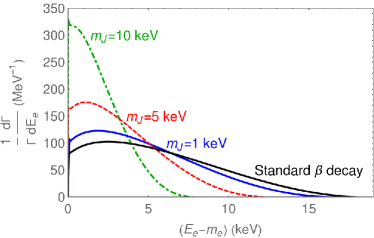
Figure 1: Normalized electron energy spectrum of the decay ${}^{3}\text{H}\to{}^{3}\text{He}^{+}+e^{-}+\bar{\nu}_{e}+J$ (with the pseudoscalar $J$ emitted from the neutrino) and the standard $\upbeta$-decay spectrum. The coupling $g_{\nu J}$ has been set to $1$, the spectrum scales with $g_{\nu J}^{2}$.

Pseudoscalar particles arise in many extensions beyond the Standard Model (SM), especially in those with a complex scalar sector. It is common to find massive CP-even and CP-odd (pseudoscalar) scalar fields in these theories. Axions and axion-like particles also fall into this category. In some cases, these pseudoscalar particles play the role of mediators between SM particles and the dark matter sector. In some other cases, they are connected to neutrino masses and lepton number violation, most notably in so-called Majoron models Chikashige:1980ui ; Schechter:1981cv ; Pilaftsis:1993af ; Garcia-Cely:2017oco . Agnostic to its possible origin, we assume here that the pseudoscalar $J$ is coupled to neutrinos via

$${\cal L}=ig_{\nu J}\,\bar{\nu}\,\gamma_{5}\,\nu\,J\,.$$ (4)

The above coupling is lepton number conserving. As indicated above, there is another possibility, namely a lepton number violating coupling $\bar{\nu}^{c}\gamma_{5}\nu J$. For $\upbeta$-decay there is no difference, while some limits depend on the nature of the coupling, see Sec V. The electron energy spectrum from the decay ${}^{3}\text{H}\to{}^{3}\text{He}^{+}+e^{-}+\bar{\nu}_{e}+J$ is derived in detail in App. A and illustrated in Fig. 1 for various masses. Since analytical expressions are highly cumbersome, we will resort to an excellent approximate expression, given by

$$\frac{\mathrm{d}\Gamma}{\mathrm{d}E_{e}}=\frac{K}{\hbar}\sqrt{\frac{E_{e}}{m_{e}}-1}\,\left(1-\frac{E_{e}}{E_{e}^{\text{max}}}\right)^{n}F(Z,E_{e})\,.$$ (5)

Here, $F(Z,E_{e})$ is the Fermi function, Eq. (38), which describes the interaction of the outgoing electron with the helium nucleus; $K$ is a dimensionless normalization factor and $n$ the spectral index, which is between $2$ and $4.5$ for all our models.

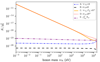
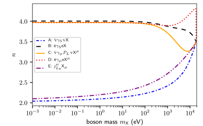
Figure 2: Parameters for the spectrum approximation of Eq. (41) for various coupling structures.

In the case of a pseudoscalar emitted from the outgoing neutrino we find $K\simeq 10^{-25}g_{\nu J}^{2}$ and $n\simeq 2$ for $m_{J}$ around eV, see Fig. 2 for the full $m_{J}$ dependence. This implies branching ratios below $0.1g_{\nu J}^{2}$ with respect to the SM decay rate, as shown in Fig. 3. For larger $J$ masses the branching ratio goes down due to phase-space closure. Note that we find a small logarithmic divergence that arises for small $m_{J}$ due to the emission off of a massless neutrino.

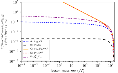
Figure 3: Ratio of the decay width $\Gamma({}^{3}\text{H}\to{}^{3}\text{He}^{+}+e^{-}+\bar{\nu}_{e}+X)$ (divided by the relevant coupling constant $g_{X}^{2}$) with respect to the SM width as a function of the new boson’s mass $m_{X}$. The different curves are for different underlying coupling structures, see text for details.

II.2 Pseudoscalars emitted from electrons

As a second example, consider a pseudoscalar $J$ coupled to electrons. The relevant part of the Lagrangian takes the form

$${\cal L}=ig_{eJ}\,\bar{e}\,\gamma_{5}\,e\,J\,.$$ (6)

This kind of couplings typically appears in axion models or, at least at one-loop, in Majoron models Chikashige:1980ui ; Schechter:1981cv ; Pilaftsis:1993af ; Garcia-Cely:2017oco . A light pseudoscalar can be also part of an extended Higgs sector. We stay agnostic about the origin of $J$ and keep its mass $m_{J}$ and coupling $g_{eJ}$ as free parameters to be determined experimentally.

The resulting electron spectrum can again be extremely well described by the simple function of Eq. (5). For $m_{J}$ below eV, the relevant parameters are $K\simeq 1.4\times 10^{-27}g_{eJ}^{2}$ and $n\simeq 4$. As can be seen from Fig. 3, the resulting branching ratio is rather small even for $g_{eJ}\sim 1$. Note that the amplitude is well-behaved in the limit $m_{J}\to 0$, unlike for the neutrino coupling.

II.3 Vector bosons emitted from neutrinos

An interesting possibility arises via the presence of a light neutral vector boson $Z^{\prime}$. Such bosons are a common feature in many beyond-the-SM frameworks with additional gauge symmetries. Their masses are typically determined by a (combination of) gauge coupling(s) and the energy scale at which the additional gauge symmetry is spontaneously broken Langacker:2008yv , or in some other cases via the Stückelberg mechanism Ruegg:2003ps . Either way, it is conceivable to have light $Z^{\prime}$ bosons, which are subject of intensive studies, for instance if they behave like dark photons Alexander:2016aln . Recent model building perspectives for a light $Z^{\prime}$ coupled to neutrinos can be found in Refs. Farzan:2016wym ; Bakhti:2018avv . We will focus on an effective description of $Z^{\prime}$ interactions with left-handed neutrinos as described by the Lagrangian

$${\cal L}=g_{\nu L}\,\bar{\nu}\gamma^{\mu}P_{L}\nu Z^{\prime}_{\mu}\,.$$ (7)

For $m_{Z^{\prime}}$ below $100\,\mathrm{eV}$, the spectrum is well-described by Eq. (5) with $n\simeq 4$ and $K\simeq 6.7\times 10^{-22}g_{\nu L}^{2}(\mathrm{keV}/m_{Z^{\prime}})^{2}$, see Fig. 2. The decay width shows the characteristic $1/m_{Z^{\prime}}^{2}$ behavior from the longitudinal component of the $Z^{\prime}$, as expected from a coupling to a non-conserved current Dror:2017ehi ; Dror:2017nsg . Note that this is the result of the non-renormalizability of the Lagrangian, i.e. an effective field theory. A full UV-complete theory would eventually correct this feature, which is however a quite model-dependent effect. We assume here that the solution to the $1/m_{Z^{\prime}}^{2}$ behavior does not kick in before the mass scales that Katrin can probe. Nevertheless, the unphysical low mass behavior of this particular model (and the one in the next subsection), illustrates that a measurement at low energies gives crucial information, which is different from extrapolating limits obtained at higher energy scale.

II.4 Vector bosons emitted from electrons

In a similar vein, we assume the following Lagrangian for the coupling of a $Z^{\prime}$ with electrons:

$${\cal L}=\bar{e}\gamma^{\mu}(g_{eL}\,P_{L}+g_{eR}\,P_{R})eZ^{\prime}_{\mu}\,.$$ (8)

In principle one can imagine different couplings for the chiralities, $g_{eL}\neq g_{eR}$, but we will take them to be equal for simplicity, $g_{eL}=g_{eR}\equiv g_{eV}$, corresponding to a vector-like coupling.

For small $m_{Z^{\prime}}$, the spectrum is identical to that of Eq. (7), i.e. with parameters $n\simeq 4$ and $K\simeq 6.7\times 10^{-22}g_{eV}^{2}(\mathrm{keV}/m_{Z^{\prime}})^{2}$, see Fig. 2. This is not surprising upon noting that the electron-number current $j^{\alpha}_{L_{e}}=\bar{\nu}_{e}\gamma^{\alpha}P_{L}\nu_{e}+\bar{e}\gamma^{\alpha}e$ is classically conserved, so a light $Z^{\prime}$ coupled to it would not lead to a $1/m_{Z^{\prime}}^{2}$ divergence (see Sec. II.5). This merely means that the $1/m_{Z^{\prime}}^{2}$ divergence of the $\bar{e}\not{Z^{\prime}}e$ coupling is exactly canceled by the $1/m_{Z^{\prime}}^{2}$ divergence of the $\bar{\nu}_{e}\not{Z^{\prime}}P_{L}\nu_{e}$ coupling.

There are of course differences between the $Z^{\prime}$ coupling to electrons and neutrinos, at least for larger $Z^{\prime}$ masses where the $1/m_{Z^{\prime}}^{2}$ behavior is less dramatic. From Fig. 2 we can see that the two couplings become distinguishable for boson masses above keV.

II.5 Vector bosons emitted from neutrinos and electrons

As mentioned above, a $Z^{\prime}$ that is coupled to the classically conserved electron-number current $j_{L_{e}}$ has a qualitatively different behavior than a $Z^{\prime}$ that only couples to electrons or neutrinos. With

$${\cal L}=g_{L_{e}}\,j^{\alpha}_{L_{e}}Z^{\prime}_{\alpha}=g_{L_{e}}\left(\bar{\nu}_{e}\gamma^{\alpha}P_{L}\nu_{e}+\bar{e}\gamma^{\alpha}e\right)Z^{\prime}_{\alpha}$$ (9)

one finds that the amplitude for $Z^{\prime}$ emission is approximately constant in the limit of small $m_{Z^{\prime}}$, contrary to the two cases discussed above, because $j^{\alpha}_{L_{e}}$ is a classically conserved (non-anomalous) current. Fitting to the approximate spectrum gives $n\simeq 2.2$ and $K\simeq 5\times 10^{-24}g_{L_{e}}^{2}$ for $m_{Z^{\prime}}\sim\mathrm{eV}$, see Fig. 2. Similar to the scalar-neutrino case there is still a logarithmic dependence on $m_{Z^{\prime}}$ that is well known from Bremsstrahlung in QED. For larger $m_{Z^{\prime}}\gtrsim 10\,\mathrm{keV}$, the behavior becomes identical to that of a $Z^{\prime}$ coupled to neutrinos.

III $\mathrm{eV}$-scale light bosons in the current Katrin setup

In order to compare the theoretical prediction for the light bosons to upcoming data taken by the Katrin experiment in the current setting, we will apply several modifications to the analytical form given in Eq. (5) to account for experimental characteristics. We will refer to this as the experimental spectrum. In the following, we will introduce the modifications to the spectrum before stating the sensitivity of Katrin to constrain the emission of a light boson in tritium -decay. For better readability and overview, we summarize the possible production mechanisms in Tab. 1 which we will later refer to when stating the results.

Mechanism	$K/g_{X}^{2}$	$n$
A: Pseudoscalars from neutrinos	$10^{-25}$	2
B: Pseudoscalars from electrons	$10^{-27}$	4
C: Vector bosons from neutrinos	$7\cdot 10^{-16}(\text{eV}/m_{X})^{2}$	4
D: Vector bosons from electrons	$7\cdot 10^{-16}(\text{eV}/m_{X})^{2}$	4
E: Vector bosons from both	$5\cdot 10^{-24}$	2

Table 1: Different production mechanisms. This table gives an overview about the different production mechanisms for the light boson $X$ and their effect on the spectrum, caused by different forms for $K$ and $n$. The values stated are approximations for eV-scale light bosons.

III.1 Experimental characteristics

Since Katrin employs gaseous molecular tritium ($\text{T}_{2}$), we have to use the molecular masses to calculate the endpoint:

$$E_{e}^{\text{max}^{\prime}}=\frac{m^{2}_{\text{T}_{2}}-(m_{\text{T}\,^{3}\text{He}^{+}}+m_{\upnu}+m_{X})^{2}+m_{e}^{2}}{2m_{\text{T}_{2}}}\,,$$ (10)

which for $m_{\upnu}=m_{X}=0$ gives $E_{e}^{\text{max}^{\prime}}=$18575\text{\,}\mathrm{eV}$+m_{e}$.

Switching to kinetic electron energy $E=E_{e}-m_{e}$ instead of total electron energy $E_{e}$ results in

$$\frac{\text{d}\Gamma}{\text{d}E}=\frac{K}{\hbar}\sqrt{\frac{E}{m_{e}}}\left(\frac{E_{\text{max}}-E}{E_{\text{max}}+m_{e}}\right)^{n}F(Z,E)\,,$$ (11)

with

$$\begin{split}E_{\text{max}}&=E_{e}^{\text{max}^{\prime}}-m_{e}-(m_{\upnu}+m_{X})\\ &=E_{0}-(m_{\upnu}+m_{X})\,.\end{split}$$ (12)

The spectra of the 5 different cases, together with the standard -decay spectrum for different neutrino masses, are plotted in Fig. 4.

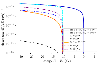
Figure 4: Differential spectrum - Shown are 7 different cases: standard -decay without (solid blue) and with $10\text{\,}\mathrm{eV}$ (dashed cyan) neutrino mass, as well as the 5 spectra as expected for the additional emittance of a light boson $X$ with $g_{X}=1$, $m_{X}=$10\text{\,}\mathrm{eV}$$ with type according to Tab. 1. (Legend: dash dotted blue - A, dashed black - B, solid orange/dotted red - C/D, dash dotted dotted magenta - E.)

The detailed modeling of the decay spectrum requires several modifications to the analytical description Kleesiek:2018mel , leading to

$$\frac{\text{d}\Gamma}{\text{d}E} =\frac{K}{\hbar}\sqrt{\frac{E}{m_{e}}}\,F(Z,E)$$ (13)

$$\quad\times\sum_{fs}P_{fs}\cdot f_{\text{rad}}(E-E_{fs})\cdot\left(\frac{E_{\text{max, fs}}-E}{E_{\text{max, fs}}+m_{e}}\right)^{n},$$

whose factors will be discussed briefly in this section.

Radiative corrections:

Due to interaction with virtual and soft real photons in the Coulomb field of the nucleus, the emitted electrons lose energy. This loss is accounted for by the correction factor $f_{\text{rad}}(E-E_{fs})$ in Eq. (13), as recommended in Ref. Repko:1984cs .

Molecular recoil:

As discussed in the Katrin design report Angrik:2005ep , in the region around the endpoint the electron energy dominates over the neutrino energy. Therefore, the recoil energy of the molecule balances the momentum of the electron:

$$E_{\text{rec}}\approx E\cdot\frac{m_{e}}{m_{{}^{3}\text{HeT}^{+}}}\,.$$ (14)

We include this $1.7\text{\,}\mathrm{eV}$ shift into the final states distribution Kleesiek:2018mel .

Final states:

Katrin is using a molecular tritium source, which contains several tritiated hydrogen isotopologues. Those are T₂, DT and HT which decay into (³HeT)⁺, (³HeD)⁺ and (³HeH)⁺. The dominant isotopologue will be T₂, due to the tritium purity $\epsilon_{\text{T}}>0.95$. The decay may leave the daughter molecule in a rovibronic (rotational and vibrational) or electronic excited final state. Distributions of these excited states were calculated by Saenz and others Saenz:2000dul ; Doss:2006zv ; Doss2008 and are quantified in terms of excitation energy $E_{fs}$ and the corresponding probability $P_{fs}$. The final states energy $E_{fs}$ reduces the maximum energy of the electron: Eq. (12) thus becomes

$$E_{{\rm max},fs}=E_{0}-E_{fs}-(m_{\upnu}+m_{X})\,,$$ (15)

requiring the summation of the decay rate over all possible final states $fs$ in Eq. (13).

Doppler effect:

The tritium molecules in the source are at a non-zero temperature of $30\text{\,}\mathrm{K}$, which causes thermal motion. This thermal motion together with the bulk velocity of the gas flow is called Doppler effect and causes a Gaussian broadening of the electron energy spectrum of about $100\text{\,}\mathrm{meV}$ Kleesiek:2018mel .

III.2 Combination with standard -decay spectrum

We define the form of the overall spectrum as

$$\frac{\text{d}\Gamma}{\text{d}E}=\left.\frac{\text{d}\Gamma}{\text{d}E}\right|_{\upbeta}+\left.\frac{\text{d}\Gamma}{\text{d}E}\right|_{X}.$$ (16)

Fig. 5 shows the superposition of a light boson of type A (large coupling $g_{\nu J}=5$ assumed for visualization) for $m_{J}=$10\text{\,}\mathrm{eV}$$ and of the standard -spectrum with vanishing neutrino mass. Note that the common normalization parameter ensures that the decay activity stays constant.

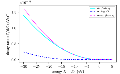
Figure 5: Combination with standard -decay - Shown is the signature of a light boson of type A with $g_{\nu J}=5$, $m_{J}=$10\text{\,}\mathrm{eV}$$ together with standard -decay spectrum with vanishing neutrino mass.

Katrin measures an integrated spectrum with the high voltage $U$ at the main spectrometer acting as a high-pass filter Angrik:2005ep . Using the concept of a response function $R(E,qU)$ Angrik:2005ep ; Kleesiek:2018mel , the measured spectrum can be written as

$$\dot{N}\propto\int_{qU}^{\infty}R(E,qU)\left(\left.\frac{\mathrm{d}\Gamma}{\mathrm{d}E}\right|_{\upbeta}+\left.\frac{\mathrm{d}\Gamma}{\mathrm{d}E}\right|_{X}\right)\mathrm{d}E\,.$$ (17)

III.3 Settings

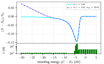
Figure 6: Relative change of the integrated spectrum - Shown is the neutrino mass sensitive region by comparing a spectrum with neutrino mass $m_{\upnu}=$1\text{\,}\mathrm{eV}$$ to a spectrum without neutrino mass (solid cyan). The peak of the measuring time distribution sits right in the region where the neutrino mass causes the largest distortion to the spectrum. Furthermore the signal of a light boson type A with $g_{\nu J}=5$, $m_{X}=$10\text{\,}\mathrm{eV}$$ additional to the massive neutrino is compared to the null-hypothesis (dash dotted blue).

The light boson spectrum superimposed to the standard -decay spectrum has 6 fit parameters:

1. neutrino mass squared $m_{\upnu}^{2}$

2. endpoint $E_{0}$

3. amplitude $Amp$ which is a factor ensuring correct normalization of the superposition of light boson and standard -decay spectrum

4. background rate $Bg$

5. light boson mass $m_{X}$

6. light boson coupling $g_{X}$

In the following we use the standard settings defined in the design report Angrik:2005ep . This includes a measuring window of high voltage values ranging in the interval $[E_{0}-$30\text{\,}\mathrm{eV}$,E_{0}+$5\text{\,}\mathrm{eV}$]$ (see Fig. 6), a true neutrino mass of zero and a measuring time of three years.

III.4 Statistical sensitivity

Here we state statistical sensitivity estimates for the potential of Katrin to constrain the emittance of a light boson additional to the standard -decay. Estimation of confidence intervals in the presence of nuisance parameters $\pi$ can easily lead to errors, for instance if one neglects correlations between the nuisance parameters and the parameters of interest $\Theta$. Thereby, errors on parameters of interest may be underestimated.

To minimize this risk, we will make use of the so-called profile likelihood method Rolke:2004mj . Using a likelihood ratio test statistic which converges to a $\chi^{2}$ random variable, we can extract confidence limits from the likelihood function similar to the $\chi^{2}$ method. We define the profile likelihood

$$L_{p}(\Theta)=L(\Theta,\hat{\pi}(\Theta))$$ (18)

with $\hat{\pi}(\Theta)$ being the function that maximizes the likelihood with respect to its nuisance parameters $\pi$. The profile likelihood therefore only depends on the parameters of interest $\Theta$. Using the best-fit estimate $\hat{\Theta}$, we define the likelihood ratio test statistic

$$\lambda(\Theta)=\frac{L_{p}(\Theta)}{L_{p}(\hat{\Theta})}\,.$$ (19)

Now we can scan the profile likelihood to find the values of $\Theta$ where Eq. (18) increases by a specific factor. For example to find the $1\sigma$ intervals of a single parameter $\Theta$ one would search for $\Theta$ where $-2\Delta\log L_{p}(\Theta)=-2\log\lambda=1$.

In our case, we have two parameters of interest, namely the coupling $g_{X}$ and the mass of the light boson $m_{X}$. To determine the sensitivity, we compare our likelihood for non-vanishing $g_{X}$ and $m_{X}$ against the null-hypothesis of no light boson: for every point in the 2-dim grid of ($g_{X}$, $m_{X}$) we minimize the likelihood with respect to the nuisance parameters $m_{\upnu}^{2}$, $E_{0}$, $Amp$ and $Bg$. We then can find the likelihood ratios corresponding to 90 % C.L. The resulting sensitivity curve for pseudoscalar bosons is shown in Fig. 7 and for vector bosons in Fig. 8.

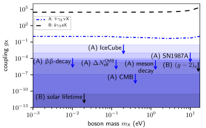
Figure 7: Statistical sensitivity contours for eV-scale light pseudoscalar bosons - Shown is the 90 % C.L. statistical sensitivity of Katrin for the detection of eV-scale light pseudoscalar bosons. The types A, B are defined according to Tab. 1. Furthermore, the shaded areas mark the parameter regions allowed from constraints discussed in Sec. V.

(A) Pseudoscalars emitted from neutrinos:

Here we expect best sensitivity with increasing coupling $g_{\nu J}$ due to the form of the spectrum (compare Tab. 1 and Eq. (11)): the factor $K$ is proportional to $g_{\nu J}^{2}$. As can be seen from Fig. 7, this expectation is confirmed. Also we can see that the sensitivity decreases again for masses larger than $10\text{\,}\mathrm{eV}$: the mass limit is constrained by the extent of the measuring time Katrin is using to scan the spectrum. Masses larger than $30\text{\,}\mathrm{eV}$ are not accessible in this study due to the used measuring time distribution (compare Fig. 6), however, there is a small increase in sensitivity for boson masses around $1\text{\,}\mathrm{eV}$.

(B) Pseudoscalars emitted from electrons:

As mentioned in the beginning, this production mechanism for the light bosons is expected to be suppressed compared to the others due to the small branching ratio. Nevertheless Fig. 7 shows the expected sensitivity of Katrin towards this light boson type B. As expected, large couplings $g_{eJ}$ are required in order for Katrin to be sensitive towards this kind of boson.

(C, D) Vector bosons emitted from neutrinos or electrons:

For the production mechanisms C and D (which electron spectra look exactly the same for eV-scale bosons), we expect an inverted behavior for low couplings compared to case A: electron spectra coupled to bosons of type C and D have a $1/m_{Z^{{}^{\prime}}}^{2}$ divergence in their $K$. Therefore, small boson masses are strongly favored in this case. This should lead to higher sensitivity of Katrin for smaller boson masses. Exactly this behavior can be seen from Fig. 8: C and D in contrast to A and B have good sensitivity towards lower boson masses.

(E) Vector bosons emitted from neutrinos and electrons:

For production mechanism E, we have spectrum parameters similar to A (compare Tab. 1) and therefore expect a similar sensitivity curve. Fig. 8 confirms this expectation: the best sensitivity is expected for a light boson mass around $1\text{\,}\mathrm{eV}$.

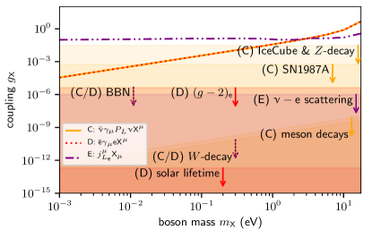
Figure 8: Statistical sensitivity contours for eV-scale light vector bosons - Shown is the 90 % C.L. statistical sensitivity of Katrin for the detection of eV-scale light vector bosons. The types C, D, E are defined according to Tab. 1 (C and D are indistinguishable for eV-scale vector bosons). Furthermore, the shaded areas mark the parameter regions allowed from constraints discussed in Sec. V.

It has to be noted that we conducted this study for each type of light boson separately. In the final analysis, only the most physically relevant case might be considered. Furthermore, we want to stress that this study might additionally be evaluated with possible eV-sterile neutrino mass and mixing angle as additional nuisance parameters. It was also checked that moderate constraints on the coupling of the light bosons are enough to not impact the Katrin neutrino mass sensitivity in the light boson scenario at hand. For example, a conservative constraint on the coupling of boson type E to values below $1$ preserves the Katrin neutrino mass sensitivity of $200\text{\,}\mathrm{meV}$. In order to derive the final experimental sensitivity for the different cases, systematic effects as described in Angrik:2005ep need to be evaluated with respect to each specific spectrum.

IV $\mathrm{keV}$-scale light bosons: statistical sensitivity

Following the study in Ref. Mertens:2014nha we consider a measurement of the complete differential -decay spectrum at the Katrin experiment with a new detector and readout system. In this case it is the detector itself which determines the electron energy. The main spectrometer is kept at a small retarding potential to allow electrons from most of the spectrum to reach the detector. A new detector system is needed to handle much higher count rates in the whole spectrum as compared to the endpoint region, provide better energy resolution, and limit several systematic effects that arise when measuring the full -spectrum.

As a case study of expected statistical sensitivity to the light boson coupling constant $g_{X}$ and mass $m_{X}$ we consider the differential measurement with the design Katrin setup but modified detector system for a duration of three years. The corresponding total statistics amounts to about $10^{18}$ electrons. Furthermore, we assume for the energy resolution a conservative full width at half maximum of $300\text{\,}\mathrm{eV}$, based on recent evaluation of the detector prototype Mertens:2018 , and constant background rate of $2\text{\,}\mathrm{mcps}\text{\,}{\mathrm{keV}}^{-1}$, based on measurements with the existing detector at the Katrin setup Harms:2015 . Evidently, for $\mathrm{keV}$-scale boson the normalization prefactor $K$ and spectral index $n$ are no longer constants and must be considered as functions of the boson mass, see Fig. 2.

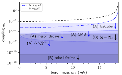
Figure 9: Purely statistical sensitivity contours for $\mathrm{keV}$-scale light pseudoscalar bosons - Shown is the $90\text{\,}\mathrm{\char 37\relax}$ C.L.  statistical sensitivity of a Katrin differential spectrum measurement with a new detector system. Furthermore, the shaded areas mark the parameter regions allowed from constraints discussed in Sec. V.

Using the profile likelihood method similarly as in Sec. III we obtain the $90\text{\,}\mathrm{\char 37\relax}$ C.L. sensitivity curves in Figs. 9 and 10. In the study we have assumed a Gaussian pull term on the neutrino mass with a width of $2\text{\,}\mathrm{eV}$. The sensitivity drops significantly for larger boson masses as expected due to the decreasing decay width of the light boson relative to the SM width. As in the $\mathrm{eV}$-scale case the branching ratio is generally small for the pseudoscalar emitted from electrons (type B), leading to relatively worse sensitivity with respect to the other production mechanisms. For vector bosons emitted either from neutrinos (C) or electrons (D) the sensitivity increases significantly for low masses due to the $1/m_{Z^{{}^{\prime}}}^{2}$ behavior of the decay width. Furthermore, the similar experimental sensitivity reflects the similarity of the spectrum of vector boson emitted from electrons (D) to that from neutrinos (C) for small masses as well as the spectrum of vector boson emitted from both electrons and neutrinos (E) to that from neutrinos (C) for larger masses.

The huge statistics available from tritium -decay in a Katrin-like experiment allows probing the $\mathrm{keV}$-scale boson coupling constant to as low as $g_{X}^{2}\sim 10^{-8}$ for some of the models. Nevertheless, as already recognized for the $\mathrm{keV}$-scale sterile neutrino in Ref. Mertens:2018 the final experimental sensitivity will be limited by unavoidable systematic effects connected to observing the entire -spectrum. Detailed studies are thus required in order to assess the final experimental sensitivity. Besides, the presented statistical sensitivity is valid when the experimental search is done for a given most physically relevant type of particle.

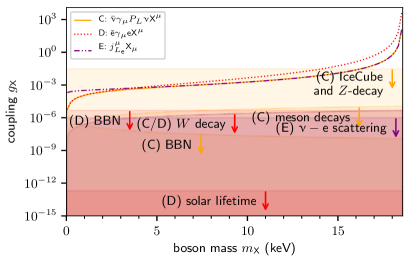
Figure 10: Purely statistical sensitivity contours for $\mathrm{keV}$-scale light vector bosons - Shown is the $90\text{\,}\mathrm{\char 37\relax}$ C.L.  statistical sensitivity of a Katrin differential spectrum measurement with a new detector system. Furthermore, the shaded areas mark the parameter regions allowed from constraints discussed in Sec. V.

V Additional bounds on light states

New light states are actively searched for at laboratory scales also through different processes with respect to the one considered in this work. Moreover, their interactions sensibly affect cosmological and astrophysical processes. This leads to potentially very strong bounds on the strength of their interaction affecting the expected sensitivity region for the Katrin experiment. Below we briefly illustrate and discuss the most relevant bounds for the scenarios under consideration.

Concerning possible complementary or competitive laboratory constraints, we have first of all to consider the emission of light bosons in the decays of the $Z$, $W$, and of light charged mesons $P$, hence leading to three-body decay processes like $Z\rightarrow\nu\nu X$, $W\rightarrow e\nu X$ and $P\rightarrow e\nu X$. Three-body decay rates of the $Z$ and $W$ bosons are strongly constrained by the very precise measurements of their total decay widths, while the decay rate of the mesons are probed by dedicated searches. In the case of models C and E we consider the bound reported in Laha:2013xua on the $Z\rightarrow\nu\nu X$ process, which can be approximately expressed as $g_{\nu L},g_{L_{e}}\lesssim 3\times 10^{-2}$. Concerning $W$ decay, the cases of models $C/D$ and $E$ are very different. For the former, similarly to what occurs in the model presented in Laha:2013xua , the $Z^{{}^{\prime}}$ is coupled to an anomalous current of SM leptons, leading to a $1/m_{Z^{\prime}}^{2}$ enhancement of the three body decay rate of the $W$, determining the very strong bound:

$$g_{eV},g_{\nu L}\lesssim 2.5\times 10^{-7}\left(\frac{m_{Z^{\prime}}}{1\,\mathrm{keV}}\right).$$ (20)

Note that we need to extrapolate this bound to low masses in order to apply it to our scenario. Model E, on the contrary, does not feature this anomalous coupling, hence the decay rate of $W\rightarrow e\nu Z^{{}^{\prime}}$ depends only logarithmically on $m_{Z^{\prime}}$ and gives a weaker limit as the one from $Z\rightarrow\nu\nu Z^{{}^{\prime}}$. Bounds from light meson decays applicable to model C have been considered in Bakhti:2017jhm . For our study we will adopt the bound from the process $\pi\rightarrow e\nu Z^{{}^{\prime}}$:

$$g_{\nu L}\lesssim 6\times 10^{-7}\left(\frac{m_{Z^{\prime}}}{1\,\mathrm{keV}}\right).$$ (21)

Slightly stronger bounds would be obtained from violation of lepton universality Bakhti:2017jhm ; Bakhti:2018avv . These would be, however, dependent on eventual couplings of the light vector with second generation leptons. According to an analogous reasoning as for the case of $W$ decays, Eq. (21) cannot be applied to model E, since the $1/m_{Z^{\prime}}^{2}$ enhancement of the decay rate would not be present.

Limits applicable to model A from decays of light mesons have been provided in Pasquini:2015fjv (see also Lessa:2007up ; Albert:2014fya ). For our analysis we will adopt the constraint $g_{\nu J}<4.4\times 10^{-5}$, independent on the mass of the pseudoscalar $J$ for the whole range of masses considered in this work.

Models B, D and E are also constrained by the determination of the anomalous magnetic moment of the electron Tanabashi:2018oca ; Parker191 . The corresponding upper bounds read Lindner:2016bgg ; Liu:2018xkx :

$$\begin{split}&g_{eJ}\lesssim 1.8\times 10^{-5}\,,\\ &g_{eV}\lesssim 4.0\times 10^{-6}\,\end{split}$$ (22)

for the cases of a pseudoscalar (model B) and vector (models D and E) boson, respectively. As evident, the limit is stronger in the case of vector bosons. This is due to the fact that the corresponding contribution to $(g-2)_{e}$ adds to the SM one, in tension with the slight experimental evidence towards a negative deviation of the anomalous magnetic moment of the electron with respect to the SM expectation.

In scenario E a strong bound $g_{eV}\lesssim 10^{-6}$ Laha:2013xua ; Lindner:2018kjo arises from electron-neutrino scattering.

We finally remark that, in the case of a lepton number violating coupling, constraints from neutrinoless double beta decay, determined in Majoron models, can be applied to model A. These can be expressed as an upper bound on the coupling $g_{\nu J}$ of the order $10^{-4}$ to $10^{-5}$ Blum:2018ljv ; Brune:2018sab .

Together with these laboratory limits, cosmological and astrophysical constraints should be considered as well.

Concerning astrophysical constraints, very strong ones apply to models B and D. Indeed, a boson $X$ coupled to an electron pair would be responsible for energy loss in the interior of stars as a consequence of Bremsstrahlung ($e+Ze\rightarrow Ze+e+X$) and Compton ($\gamma+e\rightarrow e+X$) processes. The corresponding cross sections have been determined for the models B and D, for example, in Gondolo:2008dd (this bound has been also revised in Redondo:2008aa ; An:2013yfc for dark photon models, potentially applicable to model D). The requirement of not altering the properties of the Sun translates into the strong constraint $g_{eJ}\lesssim 3\times 10^{-11}$ for the case of a boson with pseudoscalar coupling to electrons (model B) and an even stronger upper bound $g_{eV}\lesssim 2\times 10^{-13}$ in the case of a boson with vectorial coupling (model D). Notice that this bound implicitly assumes that the new state is capable of escaping the Sun. It is conceivable that, for strong enough coupling, it gets instead trapped within the Sun and reprocessed back into SM states without causing energy loss. An assessment of this effect would, however, require a dedicated study which is beyond the scope of this paper.

Bounds on the interactions of a new light state with neutrinos come from the observed flux of neutrinos from galactic and extragalactic sources. In the presence of a light mediator, high-energy or ultra-high energy neutrinos would feature an enhanced scattering rate on the Cosmic Neutrino Background (C$\nu$B) implying reduced fluxes, with respect to SM expectations, at Earth. Along this way of reasoning the pioneering work Kolb:1987qy provided limits on the interactions of the neutrinos with a light boson based on the observation of neutrinos from the supernova SN1987A. This reference considered the cases of a very light spin-1 mediator (relevant for eV states in model C), a massive spin-1 mediator (keV states in model C) and a Majoron (relevant for eV states in model A) obtaining, respectively, the limits $g_{\nu L}\lesssim 5.6\times 10^{-4}$, $g_{\nu L}/m_{Z^{\prime}}<12/\mathrm{MeV}$ and $g_{\nu J}\lesssim 10^{-3}$. According to a similar logic, Refs. Ng:2014pca ; Ioka:2014kca considered the case of the flux of extragalactic neutrinos measured by IceCube. In particular Ref. Ioka:2014kca provided the limit $g_{X}\lesssim 0.03$ which can be applied to both models A and C for all the ranges of masses considered in our study.

New light states coupled to neutrinos can also be efficiently produced in core-collapse supernovae environments and affect their evolution. Since the observed flux of neutrinos from SN1987A was compatible with standard predictions, it is possible to obtain constraints on the coupling of the new states with neutrinos. Studies along this line have been performed mostly in the context of Majoron models, see e.g. Gelmini:1982rr ; Choi:1987sd ; Berezhiani:1989za ; Choi:1989hi ; Chang:1993yp ; Kachelriess:2000qc ; Tomas:2001dh ; Lindner:2001th ; Hannestad:2002ff ; Farzan:2002wx ; Fogli:2004gy ; Das:2011yh ; Brune:2018sab ; extensions to more generic scalar and pseudoscalar states have been considered in Heurtier:2016otg ; Farzan:2018gtr . As a consequence of this we will consider supernova bounds in the context of model A.

The environment of supernova cores is affected in different ways by the presence of light BSM states interacting with neutrinos. First of all, the production process $\nu\nu\rightarrow J$ leads to energy depletion, hence reducing the neutrino flux, and to deleptonization (i.e. reduction of the electron lepton number inside the supernova core), eventually preventing the explosion of the supernova. These two effects should be considered, however, only if the interactions of the state $J$ are feeble enough that it can escape the supernova core. On the contrary, for $g_{\nu J}\gtrsim 10^{-5}$, the scattering processes $\nu+J\rightarrow\nu+J$ are efficient enough to trap the $J$ particles inside the supernova core, so that they eventually decay back into neutrinos such that no energy loss or deleptonization occurs. As evident from Figs. 7 and 9 the region of interest of Katrin lies in the trapping regime for the state $J$ and hence the constraints just mentioned do not apply in our scenario.

Moving finally to cosmological constraints, light states with sizable interactions with neutrinos can contribute to the effective number of the neutrino species, $N_{\rm eff}$, which is constrained both by Big Bang Nucleosynthesis (BBN) and the Cosmic Microwave Background (CMB). BBN bounds are relevant only in the case of a vector boson; a (pseudo)scalar state, even if fully in thermal equilibrium at the time of BBN, would contribute to the effective number of neutrinos by an amount of at most $\Delta N_{\rm eff}\approx 0.57$, well compatible with the bound $\Delta N_{\rm eff}<1$ Mangano:2011ar . On the contrary a vector boson, because of the larger number of degrees of freedom, can contribute up to $\Delta N_{\rm eff}=1.71$. A simple estimate of the BBN bound, for model C, can be obtained by requiring that the relevant interaction rate of the new state with the neutrinos is below the Hubble expansion rate at the typical temperature of BBN, $T\sim 1\,\mathrm{MeV}$. For a keV mass state the most relevant interaction is the inverse decay $\nu\nu\rightarrow Z^{\prime}$. In such a case the BBN constraint is translated into an upper bound on the coupling of the form Ahlgren:2013wba ; Huang:2017egl

$$g_{\nu L}\lesssim 2.2\times 10^{-7}\left(\frac{1\,\mathrm{keV}}{m_{Z^{\prime}}}\right).$$ (23)

In the case of an eV state one should instead consider the neutrino annihilation processes $\nu\nu\rightarrow Z^{\prime}Z^{\prime}$ which yields the bound Huang:2017egl

$$g_{\nu L}\lesssim 4.6\times 10^{-6}\,.$$ (24)

While these estimates are already a very good approximation, we have adopted the more refined limits determined in Huang:2017egl for our analysis. A similar way of reasoning could also be applied for the limits on measurements of $N_{\rm eff}$ at the CMB time. The stronger constraint $\Delta N_{\rm eff}<0.3$ at $95\%$  C.L. Aghanim:2018eyx allows to probe also model C. As discussed for example in Boehm:2012gr , a quantitative assessment on the contribution to $\Delta N_{\rm eff}$ depends on the details of the decoupling of the light state from neutrinos and is beyond the purpose of this work. In Figs. 7 and 9 we report the contour corresponding to the case of decoupling at temperatures of the order of MeV, corresponding, as already pointed out, to $\Delta N_{\rm eff}^{\rm CMB}\simeq 0.57$, which is in $2\sigma$ tension with the experimental limit.

Analogous bounds to the ones just discussed can be applied to models B and D. In such a case the eventual equilibration of the new boson $X$ with the thermal SM bath is mostly determined by the rates of $XX\leftrightarrow e^{+}e^{-}$ processes. The condition for the equilibration of this rate is described in a good approximation by Eq. (24). We notice, anyway, that due to the kinematical suppression of the $XX\rightarrow e^{+}e^{-}$ rate from the mass of the electron, the $X$ states would decouple at latest at temperatures of the order of the mass of the electron, $0.5\,\mathrm{MeV}$.

Turning to the CMB, new light states would enhance neutrino self-interactions, implying an alteration of their free-streaming length which would result in an enhancement of the CMB temperature power spectrum at multipoles $l\gtrsim 200$ Hannestad:2004qu ; Bell:2005dr ; Cyr-Racine:2013jua . This effect is customarily analyzed in two limiting regimes. The first one holds if the mass of the mediator is significantly above the typical energy of neutrinos at CMB time (which is around eV). In such a case the only relevant processes are neutrino self-scattering processes, $\nu\nu\rightarrow\nu\nu$, which can be described through an effective four-fermion interaction with coupling $G_{X}=g_{X}^{2}/m_{X}^{2}$. Constraints on these effective couplings have been determined in Cyr-Racine:2013jua ; Archidiacono:2013dua and more recently revised in Lancaster:2017ksf ; Oldengott:2017fhy . As can be easily argued, the case of a keV state falls in this regime. We will apply the following bound, for both models A and C Archidiacono:2013dua :

$$G_{X}\leq 2.5\times 10^{7}\,G_{F}\,,$$ (25)

($G_{F}$ being the Fermi constant), which can be re-expressed as:

$$g_{X}\lesssim 1.2\times 10^{-2}\left(\frac{m_{X}}{1\,\mathrm{MeV}}\right).$$ (26)

The second regime holds for a mediator which can be regarded as massless with respect to the energy of neutrinos at CMB. In such a case a larger variety of processes, including also neutrino annihilations into mediator pairs, should be considered. A study along these lines has been presented e.g. in Ref. Archidiacono:2013dua (see also Forastieri:2015paa ) in the case of a light pseudoscalar (model A) and the very strong bound $g_{\nu J}\lesssim 1.2\times 10^{-7}$ has been obtained.

From the discussion above it is evident that the case of an eV state is troublesome since it does not fit any of these two regimes, since its mass of the same order as the energy of neutrinos at CMB. To our best knowledge, no limit is available for an ${\cal O}(\mathrm{eV})$ mass boson.

Model A: $ig_{\nu J}\,\bar{\nu}\,\gamma_{5}\,\nu\,J$
Double $\beta$ decay (only LNV)	$g_{\nu J}\lesssim 10^{-(4\div 5)}$ Blum:2018ljv ; Brune:2018sab
Meson decays	$g_{\nu J}\lesssim 4.4\times 10^{-5}$ Pasquini:2015fjv
CMB	$g_{\nu J}\lesssim 1.2\times 10^{-2}\left(\frac{m_{J}}{1\,\mathrm{MeV}}\right)\,\,\left(m_{J}\gg 1\,\mathrm{eV}\right)$
	$g_{\nu J}\lesssim 1.2\times 10^{-7}\,\,\left(m_{J}\ll 1\,\mathrm{eV}\right)$ Archidiacono:2013dua
Supernova 1987A	$g_{\nu J}\lesssim 10^{-3}\,\,\left(m_{J}\leq{\cal O}(1\,\mathrm{eV})\right)$ Kolb:1987qy
IceCube	$g_{\nu J}\lesssim 0.03$ Ioka:2014kca
$\Delta N_{\rm eff}^{\rm CMB}$	$g_{\nu J}\lesssim 1.6\times 10^{-6}\left(\frac{1\,\mathrm{keV}}{m_{J}}\right)\,\,\,(m_{J}\simeq{\cal O}(\mathrm{keV}))$
	$g_{\nu J}\lesssim 5\times 10^{-5}\,\,\,(m_{J}\simeq{\cal O}(\mathrm{eV}))$ Huang:2017egl ; Aghanim:2018eyx
Model B: $ig_{eJ}\,\bar{e}\,\gamma_{5}\,e\,J$
Solar lifetime	$g_{eJ}\lesssim 3\times 10^{-11}$ Gondolo:2008dd
$\Delta N_{\rm eff}^{\rm BBN}$	$g_{eJ}\lesssim 5\times 10^{-5}$ Huang:2017egl ; Aghanim:2018eyx
$(g-2)_{e}$	$g_{eJ}\lesssim 1.8\times 10^{-5}$ Parker191 ; Liu:2018xkx
Model C: $g_{\nu L}\,\bar{\nu}\gamma^{\mu}P_{L}\nu Z^{\prime}_{\mu}$
$Z$ decay	$g_{\nu L}\lesssim 3\times 10^{-2}$ Laha:2013xua
$W$ decays	$g_{\nu L}\lesssim 2.5\times 10^{-7}\left(\frac{m_{Z^{\prime}}}{1\,\mathrm{keV}}\right)$ Laha:2013xua
Meson decays	$g_{\nu L}\lesssim 6\times 10^{-7}\left(\frac{m_{Z^{\prime}}}{1\,\mathrm{keV}}\right)$ Bakhti:2017jhm ; Bakhti:2018avv
$\Delta N_{\rm eff}^{\rm BBN}$	$g_{\nu L}\lesssim 2.2\times 10^{-7}\left(\frac{1\,\mathrm{keV}}{m_{Z^{\prime}}}\right)\,\,\left(m_{Z^{\prime}}\simeq{\cal O}(\mathrm{keV})\right)$
	$g_{\nu L}\lesssim 4.6\times 10^{-6}\,\,\left(m_{Z^{\prime}}\simeq{\cal O}(\mathrm{eV})\right)$ Huang:2017egl
CMB	$g_{\nu L}\lesssim 1.2\times 10^{-2}\left(\frac{m_{Z^{\prime}}}{1\,\mathrm{MeV}}\right)\,\,\left(m_{Z^{\prime}}\gg 1\,\mathrm{eV}\right)$ Archidiacono:2013dua
Supernova 1987A	$g_{\nu L}\lesssim 12\left(\frac{m_{Z^{\prime}}}{1\,\mathrm{MeV}}\right)\,\,\left(m_{Z^{\prime}}\geq 60\,\mathrm{eV}\right)$
	$g_{\nu L}\lesssim 5.6\times 10^{-4}\,\,\left(m_{Z^{\prime}}<60\,\mathrm{eV}\right)$ Kolb:1987qy
IceCube	$g_{\nu L}\lesssim 0.03$ Ioka:2014kca
Model D: $g_{eV}\bar{e}\gamma^{\mu}eZ^{\prime}_{\mu}$
$W$ decays	$g_{eV}\lesssim 2.5\times 10^{-7}\left(\frac{m_{Z^{\prime}}}{1\,\mathrm{keV}}\right)$ Laha:2013xua
Solar lifetime	$g_{eV}\lesssim 2\times 10^{-13}$ Gondolo:2008dd
$\Delta N_{\rm eff}^{\rm BBN}$	$g_{eV}\lesssim 4.6\times 10^{-6}$ Huang:2017egl
$(g-2)_{e}$	$g_{eV}\lesssim 4.0\times 10^{-6}$ Parker191 ; Liu:2018xkx
Model E: $g_{L_{e}}\left(\bar{\nu}_{e}\gamma^{\mu}P_{L}\nu_{e}+\bar{e}\gamma^{\mu}e\right)Z^{\prime}_{\mu}$
$Z$ decay	$g_{L_{e}}\lesssim 3\times 10^{-2}$ Laha:2013xua
$\Delta N_{\rm eff}^{\rm BBN,\,CMB}$	as models C and D
$\nu$–$e$ scattering	$g_{L_{e}}\lesssim 10^{-6}$ Laha:2013xua ; Lindner:2018kjo

Table 2: Summary table including all the laboratory, astroparticle, and cosmological constraints which apply to the models considered in this work; LNV $=$ lepton number violating coupling.

The set of constraints discussed in this section is summarized in Tab. 2. Their impact on the sensitivity of the Katrin  experiment, on the various models, is shown in Figs. 7 (9) and 8 (10), respectively for the cases of scalar (models A and B) and vector (models C, D and E) new states with masses $\leq{\cal O}(\mathrm{eV})$ (${\cal O}(\mathrm{keV})$).

As evident, for all the considered scenarios, the sensitivity region of the Katrin  experiment appears to be already excluded by other laboratory searches as well by cosmology and astrophysical observations. We notice, nevertheless, that most of the laboratory constraints here listed have been extrapolated from searches of heavier states. In addition, the energy scale of the processes was orders of magnitude larger than the one of tritium decay. In this regard, the Katrin  detector, which is designed for the search of very light states, would then provide a more solid and complementary constraint. Along a similar reasoning, it would provide a laboratory complement to the astrophysical and cosmological limits, which rely on specific hypotheses.

VI Conclusion

In this paper we have shown that there is interesting physics potential in the Katrin experiment beyond the neutrino mass hunt. Emission of light scalar or vector bosons from the neutrino or electron lines can modify the energy spectrum of the electrons in tritium decay and produce observable signals. We have calculated the spectra and performed a detailed analysis of the sensitivity of the Katrin experiment for light particles around eV. A future Katrin setup investigating the full electron spectrum was also investigated and the statistical sensitivity for keV-scale light particles obtained.

The obtainable constraints are not competitive with high energy laboratory searches, like e.g. from decays of weak gauge bosons, as well as cosmological and astrophysical constraints. Nevertheless, they represent a solid complementary approach to rarely studied low energy new physics, performed at a scale that corresponds to the new physics scale, i.e. without the need of extrapolation.

Appendix A Formulae for the spectrum

The decay of a particle $\mathcal{A}$ with momentum $p_{\mathcal{A}}$ into four particles with momenta $p_{1,2,3,4}$ is given by an amplitude $\mathcal{M}$, from which we can calculate the spin-averaged amplitude-squared $|\mathcal{M}|^{2}$ as a function of all momenta. The differential decay rate is then given by

$$\mathrm{d}\Gamma=\frac{1}{2m_{\mathcal{A}}}\frac{|\mathcal{M}|^{2}}{(2\pi)^{8}}\,\delta^{(4)}\left(p_{\mathcal{A}}-\sum_{j}p_{j}\right)\prod_{j}\frac{\mathrm{d}^{3}p_{j}}{2E_{j}}\,.$$ (27)

An explicit parametrization of the four-body phase space was given long ago in Ref. Nyborg:1965zz , for which it is convenient to introduce the invariant masses

$$M_{i\dots j}^{2}\equiv(E_{i}+\dots+E_{j})^{2}-({\boldsymbol{p}}_{i}+\dots+{\boldsymbol{p}}_{j})^{2}\,.$$ (28)

Only five of these are linearly independent, and we will choose $M_{12}^{2}$, $M_{34}^{2}$, $M_{14}^{2}$, $M_{124}^{2}$, and $M_{134}^{2}$ as our variables. It is a straightforward exercise to invert Eq. (28) and express $|\mathcal{M}|^{2}$ in these new variables. Performing all other integrations this leads to

$$\mathrm{d}\Gamma=\frac{\pi^{2}}{16m_{\mathcal{A}}^{3}}\frac{|\mathcal{M}|^{2}}{(2\pi)^{8}}\frac{1}{\sqrt{-B}}\mathrm{d}M_{12}^{2}\mathrm{d}M_{34}^{2}\mathrm{d}M_{14}^{2}\mathrm{d}M_{124}^{2}\mathrm{d}M_{134}^{2}\,,$$ (29)

where $B$ is a lengthy negative function of all masses and mass-squares, with $B=0$ defining the boundary of the physically allowed region Nyborg:1965zz . Since $B$ is only quadratic in all the variables, it is typically possible to perform several of the integrals analytically. As we are interested in the electron spectrum, it behooves us to assign $p_{e}=p_{3}$ and change variables to $E_{e}$ using

$$M_{124}^{2}=m_{\mathcal{A}}^{2}+m_{e}^{2}-2m_{\mathcal{A}}E_{e}\,,\ \mathrm{d}M_{124}^{2}=-2m_{\mathcal{A}}\mathrm{d}E_{e}\,.$$ (30)

All other momenta should be assigned in such a way that $|\mathcal{M}|^{2}$ becomes as simple as possible, ideally independent of some of the mass-squares, so that one can perform some of the remaining integrals analytically.

As an example, let us consider the case of tritium decay $\mathcal{A}\to\mathcal{B}+e^{-}+\overline{\nu}_{e}$, as governed by the Lagrangian

$$\mathcal{L}=-\frac{G_{F}V_{ud}}{\sqrt{2}}\left(\overline{e}\gamma^{\mu}(1-\gamma_{5})\nu_{e}\right)\left(\overline{\mathcal{B}}\gamma_{\mu}(g_{V}-g_{A}\gamma_{5})\mathcal{A}\right)+\text{h.c.}$$ (31)

with emission of a pseudoscalar $J$ off the neutrino via a coupling $ig_{\nu J}\,\bar{\nu}_{e}\gamma_{5}\nu_{e}\,J$. Here, $\mathcal{A}={}^{3}\text{H}^{+}$ and $\mathcal{B}={}^{3}\text{He}^{2+}$ are treated as elementary fermions, see Ref. Ludl:2016ane . Assigning the momenta $p_{1}$, $p_{2}$, $p_{3}$, and $p_{4}$ to neutrino, pseudoscalar, electron, and $\mathcal{B}$, respectively, the amplitude takes the form

$$\begin{split}\mathcal{M}&=\frac{G_{F}V_{ud}g_{\nu J}}{\sqrt{2}}\overline{u}(p_{4})\gamma_{\mu}(g_{V}-g_{A}\gamma_{5})u(p_{\mathcal{A}})\\ &\quad\times\overline{u}(p_{3})\gamma^{\mu}(1-\gamma_{5})\frac{\not{p}_{1}+\not{p}_{2}}{(p_{1}+p_{2})^{2}}\gamma_{5}v(p_{1})\,.\end{split}$$ (32)

The spin-averaged $|\mathcal{M}|^{2}$ is then linear in $M_{14}^{2}$ and can be integrated without much effort. The $M_{134}^{2}$ and $M_{34}^{2}$ integrals are trivial, leading to the final expression for the differential decay rate

$$\frac{\mathrm{d}\Gamma}{\mathrm{d}E_{e}}=\int_{m_{J}^{2}}^{\left(\sqrt{m_{\mathcal{A}}^{2}-2m_{\mathcal{A}}E_{e}+m_{e}^{2}}-m_{\mathcal{B}}\right)^{2}}I\,\mathrm{d}M_{12}^{2}$$ (33)

with rather lengthy integrand

$$I =\frac{G_{F}^{2}g_{\nu J}^{2}|V_{ud}|^{2}\sqrt{E_{e}^{2}-m_{e}^{2}}\left(M_{12}^{2}-m_{J}^{2}\right)^{2}}{3072\pi^{5}(M_{12}^{2})^{3}m_{\mathcal{A}}\left(m_{\mathcal{A}}^{2}-2E_{e}m_{\mathcal{A}}+m_{e}^{2}\right)^{3}}\left[g_{V}^{2}m_{\mathcal{A}}W_{V}+2g_{V}g_{A}W_{VA}+g_{A}^{2}m_{\mathcal{A}}W_{A}\right]$$ (34)

$$\quad\times\sqrt{-2m_{\mathcal{B}}^{2}\left(-2E_{e}m_{\mathcal{A}}+M_{12}^{2}+m_{\mathcal{A}}^{2}+m_{e}^{2}\right)+\left(-2E_{e}m_{\mathcal{A}}-M_{12}^{2}+m_{\mathcal{A}}^{2}+m_{e}^{2}\right)^{2}+m_{\mathcal{B}}^{4}}\,,$$

$$W_{V} =-6m_{\mathcal{A}}^{2}m_{\mathcal{B}}\left(-2E_{e}m_{\mathcal{A}}+m_{\mathcal{A}}^{2}+m_{e}^{2}\right)\left(-2E_{e}m_{\mathcal{A}}+M_{12}^{2}+m_{\mathcal{A}}^{2}-m_{\mathcal{B}}^{2}+m_{e}^{2}\right)$$

$$\quad+m_{\mathcal{A}}\left[-2\left(-2E_{e}m_{\mathcal{A}}+m_{\mathcal{A}}^{2}+m_{e}^{2}\right)^{2}\left(4\left(M_{12}^{2}+m_{\mathcal{B}}^{2}\right)+m_{e}^{2}\right)+4m_{e}^{2}\left(M_{12}^{2}-m_{\mathcal{B}}^{2}\right)^{2}\right.$$

$$\quad\left.+\left(-2E_{e}m_{\mathcal{A}}+m_{\mathcal{A}}^{2}+m_{e}^{2}\right)\left(\left(M_{12}^{2}-m_{\mathcal{B}}^{2}\right)^{2}-2m_{e}^{2}\left(M_{12}^{2}+m_{\mathcal{B}}^{2}\right)\right)+7\left(-2E_{e}m_{\mathcal{A}}+m_{\mathcal{A}}^{2}+m_{e}^{2}\right)^{3}\right]$$

$$\quad+6m_{\mathcal{B}}\left(-2E_{e}m_{\mathcal{A}}+m_{\mathcal{A}}^{2}+m_{e}^{2}\right)\left(-2E_{e}m_{\mathcal{A}}+m_{\mathcal{A}}^{2}+2m_{e}^{2}\right)\left(-2E_{e}m_{\mathcal{A}}+M_{12}^{2}+m_{\mathcal{A}}^{2}-m_{\mathcal{B}}^{2}+m_{e}^{2}\right)$$

$$\quad+(2E_{e}-m_{\mathcal{A}})\left[\left(-2E_{e}m_{\mathcal{A}}+m_{\mathcal{A}}^{2}+m_{e}^{2}\right)^{2}\left(m_{e}^{2}-7\left(M_{12}^{2}+m_{\mathcal{B}}^{2}\right)\right)\right.$$ (35)

$$\quad+\left(-2E_{e}m_{\mathcal{A}}+m_{\mathcal{A}}^{2}+m_{e}^{2}\right)\left(m_{e}^{2}\left(M_{12}^{2}+m_{\mathcal{B}}^{2}\right)-\left(M_{12}^{2}-m_{\mathcal{B}}^{2}\right)^{2}\right)$$

$$\quad\left.+8\left(-2E_{e}m_{\mathcal{A}}+m_{\mathcal{A}}^{2}+m_{e}^{2}\right)^{3}-2m_{e}^{2}\left(M_{12}^{2}-m_{\mathcal{B}}^{2}\right)^{2}\right]$$

$$\quad+m_{\mathcal{A}}^{3}\left(\left(M_{12}^{2}+m_{\mathcal{B}}^{2}\right)\left(-2E_{e}m_{\mathcal{A}}+m_{\mathcal{A}}^{2}+m_{e}^{2}\right)+\left(-2E_{e}m_{\mathcal{A}}+m_{\mathcal{A}}^{2}+m_{e}^{2}\right)^{2}-2\left(M_{12}^{2}-m_{\mathcal{B}}^{2}\right)^{2}\right),$$

$$W_{VA} =-2\left(M_{12}^{2}-m_{\mathcal{B}}^{2}\right)^{2}\left(m_{\mathcal{A}}^{2}-m_{e}^{2}\right)^{2}-5\left(-2E_{e}m_{\mathcal{A}}+m_{\mathcal{A}}^{2}+m_{e}^{2}\right)^{3}\left(M_{12}^{2}+m_{\mathcal{A}}^{2}+m_{\mathcal{B}}^{2}+m_{e}^{2}\right)$$

$$\quad+4\left(-2E_{e}m_{\mathcal{A}}+m_{\mathcal{A}}^{2}+m_{e}^{2}\right)^{4}+\left(-2E_{e}m_{\mathcal{A}}+m_{\mathcal{A}}^{2}+m_{e}^{2}\right)^{2}\left[(M_{12}^{2})^{2}+2m_{\mathcal{A}}^{2}\left(2\left(M_{12}^{2}+m_{\mathcal{B}}^{2}\right)-m_{e}^{2}\right)\right.$$

$$\quad\left.-2M_{12}^{2}m_{\mathcal{B}}^{2}+4M_{12}^{2}m_{e}^{2}+m_{\mathcal{A}}^{4}+m_{\mathcal{B}}^{4}+4m_{\mathcal{B}}^{2}m_{e}^{2}+m_{e}^{4}\right]+\left(-2E_{e}m_{\mathcal{A}}+m_{\mathcal{A}}^{2}+m_{e}^{2}\right)\left[m_{\mathcal{A}}^{4}\left(M_{12}^{2}+m_{\mathcal{B}}^{2}\right)\right.$$ (36)

$$\quad\left.+m_{\mathcal{A}}^{2}\left(\left(M_{12}^{2}-m_{\mathcal{B}}^{2}\right)^{2}-2m_{e}^{2}\left(M_{12}^{2}+m_{\mathcal{B}}^{2}\right)\right)+m_{e}^{4}\left(M_{12}^{2}+m_{\mathcal{B}}^{2}\right)+m_{e}^{2}\left(M_{12}^{2}-m_{\mathcal{B}}^{2}\right)^{2}\right],$$

$$W_{A} =W_{V}\text{ with }m_{\mathcal{B}}\to-m_{\mathcal{B}}\,.$$

The remaining integral over $M_{12}^{2}$ can be performed numerically to obtain $\mathrm{d}\Gamma/\mathrm{d}E_{e}$.

At this point one can implement a correction to account for the electromagnetic interaction of the emitted electron with the newly formed ${}^{3}\text{He}^{2+}$ nucleus,

$$\frac{\mathrm{d}\Gamma}{\mathrm{d}E_{e}}\to\frac{\mathrm{d}\Gamma}{\mathrm{d}E_{e}}F(Z,E_{e})\,,$$ (37)

with the Fermi function Ludl:2016ane

$$F(Z,E_{e})=2(1+\gamma)\frac{e^{\pi y}}{(2p_{e}R)^{2(1-\gamma)}}\frac{|\Gamma(\gamma+iy)|^{2}}{\Gamma(2\gamma+1)^{2}}\,,$$ (38)

with coefficients $y=Z\alpha E_{e}/p_{e}$ and $\gamma=(1-Z^{2}\alpha^{2})^{1/2}$ as well as the Gamma function $\Gamma$, not to be confused with the decay rate. The radius and electric charge of the ${}^{3}\text{He}^{2+}$ nucleus are given by $R\simeq 2.884\times 10^{-3}/m_{e}$ and $Z=2$, respectively. For the standard tritium decay this correction improves the accuracy to the percent level Ludl:2016ane , certainly sufficient for our purposes.

With the so-obtained differential distribution the total decay rate can finally be obtained via

$$\Gamma(\mathcal{A}\to\mathcal{B}+e^{-}+\overline{\nu}_{e}+J)=\int_{m_{e}}^{E_{e}^{\text{max}}}\frac{\mathrm{d}\Gamma}{\mathrm{d}E_{e}}\mathrm{d}E_{e}$$ (39)

with endpoint energy of Eq. (3). With the above expressions we can numerically integrate $\mathrm{d}\Gamma/\mathrm{d}E_{e}$ to very good precision, despite the small available phase space in tritium decay.

Emitting a gauge boson $Z^{\prime}$ from the neutrino via $g_{\nu L}\bar{\nu}\gamma^{\mu}P_{L}\nu Z^{\prime}_{\mu}$ instead of a pseudoscalar results in a similar distribution as Eq. (33) and can be obtained from the former via

$$\frac{\mathrm{d}\Gamma}{\mathrm{d}E_{e}}\bigg{\rvert}_{Z^{\prime}}=\frac{g_{\nu L}^{2}\left(M_{12}^{2}+2m_{J}^{2}\right)}{g_{\nu J}^{2}m_{J}^{2}}\frac{\mathrm{d}\Gamma}{\mathrm{d}E_{e}}\bigg{\rvert}_{J}$$ (40)

and replacing $m_{J}\to m_{Z^{\prime}}$ everywhere. One consequence of this relation is a different behavior in the limit of ultra-light bosons: for the pseudoscalar, $\Gamma(\mathcal{A}\to\mathcal{B}+e^{-}+\overline{\nu}_{e}+J)$ is roughly constant for $m_{J}\to 0$, except for a small logarithmic collinear divergence. In the gauge boson case, however, $\Gamma(\mathcal{A}\to\mathcal{B}+e^{-}+\overline{\nu}_{e}+Z^{\prime})$ grows with $1/m_{Z^{\prime}}^{2}$ for small $Z^{\prime}$ mass. This is of course a well known behavior of gauge boson couplings to a non-conserved current Dror:2017ehi ; Dror:2017nsg , as is the case here. Indeed, if the $Z^{\prime}$ couples to the classically conserved electron-number current $j^{\alpha}_{L_{e}}=\bar{\nu}_{e}\gamma^{\alpha}P_{L}\nu_{e}+\bar{e}\gamma^{\alpha}e$ then $\Gamma(\mathcal{A}\to\mathcal{B}+e^{-}+\overline{\nu}_{e}+Z^{\prime})$ remains constant for small $Z^{\prime}$ mass, up to small logarithmic corrections.

Tritium decay with additional boson emission off the neutrino is the simplest process to calculate, but from the above it is evident that the expressions are still unwieldy when all masses are kept non-zero (except the neutrino mass). We will therefore not give analytical expressions for the more complicated case of boson emission off the electron. Luckily, all spectra of interest can be described to excellent precision by the simple function

$$\frac{\mathrm{d}\Gamma}{\mathrm{d}E_{e}}=\frac{K}{\hbar}\sqrt{\frac{E_{e}}{m_{e}}-1}\,\left(1-\frac{E_{e}}{E_{e}^{\text{max}}}\right)^{n}F(Z,E_{e})\,,$$ (41)

reintroducing the reduced Planck constant $\hbar$ for convenience. Here, $K$ is a dimensionless normalization prefactor and $n$ the shape or spectral index. Both parameters depend on the new boson mass and, of course, on the model, but can be readily fitted to our numerically obtained spectra. We show the results in Fig. 2; the spectral index $n$ lies between 2 and 4.5 for all our models, which implies rather similar looking spectra. The main difference of the models is indeed the normalization, as is evident already from Fig. 3. For comparison, the SM beta decay can be fitted rather well with $n\simeq 2$ and $K\simeq 1.26\times 10^{-24}$.

References

- (1) G. Drexlin, V. Hannen, S. Mertens, and C. Weinheimer, “Current direct neutrino mass experiments,” Adv. High Energy Phys. 2013 (2013) 293986, arXiv:1307.0101.
- (2) KATRIN, A. Osipowicz et al., “KATRIN: A Next generation tritium beta decay experiment with sub-eV sensitivity for the electron neutrino mass. Letter of intent,” arXiv:hep-ex/0109033.
- (3) KATRIN, J. Angrik et al., “KATRIN design report 2004,”. https://publikationen.bibliothek.kit.edu/270060419/3814644.
- (4) A. S. Riis and S. Hannestad, “Detecting sterile neutrinos with KATRIN like experiments,” JCAP 1102 (2011) 011, arXiv:1008.1495.
- (5) J. A. Formaggio and J. Barrett, “Resolving the Reactor Neutrino Anomaly with the KATRIN Neutrino Experiment,” Phys. Lett. B706 (2011) 68–71, arXiv:1105.1326.
- (6) A. Sejersen Riis, S. Hannestad, and C. Weinheimer, “Analysis of simulated data for the KArlsruhe TRItium Neutrino experiment using Bayesian inference,” Phys. Rev. C84 (2011) 045503, arXiv:1105.6005.
- (7) A. Esmaili and O. L. G. Peres, “KATRIN Sensitivity to Sterile Neutrino Mass in the Shadow of Lightest Neutrino Mass,” Phys. Rev. D85 (2012) 117301, arXiv:1203.2632.
- (8) J. S. Díaz, “Tests of Lorentz symmetry in single beta decay,” Adv. High Energy Phys. 2014 (2014) 305298, arXiv:1408.5880.
- (9) W. Rodejohann and H. Zhang, “Signatures of Extra Dimensional Sterile Neutrinos,” Phys. Lett. B737 (2014) 81–89, arXiv:1407.2739.
- (10) N. M. N. Steinbrink, F. Glück, F. Heizmann, M. Kleesiek, K. Valerius, C. Weinheimer, and S. Hannestad, “Statistical sensitivity on right-handed currents in presence of eV scale sterile neutrinos with KATRIN,” JCAP 1706 (2017) 015, arXiv:1703.07667.
- (11) S. Mertens, T. Lasserre, S. Groh, G. Drexlin, F. Glueck, A. Huber, A. W. P. Poon, M. Steidl, N. Steinbrink, and C. Weinheimer, “Sensitivity of Next-Generation Tritium Beta-Decay Experiments for keV-Scale Sterile Neutrinos,” JCAP 1502 (2015) 020, arXiv:1409.0920.
- (12) S. Mertens et al., “A novel detector system for KATRIN to search for keV-scale sterile neutrinos,” arXiv:1810.06711.
- (13) M. Drewes et al., “A White Paper on keV Sterile Neutrino Dark Matter,” JCAP 1701 (2017) 025, arXiv:1602.04816.
- (14) R. E. Shrock, “New Tests For, and Bounds On, Neutrino Masses and Lepton Mixing,” Phys. Lett. 96B (1980) 159–164.
- (15) P. Herczeg, “Beta decay beyond the standard model,” Prog. Part. Nucl. Phys. 46 (2001) 413–457.
- (16) N. Severijns, M. Beck, and O. Naviliat-Cuncic, “Tests of the standard electroweak model in beta decay,” Rev. Mod. Phys. 78 (2006) 991–1040, arXiv:nucl-ex/0605029.
- (17) W. Liao, “keV scale dark matter and its detection in decay experiment,” Phys. Rev. D82 (2010) 073001, arXiv:1005.3351.
- (18) H. J. de Vega, O. Moreno, E. M. de Guerra, M. R. Medrano, and N. G. Sanchez, “Role of sterile neutrino warm dark matter in rhenium and tritium beta decays,” Nucl. Phys. B866 (2013) 177–195, arXiv:1109.3452.
- (19) D. N. Abdurashitov, A. I. Berlev, N. A. Likhovid, A. V. Lokhov, I. I. Tkachev, and V. E. Yants, “Searches for a Sterile-Neutrino Admixture in Detecting Tritium Decays in a Proportional Counter: New Possibilities,” Phys. Atom. Nucl. 78 (2015) no. 2, 268–280, arXiv:1403.2935.
- (20) J. Barry, J. Heeck, and W. Rodejohann, “Sterile neutrinos and right-handed currents in KATRIN,” JHEP 07 (2014) 081, arXiv:1404.5955.
- (21) M. Gonzalez-Alonso, O. Naviliat-Cuncic, and N. Severijns, “New physics searches in nuclear and neutron decay,” arXiv:1803.08732.
- (22) A. Abada, A. Hernández-Cabezudo, and X. Marcano, “Beta and Neutrinoless Double Beta Decays with KeV Sterile Fermions,” arXiv:1807.01331.
- (23) P. O. Ludl and W. Rodejohann, “Direct Neutrino Mass Experiments and Exotic Charged Current Interactions,” JHEP 06 (2016) 040, arXiv:1603.08690.
- (24) S. S. Masood, S. Nasri, J. Schechter, M. A. Tortola, J. W. F. Valle, and C. Weinheimer, “Exact relativistic beta decay endpoint spectrum,” Phys. Rev. C76 (2007) 045501, arXiv:0706.0897.
- (25) Y. Chikashige, R. N. Mohapatra, and R. D. Peccei, “Are There Real Goldstone Bosons Associated with Broken Lepton Number?,” Phys. Lett. 98B (1981) 265–268.
- (26) J. Schechter and J. W. F. Valle, “Neutrino Decay and Spontaneous Violation of Lepton Number,” Phys. Rev. D25 (1982) 774.
- (27) A. Pilaftsis, “Astrophysical and terrestrial constraints on singlet Majoron models,” Phys. Rev. D49 (1994) 2398–2404, arXiv:hep-ph/9308258.
- (28) C. Garcia-Cely and J. Heeck, “Neutrino Lines from Majoron Dark Matter,” JHEP 05 (2017) 102, arXiv:1701.07209.
- (29) P. Langacker, “The Physics of Heavy Gauge Bosons,” Rev. Mod. Phys. 81 (2009) 1199–1228, arXiv:0801.1345.
- (30) H. Ruegg and M. Ruiz-Altaba, “The Stueckelberg field,” Int. J. Mod. Phys. A19 (2004) 3265–3348, arXiv:hep-th/0304245.
- (31) J. Alexander et al., “Dark Sectors 2016 Workshop: Community Report,” 2016. arXiv:1608.08632.
- (32) Y. Farzan and J. Heeck, “Neutrinophilic nonstandard interactions,” Phys. Rev. D94 (2016) 053010, arXiv:1607.07616.
- (33) P. Bakhti, Y. Farzan, and M. Rajaee, “Secret interactions of neutrinos with light gauge boson at the DUNE near detector,” arXiv:1810.04441.
- (34) J. A. Dror, R. Lasenby, and M. Pospelov, “New constraints on light vectors coupled to anomalous currents,” Phys. Rev. Lett. 119 (2017) 141803, arXiv:1705.06726.
- (35) J. A. Dror, R. Lasenby, and M. Pospelov, “Dark forces coupled to nonconserved currents,” Phys. Rev. D96 (2017) 075036, arXiv:1707.01503.
- (36) M. Kleesiek et al., “-Decay Spectrum, Response Function and Statistical Model for Neutrino Mass Measurements with the KATRIN Experiment,” arXiv:1806.00369.
- (37) W. W. Repko and C.-E. Wu, “Radiative Corrections To The Endpoint Of The Tritium Beta Decay Spectrum,” Phys. Rev. C28 (1983) 2433–2436.
- (38) A. Saenz, S. Jonsell, and P. Froelich, “Improved Molecular Final-State Distribution of HeT+ for the -Decay Process of ,” Phys. Rev. Lett. 84 (2000) 242.
- (39) N. Doss, J. Tennyson, A. Saenz, and S. Jonsell, “Molecular effects in investigations of tritium molecule beta decay endpoint experiments,” Phys. Rev. C73 (2006) 025502.
- (40) N. Doss and J. Tennyson, “Excitations to the electronic continuum of in investigations of \textbeta-decay experiments,” J. Phys. B 41 (2008) no. 12, 125701+.
- (41) W. A. Rolke, A. M. Lopez, and J. Conrad, “Limits and confidence intervals in the presence of nuisance parameters,” Nucl. Instrum. Meth. A551 (2005) 493–503, arXiv:physics/0403059.
- (42) F. Harms, Characterization and minimization of background processes in the KATRIN main spectrometer. PhD thesis, Karlsruhe Institute of Technology, 2015.
- (43) R. Laha, B. Dasgupta, and J. F. Beacom, “Constraints on New Neutrino Interactions via Light Abelian Vector Bosons,” Phys. Rev. D89 (2014) 093025, arXiv:1304.3460.
- (44) P. Bakhti and Y. Farzan, “Constraining secret gauge interactions of neutrinos by meson decays,” Phys. Rev. D95 (2017) 095008, arXiv:1702.04187.
- (45) P. S. Pasquini and O. L. G. Peres, “Bounds on Neutrino-Scalar Yukawa Coupling,” Phys. Rev. D93 (2016) 053007, arXiv:1511.01811. [Erratum: Phys. Rev.D93,079902(2016)].
- (46) A. P. Lessa and O. L. G. Peres, “Revising limits on neutrino-Majoron couplings,” Phys. Rev. D75 (2007) 094001, arXiv:hep-ph/0701068.
- (47) EXO-200, J. B. Albert et al., “Search for Majoron-emitting modes of double-beta decay of 136Xe with EXO-200,” Phys. Rev. D90 (2014) 092004, arXiv:1409.6829.
- (48) Particle Data Group, M. Tanabashi et al., “Review of Particle Physics,” Phys. Rev. D98 (2018) 030001.
- (49) R. H. Parker, C. Yu, W. Zhong, B. Estey, and H. Müller, “Measurement of the fine-structure constant as a test of the Standard Model,” Science 360 (2018) no. 6385, 191–195.
- (50) M. Lindner, M. Platscher, and F. S. Queiroz, “A Call for New Physics: The Muon Anomalous Magnetic Moment and Lepton Flavor Violation,” Phys. Rept. 731 (2018) 1–82, arXiv:1610.06587.
- (51) J. Liu, C. E. M. Wagner, and X.-P. Wang, “A light complex scalar for the electron and muon anomalous magnetic moments,” arXiv:1810.11028.
- (52) M. Lindner, F. S. Queiroz, W. Rodejohann, and X.-J. Xu, “Neutrino-electron scattering: general constraints on and dark photon models,” JHEP 05 (2018) 098, arXiv:1803.00060.
- (53) K. Blum, Y. Nir, and M. Shavit, “Neutrinoless double-beta decay with massive scalar emission,” Phys. Lett. B785 (2018) 354–361, arXiv:1802.08019.
- (54) T. Brune and H. Päs, “Majoron Dark Matter and Constraints on the Majoron-Neutrino Coupling,” arXiv:1808.08158.
- (55) P. Gondolo and G. Raffelt, “Solar neutrino limit on axions and keV-mass bosons,” Phys. Rev. D79 (2009) 107301, arXiv:0807.2926.
- (56) J. Redondo, “Helioscope Bounds on Hidden Sector Photons,” JCAP 0807 (2008) 008, arXiv:0801.1527.
- (57) H. An, M. Pospelov, and J. Pradler, “New stellar constraints on dark photons,” Phys. Lett. B725 (2013) 190–195, arXiv:1302.3884.
- (58) E. W. Kolb and M. S. Turner, “Supernova SN 1987a and the Secret Interactions of Neutrinos,” Phys. Rev. D36 (1987) 2895.
- (59) K. C. Y. Ng and J. F. Beacom, “Cosmic neutrino cascades from secret neutrino interactions,” Phys. Rev. D90 (2014) 065035, arXiv:1404.2288. [Erratum: Phys. Rev.D90,089904(2014)].
- (60) K. Ioka and K. Murase, “IceCube PeV–EeV neutrinos and secret interactions of neutrinos,” PTEP 2014 (2014) no. 6, 061E01, arXiv:1404.2279.
- (61) G. B. Gelmini, S. Nussinov, and M. Roncadelli, “Bounds and Prospects for the Majoron Model of Left-handed Neutrino Masses,” Nucl. Phys. B209 (1982) 157–173.
- (62) K. Choi, C. W. Kim, J. Kim, and W. P. Lam, “Constraints on the Majoron Interactions From the Supernova SN1987A,” Phys. Rev. D37 (1988) 3225.
- (63) Z. G. Berezhiani and A. Yu. Smirnov, “Matter Induced Neutrino Decay and Supernova SN1987A,” Phys. Lett. B220 (1989) 279–284.
- (64) K. Choi and A. Santamaria, “Majorons and Supernova Cooling,” Phys. Rev. D42 (1990) 293–306.
- (65) S. Chang and K. Choi, “Constraints from nucleosynthesis and SN1987A on majoron emitting double beta decay,” Phys. Rev. D49 (1994) 12–15, arXiv:hep-ph/9303243.
- (66) M. Kachelriess, R. Tomàs, and J. W. F. Valle, “Supernova bounds on Majoron emitting decays of light neutrinos,” Phys. Rev. D62 (2000) 023004, arXiv:hep-ph/0001039.
- (67) R. Tomàs, H. Päs, and J. W. F. Valle, “Generalized bounds on Majoron-neutrino couplings,” Phys. Rev. D64 (2001) 095005, arXiv:hep-ph/0103017.
- (68) M. Lindner, T. Ohlsson, and W. Winter, “Decays of supernova neutrinos,” Nucl. Phys. B622 (2002) 429–456, arXiv:astro-ph/0105309.
- (69) S. Hannestad, P. Keranen, and F. Sannino, “A Supernova constraint on bulk Majorons,” Phys. Rev. D66 (2002) 045002, arXiv:hep-ph/0204231.
- (70) Y. Farzan, “Bounds on the coupling of the Majoron to light neutrinos from supernova cooling,” Phys. Rev. D67 (2003) 073015, arXiv:hep-ph/0211375.
- (71) G. L. Fogli, E. Lisi, A. Mirizzi, and D. Montanino, “Three generation flavor transitions and decays of supernova relic neutrinos,” Phys. Rev. D70 (2004) 013001, arXiv:hep-ph/0401227.
- (72) C. R. Das and J. Pulido, “Neutrino nonstandard interactions in the supernova,” Phys. Rev. D84 (2011) 105040, arXiv:1106.4268.
- (73) L. Heurtier and Y. Zhang, “Supernova Constraints on Massive (Pseudo)Scalar Coupling to Neutrinos,” JCAP 1702 (2017) 042, arXiv:1609.05882.
- (74) Y. Farzan, M. Lindner, W. Rodejohann, and X.-J. Xu, “Probing neutrino coupling to a light scalar with coherent neutrino scattering,” JHEP 05 (2018) 066, arXiv:1802.05171.
- (75) J. H. Chang, R. Essig, and S. D. McDermott, “Revisiting Supernova 1987A Constraints on Dark Photons,” JHEP 01 (2017) 107, arXiv:1611.03864.
- (76) J. H. Chang, R. Essig, and S. D. McDermott, “Supernova 1987A Constraints on Sub-GeV Dark Sectors, Millicharged Particles, the QCD Axion, and an Axion-like Particle,” JHEP 09 (2018) 051, arXiv:1803.00993.
- (77) G. Mangano and P. D. Serpico, “A robust upper limit on from BBN, circa 2011,” Phys. Lett. B701 (2011) 296–299, arXiv:1103.1261.
- (78) B. Ahlgren, T. Ohlsson, and S. Zhou, “Comment on “Is Dark Matter with Long-Range Interactions a Solution to All Small-Scale Problems of Cold Dark Matter Cosmology?”,” Phys. Rev. Lett. 111 (2013) 199001, arXiv:1309.0991.
- (79) G.-y. Huang, T. Ohlsson, and S. Zhou, “Observational Constraints on Secret Neutrino Interactions from Big Bang Nucleosynthesis,” Phys. Rev. D97 (2018) 075009, arXiv:1712.04792.
- (80) Planck, N. Aghanim et al., “Planck 2018 results. VI. Cosmological parameters,” arXiv:1807.06209.
- (81) C. Boehm, M. J. Dolan, and C. McCabe, “Increasing with particles in thermal equilibrium with neutrinos,” JCAP 1212 (2012) 027, arXiv:1207.0497.
- (82) S. Hannestad, “Structure formation with strongly interacting neutrinos - Implications for the cosmological neutrino mass bound,” JCAP 0502 (2005) 011, arXiv:astro-ph/0411475.
- (83) N. F. Bell, E. Pierpaoli, and K. Sigurdson, “Cosmological signatures of interacting neutrinos,” Phys. Rev. D73 (2006) 063523, arXiv:astro-ph/0511410.
- (84) F.-Y. Cyr-Racine and K. Sigurdson, “Limits on Neutrino-Neutrino Scattering in the Early Universe,” Phys. Rev. D90 (2014) 123533, arXiv:1306.1536.
- (85) M. Archidiacono and S. Hannestad, “Updated constraints on non-standard neutrino interactions from Planck,” JCAP 1407 (2014) 046, arXiv:1311.3873.
- (86) L. Lancaster, F.-Y. Cyr-Racine, L. Knox, and Z. Pan, “A tale of two modes: Neutrino free-streaming in the early universe,” JCAP 1707 (2017) 033, arXiv:1704.06657.
- (87) I. M. Oldengott, T. Tram, C. Rampf, and Y. Y. Y. Wong, “Interacting neutrinos in cosmology: exact description and constraints,” JCAP 1711 (2017) 027, arXiv:1706.02123.
- (88) F. Forastieri, M. Lattanzi, and P. Natoli, “Constraints on secret neutrino interactions after Planck,” JCAP 1507 (2015) 014, arXiv:1504.04999.
- (89) P. Nyborg, H. S. Song, W. Kernan, and R. H. Good, “Phase-Space Considerations for Four-Particle Final States,” Phys. Rev. 140 (1965) B914–B920.