Numerical study of barriers and valleys in the free-energy landscape of spin glasses

Abstract

We study the problem of glassy relaxations in the presence of an external field in the highly controlled context of a spin-glass simulation. We consider a small spin glass in three dimensions (specifically, a lattice of size $L=8$, small enough to be equilibrated through a Parallel Tempering simulations at low temperatures, deep in the spin glass phase). After equilibrating the sample, an external field is switched on, and the subsequent dynamics is studied. The field turns out to reduce the relaxation time, but huge statistical fluctuations are found when different samples are compared. After taking care of these fluctuations we find that the expected linear regime is very narrow. Nevertheless, when regarded as a purely numerical method, we find that the external field is extremely effective in reducing the relaxation times.

1 Introduction

The glass transition poses a challenge for modern physics, both theoretically and experimentally [1, 2]. Indeed, upon cooling, the relaxation times of a large variety of systems (supercooled liquids, colloids, type-II superconductors, etc.) grow beyond bound. This dynamic arrest could seem characteristic of a phase transition, were it not for the absence of any accompanying change in structural properties.

This state of affairs poses a paradox. Imagine that (in analogy with the Swendsen-Wang method for ferromagnets [3]) a beautiful Monte Carlo sampling method is invented, bearing no relationship whatsoever with natural dynamics but producing equilibrium configurations at a very low temperature. We are referring to such a low temperature that no Nature-imitating dynamics could equilibrate the system in any reasonable simulation time (for instance, equilibration would be impossible with a Molecular Dynamics simulation). In fact, to some extent, swap methods for simple glass-formers [4, 5, 6] or Parallel Tempering dynamics for spin-glasses [7, 8] put us in such situation. Now, how could one use these otherwise unreachable equilibrium configurations?

As we said above, structurally the system does not change significantly with temperature, hence computing static observables (such as particle densities or structure factors) would be somewhat uninteresting. Clearly, one needs to consider some Nature-imitating dynamics, but using our unphysically-obtained equilibrium configurations as initial conditions. However, not only the natural dynamics at low-temperature is slow, it also ages [9, 10]. When a glass is left to evolve at low temperatures, the longer the relaxation the slower the dynamic responses (a.c. dielectric or magnetic susceptibilities, for instance), and our equilibrated starting configurations are effectively equivalent to a natural system that has been left to relax for an exceedingly long waiting-time.

We propose here a general solution for the above outlined problem and demonstrate its feasibility in the particular case of spin-glasses [11, 12].

Our starting point is the physical view of a rugged landscape with many local minima of the free-energy, separated by barriers [1, 2] Now, let $q$ be an appropriate collective coordinate describing the landscape [see Section 3.2 and Figure 1(a)]. Upon coupling $q$ to an external field of strength $\varepsilon$, we expect the time needed to scape from a local minimum to vary as

$$\tau^{(\varepsilon)}\propto\exp\left[-\frac{N\Delta q\varepsilon}{T}\right]\ ,$$ (1)

where $N$ is the number of particles in the system, and $\Delta q$ is the typical width of the barrier (we shall provide a more precise definition for $\tau^{(\varepsilon)}$ below). Clearly, the benefits of equation (1) are twofold. On the one hand, the time needed to relax the system may be enormously smaller than its $\varepsilon\to 0$ limit (thus making the simulation feasible). And, on the other hand, information on the barriers can be gained by considering the $\varepsilon$-dependence.

Let us mention that this strategy has been followed experimentally, by applying an uniform magnetic field to a spin-glass sample, in order to extract the spin-glass correlation length [13, 14] (the $\varepsilon$ considered here is proportional to the square of the external magnetic field [15]). Very similar approaches are currently under investigation for the dielectric response of glass-forming liquids [16, 17].

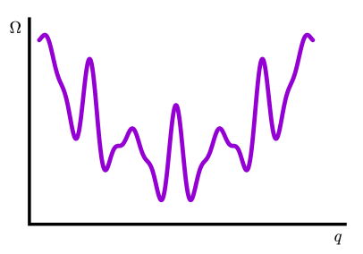
(a)   Without field

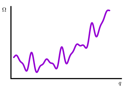
(b)   With field

Figure 1: Cartoon of the free-energy landscape without (a) and with (b) external field. We name $\Omega$ to the free energy, and use the correlation $q$ (see Section 3.2) as collective coordinate, in order to make the simplest possible representation.

We have chosen spin-glasses to study the effect of adding a field, for a variety of reasons: (i) spin glasses are unique among glass formers in that we know that their glassy dynamics arises from a bona fide phase transition [18, 19, 20]; (ii) numerical simulations of spin-glasses are so simple that special-purpose hardware has been built [21, 22, 23]; (iii) high experimental accuracy (thanks to the SQUID) has given experimental access to non-linear susceptibilities long time ago [18] (the equivalent studies in supercooled liquids such as glycerol are only incipient nowadays [24]) and (iv) we understand better than in any other glassy model-system how macroscopic responses relate with microscopic correlation functions that we can compute in the simulations [15, 25].

The layout of the remaining part of this paper is organized as follows. In Section 2 we introduce the model we study and the corresponding observables, before explaining our methods in Section 3. In particular, we explain the protocol in Section 3.1, while the quantities used to compute $\tau$ in Section 3.2. In Section 4 we show the results and the relation between $\tau$ and the field $\varepsilon$ Section 4.2. We explain some effects that virtual states might produce in Section 4.3. Finally, our conclusions are given in Section 5. A contains technical details.

2 Model and observables

We consider the Edwards-Anderson model [26, 27] on a cubic lattice with periodic boundary conditions. The Hamiltonian is

$$\mathcal{H}=-\sum_{\langle i,j\rangle}J_{ij}\sigma_{i}\sigma_{j}\ ,$$ (2)

where $\langle i,j\rangle$ is a sum over lattice nearest-neighbours, $J_{ij}$ is the coupling constant for the bond joining lattice-nodes $i$ and $j$, and $\sigma_{i}=\pm 1$ is the spin at the $i$-th node of the lattice. We set independently for each lattice bond $J_{ij}=\pm 1$ with 50% probability. Let us remark that the $\{J_{ij}\}$ are static variables (quenched disorder), while the $\{\sigma_{i}\}$ are dynamic. Hence, one should perform first the dynamic averaging for a fixed set of couplings (denoted $\langle\ldots\rangle$ hereafter). The averaging over the coupling values is only performed afterwards.

It is well known that model (2) is endowed with a $Z_{2}$ gauge-invariance [28]: $\mathcal{H}$ remains unchanged after the transformation $\sigma_{i}\rightarrow\eta_{i}\sigma_{i},\ J_{ij}\rightarrow\eta_{i}J_{ij}\eta_{j}$ (where $\eta_{i}=\pm 1$ is set independently for each lattice site). Furthermore, the probability for the original couplings $\{J_{ij}\}$ is identical to the probability of their gauge-transform $\{\eta_{i}J_{ij}\eta_{j}\}$. Therefore, meaningful observables should be gauge-invariant as well. In particular, the building block for our observables will be the two-times overlap that compares the value of the very same spin at times $t_{1}$ and $t_{2}$:

$$q_{i}(t_{1},t_{2})=\sigma_{i}(t_{1})\sigma_{i}(t_{2})\,.$$ (3)

[to lighten the notation, we shall omit the argument $(t_{1},t_{2})$ whenever it will be possible; see Section 3.2 for a discussion of the limit $t_{1}-t_{2}\rightarrow\infty$].

In addition, we have introduced a external field which tries to drive away the system from an already-equilibrated initial configuration, thus accelerating the relaxation process. For this, we added to the Hamiltonian (2) a repulsion term

$$\mathcal{H}=-\sum_{\langle i,j\rangle}J_{ij}\sigma_{i}\sigma_{j}\ +\ \varepsilon\sum_{i}\sigma_{i}(t=0)\sigma_{i}(t)\,,$$ (4)

where $\varepsilon$ term can be regarded as a locally varying external magnetic field $h_{i}\equiv\varepsilon\sigma_{i}(t=0)$. Of course, the larger $\varepsilon$, the stronger becomes the repulsion from the (equilibrium) starting condition.

3 Methods

Let us recapitulate two problems that we need to address.

First, as it is clear from (4), we need to reach thermal equilibrium at a low temperature, deep in the glassy phase. We shall solve this problem using a Parallel Tempering algorithm. Unfortunately, the computational resources needed to equilibrate the system grow very fast with the lattice size $L$ [29, 30]. This difficulty, together with the need of studying a large number of samples, has convinced us to restrict ourselves to $L=8$ in this exploratory study.

Second, we need to simulate the $\varepsilon$-dependent Metropolis dynamics at fixed temperatures from those starting configurations. Because this Nature-imitating dynamics should be followed for very long times (for small values of $\varepsilon$, at least), we have found it convenient to use properly adapted multispin coding techniques.

Section 3.1 explains our solutions to both problems (more details can be found in A). The observables that we considered are addressed in Section 3.2.

3.1 Simulations Protocol

We have divided the simulation process in three parts:

Thermalization process.

We need to equilibrate a large number of samples at a low temperature. We have chosen as working temperature $T=0.698\approx 0.63T_{\mathrm{c}}$ (recall that $T_{\mathrm{c}}=1.1019(29)$ is the critical temperature separating the paramagnetic from the spin-glass phase [31]). We have reached equilibrium at $T=0.698$, through a Parallel Tempering simulation, for 1280 samples.

Specifically, our Parallel Tempering simulation for each sample contains 13 clones evenly distributed in the temperature interval $\left[0.698,1.575\right]$. For every clone, we performed 10 Metropolis full-lattice sweeps at fixed temperature. After that, we performed a temperature-swap attempt. We took a total of $2.5\times 10^{8}$ Metropolis sweeps per clone (this simulation time is longer by a factor of $5\times 10^{4}$ than the longest temperature-mixing time identified in Ref. [30] for $L=8$). Once the Parallel Tempering simulation was completed, we took as initial configuration for the next step in our protocol the temperature-clone that occupied the lowest temperature (namely $T=0.698\approx 0.63T_{\mathrm{c}}$).

In practice, we grouped our 1280 samples in 10 bunches of 128 samples each. The 128 samples in a bunch were simulated in parallel using a standard multi-sample multispin coding [32]. Indeed, we coded on a single 128-bits computer word the spins that occupied the very same lattice site for each of the 128 samples in a bunch. As it is usual in multi-sample multispin coding, during the Metropolis part of the simulation we used only one random number per computer word. On the other hand, for the temperature-swap attempt we employed, of course, 128 independent random-numbers for the 128 samples in a bunch.

Overcoming possible correlations.

After the Parallel Tempering, we can assume that the temperature-clone at the lowest temperature for each of our $1280$ samples has been randomly extracted from our target distribution:

$$P(\left\{\sigma_{i}\right\})=P(\left\{J_{ij}\right\})P_{B}(\left\{\sigma_{i}\right\}|\left\{J_{ij}\right\})\,,$$ (5)

where $P(\left\{J_{ij}\right\})$ is the uniform distribution for the coupling constants, while $P_{B}(\left\{\sigma_{i}\right\}|\left\{J_{ij}\right\})$ is the conditional Boltzmann distribution of the spin configuration given the couplings.

However, we note that the Metropolis part of the Parallel Tempering simulation might induce some correlation among the 128 samples in a bunch, due to the sharing of random numbers. In order to alleviate this problem, we have further simulated the temperature clone at the lowest temperature, $T=0.698$, for some additional $2\times 10^{10}$ Metropolis steps. At such a low temperature, we can use an independent random-number for every bit in our computer word with almost no computational overhead [33] (see also A).

After this de-correlating step, we finally have a starting configuration $\{\sigma_{i}(t=0)\}$ for each of our 1280 (statistically independent) samples.

Dynamics with and without field.

Finally, for every value of $\varepsilon$, recall Equation (4), and from every one of our 1280 starting configurations, we simulated $49$ independent trajectories (or replicas). The rationale for such a large number of trajectories per starting point is explained in Section 3.2. We performed Metropolis dynamics at $T=0.698$. Details on our choice of Metropolis dynamics and our multispin coding algorithm can be found in A. The parameters characterizing these simulations are summarized in Table 1.

$\varepsilon$	0	0.0005	0.001	0.003	0.006	0.01	0.02
Metropolis sweeps ($\times 10^{8}$)	200	140	100	26	3.2	0.2	0.16

Table 1: For each of our 1280 samples, and for every value of $\varepsilon$ [recall Equation (4)], we give the total number of Metropolis sweeps that we took along every one of our 49 trajectories. All 49 trajectories started from the same, already equilibrated, starting configuration $\{\sigma_{i}(t=0)\}$ (see Section 3.1). We sampled the state $\{\sigma_{i}(t)\}$, and computed the corresponding observables, 400000 times for each trajectory. The sampling times were evenly distributed along the duration of the run.

3.2 Observables

Our main goal is computing the time scale $\tau^{(\varepsilon)}$, recall Equation (1), in a meaningful way. As we will show below by example, we will be hampered by severe statistical fluctuations (of several types). We shall explain these difficulties and our solutions to overcome them.

Our basic quantity: the time correlation (also known as overlap).

Given the sluggish dynamics in a glassy phase, it is likely that if we observe an spin now, and we look at it again some time later, there is a sizeable probability that the spin remains in the same state [26]. This effect is quantified by the time correlation function, recall Equation (3), with the (already in equilibrium) initial configuration

$$q(t)=\frac{1}{N}\sum_{i}\sigma_{i}(t=0)\sigma_{i}(t)\,,$$ (6)

where $N=8^{3}$ is the total number of spins in our system. Note that the maximum value for the overlap is $q(t)=1$ (i.e. no spin has changed), while the minimum value is $q(t)=-1$ (i.e. every spin has changed).

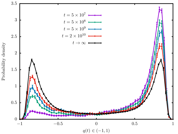
Figure 2: Probability density of the correlation $q(t)$, see Equation (6), as computed at different times for $\varepsilon=0$ over our 1280 samples and starting points. In the limit $t\to\infty$, the configurations $\{\sigma_{i}(t)\}$ and $\{\sigma_{i}(t=0)\}$ becomes statistically independent and the distribution becomes symmetric $P[q(t\to\infty)]=P[-q(t\to\infty)]$, thus reflecting the symmetry of the Hamiltonian in Equation (4) when $\varepsilon=0$. Indeed, as the time proceeds, the asymmetry in the probability density $P[q(t)]$ decreases. The limit $t\to\infty$ was obtained through Parallel Tempering (we equilibrated 8 independent replicas and computed the resulting 28 overlaps, for each of our 1280 samples).

The probability distribution of $q(t)$, $P[q(t)]$, as computed over our 1280 samples for $\varepsilon=0$, unveils extremely slow relaxations and exposes large statistical fluctuations, see Figure 2.

As for the slow dynamics, let at recall that at infinite time $P[q(t)]$ is symmetric $P[q]=P[-q]$ due to the global spin-flip symmetry at $\varepsilon=0$. Nevertheless, see Figure 2, for small $t$ the distribution is strongly peaked at the Edwards-Anderson parameter for $T=0.698$ and system size $L=8$, namely $q_{\mathrm{EA}}\approx 0.844$. As time goes by, $P[q(t)]$ develops a secondary peak at $q(t)=-q_{\mathrm{EA}}$. This secondary peak grows with time. However, even after $2\times 10^{10}$ Metropolis sweeps, we still have $P[q(t)=-q_{\mathrm{EA}}]\approx 0.6P[q(t)=+q_{\mathrm{EA}}]$. This result implies [34] that the time necessary to reach thermal equilibrium with a Metropolis dynamics at $T=0.698$ is enormously longer than $2\times 10^{10}$ full-lattice sweeps. As we anticipated in the Introduction, equilibrating this system at such a low temperature is feasible nowadays only with a non-physical Monte Carlo dynamics, such as Parallel Tempering.

Besides, we observe in Figure 2 that even at very short times there is a sizeable probability of finding any value of $q(t)$. These large fluctuations make unpractical the straightforward definition of the relaxation time $\tau$

$$q(t=\tau)=0\,.$$ (7)

In order to overcome this problem, we shall need to consider statistical fluctuations in greater details.

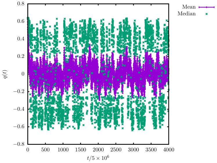
Figure 3: Time evolution of the median and the mean of the conditional probability distribution function $P[q(t)\,|\,\{J_{ij},\sigma_{i}(t=0)\}]$, defined in Equation (8), as computed from the 49 replicas for our sample #107 at $\varepsilon=0$. We show errorbars for the mean. Errorbars for the median are as large as the median itself (indeed, the median is ill-defined for probability density functions with two bands, each of them with the same weight).

Fluctuations within the same sample and starting point.

A spin-glass practitioner will surely expect large statistical fluctuations among different samples (recall that a sample is characterized by a set of coupling constants $\{J_{ij}\}$). Probably, large fluctuations would also be expected if different starting points $\{\sigma_{i}(t=0)\}$ are compared for a given sample. What it is more worrisome is that we did find large statistical fluctuations for a given sample and starting point $\{J_{ij},\sigma_{i}(t=0)\}$, see Figure 3. Unfortunately, this means that, in order to characterize the conditional probability

$$P[q(t)\,|\,\{J_{ij},\sigma_{i}(t=0)\}]$$ (8)

one needs to consider a large number of trajectories, all of them sharing the same starting configuration. Given our computational resources, we had to restrict ourselves to 49 independent trajectories per $\{J_{ij},\sigma_{i}(t=0)\}$. By analogy with the problem of particle diffusion, one could think that the ensemble of these 49 trajectories encode the solution of the Fokker-Planck equation (rather than the Langevin dynamics) for the conditional probability in Equation (8).

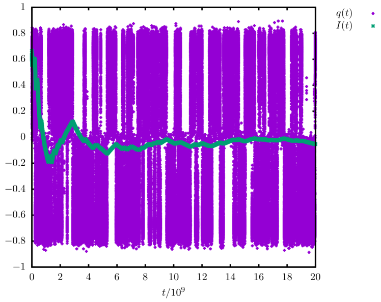
Figure 4: Comparison of the time evolution $I(t)$ (green), recall Equation (9), and $q(t)$ (purple), as computed for a randomly chosen sample for $\varepsilon=0$, from just one replica. We do not average over the 49 available replicas, in order to show that $I(t)$ displays a much softer time evolution.

The large fluctuations of the conditional probability $P[q(t)\,|\,\{J_{ij},\sigma_{i}(t=0)\}]$ is evinced in Figure 3 by the fact that the median and mean of the distribution are wildly different. Furthermore, for this particular sample, the median is ill-defined as the $P[q(t)\,|\,\{J_{ij},\sigma_{i}(t=0)\}]$ is bimodal and gapped. We thus need to further refine our dynamical study.

Smoothing $q(t)$ by time averaging.

Clearly, we need to build from $q(t)$ a new observable, with less fluctuations. To that end in mind, we considered the time average

$$I(t)\equiv\frac{\displaystyle\sum_{t^{\prime}\leq t}\langle q_{t^{\prime}}\rangle_{r}}{\displaystyle\sum_{t^{\prime}\leq t}1}\simeq\frac{1}{t}\int_{0}^{t}\langle q(t^{\prime})\rangle_{r}dt^{\prime}\,,$$ (9)

where now $\langle\ \rangle_{r}$ is the average over the 49 replicas, which reduces the fluctuations.

In Figure 4, we compare $I(t)$ and $q(t)$, as computed for a randomly chosen sample (in order to emphasize their different behavior, $I(t)$ and $q(t)$ where computed from the very same single replica in Figure 4). We see that $I(t)$ shows a softer time evolution. Furthermore, we see that short but inconsequential excursions to distant states [which results in $q(t)<0$ for very short time intervals] have a smaller impact on $I(t)$.

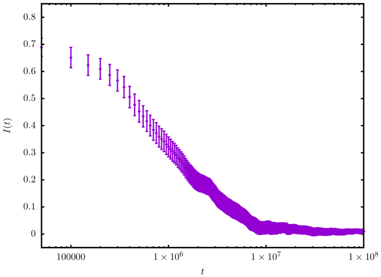
Figure 5: The time evolution of the time-average $I(t)$, as computed for our sample #50 at $\varepsilon=0$, is shown with its statistical error. Even though (in the limit of an infinite number of replicas) $I(t)$ should be positive for all times, our 49-replicas estimate becomes negative at finite $t$. Therefore, estimating the relaxation time by requiring $I(t=\tau)=0$ would be a meaningless choice. In fact, $I(t=\tau)=0$ actually indicates the time when our signal-to-noise ratio becomes of order one.

Now, we need to find a reasonable way to extract the relaxation time $\tau$ from $I(t)$. One obvious solution is to require $I(t=\tau)=a$, for some suitable value $a$. In order to chose $a$, we need some reflection. On the one hand, $a$ should be significantly smaller than $1$, to ensure that the system has escaped from the valley around its starting configuration. On the other hand, a too small $a$ would result in large errors. In fact, we expect for the replica-average of $q(t)$

$$\langle q(t)\rangle_{r}=\sum_{n=2}^{2^{N}}a_{n}e^{-t/\tau_{n}}\,,$$ (10)

which, when substituted in the integral form of (9), gives us

$$I(t)=\frac{1}{t}\sum_{n=2}^{2^{N}}a_{n}\tau_{n}\left[1-e^{-t/\tau_{n}}\right]\,.$$ (11)

Now, because we expect that $a_{n},\,\tau_{n}>0$, then

$$I(t\rightarrow 0) = \sum_{n}a_{n}=1\,,$$ (12)

$$I(t\rightarrow\infty) = \frac{1}{t}\sum_{n}a_{n}\tau_{n}=0\,,$$ (13)

in other words, $I(t)$ which does not vanish at any finite time. For this reason, taking $a=0$, as (7) might suggest, would implies that our statistical errors would equal (in order of magnitude) the value of $I(t)$ itself. So we have to take a value of $a$ far from $0$ which guarantees that the statistical errors do not spoil our results, see Figure 5.

In order to make a reasonable choice for $a$, we consider a toy model for $\langle q(t)\rangle_{r}$, with only two autocorrelation times

$$\langle q(t)\rangle_{r}^{\mathrm{toy}}=(1-q_{\mathrm{EA}})\,\mathrm{e}^{-t/\tau_{\mathrm{fast}}}\ +\ q_{\mathrm{EA}}\,\mathrm{e}^{-t/\tau_{\mathrm{slow}}}\,.$$ (14)

If we now take the limit $\tau_{\mathrm{fast}}/\tau_{\mathrm{slow}}\to 0$, and recall $q_{\mathrm{EA}}\approx 0.844$, we immediately find that requiring $I(t=\tau)=a$, with $a=0.437$ results in $\tau=1.5\tau_{slow}$, which is a fairly sensible estimate of the relaxation time. Furthermore, Figure 5 tells us that $a=0.437$ is sufficiently far away from zero to allow for a safe determination of $\tau$, given the size of our statistical errors.

4 Results and discussion

4.1 On the computation of characteristic times for each sample

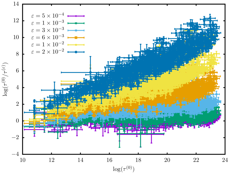
Figure 6: $\log(\tau^{(0)}/\tau^{(\varepsilon)})$ vs $\log(\tau^{(0)})$ for the different values of $\varepsilon$, as computed for all the pairs of samples and initial configurations that allowed us to estimate statistical errors through the Boostrap method explained in Section 4 (we were able to compute errors for about 65% of our 1280 samples).

As we explained above, we compute a characteristic time scale $\tau^{(\varepsilon)}$ through the relation

$$I(\tau^{(\varepsilon)})=0.437\,.$$ (15)

Note that every sample and starting configuration $\{J_{ij},\sigma_{i}(t=0)\}$ has its own $\tau^{(\varepsilon)}$ for every value of the external field $\varepsilon$. Now, it turns out that the order of magnitude of $\tau^{(\varepsilon)}$ fluctuates heavily among the different $\{J_{ij},\sigma_{i}(t=0)\}$ (see Figure 6). Therefore, in order to properly quantify the field-effect, we shall compute $\log[\tau^{(0)}/\tau^{(\varepsilon)}]$ for every pair $\{J_{ij},\sigma_{i}(t=0)\}$.

The main problems that we have needed to address upon computing $\log[\tau^{(0)}/\tau^{(\varepsilon)}]$ have been the following:

1. For approximately a 35% of pairs $\{J_{ij},\sigma_{i}(t=0)\}$, the condition (15) is not met for $\varepsilon=0$. This is hardly surprising, on the view of the sluggish dynamics illustrated in Figure 2. The same problem has occasionally arisen for $\varepsilon>0$, although to a lesser degree.

2. We need to estimate errorbars for both $\log\tau^{(0)}$ and $\log[\tau^{(0)}/\tau^{(\varepsilon)}]$.

To address the first problem, we have simply discarded from our analysis all pairs $\{J_{ij},\sigma_{i}(t=0)\}$ for wich we could not compute reliably either $\tau^{(0)}$ or $\tau^{(\varepsilon)}$. Reliable here does not only mean that condition (15) was met, but we also require that errorbars could be computed (see below). Essentially, this amounts to say that we are computing conditional probabilities over the pairs $\{J_{ij},\sigma_{i}(t=0)\}$, the imposed condition being $\tau^{(0)}<2\times 10^{10}$.

In order to compute errorbars for $\log\tau^{(0)}$ and $\log[\tau^{(0)}/\tau^{(\varepsilon)}]$, we have employed a Bootstrap method [35]. Specifically, we have generated 1000 resampled populations. Each resampled population is obtained by choosing randomly, with uniform probability, 49 trajectories out of our set of 49 trajectories (the same trajectory could be chosen several times, of course). Then, by averaging over the 49 trajectories in the resampled population, we recomputed $\langle q(t)\rangle_{r}$ and $I(t)$, and obtained the corresponding $\log\tau^{(0)}$ and $\log[\tau^{(0)}/\tau^{(\varepsilon)}]$. Now, we encountered one of three alternatives:

• If we were able to compute $\log\tau^{(0)}$ and $\log[\tau^{(0)}/\tau^{(\varepsilon)}]$ for every one of the 1000 resampled populations, then we assigned to that pair $\{J_{ij},\sigma_{i}(t=0)\}$ the values of $\log\tau^{(0)}$ and $\log[\tau^{(0)}/\tau^{(\varepsilon)}]$ obtained by averaging over the original set of 49 trajectories. Errors were computed by using standard Boostrap formulae.

• If we were able to compute both $\log\tau^{(0)}$ and $\log[\tau^{(0)}/\tau^{(\varepsilon)}]$ for at least 84% of the 1000 resampled populations, then we assigned to that pair $\{J_{ij},\sigma_{i}(t=0)\}$ the median values of $\log\tau^{(0)}$ and $\log[\tau^{(0)}/\tau^{(\varepsilon)}]$. Errors were computed as the halved difference between percentiles 84 and 16.

• We discarded pairs $\{J_{ij},\sigma_{i}(t=0)\}$ that did not fall in any of the two cases above.

The above analysis program produced values of $\log\tau^{(0)}$ and $\log[\tau^{(0)}/\tau^{(\varepsilon)}]$, see Figure 6, for 65% of the pairs $\{J_{ij},\sigma_{i}(t=0)\}$. The detailed analysis of the $\varepsilon$-dependence will be addressed next.

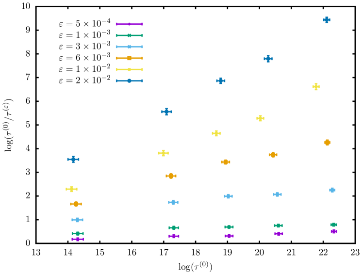
Figure 7: The noise for $\log(\tau^{(0)}/\tau^{(\varepsilon)})$ and $\log(\tau^{(0)})$ is considerably reduced, as compared to Figure 6, by grouping the pairs of samples and starting configurations in quintiles (see Section 4.2 for details). The quintiles procedure does not arise the correlation between $\log(\tau^{(0)})$ and the response to the extenal field.

4.2 On the relation between $\tau^{(\varepsilon)}$ and $\varepsilon$

In spite of the strong fluctuations, we note an important feature in Figure 6. Pairs $\{J_{ij},\sigma_{i}(t=0)\}$ with a large $\log\tau^{(0)}$ are prone to a stronger reaction to $\varepsilon$. In terms of the cartoon in Figure 1, one would say that the larger the barrier, the stronger the field-effect. This suggest already a violation of the linear relationship between $\varepsilon$ and $\log\tau^{(\varepsilon)}$ suggested in Equation (1). We shall further elaborate on non-linearities in Section 4.3.

In order to reduce the noise, while still respecting the strong correlation between $\log\tau^{(0)}$ and the response to the field, we have organized our pairs $\{J_{ij},\sigma_{i}(t=0)\}$ in quintiles according to their $\log\tau^{(0)}$ value. Specifically, for every value of $\varepsilon$, we have sorted our data according to $\log\tau^{(0)}$. Next, we have grouped them in five sets of pairs with the same number of elements. Obtaining exactly the same number of elements in each group was impossible, because the total number of pairs that met the criteria explained in Section 4.1 was not a multiple of five, but the differences among the cardinalities of the five sets was, at most, of one element. The group containing the pairs $\{J_{ij},\sigma_{i}(t=0)\}$ with the smallest $\log\tau^{(0)}$ is referred to as quintile 1, and so on. Our motivation for chosing quintiles rather than deciles (or even a finer division), was keeping a large enough number of pairs within in each group. The basic quantity that we have computed is the arithmetic mean of both $\log\tau^{(0)}$ and $\log[\tau^{(0)}/\tau^{(\varepsilon)}]$, for all pairs belonging to a given quintile.

In order to estimates errors for the average $\log\tau^{(0)}$ and $\log[\tau^{(0)}/\tau^{(\varepsilon)}]$ of each quintile, we used again a boostrap method. We generated 1000 resampled populations by choosing randomly, with uniform probability, 1280 pairs $\{J_{ij},\sigma_{i}(t=0)\}$ among those in the original population (note that the number of pairs that met the the criteria explained in Section 4.1 varied among different ressampled populations). In order to account as well for our errors in the determination of $\log\tau^{(0)}$ and $\log[\tau^{(0)}/\tau^{(\varepsilon)}]$ (these errors were due to our limited number of trajectories for each pair), we modified the estimates in the original population by adding two random numbers. For each pair, these two random numbers were independent and normal distributed, with zero average and dispersions equal to our errors for $\log\tau^{(0)}$ and $\log[\tau^{(0)}/\tau^{(\varepsilon)}]$, respectively. For every resampled population, we carried out the full quintile procedure explained above. Errors for the average $\log\tau^{(0)}$ and $\log[\tau^{(0)}/\tau^{(\varepsilon)}]$ of each quintile were computed with the standard boostrap formula. The outcome of the quintile procedure is summarized in Figure 7.

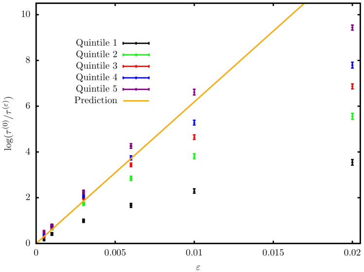
Figure 8: Quintile averaged $\log(\tau^{(0)}/\tau^{(\varepsilon)})$ as a function of the extenally applied field $\varepsilon$ (data were taken from Figure 7). The orange line is given by Equation (1), where we take $\Delta q=q_{\mathrm{EA}}\approx 0.844$. Recall that $q_{\mathrm{EA}}$ is the position of the maximum of the probability density shown in Figure 2.

Next, we consider the quintile-average of $\log(\tau^{(0)}/\tau^{(\varepsilon)})$ as a function the externally applied field, see Figure 8. We note the following features:

• For all five quintiles, and for small-enough fields, we can identify in Figure 8 a linear relationship between $\varepsilon$ and $\log\tau^{(\varepsilon)}$. Furthermore, the slopes close to $\varepsilon=0$ approach the predicted one (orange line in Figure 8). Nevertheless, the region of validity of the linear approximation is strongly quintile-dependent. In particular, for the slowest pairs $\{J_{ij},\sigma_{i}(t=0)\}$, the region where the linear approximation is reasonable extends up to $\varepsilon\approx 0.01$. This implies that we could have guessed the behavior for smaller $\varepsilon$ with far lesser numerical effort.

• In addition, the slowest pairs $\{J_{ij},\sigma_{i}(t=0)\}$ show a reduction of three orders of magnitude in their relaxation time for $\varepsilon$ near $0.01$. Notice that, at $\varepsilon=0$, the fastest pairs are thousand times faster than the slowest pairs. Therefore, the external field produces an homogenization of the relaxation times (homogenization in order of magnitude, at least).

• However, we note that for some quintiles the external field increases $\log(\tau^{(0)}/\tau^{(\varepsilon)})$ above the prediction by the linear approximation, see the orange line in Figure 8. Clearly, some unsuspected processes enlarge the ability of the field to reduce the relaxation times. We speculate in Section 4.3 about one such escaping mechanism.

4.3 Virtual states

We discuss here how virtual states might produce an enhanced scape rate from the starting configuration, in the presence of an external field. In order to do that, we first need to relate the calculation process that we use to estimate $\tau$ with the effective potential.

Consider a sample and a starting configuration at $\varepsilon=0$. Let the time elapsed from system prepation go to infinity, so that all statistical correlations between the initial and the current configuration fade away. Under such circumstances, the probability density $P(q)$ for the overlap $q$ between the starting and the current configuration defines the effective potential $\Omega(q)$ through

$$P(q)\propto e^{-N\Omega(q)}\,,$$ (16)

(the normalization is not relevant now). Keep in mind that $\Omega(q)$ depends not only on the sample, but on the starting configuration as well (in fact, $\Omega(q)$ can be regarded as the Franz-Parisi potential [36]). For the purpose of discussion, let us consider an effective-potential profile like the one in Figure 9, where we plot the derivative of the effective potential as a function of the correlation. If we maximize the probability given by equation (16), we find that the equilibrium states satisfy $\Omega^{\prime}(q)=0$ and $\Omega^{\prime\prime}(q)>0$, so we have two symmetric real states at $q\approx\pm q_{\mathrm{EA}}$, separated by a saddle-point at $q=0$.

Figure 9: Schematic representation of the derivative of the Franz-Parisi-like potential in Equation (16). Stationary points are given by the condition $\Omega^{\prime}(q)=-\varepsilon$ (recall that $\varepsilon$ is a repulsion). Local minima verify in addition that $\Omega^{\prime\prime}(q)>0$. At $\varepsilon=0$ we encounter two local minima separated by a saddle point at $q=0$. Instead, at $\varepsilon>0$ we find three local minima separated by two saddle points. The arrow indicates a characteristic value of $q$, employed in the computation of $\tau$ (see text).

Now, our procedure for computing $\tau$ declares that the system has escaped from the initial valley at $q\approx q_{\mathrm{EA}}$ when the overlap $q(t)$ goes below some threshold, indicated by an arrow in Figure 9. In fact, we know that the system will be tethered to $q\approx q_{\mathrm{EA}}$ until a random excursion will take it to the saddle-point at $q=0$. Once the saddle-point is reached, the transit to the minimum at $q\approx-q_{\mathrm{EA}}$ is very fast. Therefore, the logarithm of $\tau^{(\varepsilon=0)}$ is given by the barrier ($B$), namely by the area between the $q$ axis and the function $\Omega^{\prime}(q)$ (filled area in Figure 9).

In the presence of an external field, the local minima are given by the conditions $\Omega^{\prime}(q)=-\varepsilon$ and $\Omega^{\prime\prime}(q)>0$. Therefore, the two original minima at $q\approx\pm q_{\mathrm{EA}}$ get small corrections of order $\varepsilon$. It is more significant, however, that new states can appear for $\varepsilon>0$, such as the one depicted in the figure. We name this new minimum a virtual state. Now, if the arrow in Figure 9 lies to the right of the virtual state, the most probable process for escaping the original minimum at $q\approx q_{\mathrm{EA}}$ is not jumping to the symmetric state at $q\approx-q_{\mathrm{EA}}$, but stopping at the virtual state. The corresponding barrier is given by the area of the right pink region in Figure 9. Instead, the relevant barrier for the escape process to $q\approx-q_{\mathrm{EA}}$ (which is the only escape path at $\varepsilon=0$) is given by the area of the two pink regions in the figure. In other words, $\log\tau^{(\varepsilon)}$ will be quite smaller than what one would have guessed from $\log\tau^{(\varepsilon=0)}$.

In order to give some flesh to the virtual-state idea, we show in Figure 10 the probability density of $q(t)$, conditional to $q(t)>0$ for one particular sample and starting configuration, chosen because of its anomalously large ratio $\log\tau^{(\varepsilon=5\times 10^{-4})}/\log\tau^{(0)}$. At $\varepsilon=0$ we observe two well defined states (i.e. local maxima of the probability density) at $q\approx 0.84$ and $q\approx 0.6$. When $\varepsilon$ increases, a new local maximum (a virtual state?) emerges at $q\approx 0.1$.

Figure 10: Semilogarithmic plot of the probability density conditional to $q(t)>0$, for a sample and starting configuration remarkable for its large value of $\log\tau^{(\varepsilon=5\times 10^{-4})}/\log\tau^{(0)}$. We first computed the conditional probability density for each replica, and only afterwards averaged over the 49 trajectories. Besides the local maxima at $q\approx 0.84$ and $q\approx 0.6$, which are almost unaffected by the external field, a new state (a virtual state, probably) emerges at $q=0.1$ upon increasing $\varepsilon$.

5 Conclusion

The huge relaxation times of glasses make challenging their study. This difficulty has prompted researchers to invent non-physical dynamics, correctly sampling the Boltzmann weight even at low temperatures (see e.g. Refs. [7, 8, 4, 5, 6]). However, reaching equilibrium is only half of the problem when (as it is the case for many glass formers), the glass transition is not accompanied by significant changes in static quantities, think for instance of structure factors or density profiles. Under such circumstances, one is forced to study Nature-imitating dynamics starting from equilibrium configurations. Dynamics of this kind are extremely slow.

A method to reduce free-energy barriers, hence accelerating relaxations, consists in placing the system in an external field. This idea has been used experimentally to extract the spin-glass correlation length [13, 14] by placing the spin-glass in an external magnetic field. Similar studies are being conducted for the dielectric response of glass-forming liquids [16, 17]. Here, we perform a preliminary exploration of this strategy in the highly controlled context of the simulation of a small spin-glass system in three dimensions. Let us recall that our external field $\varepsilon$ should be proportional to the square of the external fields used in experiments.

Our simulations have shown that the external field indeed reduces the relaxation times, which can be regarded as a reduction of the height of the effective barriers (recall the cartoon in Figure 1). Nevertheless, we have found rather dramatic statistical fluctuations. We have needed to resort to robust statistical methods (i.e. studying quintiles), in order to control these fluctuations. After taking care of fluctuations, we have found that our naive expectation of a linear dependence on the external field of the logarithm of the relaxation time is only full-filed for very small fields.

When regarded as a purely numerical strategy, we have found that the external field may reduce the relaxation times by some three orders of magnitude. Furthermore, the field strongly enhances the homogeneity of the relaxation times of the different samples and starting configurations.

Finally, we have discussed a possible mechanism (namely the formation of a virtual state), to explain the extreme sensitivity to the external field of some samples and starting configurations.

Appendix A Multispin coding at fixed temperatures

Our multisample multispin coding Parallel Tempering simulation is fully standard and does not deserve any special comment. However, we have found it useful to describe here our simulation methods at fixed temperature in the presence of the external field, where random numbers are not recycled in the simulation of the different bits in a computer word.

As usual in multispin coding simulations, the key of our program is that we can use a binary representation of $J_{ij}$ and $\sigma_{i}$, namely $J_{ij}=\left\{-1,1\right\}\rightarrow b^{J}_{ij}=\left\{1,0\right\}$ and $\sigma_{i}=\left\{-1,1\right\}\rightarrow b^{\sigma}_{i}=\left\{0,1\right\}$. Multiplications of spin variables, for instance, are equivalent to the XOR boolean operation. Furthermore, we exploit that boolean operations (such as AND, OR, XOR, NOT,…) are carried out in parallel for all bits in a computer word.

We employ a modified version of the Metropolis algorithm for a spin-system in a field, which is particularly well suited for multi-spin coding simulations. Let us attempt to flip a spin, the corresponding energy change is composed of two terms, $\Delta E=\Delta E_{J}+\Delta E_{\varepsilon}$. The first term $\Delta E_{J}\in\{0,\pm 4,\pm 8,\pm 12\}$ is the energy change due to the exchange term in the Hamiltonian in Equation (4). On the other hand, $\Delta E_{\varepsilon}=-2\varepsilon\sigma_{i}(t)\sigma_{i}(t=0)$ is the energy change due to the external field. Hence, the spin flip is accepted with a probability which is a product of two terms

$$\mathrm{Prob[spin\ flip]}=\min\left\{1,\exp(-\Delta E_{J}/T)\right\}\,\cdot\min\left\{1,\exp(-\Delta E_{\varepsilon}/T)\right\}\,.$$ (17)

In practice, the Monte Carlo dynamics is implemented as

$$b^{\sigma}_{i}(t+1) = b_{i}^{(\mathrm{change})}\,\mathrm{XOR}\,b^{\sigma}_{i}(t)\,,$$ (18)

$$b_{i}^{(\mathrm{change})} = b_{i}^{(\mathrm{change},J)}\,\mathrm{AND}\,b_{i}^{(\mathrm{change},\varepsilon)}\,,$$ (19)

with

$$\mathrm{Probability}\Big{[}b_{i}^{(\mathrm{change},J)}=1\Big{]} = \min\left\{1,\exp(-\Delta E_{J}/T)\right\}\,,$$ (20)

$$\mathrm{Probability}\Big{[}b_{i}^{(\mathrm{change},\varepsilon)}=1\Big{]} = \min\left\{1,\exp(-\Delta E_{\varepsilon}/T)\right\}\,.$$ (21)

In order to avoid unwanted correlations, the 256 bits used to update a computer word, namely 128 bits $b_{i}^{(\mathrm{change},J)}$ and 128 bits $b_{i}^{(\mathrm{change},\varepsilon)}$, should be statistically independent. A naive implementation of the method would require getting 256 independent random numbers per computer word, which is rather costly. Fortunately, there is a better way.

For the obtention of the bits $b_{i}^{(\mathrm{change},J)}$, we employ the Daemons algorithm by Ito and Kanada [37] which, up to our knowledge, needs a smaller number of Boolean operations than any other method. As for the random numbers, we observe that the smallest exchange-energy barrier to be overcome, namely $\Delta E_{J}=4$, is rather large as compared to our working temperature $T=0.698$. Hence, only very rarely the thermal bath allows us to overcome any energy barrier, and a Gillespie-Bortz method is called for [38, 39].

For the sake of completeness, let us recall how we use the Gillespie-Bortz method to run our Monte Carlo algorithm for long times without the need to generate a large number of random numbers. Indeed, in a naif simulation, one would draw for each bit an independent, uniformly distributed random number $0<R<1$. The corresponding bit is set to 1 only if $R<p$, where $p$ is some probability. The crucial observation is that, if $p$ is small enough (in our case $p\leq\mathrm{e}^{-4/T}=0.0032\ldots$), almost every bit will be zero with very few exceptions. The Gillespie-Bortz method allows to correctly select those exceptions, with very little effort. Let us imagine that we have just set the bit to one, the probability that the next bit set to one will be found after $k$ independent extractions of the random numbers $R$ is $(1-p)^{k-1}p$. What we do is to extract $k$ according to that probability. Indeed, the typical value of $k$ is $1/p$. So, in our case, we can obtain approximately 308 random bits from a single extraction of $k$. For more details about the implementation of these ideas, the reader may wish to check Ref. [33].

As for the bits $b_{i}^{(\mathrm{change},\varepsilon)}$, the straigtforward implementation is

$$b_{i}^{(\mathrm{change},\varepsilon)}=\Big{[}\,\mathrm{NOT}[\,b_{i}^{(0)}\,\mathrm{XOR}\,b_{i}^{(t)}\,]\,\Big{]}\ \mathrm{OR}\ [R<\exp(-2\varepsilon/T)]\,,$$ (22)

where $0<R<1$ is an uniformly distributed random number, and the corresponding bit is set to one if the inequality is fulfilled. However, the probability $\exp(-2\varepsilon/T)$ is close to 1, due to the smallness of $\varepsilon$, which would preclude us from using Gillespie methods. Fortunately, the problem is fairly easy to fix:

$$b_{i}^{(\mathrm{change},\varepsilon)}=$$ (23)

$$\Big{[}\,\mathrm{NOT}[\,b_{i}^{(0)}\,\mathrm{XOR}\,b_{i}^{(t)}\,]\,\Big{]}\ \mathrm{OR}\ \ \Big{[}\,\mathrm{NOT}\,[\,R<(1-\exp(-2\varepsilon/T))\,]\,\Big{]} \,.$$

References

References

- [1] Ludovic Berthier and Giulio Biroli. Theoretical perspective on the glass transition and amorphous materials. Rev. Mod. Phys., 83:587–645, Jun 2011.
- [2] Andrea Cavagna. Supercooled liquids for pedestrians. Physics Reports, 476(4):51–124, 2009.
- [3] Robert H. Swendsen and Jian-Sheng Wang. Nonuniversal critical dynamics in monte carlo simulations. Phys. Rev. Lett., 58:86–88, Jan 1987.
- [4] Tomás S. Grigera and Giorgio Parisi. Fast Monte Carlo algorithm for supercooled soft spheres. Phys. Rev. E, 63:045102, Mar 2001.
- [5] L. A. Fernández, V. Martín-Mayor, and P. Verrocchio. Critical behavior of the specific heat in glass formers. Phys. Rev. E, 73:020501, Feb 2006.
- [6] Andrea Ninarello, Ludovic Berthier, and Daniele Coslovich. Models and algorithms for the next generation of glass transition studies. Phys. Rev. X, 7:021039, Jun 2017.
- [7] K. Hukushima and K. Nemoto. Exchange Monte Carlo method and application to spin glass simulations. J. Phys. Soc. Japan, 65:1604, 1996.
- [8] E. Marinari. Optimized Monte Carlo methods. In J. Kerstész and I. Kondor, editors, Advances in Computer Simulation. Springer-Verlag, 1998.
- [9] C. L. E. Struik. Physical Aging in Amorphous Polymers and Other Materials. Elsevier, Amsterdam, 1980.
- [10] E. Vincent, J. Hammann, M. Ocio, J.-P. Bouchaud, and L. F. Cugliandolo. Slow dynamics and aging in spin glasses. In M. Rubí and C. Pérez-Vicente, editors, Complex Behavior of Glassy Systems, number 492 in Lecture Notes in Physics. Springer, 1997.
- [11] M. Mézard, G. Parisi, and M. Virasoro. Spin-Glass Theory and Beyond. World Scientific, Singapore, 1987.
- [12] A. P. Young. Spin Glasses and Random Fields. World Scientific, Singapore, 1998.
- [13] Y. G. Joh, R. Orbach, G. G. Wood, J. Hammann, and E. Vincent. Extraction of the spin glass correlation length. Phys. Rev. Lett., 82:438–441, Jan 1999.
- [14] Samaresh Guchhait and Raymond L. Orbach. Magnetic field dependence of spin glass free energy barriers. Phys. Rev. Lett., 118:157203, Apr 2017.
- [15] M. Baity-Jesi, E. Calore, A. Cruz, L. A. Fernandez, J. M. Gil-Narvion, A. Gordillo-Guerrero, D. Iñiguez, A. Maiorano, E. Marinari, V. Martin-Mayor, J. Monforte-Garcia, A. Muñoz Sudupe, D. Navarro, G. Parisi, S. Perez-Gaviro, F. Ricci-Tersenghi, J. J. Ruiz-Lorenzo, S. F. Schifano, B. Seoane, A. Tarancon, R. Tripiccione, and D. Yllanes. Matching microscopic and macroscopic responses in glasses. Phys. Rev. Lett., 118:157202, Apr 2017.
- [16] D. L’Hôte, R. Tourbot, F. Ladieu, and P. Gadige. Control parameter for the glass transition of glycerol evidenced by the static-field-induced nonlinear response. Phys. Rev. B, 90:104202, Sep 2014.
- [17] F. Ladieu, C. Brun, and D. L’Hôte. Nonlinear dielectric susceptibilities in supercooled liquids: A toy model. Phys. Rev. B, 85:184207, May 2012.
- [18] K. Gunnarsson, P. Svedlindh, P. Nordblad, L. Lundgren, H. Aruga, and A. Ito. Static scaling in a short-range Ising spin glass. Phys. Rev. B, 43:8199–8203, 1991.
- [19] M. Palassini and S. Caracciolo. Universal finite-size scaling functions in the 3D Ising spin glass. Phys. Rev. Lett., 82:5128–5131, 1999.
- [20] H. G. Ballesteros, A. Cruz, L. A. Fernandez, V. Martín-Mayor, J. Pech, J. J. Ruiz-Lorenzo, A. Tarancon, P. Tellez, C. L. Ullod, and C. Ungil. Critical behavior of the three-dimensional Ising spin glass. Phys. Rev. B, 62:14237–14245, 2000.
- [21] A. T. Ogielski. Dynamics of three-dimensional Ising spin glasses in thermal equilibrium. Phys. Rev. B, 32:7384, 1985.
- [22] F. Belletti, M. Cotallo, A. Cruz, L. A. Fernandez, A. Gordillo, A. Maiorano, F. Mantovani, E. Marinari, V. Martín-Mayor, A. Muñoz Sudupe, D. Navarro, S. Perez-Gaviro, J. J. Ruiz-Lorenzo, S. F. Schifano, D. Sciretti, A. Tarancon, R. Tripiccione, and J. L. Velasco. Simulating spin systems on IANUS, an FPGA-based computer. Comp. Phys. Comm., 178:208–216, 2008.
- [23] M. Baity-Jesi, R. A. Baños, Andres Cruz, Luis Antonio Fernandez, Jose Miguel Gil-Narvion, Antonio Gordillo-Guerrero, David Iniguez, Andrea Maiorano, F. Mantovani, Enzo Marinari, Victor Martín-Mayor, Jorge Monforte-Garcia, Antonio Muñoz Sudupe, Denis Navarro, Giorgio Parisi, Sergio Perez-Gaviro, M. Pivanti, F. Ricci-Tersenghi, Juan Jesus Ruiz-Lorenzo, Sebastiano Fabio Schifano, Beatriz Seoane, Alfonso Tarancon, Raffaele Tripiccione, and David Yllanes. Janus II: a new generation application-driven computer for spin-system simulations. Comp. Phys. Comm, 185:550–559, 2014.
- [24] S. Albert, Th. Bauer, M. Michl, G. Biroli, J.-P. Bouchaud, A. Loidl, P. Lunkenheimer, R. Tourbot, C. Wiertel-Gasquet, and F. Ladieu. Fifth-order susceptibility unveils growth of thermodynamic amorphous order in glass-formers. Science, 352(6291):1308–1311, 2016.
- [25] M. Baity-Jesi, E. Calore, A. Cruz, L. A. Fernandez, J. M. Gil-Narvion, A. Gordillo-Guerrero, D. Iñiguez, A. Maiorano, E. Marinari, V. Martin-Mayor, J. Moreno-Gordo, A. Muñoz Sudupe, D. Navarro, G. Parisi, S. Perez-Gaviro, F. Ricci-Tersenghi, J. J. Ruiz-Lorenzo, S. F. Schifano, B. Seoane, A. Tarancon, R. Tripiccione, and D. Yllanes. Aging rate of spin glasses from simulations matches experiments. Phys. Rev. Lett., 120:267203, Jun 2018.
- [26] S. F. Edwards and P. W. Anderson. Theory of spin glasses. Journal of Physics F: Metal Physics, 5:965, 1975.
- [27] S. F. Edwards and P. W. Anderson. Theory of spin glasses. ii. J. Phys. F, 6(10):1927, 1976.
- [28] G. Toulouse. Theory of the frustration effect in spin glasses. Communications on Physics, 2:115, 1977.
- [29] R. Alvarez Baños, A. Cruz, L. A. Fernandez, J. M. Gil-Narvion, A. Gordillo-Guerrero, M. Guidetti, A. Maiorano, F. Mantovani, E. Marinari, V. Martín-Mayor, J. Monforte-Garcia, A. Muñoz Sudupe, D. Navarro, G. Parisi, S. Perez-Gaviro, J. J. Ruiz-Lorenzo, S. F. Schifano, B. Seoane, A. Tarancon, R. Tripiccione, and D. Yllanes. Nature of the spin-glass phase at experimental length scales. J. Stat. Mech., 2010:P06026, 2010.
- [30] A Billoire, L A Fernandez, A Maiorano, E Marinari, V Martin-Mayor, J Moreno-Gordo, G Parisi, F Ricci-Tersenghi, and J J Ruiz-Lorenzo. Dynamic variational study of chaos: spin glasses in three dimensions. Journal of Statistical Mechanics: Theory and Experiment, 2018(3):033302, 2018.
- [31] M. Baity-Jesi, R. A. Baños, Andres Cruz, Luis Antonio Fernandez, Jose Miguel Gil-Narvion, Antonio Gordillo-Guerrero, David Iniguez, Andrea Maiorano, F. Mantovani, Enzo Marinari, Victor Martín-Mayor, Jorge Monforte-Garcia, Antonio Muñoz Sudupe, Denis Navarro, Giorgio Parisi, Sergio Perez-Gaviro, M. Pivanti, F. Ricci-Tersenghi, Juan Jesus Ruiz-Lorenzo, Sebastiano Fabio Schifano, Beatriz Seoane, Alfonso Tarancon, Raffaele Tripiccione, and David Yllanes. Critical parameters of the three-dimensional Ising spin glass. Phys. Rev. B, 88:224416, 2013.
- [32] M. E. J. Newman and G. T. Barkema. Monte Carlo Methods in Statistical Physics. Clarendon Press, Oxford, 1999.
- [33] Luis Antonio Fernández and Víctor Martín-Mayor. Testing statics-dynamics equivalence at the spin-glass transition in three dimensions. Phys. Rev. B, 91:174202, May 2015.
- [34] A. D. Sokal. Monte Carlo methods in statistical mechanics: Foundations and new algorithms. In C. DeWitt-Morette, P. Cartier, and A. Folacci, editors, Functional Integration: Basics and Applications (1996 Cargèse School). Plenum, N. Y., 1997.
- [35] B. Efron. Bootstrap methods: Another look at the jackknife. Ann. Statist., 7(1):1–26, 01 1979.
- [36] Silvio Franz and Giorgio Parisi. Phase diagram of coupled glassy systems: A mean-field study. Phys. Rev. Lett., 79:2486–2489, Sep 1997.
- [37] Nobuyasu Ito and Yasumasa Kanada. Monte Carlo simulation of the Ising model and random number generation on the vector processor. In Proceedings SUPERCOMPUTING ’90, pages 753 – 763, 1990.
- [38] A. B. Bortz, M. H. Kalos, and J. L. Lebowitz. A new algorithm for Monte Carlo simulation of Ising spin systems. J. Comp. Phys., 17:10–18, 1975.
- [39] D. T. Gillespie. Exact stochastic simulation of coupled chemical reactions. J. Phys. Chem., 81:2340–2361, 1977.