Vlasov-Poisson system tackled by particle simulation utilising Boundary Element Methods

Abstract

This paper presents a grid-free simulation algorithm for the fully three-dimensional Vlasov–Poisson system for collisionless electron plasmas. We employ a standard particle method for the numerical approximation of the distribution function. Whereas the advection of the particles is grid-free by its very nature, the computation of the acceleration involves the solution of the non-local Poisson equation. To circumvent a volume mesh, we utilise the Fast Boundary Element Method, which reduces the three-dimensional Poisson equation to a system of linear equations on its two-dimensional boundary. This gives rise to fully populated matrices which are approximated by the $\mathcal{H}^{2}$-technique, reducing the computational time from quadratic to linear complexity. The approximation scheme based on interpolation has shown to be robust and flexible, allowing a straightforward generalisation to vector-valued functions. In particular, the Coulomb forces acting on the particles are computed in linear complexity. In first numerical tests, we validate our approach with the help of classical non-linear plasma phenomena. Furthermore, we show that our method is able to simulate electron plasmas in complex three-dimensional domains with mixed boundary conditions in linear complexity.

35Q83, 65Z05, 65N75, 65N38, 68W25

1 Introduction

The rapid increase of computational power in the last years due to massively parallel machines like clusters or GPUs has opened up the possibility of handling complex problems for a broad range of applications utilising classical particle methods. Readily implemented in a computer program, they are extensible and applicable to computational problems in biology, chemistry and physics.

Particle methods for the simulation of collisionless plasmas has been used since the 1950s, starting with the Particle In Cell Method (PIC). We refer the reader to the classical textbooks [6, 27] for an introduction to the basic concepts and the history of the PIC method. The review articles [21] and, more recently, [44] discuss advanced aspects of plasma simulations with particle methods. An obvious strategy for simulation of the particle system is a direct summation. The force acting on a particle is determined by a summation over all interaction partners. Since particles in a plasma interact via long-range Coulomb forces, an accurate computation of the acceleration of a single particle requires a summation over all other particles in the plasma. This results in a quadratic computational complexity, which is prohibitively expensive with present computer hardware, even for medium-sized problems. Therefore, it is key to find approximations to the forces which significantly reduce the computational complexity but, at the same time, preserve their long-range character and produce consistent results.

Barnes and Hut [2] proposed an approximation scheme for gravitational problems which they called treecode. Their idea is to recursively subdivide the particle system into nested boxes. In three dimensions each box is split into eight boxes along the Cartesian axes. The recursive subdivision is embedded into a tree structure, from now on referred as the cluster tree. The typical depth of the cluster tree is $\mathcal{O}(\log N_{p})$. The acceleration of a particle $p$ is computed by iterating through the cluster tree, starting at its root. The forces between $p$ and all particles in a well-separated cluster are replaced by a single force between $p$ and a pseudo particle at the centre of mass of the cluster with mass equal to the total mass of all particles in this cluster. This generalises easily to electrostatic problems, where the total mass has to be replaced by the total charge of the cluster. As the cluster tree has a depth of $\mathcal{O}(\log N_{p})$, the numerical work for the treecode algorithm is $\mathcal{O}(N_{p}\log N_{p})$. A very similar idea was proposed by Appel [1] with two major differences. Firstly, he uses a binary tree, splitting boxes based on the medians of positions of the particles, and secondly, he avoids rebuilding the cluster tree after each time step by a merging strategy for clusters. Again, his algorithm has a complexity of $\mathcal{O}(N_{p}\log N_{p})$. Both methods only use the monopole moment of the particle distribution for the approximation of the forces. This leads to relatively high errors, especially in the case of non-uniform particle distributions. However, both methods can be extended to include further terms of the Taylor expansion. Computations with Taylor expansions up to order $m$ have a complexity of $\mathcal{O}((m+1)^{3}N_{p}\log N_{p})$. As the error in the far field decays exponentially, $m$ is chosen as $m\sim|\log\varepsilon|$, where $\varepsilon$ is a predefined error threshold.

The Fast Multipole Method (FFM), proposed in [23] for two-dimensional problems, and extended in [24] to three-dimensional problems, is also a tree-based method. In contrast to the treecode discussed above, the FFM uses a Taylor expansion of the Newton potential in spherical coordinates up to a given order $m$, a technique well known in electrostatics. Whereas in the treecode expansions in only one variable were used, the FFM simultaneously expands the potential in both variables in the far field. Combined with a suitable iteration through the cluster tree, the numerical cost for the force evaluation is in $\mathcal{O}((m+1)^{3}N_{p})$. In its first formulation, FFM was restricted to applications with Newton potentials. Later, it was expanded to general kernels in [46] and independently, Of, Steinbach, and Wendland used FFM for the fast solution of boundary integral equations for the Laplace equation [39] and elastostatics [38].

Another important application for the fast evaluation of Coulomb potentials are molecule dynamics simulations for crystalline structures. Usually, one neglects boundaries of the crystal and uses periodic boundary conditions for the molecules and their self-consistent electric field. Those give rise to an infinite sum for the electric potential which is split into to two rapidly decaying sums. This is known as Ewald summation. Evaluating the full sum gives a complexity of $\mathcal{O}(N_{p}^{2})$. Darden, York, and Pedersen [20] combined an interpolation scheme with the Fast Fourier Transform to reduce the complexity to $\mathcal{O}(N_{p}\log N_{p})$. The approximation error depends on the number of interpolation points. However, there method is restricted to structured particle distributions, and, more importantly, to periodic boundary conditions.

In this paper, we present a unified hierarchical framework for the grid-free simulation of plasma in the electrostatic case in bounded domains with the help of modern $\mathcal{H}^{2}$-matrices. Both the particle-particle and the particle-boundary interactions have linear complexity in the number of particles. We propose the usage of interpolation for the approximation in the far field. It is very easy to implement, as it only needs the value of a rather general kernel function at the interpolation points and furthermore, it is directly applicable to the approximation of vector-valued functions. The contribution of the boundary values to the electric field are computed via the Boundary Element Method, which only requires a discretisation of the boundary of the domain. This reduces the three-dimensional problem posed on the whole domain to a system of integral equations on a two-dimensional manifold. Similar ideas have already been presented in [18, 16, 17, 19]. The authors used a treecode-based approximation scheme with a boundary integral formulation to simulate plasmas in one- and two-dimensional domains. Altough theory predicts a complexity of $\mathcal{O}((m+1)^{3}N_{p}\log N_{p})$ for their algorithm, they numerically observe nearly linear scaling in the number of particles. As we are using $\mathcal{H}^{2}$-matrices, we conclude from the theory of hierarchical matrices, that our algorithm has linear complexity, both in the number of particles and the number of elements of the surface mesh. This is supported by our numerical results. Additionally, we start with the representation formula for the Poisson equation and systematically approximate the discretised boundary integral operators by $\mathcal{H}^{2}$-matrices. In this way, we treat the particle and the boundary part evenly in terms of the approximation schemes we use.

This article is organised as follows. Section 2 reviews the Vlasov–Poisson system. The basic concepts of boundary integral equations and the Boundary Element Method are given in Section 3. In Section 4, we discuss hierarchical approximation techniques for Nyström and Galerkin matrices. Important aspects of the implementation of our method in a computer program are presented in Section 5. Numerical examples validating our approach are given in Section 6.

2 Vlasov–Poisson system

If the characteristic velocity $V_{0}$ of the particle system is small compared to the speed of light $c$, the dynamics of $N_{p}$ charged particles with positions $(x_{i})_{i=1}^{N_{p}}$, velocities $(v_{i})_{i=1}^{N_{p}}$, masses $(m_{i})_{i=1}^{N_{p}}$ and charges $(q_{i})_{i=1}^{N_{p}}$ is given by

(1) $$\dot{x}_{i} =v_{i},$$

$$\dot{v}_{i} =\frac{q_{i}}{m_{i}}E(x_{i}),\quad i=1,\dots,N_{p},$$

coupled with the electrostatic approximation of Maxwell’s equations for the electric field $E$

(2) $$\operatorname{div}E=\frac{1}{\varepsilon_{0}}\sum\limits_{j=1}^{N_{p}}q_{j}\delta_{x_{j}},\quad\operatorname{rot}E=0,$$

where $\varepsilon_{0}$ is the electric constant.

Since $\operatorname{rot}E=0$, there exists a scalar potential $\phi$ with $E=-\nabla\phi$. The electrostatic Maxwell’s equations can be then expressed as a scalar Poisson equation,

$$-\Delta\phi=\frac{1}{\varepsilon_{0}}\sum_{j=1}^{N_{p}}q_{j}\delta_{x_{j}}.$$

Together with the decay condition for the electric field,

$$-\nabla\phi(x)=\mathcal{O}\left(\frac{1}{|x|^{2}}\right),\quad|x|\to\infty,$$

we obtain the unique solution by applying the Newton potential $N$,

$$\phi=N\frac{1}{\varepsilon_{0}}\sum\limits_{j=1}^{N_{p}}q_{j}\delta_{x_{j}}=\frac{1}{\varepsilon_{0}}\sum\limits_{j=1}^{N_{p}}q_{j}U(\cdot,x_{j}),$$

where $U$ is the fundamental solution of the Laplace operator,

(3) $$U(x,y)=\frac{1}{4\pi|x-y|},\quad x\neq y,$$

and the Newton potential for smooth functions with compact support is given by

(4) $$N\psi(x)=\int_{\mathbb{R}^{3}}U(y,x)\psi(y)\,\text{d}y,\quad x\in\mathbb{R}^{3},$$

which is extended to distributions by duality. The electric field has the form

(5) $$E=-\nabla\phi=-\frac{1}{\varepsilon_{0}}\sum\limits_{j=1}^{N_{p}}q_{j}\nabla U(\cdot,x_{j}).$$

Plugging (5) into (1) and excluding self-interactions yields

(6) $$\dot{x}_{i} =v_{i},$$

$$\dot{v}_{i} =-\frac{1}{m_{i}}\sum\limits_{\begin{subarray}{c}j=1\\ j\neq i\end{subarray}}^{N_{p}}\frac{q_{i}q_{j}}{\varepsilon_{0}}\nabla_{x_{i}}U(x_{i},x_{j}),\quad i=1,\dots,N_{p}.$$

This equation is not feasible to describe the time evolution of our plasma as $N_{p}$ is in the order of $10^{20}$ and therefore out of reach for a direct simulation. We therefore ask for an appropriate limit $N_{p}\to\infty$ which would give us an easier to handle equation.

One possibility is known as the mean field [42] or pulverisation limit [35] which is based on a special scaling of charges and masses. For simplicity let us assume that our plasma consists of only one species with charge $q_{0}$ and mass $m_{0}$. The masses and charges of the particles are scaled by $1/N_{p}$,

$$m_{i}=m_{0}/N_{p},~{}q_{i}=q_{0}/N_{p},\quad i=1,\dots,N_{p}.$$

This changes (6) to

(7) $$\dot{x}_{i} =v_{i},$$

$$\dot{v}_{i} =-\frac{1}{N_{p}}\frac{q_{0}^{2}}{m_{0}\varepsilon_{0}}\sum\limits_{\begin{subarray}{c}j=1\\ j\neq i\end{subarray}}^{N_{p}}\nabla_{x_{i}}U(x_{i},x_{j}),\quad i=1,\dots,N_{p}.$$

In their pioneering work, Neunzert and Wick [32, 33, 34] (for an English version of their ideas see [31] and also [42] for a historic review) show the convergence of (7) for $N_{p}\to\infty$ to the solution $f:(0,\infty)\times\mathbb{R}^{3}\times\mathbb{R}^{3}\to[0,\infty)$ of the Vlasov-Poisson system,

(8) $$\begin{gathered}\partial_{t}f+v\cdot\nabla_{x}f+\frac{q_{0}}{m_{0}}E\cdot\nabla_{v}f=0,\\ E=-\nabla\phi,\\ -\Delta\phi=\frac{q_{0}}{\varepsilon_{0}}\int_{\mathbb{R}^{3}}f\,\text{d}v,\quad-\nabla\phi(x)=\mathcal{O}\left(\frac{1}{|x|^{2}}\right),\quad|x|\to\infty,\end{gathered}$$

in the weak-$\ast$ topology of measures. They rely on a regularisation $G_{\varepsilon}$ of $G=-\nabla_{x}U$ which is assumed to be continuous and bounded. Possible choices for $G_{\varepsilon}$ include a mollified version of $G$ or the gradient of

$$U_{\varepsilon}(x,y)=\frac{1}{4\pi|x-y|+\varepsilon},\quad x,y\in\mathbb{R}^{3}.$$

The parameter $\varepsilon$ is time-dependent and tends to $0$ as $t\to\infty$, see [22, 45] and the references cited therein. In a recent work, Lazarovici and Pickl [29] show convergence to the Vlasov–Poisson system for a scaling that only depends on $N_{p}$, $\varepsilon=N_{p}^{-1/3+o(1)}$. This is nearly optimal in the sense that the mean distance between two particles scales like $N_{p}^{-1/3}$. Their regularisation of $G$ has to satisfy three conditions,

1. $\exists c_{1}>0~{}\forall x,y\in\mathbb{R}^{3},x\neq y:|G_{\varepsilon}(x,y)|\leq c_{1}/|x-y|^{2},~{}|\nabla_{x}G_{\varepsilon}(x,y)|\leq c_{1}/|x-y|^{3}$,

2. $\forall x,y\in\mathbb{R}^{3},|x-y|\geq\varepsilon:G_{\varepsilon}(x,y)=G(x,y)$,

3. $\exists c_{2}>0~{}\forall x,y\in\mathbb{R}^{3},|x-y|<\varepsilon:|G_{\varepsilon}(x,y)|\leq c_{2}/\varepsilon^{2},~{}|\nabla_{x}G_{\varepsilon}(x,y)|\leq c_{2}/\varepsilon^{3}$.

In order to systematically derive suitable regularisations for the interaction force $G$, we can also regularise the charge distribution. Applying the Newton potential (4) then gives a regularisation which is consistent with the charge density in the Poisson equation. Furthermore, this allows us to apply the standard theory of Sobolev spaces for elliptic problems. For our implementation we choose a radial step function,

$$\delta^{\varepsilon}_{y}=\frac{1}{|B_{\varepsilon}(y)|}\mathbbm{1}_{B_{\varepsilon}(y)},\quad y\in\mathbb{R}^{3},$$

for which we have

(9) $$U_{\varepsilon}(x,y)=N\delta^{\varepsilon}_{y}(x)=\frac{1}{4\pi}\begin{cases}\dfrac{3}{2\varepsilon}-\dfrac{|x-y|^{2}}{2\varepsilon^{3}},&|x-y|<\varepsilon\\[5.0pt] \dfrac{1}{|x-y|},&|x-y|\geq\varepsilon\end{cases},\quad x,y\in\mathbb{R}^{3}.$$

Applying the gradient to (9) yields

(10) $$G_{\varepsilon}(x,y)=\frac{1}{4\pi}\begin{cases}\dfrac{1}{\varepsilon^{3}}(x-y),&|x-y|<\varepsilon\\[5.0pt] \dfrac{x-y}{|x-y|^{3}},&|x-y|\geq\varepsilon\end{cases},\quad x,y\in\mathbb{R}^{3}.$$

It is easy to check that $G_{\varepsilon}$ is a bounded Lipschitz continuous function that satisfies the aforementioned conditions on the regularisation. Furthermore, $\delta^{\varepsilon}_{y}\in L_{2}(\mathbb{R}^{3})$ which simplifies the analysis in Section 3 when working with trace operators.

In this paper, we consider the Vlasov-Poisson system (8) in a bounded domain $\Omega$. Instead of decay conditions on the potential $\phi$ we now prescribe Dirichlet or Neumann conditions on the boundary $\partial\Omega$. Additionally, we also need boundary conditions for the distribution function $f$. We primarily choose absorption, i.e. $f=0$ on $\partial\Omega$. In its nondimensional form, the Vlasov-Poisson system reads

(11) $$\begin{gathered}\partial_{t}f(t,x,v)+v\cdot\nabla_{x}f(t,x,v)+E(t,x)\cdot\nabla_{v}f(t,x,v)=0,\\ E(t,x)=-\nabla_{x}\phi(t,x),\\ -\Delta_{x}\phi(t,x)=\frac{1}{\beta}\int_{\mathbb{R}^{3}}f(t,x,v)\,\text{d}v,\end{gathered}$$

for $(t,x,v)\in(0,\infty)\times\Omega\times\mathbb{R}^{3}$. Here, $\beta=\left(\lambda_{D}/L_{0}\right)^{2}$ is the square of the non-dimensional quotient of the Debye length

$$\lambda_{D}=\sqrt{\frac{\varepsilon_{0}k_{B}T_{0}}{n_{0}q_{0}^{2}}}$$

and the characteristic length $L_{0}$ of $\Omega$. Furthermore, $k_{B}$ is the Boltzmann constant and $T_{0},n_{0},q_{0}$ denote the characteristic temperature, particle density and charge of the plasma, respectively. Initial conditions for $f$ are usually linear combinations of Maxwellians,

$$M_{\rho_{m},V,T}(x,v)=\frac{\rho_{m}(x)}{(2\pi T(x))^{3/2}}\exp\left(-\frac{|v-V(x)|^{2}}{2T(x)}\right),\quad(x,v)\in\Omega\times\mathbb{R}^{3},$$

where $\rho_{m}$ is the mass density, $V$ is the macroscopic bulk velocity, and $T$ the temperature distribution inside the plasma.

For the numerical treatment of (11), we sample $f$ by $N_{p}$ macroparticles,

(12) $$f(t,\cdot,\cdot)\approx\frac{|\Omega|}{N_{p}}\sum\limits_{j=1}^{N_{p}}\delta_{x_{j}(t)}\,\delta_{v_{j}(t)},\quad t>0$$

and regularise the charge density

(13) $$\rho(t,x)=q_{0}\int_{\mathbb{R}^{3}}f(t,x,v)\,\text{d}v\approx q_{0}\frac{|\Omega|}{N_{p}}\sum\limits_{j=1}^{N_{p}}\frac{1}{|B_{\varepsilon}(x_{j}(t))|}\mathbbm{1}_{B_{\varepsilon}(x_{j}(t))},$$

where $|\Omega|$ is the volume of the (rescaled) domain. The Vlasov equation for the approximation (12) is equivalent to a system of ODEs,

$$\dot{x}_{i} =v_{i},$$

$$\dot{v}_{i} =-\frac{q_{0}}{m_{0}}\nabla\phi(x_{i})\quad i=1,\dots,N_{p},$$

where $\phi$ is the solution to the boundary value problem

(14) $$-\Delta\phi =\frac{q_{0}}{\beta}\frac{|\Omega|}{N_{p}}\sum\limits_{j=1}^{N_{p}}\frac{1}{|B_{\varepsilon}(x_{j}(t))|}\mathbbm{1}_{B_{\varepsilon}(x_{j}(t))} \Omega$$ in ,

$$\phi =g_{D} \mbox{on $\Gamma=\partial\Omega$},$$

and we assume a Dirichlet problem for simplicity. Keeping in mind that a special solution to above equation is given by the Newton potential (4) a particular solution $\phi_{p}$ of the Poisson equation above for a fixed time $t>0$ is

(15) $$\phi_{p}(t,x)=\frac{q_{0}}{\beta}\frac{|\Omega|}{N_{p}}\sum_{j=1}^{N_{p}}U_{\varepsilon}(x,x_{j}(t)),\quad x\in\Omega.$$

In order to find a solution of the BVP (14) with the help of $\phi_{p}$, we have to solve the auxiliary problem

(16) $$-\Delta\phi_{0} =0 \text{in }\Omega,$$

$$\phi_{0} =g_{D}-\phi_{p} \text{on }\Gamma=\partial\Omega.$$

The solution of the original problem is now

(17) $$\phi=\phi_{0}+\phi_{p},$$

and the electric field at the time $t$ in the position of particle $i$ is computed as

(18) $$E(t,x_{i}(t))=-\nabla\phi_{0}(t,x_{i}(t))+\frac{q_{0}}{\beta}\frac{|\Omega|}{N_{p}}\sum\limits_{\begin{subarray}{c}j=1\\ j\neq i\end{subarray}}^{N_{p}}G_{\varepsilon}(x_{i}(t),x_{j}(t)).$$

Note that this representation is consistent with the mean field scaling (7) that leads to the Vlasov-Poisson equation. For homogeneous boundary conditions, $\phi_{0}$ scales like $1/N_{p}$. This is also true for a pure Neumann or a mixed boundary value problem.

Whereas the evaluation of $\phi_{p}$ is grid-free by its nature, the numerical treatment of equation (16) involves, as a rule, the discretisation of the domain. For simple domains of toroidal or rectangular shape the discretisation of the Poisson equation on structured grids leads to linear systems whose solutions are usually found by means of the Fast Fourier Transform [6]. In order to evaluate the electric field at the positions of the particles and to couple the charge density with the grid, a regularisation of $\rho_{\text{total}}$ is needed. The electric field at the positions of the particles is obtained by interpolation from the grid nodes. Structured meshes also work for complex domains, where one relies on so-called cut cells near the boundary, see [28] for the electrostatic case and [36] for the full Maxwell system. Without a suitable post-processing, degenerated cut cells with small side lengths put an additional constrain on the CFL condition for an explicit scheme [28, 36]. Contrarily, for the proposed Boundary Element Methods we use to solve (16), no volume discretisation is needed and therefore we introduce no further restriction on the CFL condition. By the use of the representation formula, we can compute the electric field at each given point inside the domain, i. e. the positions of the particles. Note that this decouples the particle discretisation of the distribution function and the discretisation of the Poisson equation for the electric potential. The number of particles does not affect the accuracy of the electric field which is only controlled by the mesh size of the boundary mesh. The particles move freely through the volume $\Omega$. As written in (18), the electric field is split into two parts. The free space interaction of the particles which ignores boundary conditions and a correction term which solves (16) and depends on boundary conditions. For this, we propose Boundary Element Methods. The accuracy of the electric field only depends on the error made in the approximation of $-\nabla\phi_{0}$ but not on the number of particles. In contrast to PIC methods, there is no rule of thumb connecting the number of particles and the number of triangles of the surface mesh. In the following sections, we first review Boundary Elements Methods and the discretisation for mixed problems. With the notation we define there, we are able to give a first formulation of our algorithm with quadratic complexity in Section 3.3. Afterwards, we discuss how to accelerate it and to reduce the complexity from quadratic to linear in the number of particles and the number of triangles.

3 Boundary Element Method

The Boundary Element Method (BEM) is reviewed for the general Poisson problem with mixed boundary conditions on a bounded polyhedral domain $\Omega\subset\mathbb{R}^{3}$ with boundary $\Gamma=\partial\Omega$. Furthermore, $\Gamma=\overline{\Gamma}_{D}\cup\overline{\Gamma}_{N}$ is split into an open Dirichlet part $\Gamma_{D}$ and an open Neumann part $\Gamma_{N}$.

We first define the abstract mathematical framework for BEM based on fractional Sobolev spaces on the boundary. The section concludes with the definition of potential operators. The reader interessed in the discretisation of boundary integral equations may skip this section and start with the section on Galerkin discretisation.

3.1 Boundary integral equations

The classical theory for boundary integral equations is based on square-integrable functions and their (weak) derivatives. Let $L_{2}(\Omega)$ denote the space of square-integrable functions,

$$L_{2}(\Omega)=\left\{f:\Omega\to\mathbb{R}:\int_{\Omega}|f(x)|^{2}\,\text{d}x<\infty\right\},$$

which is a Hilbert space with respect to the inner product

$$(f,g)_{L_{2}(\Omega)}=\int_{\Omega}f(x)g(x)\,\text{d}x,\quad f,g\in L_{2}(\Omega).$$

Analogously, $L_{2}(\Gamma)$, the space of square-integrable functions on the boundary, is defined. The Sobolev space $H^{1}(\Omega)$ consists of functions in $L_{2}(\Omega)$ which have a weak gradient in $L_{2}(\Omega)$, i.e. for $f\in H^{1}(\Omega)$ there exists a $g\in L_{2}(\Omega)^{3}$ such that for all $\varphi\in C_{0}^{\infty}(\Omega)^{3}$

$$\int_{\Omega}g(x)\cdot\varphi(x)\,\text{d}x=-\int_{\Omega}f(x)\nabla\cdot\varphi(x)\,\text{d}x,$$

where $C_{0}^{\infty}(\Omega)$ denotes the set of infinitely often differentiable functions with compact support in $\Omega$. Equipped with the inner product

$$(f,g)_{H^{1}(\Omega)}=(f,g)_{L_{2}(\Omega)}+(\nabla f,\nabla g)_{L_{2}(\Omega)^{3}},$$

the Sobolev space $H^{1}(\Omega)$ is a Hilbert space. Similar spaces, called Sobolev–Slobodekii or fractional Sobolev spaces, can be defined on the boundary [43],

$$H^{1/2}(\Gamma)=\left\{f\in L_{2}(\Gamma):\int_{\Gamma}\int_{\Gamma}\frac{|f(x)-f(y)|^{2}}{|x-y|^{3}}\,\text{d}s_{y}\,\text{d}s_{x}<\infty\right\},$$

which forms a Hilbert spaces with inner product

$$(f,g)_{H^{1/2}(\Gamma)}=(f,g)_{L_{2}(\Gamma)}+\int_{\Gamma}\int_{\Gamma}\frac{(f(x)-f(y))(g(x)-g(y))}{|x-y|^{3}}\,\text{d}s_{y}\,\text{d}s_{x},~{}f,g\in H^{1/2}(\Gamma).$$

Spaces with negative indices like $H^{-1/2}(\Gamma)$ are defined as the dual spaces with respect to $\langle\cdot,\cdot\rangle_{\Gamma}$, the extension of the $L_{2}(\Gamma)$-inner product. The norm in $H^{-1/2}(\Gamma)$ is given by

$$\|u\|_{H^{-1/2}(\Gamma)}=\sup\limits_{f\in H^{1/2}(\Gamma)\setminus\{0\}}\frac{\langle f,u\rangle_{\Gamma}}{\|f\|_{H^{1/2}(\Gamma)}},\quad u\in H^{-1/2}(\Gamma).$$

For example, $H^{1/2}(\Gamma)$ contains continuous functions but not piecewise continuous functions with discontinuous jumps. But those functions are included in $H^{-1/2}(\Gamma)$. This is an important observation for choosing ansatz and test functions for the Galerkin formulation later. For a mixed formulation, we also need fractional Sobolev spaces on open subsets $\Gamma_{1}$ of the boundary. Then, $H^{1/2}(\Gamma_{1})$ is defined by restrictions of functions from $H^{1/2}(\Gamma)$,

$$H^{1/2}(\Gamma_{1})=\{f\left|{}_{\Gamma_{1}}\right.:f\in H^{1/2}(\Gamma_{1})\},$$

with norm

$$\|g\|_{H^{1/2}(\Gamma_{1})}=\inf\limits_{f\left|{}_{\Gamma_{1}}\right.=g}\|f\|_{H^{1/2}(\Gamma_{1})},\quad g\in H^{1/2}(\Gamma_{1}).$$

The space $H^{-1/2}(\Gamma_{1})$ is formed by all continuous linear functionals acting on functions in $H^{1/2}(\Gamma)$ with support in $\Gamma_{1}$. Note that duality is understood with respect to $\langle\cdot,\cdot,\rangle_{\Gamma}$.

Given a volume source term $g_{V}\in L_{2}(\Omega)$, a Dirichlet datum $g_{D}\in H^{1/2}(\Gamma_{D})$ as well as a Neumann datum $g_{N}\in H^{-1/2}(\Gamma_{N})$, the Poisson problem reads

(19) $$-\Delta\phi =g_{V} \mbox{in }\Omega,$$

$$\phi =g_{D} \mbox{on }\Gamma_{D},$$

$$n_{\Omega}\cdot\nabla\phi =g_{N} \mbox{on }\Gamma_{N},$$

where $n_{\Omega}$ denotes the outward unit normal vector on $\Gamma$. The boundary value problem is considered in the weak sense, such that the solution is sought in the Sobolev space $H^{1}(\Omega)$. We may follow the idea of the previous section and construct a particular solution $\phi_{p}$ in order to homogenise the right hand side of the differential equation. An appropriate choice is the Newton potential

(20) $$\phi_{p}(x)=(Ng_{V})(x)=\int_{\Omega}U(x,y)\,g_{V}(y)\,\text{d}y\quad\mbox{for }x\in\mathbb{R}^{3},$$

where $U(x,y)$ is the fundamental solution given in (3). For $g_{V}=\rho_{\text{total}}/\beta$ we recover (15). The problem (19) has a unique solution that admits for $x\in\Omega$ the representation formula

(21) $$\phi(x)=\int_{\Gamma}U(x,y)\gamma_{1}\phi(y)\,\text{d}s_{y}-\int_{\Gamma}\gamma_{1,y}U(x,y)\gamma_{0}\phi(y)\,\text{d}s_{y}+(Ng_{V})(x)$$

where $\gamma_{0}\phi$ denotes the Dirichlet and $\gamma_{1}\phi$ the Neumann trace of the unknown solution $\phi$. For sufficiently smooth data and $x\in\Gamma$ it holds

$$\gamma_{0}\phi(x)=\phi\big{|}_{\Gamma}(x)\qquad\mbox{and}\qquad\gamma_{1}\phi(x)=\lim_{\Omega\ni\tilde{x}\to x}n_{\Omega}\cdot\nabla\phi(\tilde{x}).$$

These trace operators can be extended to linear bounded operators with the following mapping properties [30]:

$$\gamma_{0}:H^{1}(\Omega)\to H^{1/2}(\Gamma)\qquad\mbox{and}\qquad\gamma_{1}:H_{\Delta}^{1}(\Omega)\to H^{-1/2}(\Gamma),$$

where $f\in H_{\Delta}^{1}(\Omega)$ iff $f\in H^{1}(\Omega)$ and $\Delta f\in L_{2}(\Omega)$. We apply the trace operators to the representation formula (21) and obtain the system of equations

(22) $$\begin{pmatrix}\gamma_{0}\phi\\ \gamma_{1}\phi\end{pmatrix}=\begin{pmatrix}\frac{1}{2}I-K&V\\ W&\frac{1}{2}I+K^{\prime}\end{pmatrix}\begin{pmatrix}\gamma_{0}\phi\\ \gamma_{1}\phi\end{pmatrix}+\begin{pmatrix}N_{0}g_{V}\\ N_{1}g_{V}\end{pmatrix}.$$

This system contains the standard boundary integral operators which are well studied, see, e.g., [30, 41, 43]. For $x\in\Gamma$, we have the single-layer potential operator

$$(V\zeta)(x)=\gamma_{0}\int_{\Gamma}\!U(x,y)\zeta(y)\,\text{d}s_{y}\quad\mbox{for }\zeta\in H^{-1/2}(\Gamma),$$

the double-layer potential operator

$$(K\xi)(x)=\lim_{\varepsilon\to 0}\int\limits_{y\in\Gamma:\|y-x\|\geq\varepsilon}\gamma_{1,y}U(x,y)\xi(y)\,\text{d}s_{y}\quad\mbox{for }\xi\in H^{1/2}(\Gamma),$$

where $\gamma_{1,y}$ means that the Neumann trace $\gamma_{1}$ only acts on the $y$-variable, and the adjoint double-layer potential operator

$$(K^{\prime}\zeta)(x)=\lim_{\varepsilon\to 0}\int\limits_{y\in\Gamma:\|y-x\|\geq\varepsilon}\gamma_{1,x}U(x,y)\zeta(y)\,\text{d}s_{y}\quad\mbox{for }\zeta\in H^{-1/2}(\Gamma),$$

as well as the hypersingular integral operator

$$(W\xi)(x)=-\gamma_{1}\int_{\Gamma}\gamma_{1,y}U(x,y)\xi(y)\,\text{d}s_{y}\quad\mbox{for }\xi\in H^{1/2}(\Gamma),$$

and $N_{0}g_{V}=\gamma_{0}Ng_{V}$ as well as $N_{1}g_{V}=\gamma_{1}Ng_{V}$.

3.2 Galkerin discretisation

Obviously, if the traces $\gamma_{0}\phi$ and $\gamma_{1}\phi$ of the unknown solution $\phi$ are known, the representation formula (21) can be used to evaluate $\phi$ inside the domain $\Omega$. However, these traces are only known on parts of the boundary according to (19). Thus, we aim to approximate them on the whole boundary $\Gamma$ with the help of a Galerkin BEM, following [43]. Therefore, let $\Gamma$ be meshed by a quasi-uniform, conforming surface triangulation $\mathcal{T}=\left\{\Gamma_{k}\right\}_{k=1}^{N_{\Gamma}}$ that is shape-regular in the sense of Ciarlet with $N_{\Gamma}$ triangles and $M_{\Gamma}$ nodes. We apply the conforming approximation spaces

$$S_{h}^{0}(\Gamma)=\operatorname{span}\big{\{}\varphi_{k}^{0}\big{\}}_{k=1}^{N_{\Gamma}}\subset H^{-1/2}(\Gamma),\quad\mbox{and}\quad S_{h}^{1}(\Gamma)=\operatorname{span}\big{\{}\varphi_{i}^{1}\big{\}}_{i=1}^{M_{\Gamma}}\subset H^{1/2}(\Gamma),$$

where $\varphi_{k}^{0}$ denotes the piecewise constant function that is one on the triangle of index $k$ and zero else, and $\varphi_{i}^{1}$ denotes the usual hat function corresponding to the node with index $i$. For simplicity, we write $\phi=\gamma_{0}\phi$ and assume that the triangles and nodes are numbered in such a way that the triangles for $k=1,\ldots,N_{D}$ lie in $\Gamma_{D}$ and the nodes for $i=1,\ldots,M_{N}$ are the ones without Dirichlet condition. We seek the approximation of the Dirichlet trace as

(23) $$\phi_{h}(x)=\phi_{N,h}(x)+\phi_{D,h}(x)=\sum_{i=1}^{M_{N}}\phi_{i}\varphi_{i}^{1}(x)+\sum_{i=M_{N}+1}^{M_{\Gamma}}\phi_{i}\varphi_{i}^{1}(x)$$

and the Neumann trace as

(24) $$t_{h}(x)=t_{D,h}(x)+t_{N,h}(x)=\sum_{k=1}^{N_{D}}t_{k}\varphi_{k}^{0}(x)+\sum_{k=N_{D}+1}^{N_{\Gamma}}t_{k}\varphi_{k}^{0}(x)$$

with vectors $\underline{\phi}_{N,h}=(\phi_{1},\ldots,\phi_{M_{N}})^{\top}\in\mathbb{R}^{M_{N}}$ and $\underline{t}_{D,h}=(t_{1},\ldots,t_{N_{D}})^{\top}\in\mathbb{R}^{N_{D}}$, respectively, and $\underline{\phi}_{D,h}$ and $\underline{t}_{N,h}$ accordingly. The coefficients $\phi_{i}$, $i=M_{N}+1,\ldots,M_{\Gamma}$ and $t_{k}$, $k=N_{D}+1,\ldots,N_{\Gamma}$ are determined by interpolation of the given boundary data in (19). Inserting the ansatz (23) and (24) into (22), testing with $\varphi^{0}_{k}$, $k=1,\ldots,N_{D}$ and $\varphi^{1}_{i}$, $i=1,\ldots,M_{N}$, respectively, and integrating over $\Gamma$ yields

(25) $$\begin{pmatrix}V_{h}^{DD}&-K_{h}^{DN}\\ {K_{h}^{DN}}^{\top}&W_{h}^{NN}\end{pmatrix}\begin{pmatrix}\underline{t}_{D,h}\\ \underline{\phi}_{N,h}\end{pmatrix}\\ =\begin{pmatrix}\frac{1}{2}M_{h}^{DD}+K_{h}^{DD}&-V_{h}^{DN}\\ -W_{h}^{ND}&\frac{1}{2}{M_{h}^{NN}}^{\top}-{K_{h}^{NN}}^{\top}\end{pmatrix}\begin{pmatrix}\underline{\phi}_{D,h}\\ \underline{t}_{N,h}\end{pmatrix}-\begin{pmatrix}\underline{N}_{0}^{D}\\ \underline{N}_{1}^{N}\end{pmatrix}.$$

The matrices are defined by

(26) $$V_{h}[\ell,k] =(V\varphi^{0}_{k},\varphi^{0}_{\ell})_{L_{2}(\Gamma)}, W_{h}[j,i] =(D\varphi^{1}_{i},\varphi^{1}_{j})_{L_{2}(\Gamma)},$$

$$K_{h}[\ell,i] =(K\varphi^{1}_{i},\varphi^{0}_{\ell})_{L_{2}(\Gamma)}, M_{h}[\ell,i] =(\varphi^{1}_{i},\varphi^{0}_{\ell})_{L_{2}(\Gamma)},$$

where $i,j=1,\ldots,M_{\Gamma}$ and $k,\ell=1,\ldots,N_{\Gamma}$, with the block structure

(27) $$V_{h} =\begin{pmatrix}V_{h}^{DD}&V_{h}^{DN}\\ V_{h}^{ND}&V_{h}^{NN}\end{pmatrix}, W_{h} =\begin{pmatrix}W_{h}^{NN}&W_{h}^{ND}\\ W_{h}^{DN}&W_{h}^{DD}\end{pmatrix},$$

$$K_{h} =\begin{pmatrix}K_{h}^{DN}&K_{h}^{DD}\\ K_{h}^{NN}&K_{h}^{ND}\end{pmatrix}, M_{h} =\begin{pmatrix}M_{h}^{DN}&M_{h}^{DD}\\ M_{h}^{NN}&M_{h}^{ND}\end{pmatrix},$$

representing the Dirichlet and Neumann boundary parts of the matrices. Fully written out, the entries for the single- and double-layer potential read

$$V_{h}[\ell,k]=\frac{1}{4\pi}\int_{\Gamma_{\ell}}\int_{\Gamma_{k}}\frac{1}{|x-y|}\,\text{d}s_{y}\,\text{d}s_{x},$$

and

$$K_{h}[\ell,i]=\frac{1}{4\pi}\int\limits_{\Gamma_{\ell}}\int\limits_{\operatorname{supp}\varphi^{1}_{i}}\frac{(x-y)\cdot n_{\Omega}(y)}{|x-y|^{3}}\varphi^{1}_{i}(y)\,\text{d}s_{y}\,\text{d}s_{x},$$

for $k,\ell=1,\dots,N_{\Gamma}$ and $i=1,\dots,M_{\Gamma}$. Note that these integrals are singular if the supports of ansatz and test functions overlap. Therefore, special quadratures are used to accurately compute the matrix entries. The most general method, which is sometimes called black box quadrature, was developed by Sauter and Schwab, see [41]. It is based on a suitable regularisation of the kernel function and utilises tensorised Gauß-Legendre quadrature on $[-1,1]^{4}$. The quadrature error is proven to decay exponentially with the number of quadrature points.

Furthermore, we used

$$\underline{N}_{0}[\ell]=(N_{0}g_{V},\varphi^{0}_{\ell})_{L_{2}(\Gamma)}\quad\mbox{with}\quad\underline{N}_{0}=(\underline{N}^{D}_{0},\underline{N}^{N}_{0})^{\top}$$

for $\ell=1,\ldots,N_{\Gamma}$ and

$$\underline{N}_{1}[j]=(N_{1}g_{V},\varphi^{1}_{j})_{L_{2}(\Gamma)}\quad\mbox{with }\underline{N}_{1}=(\underline{N}^{N}_{1},\underline{N}^{D}_{1})^{\top}$$

for $j=1,\ldots,M_{\Gamma}$. Since in our case $N_{0}g_{V}$ is computed easily using (20), we exploit the identity

(28) $$N_{1}g_{V}=\left(-\tfrac{1}{2}I+K^{\prime}\right)V^{-1}N_{0}g_{V}$$

in order to approximate $\underline{N}_{1}$ and to avoid volume integrals. We refer the interested reader to [37] for more details.

For a pure Dirichlet problem, i.e. $\Gamma_{N}=\varnothing$, the system reduces to

(29) $$V_{h}\underline{t}_{h}=\left(\tfrac{1}{2}M_{h}+K_{h}\right)\underline{\phi}_{h}-\underline{N}_{0}.$$

We can omit the Newton potential when utilising the proposed decomposition (17) with $\phi_{0}$ as solution of (16). This ansatz yields for the approximation of the Neumann trace $t_{0,h}\approx\gamma_{1}\phi_{0}$ the system of linear equations

$$V_{h}\underline{t}_{0,h}=\left(\tfrac{1}{2}M_{h}+K_{h}\right)\underline{\phi}_{0,h},$$

where $\phi_{0,h}\approx\gamma_{0}\phi_{0}=g_{D}-\gamma_{0}u_{p}$.

For a pure Neumann problem, i.e. $\Gamma_{D}=\varnothing$, the system also reduces. The hypersingular integral operator, however, is not invertible on $H^{1/2}(\Gamma)$ and thus, the stabilised system [43]

(30) $$\widetilde{W}_{h}\underline{\phi}_{h}=\left(\tfrac{1}{2}M_{h}^{\top}-K_{h}^{\top}\right)\underline{t}_{h}-\underline{N}_{1},$$

is considered, where

$$\widetilde{W}_{h}=W_{h}+\alpha\,d_{h}\,d_{h}^{\top}\quad\mbox{with}\quad d_{h}[i]=\left(\varphi_{i}^{1},1\right)_{L^{2}(\Gamma)},$$

and stabilisation parameter $\alpha>0$. The system (30) is uniquely solvable since the matrix $\widetilde{W}_{h}$ is symmetric and positive definite due to the properties of the integral operator $W$. Furthermore the stabilisation ensures that

$$\int_{\Gamma}t_{h}(x)\,\text{d}s_{x}=0.$$

At the end of this section, we shortly discuss the approximation error of the Galerkin method. Since we are only interested in point values of the solution in the interior of the domain, we focus on pointwise error estimates. We cite the main results and do not give all necessary conditions for the following theorems to hold. The reader is refered to [41, 43] for more details.

Lemma 3.1.

For the numerical approximations $\phi_{h}$ (23) and $t_{h}$ (24) the error estimates

$$\|t_{h}-\gamma_{1}\phi\|_{L_{2}(\Gamma)}=\mathcal{O}(h),\quad\|\phi_{h}-\gamma_{0}\phi\|_{L_{2}(\Gamma)}=\mathcal{O}(h^{2})$$

hold, where $h$ is the mesh size of $\mathcal{T}$.

From Lemma 3.1 pointwise error estimates follow.

Lemma 3.2.

For $x\in\Omega$ there are $C_{1},C_{2}>0$ such that

$$|\phi(x)-\widetilde{\phi}_{h}(x)|\leq C_{1}h^{3}\quad|\nabla\phi(x)-\nabla\widetilde{\phi}_{h}(x)|\leq C_{2}h^{3}$$

for the pure Dirichlet or Neumann problem. For the mixed problem we have at least quadratic convergence. Here, $\widetilde{\phi}_{h}$ denotes the function obtained by plugging $\phi_{h}$ and $t_{h}$ into the representation formula (21).

3.3 Application to the Vlasov-Poisson system

We now specify the choice of the data for the general Poisson equation (19) for the self-consistent field of the particles and give a first naive version of our algorithm for the computation of the electric field in Algorithm 1. The volume term $g_{V}$ is proportional to $\rho$ from (13), i.e.

$$g_{V}=\frac{q_{0}}{\beta}\frac{|\Omega|}{N_{p}}\sum\limits_{j=1}^{N_{p}}\frac{1}{|B_{\varepsilon}(x_{j}|}\mathbbm{1}_{B_{\varepsilon}(x_{j}}$$

and therefore

$$N_{0}g_{V}=\frac{q_{0}}{\beta}\frac{|\Omega|}{N_{p}}\sum\limits_{i=1}^{N_{p}}U_{\varepsilon}(\cdot,x_{i})$$

with $U_{\varepsilon}$ given by (9). The discretised Dirichlet trace of the Newton potential now is

$$\underline{N}_{0}[\ell]=\frac{q_{0}}{\beta}\frac{|\Omega|}{N_{p}}\sum\limits_{j=1}^{N_{p}}\left(\int_{\Gamma_{\ell}}U_{\varepsilon}(y,x_{j})\,\text{d}s_{y}\right)\quad\ell=1,\dots,N_{\Gamma}.$$

For an efficient implementation into a computer program and for a hierarchical approximation of the electric field, it is important to restate all operations as matrix-vector products. We begin with $\underline{N}_{0}$ whose computation is expressed as

(31) $$\underline{N}_{0}=\frac{1}{\beta}\Phi_{\mathcal{T}}\,w_{q},$$

where $w_{q}=(q_{0}|\Omega|/N_{p})_{i=1}^{N_{p}}$ is the vector of weighted charges and the entries of $\Phi_{\mathcal{T}}$ are given by

$$\Phi_{\mathcal{T}}[\ell,j]=\int_{\Gamma_{\ell}}U_{\varepsilon}(y,x_{j})\,\text{d}s_{y},$$

for $\ell=1,\dots,N_{\Gamma}$ and $i=1,\dots,N_{p}$. In a similar way we reformulate the gradient of the representation formula (21). For this, we define $F_{k}\in\mathbb{R}^{N_{p}\times N_{p}}$, $S_{k}\in\mathbb{R}^{N_{p}\times N_{\Gamma}}$, $D_{k}\in\mathbb{R}^{N_{p}\times M_{\Gamma}}$ for $k=1,2,3$:

(32) $$S_{k}[i,\ell]=\int_{\Gamma_{\ell}}\frac{\partial}{\partial x_{i}^{(k)}}U(x_{i},y)\,\text{d}s_{y},\quad D_{k}[i,j]=\int\limits_{\operatorname{supp}\varphi_{j}}\frac{\partial}{\partial x_{i}^{(k)}}\gamma_{1,y}U(x_{i},y)\varphi_{j}(y)\,\text{d}s_{y},$$

for $i=1,\dots,N_{p}$, $\ell=1,\dots,N_{\Gamma}$ and $j=1,\dots,M_{\Gamma}$. Furthermore,

(33) $$F_{k}[i,j]=\frac{\partial}{\partial x_{i}^{(k)}}U_{\varepsilon}(x_{i},x_{j})$$

for $i,j=1,\dots,N_{p}$. The matrices $S_{k}$ and $D_{k}$, $k=1,2,3$ are the contributions of the single- and double-layer potentials to the gradient of the solution, respectively. The matrices $(F_{k})_{k=1}^{3}$ represent the gradient of the Newton potential, i.e. the free space field of the particles. We collect the values of the electric field evaluated at the positions of the particles in three vectors,

$$\underline{E}_{k}[i]=E_{k}(x_{i}),\quad k=1,2,3,~{}i=1,\dots,N_{p}.$$

With this notation, we formulate the computation of the electric field as a series of matrix-vector multiplications.

Algorithm 1 Grid-free evaluation of the electric field with quadratic complexity.

0:  Mesh $\mathcal{T}=\left\{\Gamma_{k}\right\}_{k=1}^{N_{\Gamma}}$, particles $(x_{i})_{i=1}^{N_{p}}$ and matrices $V_{h},K_{h},M_{h},W_{h}$.

  $\underline{N}_{0}\leftarrow 1/\beta\,\Phi_{\mathcal{T}}\,w_{q}$

  if $\Gamma_{N}\neq\emptyset$ then

     $\underline{N}_{1}\leftarrow(K_{h}^{\top}-\frac{1}{2}M_{h}^{\top})V_{h}^{-1}\underline{N}_{0}$.

  end if

  if $\Gamma_{N}\neq\Gamma$ then

     Solve (25) for $\underline{\phi}_{h}$ and $\underline{t}_{h}$.

  else

     Solve (30) for $\underline{\phi}_{h}$.

  end if

  for $k=1$ to $3$ do

     $\underline{E}_{k}\leftarrow-S_{k}\underline{t}_{h}+D_{k}\underline{\phi}_{h}-1/\beta F_{k}w_{q}$ {Note the sign change due to $E=-\nabla\phi$}

  end for

  return  $\underline{E}_{1},\underline{E}_{2},\underline{E}_{3}$.

The matrices in Algorithm 1 are densely populated, see (26), (32), and (33). Therefore, the algorithm scales like $\mathcal{O}(N_{\Gamma}^{2}+N_{\Gamma}N_{p}+N_{p}^{2})$ with a preprocessing step in the order of $\mathcal{O}(N_{\Gamma}^{3})$ for computing the Cholesky decomposition of the single layer operator $V_{h}$.

4 Hierarchical approximation

In this section, we discuss how to find approximations to the fully populated matrices needed for computation of the electric field in Algorithm 1.

A direct evaluation is both quadratic in memory and computational time, which can be large, even for a relatively small number of discretisation parameters. With the special structure of most of the matrices, it is possible to reduce storage requirements and computational costs to linear complexity by means of hierarchical approximations of dense matrices, called $\mathcal{H}^{2}$–matrices.

The matrices given in Section 3.2 and Section 3.3 fit in a larger framework of integrals and point evaluations of a general kernel function. To unify the treatment within the $\mathcal{H}^{2}$–technique, let us introduce a more general notation. For the rest of this section we fix two index sets $\mathcal{I}$ and $\mathcal{J}$, with associated sets $X\subset\mathbb{R}^{3}$ and $Y\subset\mathbb{R}^{3}$, representing particles, nodes or triangles of the surface mesh.

The matrices $A\in\mathbb{R}^{\mathcal{I}\times\mathcal{J}}$ arising from (33) are point evaluations of a kernel function $k$, so-called Nyström matrices,

(34) $$A[i,j]=k(y_{j},x_{i}),\quad i\in\mathcal{I},\,j\in\mathcal{J},$$

where $k$ is the fundamental solution (3) or one component of its gradient, and $X=(x_{i})_{i\in\mathcal{I}}$, $Y=(y_{j})_{j\in\mathcal{J}}$. The Galerkin-type BEM matrices from (26) have the form

(35) $$A[i,j]=\int_{\Gamma}\int_{\Gamma}k(x,y)\varphi_{j}(y)\psi_{i}(x)\,\text{d}s_{y}\,\text{d}s_{x},\quad i\in\mathcal{I},\,j\in\mathcal{J},$$

with trial functions $(\varphi_{j})_{j\in\mathcal{J}}$, whose supports are in $Y\subset\Gamma$ and test functions $(\psi_{i})_{i\in\mathcal{I}}$ with supports in $X\subset\Gamma$. Again, $k$ denotes the fundamental solution (3) or its normal derivative.

The $\mathcal{H}^{2}$-matrix approximation [8, 26] is a tree-based data structure which exploits low-rank factorisations of matrix blocks,

(36) $$A\left.\right|_{\sigma\times\tau}\approx V\Sigma U^{\top},$$

where $\sigma\subset\mathcal{I}$, $\tau\subset\mathcal{J}$ represent parts of $X$ and $Y$,respectively, which are far apart, a term specified in Definition 4.1. Furthermore, $V\in\mathbb{R}^{\sigma\times r}$, $U\in\mathbb{R}^{\tau\times r}$, $\Sigma\in\mathbb{R}^{r\times r}$. The dimension of $\Sigma$, $r\in\mathbb{N}$, is called the rank of the approximation. To significantly reduce the storage requirements and the computational complexity, $r\ll\max\{\#\sigma,\#\tau\}$ must hold.

The triple $(V,\Sigma,U)$ may be computed by a truncated Singular Value Decomposition. Although this leads to the best compression rates, i.e. minimal storage complexity, this method still has overall quadratic computational complexity. It is therefore key to use a method which reduces both computational and storage complexity, preferably to linear cost. Over the years, several methods have been proposed, most notable Taylor expansion [26], multipole expansion [13, 15, 23, 24, 25], Adaptive Cross Approximation [3, 4, 5, 40], interpolation [10, 12], Hybrid Cross Approximation [11], or the Green hybrid method [9]. For our study, we choose an approximation based on interpolation, although other methods would also work. From a theoretical point of view, the complexity reduction from quadratic to linear can be best understood when utilising interpolation. Practically, the interpolation scheme is readily implemented and very flexible as it works with point evaluations of the kernel function only. Before we give details on the approximation scheme, we define an admissibility condition for the far field and describe the necessary tree structures for the $\mathcal{H}^{2}$-format.

Definition 4.1.

Suppose $\sigma\subset\mathcal{I}$ and $\tau\subset\mathcal{J}$ with corresponding subsets $X_{\sigma}\subset X$, $Y_{\tau}\subset Y$. The sets $\sigma$ and $\tau$ are are $\eta$–admissible for $\eta>0$ if

$$\max\{\operatorname{diam}(X_{\sigma}),\,\operatorname{diam}(Y_{\tau})\}\leq\eta\operatorname{dist}(X_{\sigma},Y_{\tau}).$$

Searching for the optimal partition of $\mathcal{I}\times\mathcal{J}$ in a sense that equation (36) holds for most blocks with minimal rank $r$ is prohibitively expensive. Therefore, the partition of $\mathcal{I}\times\mathcal{J}$, called block cluster tree, is constructed via partitions of $\mathcal{I}$ and $\mathcal{J}$. These are given as cluster trees, see 2 for their construction. They start with the whole index set in their root. Step by step, further levels are added, where each level represents a disjoint union of the original set. The splitting of a node of the cluster tree stops if the number of indices is below a given threshold $n_{\text{min}}$. For computational ease and also for the interpolation points used later, axis-parallel bounding boxes $B$ are associated to all nodes of the cluster tree. This simplifies the computation of the admissibility condition a lot.

Algorithm 2 Construction of a cluster tree

0:  Index set $\mathcal{I}$, geometry $X$, axis-parallel box $B\supset X$

  if $\#\mathcal{I}<n_{\text{min}}$ then

     return  $T(\mathcal{I})=(\mathcal{I},B)$

  else

     Split $B$ into disjoint bounding boxes $B_{1},\dots,B_{m}$

     for $k=1$ to $n$ do

        Find maximal $\sigma_{k}\subset\mathcal{I}$ with $X_{\sigma_{k}}\subset B_{k}$

        Add son to tree by constructing a cluster tree for $\sigma_{k}$, $X_{\sigma_{k}}$, $B_{\sigma_{k}}=B_{k}$.

     end for

  end if

  return  Cluster tree $T(\mathcal{I})$.

The boxes in Algorithm 2 are usually split via principal component analysis or cardinality splitting. If one splits the boxes in each direction, the well-known octree is recovered.

The block cluster tree contains the partition of $\mathcal{I}\times\mathcal{J}$ into non-admissible (near field) and admissible (far field) blocks. It is defined as the cluster tree of $\mathcal{I}\times J$ with respect to Definition 4.1. Its construction is given in Algorithm 3.

Algorithm 3 Construction of a block cluster tree

0:  cluster trees $T(\mathcal{I})$, $T(\mathcal{J})$ for geometries $X,Y$.

  $b\leftarrow\operatorname{isAdmissible(\mathcal{I},\mathcal{J})}$ {Use condition from Definition 4.1.}

  if $b$ or $\operatorname{sons}(T(\mathcal{I}))=\emptyset$ or $\operatorname{sons}(T(\mathcal{J}))=\emptyset$ then

     return  $T(\mathcal{I},\mathcal{J})=\emptyset$

  else

     for $\sigma$ in $\operatorname{sons}(T(\mathcal{I}))$ do

        for $\tau$ in $\operatorname{sons}(T(\mathcal{J}))$ do

           Add son by constructing a block cluster tree for $\sigma,\tau,X_{\sigma},Y_{\tau}$.

        end for

     end for

  end if

  return  $T(\mathcal{I}\times\mathcal{J})$

With the characterisation of the admissible blocks, we are able to give the algorithm of low-rank approximations (36) by means of interpolation. Suppose $\sigma\times\tau\subset\mathcal{I}\times\mathcal{J}$ to be an admissible block. For $r=m^{3}\in\mathbb{N}$, $(z_{k})_{k=1}^{r}\subset[-1,1]^{3}$ denotes tensorised one-dimensional Chebyshev nodes,

$$\cos\left(\frac{2\ell-1}{2m}\pi\right),\quad\ell=1,\dots,m.$$

These reference nodes are mapped to the boxes $B_{\sigma}$, $B_{\tau}$, defining nodes $x^{(\sigma)}$, $y^{(\tau)}$, respectively, which then are used to define the tensorised Lagrange polynomials $(L^{\sigma}_{k})_{k=1}^{r}$ and $(L^{\tau}_{k})_{k=1}^{r}$. We now expand the kernel from equations (34) or (35) into the Lagrange basis,

$$k(y,x)\approx\sum\limits_{k=1}^{r}\sum\limits_{\ell=1}^{r}L^{(\sigma)}_{k}(x)k(y^{(\tau)}_{\ell},x^{(\sigma)}_{k})L^{(\tau)}_{\ell}(y).$$

Plugging this ansatz into (34), we obtain

$$A\left.\right|_{\sigma\times\tau}\approx V_{\sigma}\Sigma_{\sigma\times\tau}U_{\tau}^{\top},$$

where

$$V_{\sigma}[i,k]=L^{(\sigma)}_{k}(x_{i}),\quad U_{\tau}[j,\ell]=L^{(\tau)}_{\ell}(y_{j}),$$

and

$$\Sigma_{\sigma\times\tau}[k,\ell]=k(y^{(\tau)}_{\ell},x^{(\sigma)}_{k}),$$

for $i\in\sigma,j\in\tau$, $k,\ell=1,\dots,r$. Note that the interpolation matrices $V_{\sigma}$ and $W_{\tau}$ only depend on the corresponding cluster but not on the block cluster $\sigma\times\tau$. When employing the interpolation-based approximation to Galkerin matrices (35), only the definitions of $V_{\sigma}$ and $U_{\tau}$ change. In that case,

$$V_{\sigma}[i,k]=\int_{\Gamma}L^{(\sigma)}_{k}(x)\,\psi_{i}(x)\,\text{d}s_{x},\quad U_{\tau}[j,\ell]=\int_{\Gamma}L^{(\tau)}_{\ell}(y)\,\varphi_{j}(y)\,\text{d}s_{y},$$

for $i\in\sigma,j\in\tau$, $k,\ell=1,\dots,r$. The families $(V_{\sigma})_{\sigma\in T(\mathcal{I})}$ and $(U_{\tau})_{\tau\in T(\mathcal{J})}$ are called cluster bases for $T(\mathcal{I})$ and $T(\mathcal{J})$, respectively. An important property of the cluster bases is that they are nested in the following sense. Assume $\sigma\in T(\mathcal{I})$ to be a non-leaf node with sons $\sigma^{\prime},\sigma^{\prime\prime},\dots$.

We begin with the observation that $L^{(\sigma)}\left.\right|_{X_{\sigma^{\prime}}}$ and $L^{(\sigma^{\prime})}$ both span the same polynomial space on $X_{\sigma^{\prime}}\subset X_{\sigma}$. Written out, we have

$$L^{(\sigma)}_{\ell}(x)=\sum_{k=1}^{r}L^{(\sigma)}_{\ell}(x^{(\sigma^{\prime})}_{k})L^{(\sigma^{\prime})}_{k}(x),\quad x\in X_{\sigma^{\prime}},$$

for $\ell=1,\dots,r$. Therefore,

$$V_{\sigma}\left.\right|_{\sigma^{\prime}\times r}=V_{\sigma^{\prime}}E_{\sigma^{\prime},\sigma},$$

where $E_{\sigma^{\prime},\sigma}$ is called transfer matrix. Its entries are given by

$$E_{\sigma,\sigma^{\prime}}[k,\ell]=L^{(\sigma)}_{\ell}(x^{(\sigma^{\prime})}_{k}),\quad k,\ell=1,\dots,r.$$

Up to a permutation of the indices in $\sigma$, $V_{\sigma}$ can be written block-wise as

$$V_{\sigma}=\begin{pmatrix}V_{\sigma^{\prime}}E_{\sigma,\sigma^{\prime}}\\ V_{\sigma^{\prime\prime}}E_{\sigma,\sigma^{\prime\prime}}\\ \vdots\end{pmatrix}.$$

This special format reduces the required storage as the cluster basis only depends on small transfer matrices. The full knowledge of $I$ and $X$ is only needed in the leafs of the cluster tree. The nested structure of the cluster basis enables us to formulate a very efficient algorithm for matrix-vector multiplication. It is split into three parts. In a first step, called forward transform, we iterate through $T(\mathcal{J})$ and recursively collect the contributions of the transfer matrices. Multiplication with the matrix entries takes place in the interaction phase. In a last step a apply the backward transform for $T(\mathcal{I})$, which is similar to the first step. Before we give the algorithms for these three parts, let us introduce an auxiliary vector. For $u\in\mathbb{R}^{\mathcal{I}}$ we define

$$\hat{u}=\{u_{\sigma}\in\mathbb{R}^{r}:\sigma\in T(\mathcal{I})\}.$$

With a precomputed cluster basis, the first step of the $\mathcal{H}^{2}$–matrix-vector multiplication in Algorithm 6 is the forward transform from Algorithm 4. Followed by the interaction phase which couples the input vector and the output vector via point evaluations of the kernel function. The result is then obtained by a backward transform applied to the output vector, see Algorithm 5. The contribution of the fully assembled non-admissible blocks, i.e. the near field, is added in a final step. Due to the nested structure of the cluster bases, the cluster depth in order of $\log\#\mathcal{I}$ or $\log\#\mathcal{J}$ disappears from the complexity estimate. The proven storage and computational complexity estimates read

Lemma 4.2.

Under mild assumptions on $T(\mathcal{I})$ and $T(\mathcal{J})$, the storage and therefore the computational complexity for Algorithm 6 is

$$\mathcal{O}(r(\#I+\#J)).$$

Proof 4.3.

For the proof and details on the assumptions on the cluster trees we refer the reader to [26].

Algorithm 4 Forward transform

0:  cluster basis $(U_{\tau})_{\tau\in T(\mathcal{J})}$, vector $w\in\mathbb{R}^{\mathcal{J}}$, index set $\mathcal{J}$.

  if $\mathcal{I}$ is a leaf node then

     $\hat{w}_{\mathcal{J}}\leftarrow U_{\mathcal{J}}^{\top}w\left.\right|_{\mathcal{J}}$

  else

     for $\tau$ in $\operatorname{sons}(\mathcal{J})$ do

        forward transform $(U_{\tau})_{\tau\in T(\mathcal{J})}$, $w$, $\tau$

        $\hat{w}_{\mathcal{J}}\leftarrow\hat{w}_{\mathcal{J}}+E_{\mathcal{J},\tau}^{\top}\hat{w}_{\tau}$

     end for

  end if

  return  $\hat{w}$

Algorithm 5 Backward transform

0:  cluster basis $(V_{\sigma})_{\sigma\in T(\mathcal{I})}$, set of vectors $\hat{u}$, index set $\mathcal{I}$.

  if $\mathcal{I}$ is a leaf node then

     $u\left|\right._{\mathcal{I}}\leftarrow V_{\mathcal{I}}\hat{u}_{\mathcal{I}}$

  else

     for $\sigma$ in $\operatorname{sons}(\mathcal{I})$ do

        $u\left|\right._{\mathcal{I}}\leftarrow u\left|\right._{\mathcal{I}}+E_{\mathcal{I},\sigma}u\left|\right._{\tau}$

        backward transform $(V_{\sigma})_{\sigma\in T(\mathcal{I})}$, $\hat{u}$, $\sigma$

     end for

  end if

  return  $u$

Algorithm 6 $\mathcal{H}^{2}$–matrix-vector multiplication $u\leftarrow u+\alpha Aw$

0:  $\alpha\in\mathbb{R}$, $A\in\mathbb{R}^{\mathcal{I}\times\mathcal{J}}$, $w\in\mathbb{R}^{\mathcal{J}}$, $u\in\mathbb{R}^{\mathcal{I}}$, $(V_{\sigma})_{\sigma\in T(\mathcal{I})},(U_{\tau})_{\tau\in T(\mathcal{J})}$.

  Compute $\hat{w}$ by a forward transform from $(U_{\tau})_{\tau\in T(\mathcal{J})}$, $w$, $\mathcal{J}$.

  for $\sigma$ in $T(\mathcal{I})$ do

     $\hat{u}_{\sigma}\leftarrow 0$

  end for

  for $\sigma\times\tau$ in $T(\mathcal{I}\times\mathcal{J})$ admissible do

     $\hat{u}_{\sigma}\leftarrow\hat{u}_{\sigma}+\alpha\,\Sigma_{\sigma\times\tau}\,\hat{w}_{\tau}$

  end for

  $u\leftarrow 0$

  Compute $u$ by a backward transform from $(V_{\sigma})_{\sigma\in T(\mathcal{I})}$, $\hat{u}$, $\mathcal{I}$

  for $\sigma\times\tau$ in $T(\mathcal{I}\times\mathcal{J})$ not admissible do

     $u\left.\right|_{\sigma}\leftarrow u\left.\right|_{\sigma}+\alpha A\left.\right|_{\sigma\times\tau}\,w\left.\right|_{\tau}$

  end for

5 Notes on the implementation

In this section we discuss our scheme with regard to its implementation utilising hierarchical matrices. We also give an overview of the employed software packages. All approximations with $\mathcal{H}^{2}$–matrices in this section use polynomial interpolation as discussed in Section 4.

At each time step, the system of boundary integral equations (22) is solved to obtain the Dirichlet and Neumann traces for the representation formula (21). The matrices from the discrete formulation (26) only depend on the discretisation of the boundary $\Gamma$ but not on the Dirichlet or Neumann boundary data or the positions of the particles. Therefore they are computed in a preprocessing step and stored. Afterwards, they are used for simulations with same geometry but possibly different boundary data or particle distributions. All BEM matrices are approximated by $\mathcal{H}^{2}$–matrices. For moderately sized problems, we also compute the inverse of the single layer potential and approximate it by a $\mathcal{H}^{2}$–matrix. Although this leads to cubic complexity in the number of triangles, solving the linear system directly is faster than using an iterative method. For larger problems, this is not feasible anymore. We then apply a preconditioned conjugate gradient method, see [43] for preconditioning techniques in case of BEM matrices.

The computation of the discrete Dirichlet trace of the Newton potential $\underline{N}_{0}$ in (31) requires the $L^{2}$–projection onto the space of piecewise constant trial functions. This can be formulated as a matrix-vector multiplication. The computationally expensive matrix is efficiently approximated by a $\mathcal{H}^{2}$–matrix. Let us fix quadrature rules for all triangles of the surface mesh. Ideally all nodes lie on the edges of the triangles, therefore reducing the number of function evaluation as triangles sharing a common edge also share quadrature nodes and only differ in the weights. Typical choices are the midpoints of the edges of the triangles or the vertices of the triangles. We collect all quadrature nodes in a global set $(y_{j})_{j\in\mathcal{Q}}$ and denote the positions of the particles by $(x_{i})_{i=1}^{N_{p}}$. We can write

(37) $$\underline{N}_{0}\approx\frac{1}{\beta}M_{\mathcal{Q}}\Phi_{\mathcal{Q}}w_{q},$$

where $w_{q}=(q_{0}|\Omega|/N_{p})_{i=1}^{N_{p}}$ is the vector of weighted charges and

$$\Phi_{\mathcal{Q}}[j,i]=U_{\varepsilon}(y_{j},x_{i})=\frac{1}{4\pi}\frac{1}{|y_{j}-x_{i}|},\quad j\in\mathcal{Q},~{}i=1,\dots,N_{p},$$

are the evaluations of the fundamental solutions of the particles at the quadrature nodes and $M_{\mathcal{Q}}$ is a sparse matrix mapping the global nodes $(y_{j})_{j\in\mathcal{Q}}$ to the corresponding triangles, multiplied with the quadrature weights.

The matrix $\Phi_{\mathcal{Q}}$ is a Nyström matrix whose approximation by $\mathcal{H}^{2}$–matrices is discussed in Section 4. The evaluation of $\underline{N}_{0}$ is reduced to linear complexity in both the number of particles and the number of triangles. The Neumann trace $\underline{N}_{1}$ is now readily computed by the relation (28) in linear complexity given the matrices are approximated by $\mathcal{H}^{2}$–matrices.

For the computation of the electric field the gradient of the representation formula is evaluated at the positions of the particles. In order to efficiently apply the gradient, each evaluation of a component is reformulated as a matrix-vector product, see Algorithm 1. Due to the special structure of the fundamental solution (3), these products are computed simultaneously. Since

$$-\nabla_{x}U(x,y)=\frac{x-y}{4\pi|x-y|^{3}},\quad x\neq y\in\mathbb{R}^{3},$$

the entries of the matrices $(S_{k})_{k=1}^{3}$, $(D_{k})_{k=1}^{3}$ and $(F_{k})_{k=1}^{3}$ from equations (32) and (33) have a common denominator. Additionally, its computation is the most expensive part of the algorithm. Therefore we compute the third power of the distance only once and use this result for the computation of all matrices. Again, these matrices fit into the general framework from Section 4 and are efficiently approximated by $\mathcal{H}^{2}$–matrices reducing the complexity of the matrix-vector multiplication from quadratic to linear with respect to the number of particles. Summarising, the quadratic Algorithm 1 is transformed to an algorithm with linear complexity by replacing all full matrices by their $\mathcal{H}^{2}$–approximations and by performing the matrix-vector multiplication as described in Algorithm 6. Transferred to a computer program, the subroutines for a dense matrix-vector multiplication simply have to be changed to their $\mathcal{H}^{2}$–matrix equivalents. In this sense, using $\mathcal{H}^{2}$–matrices accelerates the algorithm without changing important properties like the exact evaluation of the Coulomb force in the near field or the highly accurate evaluation of the gradient of the representation formula, see Lemma 3.2.

In our scheme, the aforementioned $\mathcal{H}^{2}$–matrices involving the positions of the particles are never fully built. Instead we exploit their hierarchical structure and compute the matrix-vector products on the fly. Iterating through the block cluster tree and accumulating the contribution of the admissible leafs, the computation of the full matrices $\Phi_{\mathcal{Q}},(S_{k})_{k=1}^{3},(D_{k})_{k=1}^{3}$, and $(F_{k})_{k=1}^{3}$ are reduced to the computation of the small leaf matrices. Only storage for these small matrices is allocated which are freed after a matrix-vector multiplication with parts of the vector $w_{q}$. The positions of the particles change after each time step. It is therefore necessary to rebuild the cluster tree, block cluster trees and the cluster basis. Although with a formal complexity of $\mathcal{O}(N_{p}\log N_{p})$, the computational time is negligible compared to the computation of the BEM gradient, see the timings in Section 6.

The computation of the electric field relies heavily on an efficient implementation of the hierarchical matrix format and tree-based data structures. We developed our code based on the H2Lib. Written in the programming language C, all basic data structures and higher level routines like matrix-vector and matrix-matrix multiplication or factorisation algorithms are available, as well as a BEM module for the Laplace equation in three dimensions, which is used in the subsequent computations.

6 Numerical examples

In this section we present several numerical examples. We begin with benchmarking the evaluation of the electric field and conclude with physically motivated examples that demonstrate classical plasma phenomena.

6.1 Verification of linear complexity

We numerically validate the linear scaling of the computational time for the evaluation of the electric field at the positions of the particles. The computation is split into four parts:

1. Building the cluster basis in $\mathcal{O}(N_{p}\log N_{p})$,

2. computation of $\underline{N}_{0}$ according to (37) in linear complexity,

3. computation of the particle-particle force, see (33) in linear complexity, and

4. evaluating the gradient of the representation formula (21) in linear complexity.

For our tests, we triangulate the surface of the unit ball in $\mathbb{R}^{3}$ and uniformly distribute negatively charged particles inside the domain. Appropriate nondimensionalisation is irrelevant for this test, so we set all masses, charges and weights to unity. Homogeneous Dirichlet boundary conditions are chosen for the electric potential. We use $m=5$ interpolation nodes at each spatial direction for the $\mathcal{H}^{2}$–matrix approximation. The minimal cluster leaf size $n_{\text{min}}$ is $2m^{3}$ and the admissibility constant $\eta$ is $2$.

Figure 1 shows the relative computational times for a fixed mesh with varying number of particles. The relative magnitudes of the different steps during the computation of the electric field are given in Fig. 2. Although formally being of complexity $\mathcal{O}(N_{p}\log N_{p})$, we observe a linear scaling of the computation of the cluster basis. Furthermore, the absolute timings are in the order of 100 ms making this part of the algorithm negligible compared to rest of the algorithm which takes in the order of seconds. The evaluation of $\underline{N}_{0}$ almost perfectly scales linearly with the number of particles. The evaluation of the gradient of the Newton potential and of the representation formula follow a linear trend. The constant hidden in the $\mathcal{O}$ notation of Lemma 4.2 depends on the form of the block cluster tree. As the particles are distributed randomly in the unit ball, we cannot expect to obtain the same shape constant for the block cluster tree for a large range of numbers of particles. Figure 3 shows that the computation of the gradient of the representation formula and of $\underline{N}_{0}$ scale linearly with the number of triangles.

(a) Rebuilding cluster basis

(b) Newton potential

(c) field of the particles

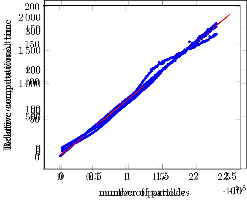
(d) representation formula

Figure 1: Single-core timings relative to 1 000 particles for building the cluster basis in Fig. 1 ($2.7\cdot 10^{-3}$ s), the evaluation of $\underline{N}_{0}$ in Fig. 1 ($2.3\cdot 10^{-3}$ s), the particle field in Fig. 1 ($5.3\cdot 10^{-3}$ s) and the gradient of the representation formula in Fig. 1 ($1.4\cdot 10^{-1}$ s). The number of triangles is 1 280. Computations were performend on an Intel Xeon Gold 6154@3 GHz with icc 19. Relevant compiler flags are -Ofast -xHost.

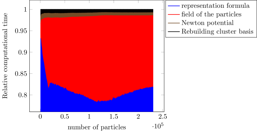
Figure 2: Cumulative computational times for 1 280 triangles and varying number of particles.

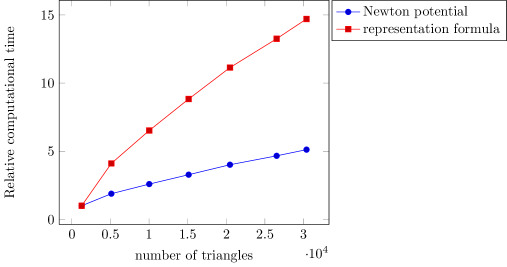
Figure 3: Single-core timings for different number of triangles relative to 1 280 triangles for 10 000 particles. The base values are $1.9\cdot 10^{-2}$ s and $1.4$ s for the Newton potential and representation formula, respectively. For information on the CPU and the compiler, see the caption of Fig. 1.

6.2 Physically motivated examples

For most applications the plasma contains positively and negatively charged particles. Usually, the positive charge exists of ionised atoms and electrons form the negatively charged part. Since the atoms are much heavier than the electrons they are modelled as immobile. This gives rise to a homogeneous positive background charge, such that the system is electrically neutral from the outside. The Poisson equation in (11) changes to

$$-\Delta_{x}\phi=\frac{1}{\beta}\left[1-w\sum\limits_{i=1}^{N_{p}}\delta^{\varepsilon}_{x_{i}}\right]$$

with boundary conditions

$$\phi =g_{D} \text{on }\Gamma_{D},$$

$$n_{\Omega}\cdot\nabla\phi =g_{N} \text{on }\Gamma_{N}.$$

Note that the integral of the right-hand side over $\Omega$ is zero, as $w=|\Omega|/N_{p}$. A particular solution for the homogeneous background charge is

$$\phi_{b}(x)=-\frac{1}{6\beta}|x|^{2}\quad x\in\Omega.$$

By subtracting traces of the particular solution $\phi_{b}$, we transform the boundary value problem to

$$-\Delta_{x}\phi_{e} =\frac{1}{\beta}w\sum\limits_{i=1}^{N_{p}}\delta_{x_{i}}$$

$$\phi_{e} =g_{D}-g_{b} \text{on }\Gamma_{D},$$

$$n_{\Omega}\cdot\nabla\phi_{e} =g_{N}-n_{\Omega}\cdot\nabla\phi_{b} \text{on }\Gamma_{N}.$$

The electric field is now obtained by

$$E=-\nabla\phi_{e}-\nabla\phi_{b}.$$

As $\phi_{b}$ is independent of the geometry and the distribution of the particles, its evaluation and the evaluation of its gradient are grid-free, as well as the computation of $\phi_{e}$. Computations with background charge can be found in Section 6.2.2 and Section 6.2.3.

6.2.1 Accelerator

As a first example for non-trivial boundary conditions, we consider an accelerator geometry, meshed with 8 904 triangles. The physically relevant parameters are $L_{0}=0.1\,\text{m}$, $n_{0}=10^{12}\,\text{m}^{-3}$ and $k_{B}T_{0}=1\,\text{eV}$. The profile of the rotationally symmetric accelerator and the boundary conditions for the electric potential are depicted in Fig. 4. Initially, 10 000 particles are placed in the left cylinder with a bulk velocity of 10 in positive $x$-direction and are absorbed at the boundary. Once they pass the first narrow, called screen, they are focused such that they pass the second narrow, the accelerator, without being absorbed by the boundaries. The distribution of 3 000 particles after 100 time steps with a time step size of $10^{-3}$ is shown in Fig. 5.

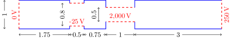
Figure 4: Profile of the accelerator along the $x$-axis. On the solid blue parts, homogeneous Neumann conditions are imposed. The voltages along the dashed red lines indicate the value of the Dirichlet boundary condition on these segments.

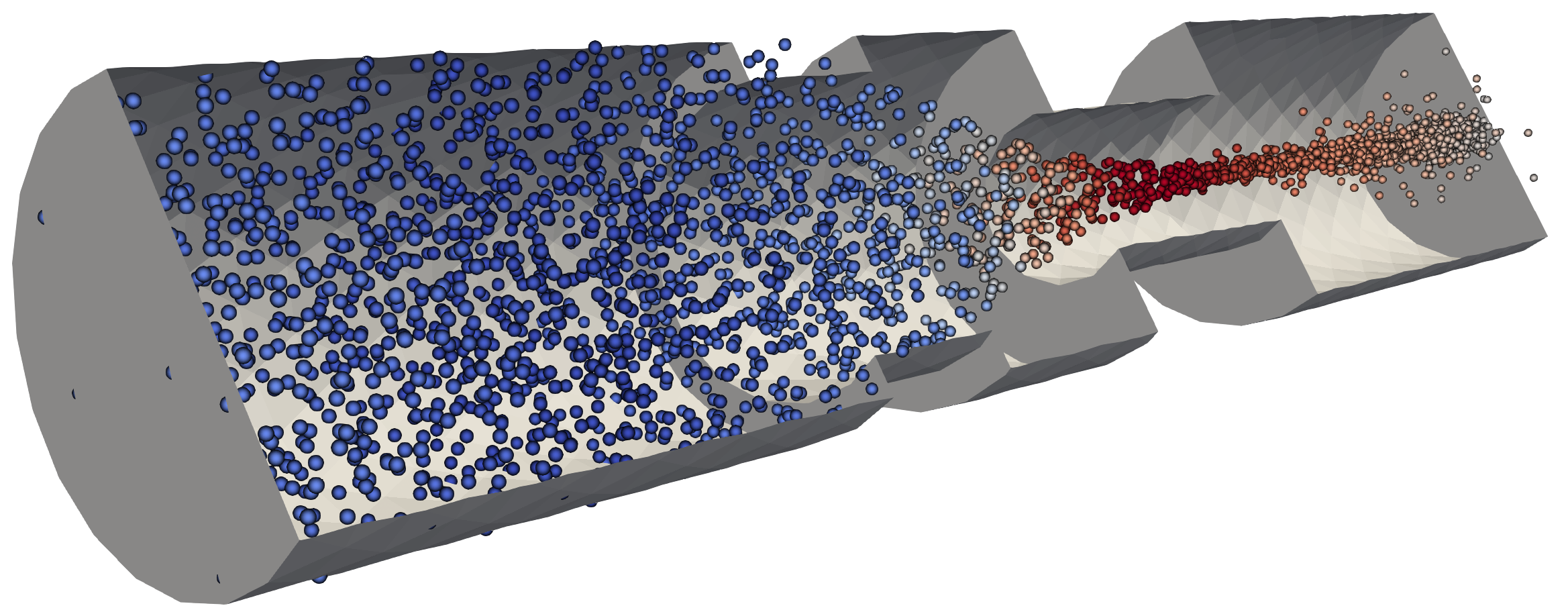
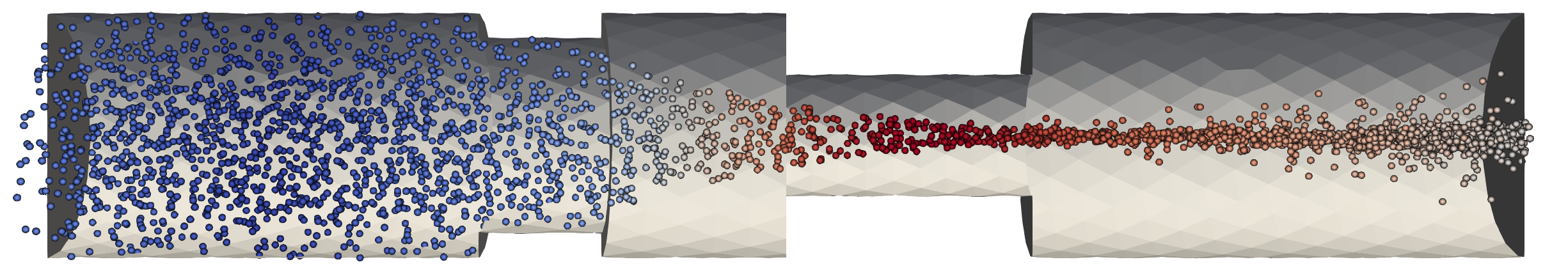
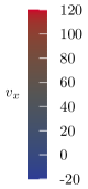
Figure 5: Final distribution of 3 000 particles inside the accelerator. The colour indactes the velocity of the particles in $x$-direction.

6.2.2 Plasma oscillations

As a first example with a homogeneous background charge, we examine plasma oscillations. The geometry is a cylinder along the $z$-axis with radius 1 and height 5, centered in $0$. It is discretised with 2 110 triangles. The characteristic quantities are $L_{0}=0.1\,\text{m}$, $n_{0}=10^{12}\,\text{m}^{-3}$ and $k_{B}T_{0}=1\,\text{eV}$. 5 000 particles are distributed uniformly in a smaller cylinder of height 4 around the centre of the geometry. Their initial velocities are set to $0$. The boundary is absorbing; at the bases we set homogeneous Dirichlet conditions and homogeneous Neumann conditions on the rest. Phyiscally, the latter boundary condition means that we impose a vanishing surface charge density, in particular there is no net charge on this part of the boundary. Mathematically, since the normal vectors point in radial direction, the condition

$$0=\gamma_{1}\phi=n_{\Omega}\cdot\gamma_{0}\nabla\phi=-n_{\Omega}\cdot\gamma_{0}E$$

ensures that the field lines close to the boundary are parallel to the cylinder axis. To prevent the particles from being absorbed at the lateral surface of the cylinder, we add a constant magnetic field in the order of $10\,\text{mT}$ along the $z$-axis. The acceleration due to the magnetic field is computed with the Boris scheme [6, 7] using a time step size of $10^{-4}$. In an infinite system, the plasma oscillates with the plasma frequency

$$\omega_{p}=\sqrt{\frac{n_{0}e^{2}}{\varepsilon_{0}m_{e}}},$$

which depends only on the electron density. As we simulate the plasma in a bounded domain, we cannot expect the plasma to oscillate with the frequency $\omega_{p}$. Instead, we validate that the frequency for the bounded domain is still a function of the square root of $n_{0}$. In order to do so, we vary the electron density $n$ from $n_{0}$ to $100n_{0}$. Counting the number of particles in three parts of the cylinder, $z\in[-2.5,2]$, $z\in[-0.25,0.25]$ and $z\in[2,2.5]$ at each time step, we extract the dominating non-zero frequency after with the help of the Discrete Fourier Transform. The numbers of particles in the left, the middle and right part of the cylinder for $n=10n_{0}$ is shown in Fig. 6. The distribution of the particles oscillates with dominating frequency of $12$ in units of $1/t_{0}$, which corresponds to a angular frequency of

$$\omega_{c}=3.2\cdot 10^{8}\,\frac{1}{\text{s}}$$

in physical units. This is in the order of the plasma frequency

$$\omega_{p}=\sqrt{\frac{10n_{0}e^{2}}{\varepsilon_{0}m_{e}}}\approx 1.8\cdot 10^{8}\,\frac{1}{\text{s}}.$$

The spectra of the lines in Fig. 6 only differ in magnitude, not in the positions of peaks. Therefore, we only show the spectrum of the second line of Fig. 6 in Fig. 7. Repeating this several densities between $n_{0}$ and $100n_{0}$ yields Fig. 8, from which the dependency of the frequency on the square root of the density is clearly deduced.

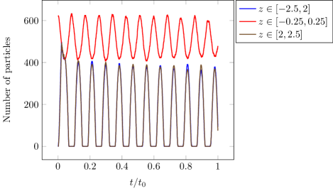
Figure 6: Number of particles in three parts of the cylinder over time for $n=10n_{0}$.

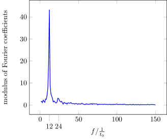
Figure 7: Fourier spectrum of the number of particles in the middle of the cylinder, the red line in Fig. 6. The constant mode is excluded from the spectrum.

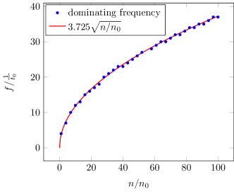
Figure 8: Frequency of the oscillation of the number of particles in the middle of the cylinder as a function of the electron density.

6.2.3 Plasma sheath

A classical nonlinear phenomenon in plasma physics is the formation of sheaths, see the classical textbook [14]. For this example, we set $L_{0}=0.1\,\text{m}$, $n_{0}=10^{13}\,\text{m}^{-3}$ and $k_{B}T_{0}=1\,\text{eV}$. We uniformly distribute 10 000 particles with velocity following a Maxwellian distribution with temperature 1 and bulk velocity 0 within the unit sphere, which is discretised with 1 280 triangles. The particles are absorbed at the boundary; for the electric potential, we impose homogeneous Dirichlet boundary conditions. The system is evolved with a time step size of $10^{-3}$. Fig. 9 shows the number of particles within the unit sphere as a function of time. At the beginning, the fastest particles leave the sphere, giving rise to a positive charge at the boundary. With the growing potential barrier, the particles are excluded from a thin area near the boundary, the so called sheath, and are confined inside the sphere. Figure 10 includes the final radial distribution function of the particles inside the sphere and the analytical radial distribution function of a uniformly distributed random variate inside the unit sphere. While the final positions are still uniformly distributed up to a radius of approximately $0.6$, the distribution strongly deviates from the uniform distribution especially close to radii of $1$, where it suddenly drops to $0$.

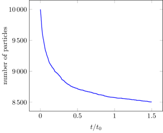
Figure 9: Number of particles inside the sphere over time.

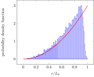
Figure 10: Radial histogram of the final particle distribution inside the sphere. The solid red line shows the probability density function of the uniform distribution.

6.3 Summary

To summarise, the numerical examples show that we are capable to simulate important non-linear plasma phenomena like plasma oscillations or the formation of sheaths. The results also match available theoretical predictions. Furthermore, the numerical study demonstrates the linear complexity of our method and its applicability on three-dimensional domains with mixed boundary values. The efficiency and flexibility of our approach open the possibilities for future simulations of complex problems in different plasma regimes.

References

- [1] A. W. Appel, An efficient program for many-body simulation, SIAM J. Sci. Statist. Comput., 6 (1985), pp. 85–103.
- [2] J. Barnes and P. Hut, A hierarchical force-calculation algorithm, Nature, 324 (1986), pp. 446–449.
- [3] M. Bebendorf, Approximation of boundary element matrices, Numer. Math., 86 (2000), pp. 565–589.
- [4] M. Bebendorf, Hierarchical Matrices, vol. 63 of Lecture Notes in Computational Science and Engineering, Springer, Berlin Heidelberg, 2008.
- [5] M. Bebendorf and S. Rjasanow, Adaptive low-rank approximation of collocation matrices, Computing, 70 (2003), pp. 1–24.
- [6] C. Birdsall and A. A.B Langdon, Plasma Physics via Computer Simulation, Series in Plasma Physics, Taylor & Francis Group, New York, 2005.
- [7] J. Boris, The acceleration calculation from a scalar potential, tech. report, Plasma Physics Laboratory, Princeton University MATT-152, 1970.
- [8] S. Börm, Efficient Numerical Methods for Non-local Operators, vol. 14 of EMS Tracts in Mathematics, European Mathematical Society, 2010.
- [9] S. Börm and S. Christophersen, Approximation of integral operators by Green quadrature and nested cross approximation, Numer. Math., 133 (2016), pp. 409–442.
- [10] S. Börm and L. Grasedyck, Low-rank approximation of integral operators by interpolation, Computing, 72 (2004), pp. 325–332.
- [11] S. Börm and L. Grasedyck, Hybrid cross approximation of integral operators, Numer. Math., 101 (2005).
- [12] S. Börm, M. Löhndorf, and J. M. Melenk, Approximation of integral operators by variable-order interpolation, Numer. Math., 99 (2005), pp. 605–643.
- [13] J. Carrier, L. Greengard, and V. Rokhlin, A fast adaptive multipole algorithm for particle simulations, SIAM J. Sci. Statist. Comput., 9 (1988), pp. 669–686.
- [14] F. F. Chen, Introduction to Plasma Physics and Controlled Fusion, Springer International Publishing, 2016.
- [15] H. Cheng, L. Greengard, and V. Rokhlin, A fast adaptive multipole algorithm in three dimensions, J. Comput. Phys., 155 (1999), pp. 468–498.
- [16] A. Christlieb, R. Krasny, J. Verboncoeur, J. Emhoff, and I. Boyd, Grid-free plasma simulation techniques, IEEE T Plasma Sci, 34 (2006), pp. 149–165.
- [17] A. J. Christlieb and K. Cartwright, Boundary integral corrected particle-in-cell, in 2008 IEEE 35th International Conference on Plasma Science, 2008.
- [18] A. J. Christlieb, R. Krasny, and J. Verboncoeur, Efficient particle simulation of a virtual cathode using a grid-free treecode Poisson solver, IEEE Transactions on Plasma Science, 32 (2004), pp. 384–389.
- [19] A. J. Christlieb, R. Krasny, and J. P. Verboncoeur, A treecode algorithm for simulating electron dynamics in a Penning-Malmberg trap, Computer Physics Communications, 164 (2004), pp. 306–310.
- [20] T. Darden, D. York, and L. Pedersen, Particle mesh Ewald: An N log(N) method for Ewald sums in large systems, J. Chem. Phys., 98 (1993), pp. 10089–10092.
- [21] J. M. Dawson, Particle simulation of plasmas, Rev. Mod. Phys., 55 (1983), pp. 403–447.
- [22] K. Ganguly and H. D. Victory, Jr., On the convergence of particle methods for multidimensional Vlasov-Poisson systems, SIAM J. Numer. Anal., 26 (1989), pp. 249–288.
- [23] L. Greengard and V. Rokhlin, A fast algorithm for particle simulations, J. Comput. Phys., 73 (1987), pp. 325–348.
- [24] L. Greengard and V. Rokhlin, The rapid evaluation of potential fields in three dimensions, in Vortex Methods, C. Anderson and C. Greengard, eds., vol. 1360 of Lecture Notes in Mathematics, Springer, 1988, pp. 121–141.
- [25] L. Greengard and V. Rokhlin, A new version of the fast multipole method for the Laplace equation in three dimensions, in Acta numerica, 1997, vol. 6 of Acta Numer., Cambridge Univ. Press, Cambridge, 1997, pp. 229–269.
- [26] W. Hackbusch, Hierarchical Matrices: Algorithms and Analysis, vol. 49 of Springer Series in Computational Mathematics, Springer, Berlin, Heidelberg, 2015.
- [27] R. Hockney and J. Eastwood, Computer Simulation Using Particles, CRC Press, 1988.
- [28] V. Kolobov and R. Arslanbekov, Electrostatic PIC with adaptive cartesian mesh, Journal of Physics: Conference Series, 719 (2016), p. 012020.
- [29] D. Lazarovici and P. Pickl, A mean field limit for the Vlasov-Poisson system, Arch. Ration. Mech. Anal., 225 (2017), pp. 1201–1231.
- [30] W. C. H. McLean, Strongly elliptic systems and boundary integral equations, Cambridge University Press, Cambridge, 2000.
- [31] H. Neunzert, An introduction to the nonlinear Boltzmann-Vlasov equation, in Kinetic theories and the Boltzmann equation (Montecatini, 1981), vol. 1048 of Lecture Notes in Mathematics, Springer, Berlin, 1984, pp. 60–110.
- [32] H. Neunzert and J. Wick, Theoretische und numerische Ergebnisse zur nichtlinearen Vlasov-Gleichung, in Numerische Lösung nichtlinearer partieller Differential- und Integrodifferentialgleichungen (Tagung Math. Forschungsinst., Oberwolfach, 1971), vol. 267 of Lecture Notes in Mathematics, Springer, Berlin, 1972, pp. 159–185.
- [33] H. Neunzert and J. Wick, Die Theorie der asymptotischen Verteilung und die numerische Lösung von Integrodifferentialgleichungen, Numer. Math., 21 (1973/74), pp. 234–243.
- [34] H. Neunzert and J. Wick, Die Approximation der Lösung von Integro-Differentialgleichungen durch endliche Punktmengen, in Numerische Behandlung nichtlinearer Integrodifferential- und Differentialgleichungen (Tagung, Math. Forschungsinst., Oberwolfach, 1973), 1974, pp. 275–290. Lecture Notes in Mathematics, Vol. 395.
- [35] D. R. Nicholson, Introduction to Plasma Theory, Wiley, 1983.
- [36] C. Nieter, J. R. Cary, G. R. Werner, D. N. Smithe, and P. H. Stoltz, Application of Dey–Mittra conformal boundary algorithm to 3d electromagnetic modeling, Journal of Computational Physics, 228 (2009), pp. 7902 – 7916.
- [37] G. Of, O. Steinbach, and P. Urthaler, Fast evaluation of volume potentials in boundary element methods, SIAM J. Sci. Comput., 32 (2010), pp. 585–602.
- [38] G. Of, O. Steinbach, and W. L. Wendland, Applications of a fast multipole Galerkin in boundary element method in linear elastostatics, Comput. Vis. Sci., 8 (2005), pp. 201–209.
- [39] G. Of, O. Steinbach, and W. L. Wendland, The fast multipole method for the symmetric boundary integral formulation, IMA J. Numer. Anal., 26 (2006), pp. 272–296.
- [40] S. Rjasanow and O. Steinbach, The fast solution of boundary integral equations, Mathematical and Analytical Techniques with Applications to Engineering, Springer, New York, 2007.
- [41] S. Sauter and C. Schwab, Boundary Element Methods, vol. 39 of Springer Series in Computational Mathematics, Springer, Berlin, Heidelberg, 2011.
- [42] H. Spohn, Large Scale Dynamics of Interacting Particles, Springer, Berlin, Heidelberg, 1991.
- [43] O. Steinbach, Numerical approximation methods for elliptic boundary value problems: finite and boundary elements, Springer, New York, 2007.
- [44] J. P. Verboncoeur, Particle simulation of plasmas: review and advances, Plasma Physics and Controlled Fusion, 47 (2005), pp. A231–A260.
- [45] S. Wollman, On the approximation of the Vlasov-Poisson system by particle methods, SIAM J. Numer. Anal., 37 (2000), pp. 1369–1398.
- [46] L. Ying, G. Biros, and D. Zorin, A kernel-independent adaptive fast multipole algorithm in two and three dimensions, J. Comput. Phys., 196 (2004), pp. 591–626.