A new method for suppressing excited-state contaminations on the nucleon form factors

Harvey B.ย Meyer, Konstantin Ottnad and
PRISMA Cluster of Excellence, Institut fรผr Kernphysik and Helmholtz Institut Mainz,
Johannes Gutenberg-Universitรคt Mainz, 55099 Mainz, Germany
E-mail
Abstract:

One of the most challenging tasks in lattice calculations of baryon form factors is the analysis and control of excited-state contaminations. Taking the isovector axial form factors of the nucleon as an example, both a dispersive representation and a calculation in chiral effective field theory show that the excited-state contributions become dominant at fixed source-sink separation when the axial current is spatially distant from the nucleon source location. We address this effect with a new method in which the axial current is localized by a Gaussian wave-packet and apply it on a CLS ensemble with $N_{f}=2+1$ flavors of O($a$) improved Wilson fermions with a pion mass of $m_{\pi}=200\,$MeV.

1 Introduction

The study of the electroweak form factors of the nucleon reveals insights into its internal structure. Electron scattering and atomic spectroscopy can be used to probe the electromagnetic form factors $G_{E}(q^{2}),G_{M}(q^{2})$, whereas for the study of the axial form factors $G_{A}(q^{2}),G_{P}(q^{2})$, which are far less well known than the electromagnetic form factors [1], one has to rely on weak probes, i.e.ย neutrino scattering or muon capture processes. Although there is a formal description of the strong interaction given by the theory of Quantum chromodynamics (QCD), it remains highly challenging to understand the details of low-energy phenomena of hadronic bound states such as the proton. To this day, many aspects about the distribution of the proton charge and spin as well as the contribution of the gluons to the proton spin are not understood at a satisfactory level.

Phenomenologically, the nucleon axial charge $g_{A}=G_{A}(0)$ is known to two parts per mille from neutron beta decay. In comparison, lattice QCD studies of this low-energy observable still suffer from large statistical and systematic uncertaintiesย [2]. One of the main sources for the latter is the contamination of the relevant correlation functions from excited-state contributions. Here we investigate a new method to overcome this problem by localizing the axial-vector current in position space.

2 Formalism of nucleon correlation functions

We start with the Euclidean nucleon two- and three-point correlation functions, given by

C2โ€‹(pโ†’,ts)subscript๐ถ2โ†’๐‘subscript๐‘ก๐‘ \displaystyle C_{2}(\vec{p},t_{s}) =a3โ€‹โˆ‘xโ†’eโˆ’iโ€‹pโ†’โ‹…xโ†’โ€‹ฮ“ฮฒโ€‹ฮฑโ€‹โŸจ๐’ฉฮฑโ€‹(xโ†’,ts)โ€‹๐’ฉยฏฮฒโ€‹(0)โŸฉ,absentsuperscript๐‘Ž3subscriptโ†’๐‘ฅsuperscript๐‘’โ‹…๐‘–โ†’๐‘โ†’๐‘ฅsubscriptฮ“๐›ฝ๐›ผdelimited-โŸจโŸฉsubscript๐’ฉ๐›ผโ†’๐‘ฅsubscript๐‘ก๐‘ subscriptยฏ๐’ฉ๐›ฝ0\displaystyle=a^{3}\sum_{\vec{x}}e^{-i\vec{p}\cdot\vec{x}}\,\Gamma_{\beta\alpha}\langle\mathcal{N}_{\alpha}(\vec{x},t_{s})\mathcal{\bar{N}}_{\beta}(0)\rangle, (1)
C3,๐’ชโ€‹(pโ†’,pโ†’โ€ฒ,t,ts)subscript๐ถ3๐’ชโ†’๐‘superscriptโ†’๐‘โ€ฒ๐‘กsubscript๐‘ก๐‘ \displaystyle C_{3,\mathcal{O}}(\vec{p},\vec{p}^{\prime},t,t_{s}) =a6โ€‹โˆ‘xโ†’,yโ†’eiโ€‹(pโ†’โ€ฒโˆ’pโ†’)โ‹…yโ†’โ€‹eโˆ’iโ€‹pโ†’โ€ฒโ‹…xโ†’โ€‹ฮ“ฮฒโ€‹ฮฑโ€‹โŸจ๐’ฉฮฑโ€‹(xโ†’,ts)โ€‹๐’ชโ€‹(yโ†’,t)โ€‹๐’ฉยฏฮฒโ€‹(0)โŸฉ.absentsuperscript๐‘Ž6subscriptโ†’๐‘ฅโ†’๐‘ฆsuperscript๐‘’โ‹…๐‘–superscriptโ†’๐‘โ€ฒโ†’๐‘โ†’๐‘ฆsuperscript๐‘’โ‹…๐‘–superscriptโ†’๐‘โ€ฒโ†’๐‘ฅsubscriptฮ“๐›ฝ๐›ผdelimited-โŸจโŸฉsubscript๐’ฉ๐›ผโ†’๐‘ฅsubscript๐‘ก๐‘ ๐’ชโ†’๐‘ฆ๐‘กsubscriptยฏ๐’ฉ๐›ฝ0\displaystyle=a^{6}\sum_{\vec{x},\vec{y}}e^{i(\vec{p}^{\prime}-\vec{p})\cdot\vec{y}}e^{-i\vec{p}^{\prime}\cdot\vec{x}}\,\Gamma_{\beta\alpha}\langle\mathcal{N}_{\alpha}(\vec{x},t_{s})\mathcal{O}(\vec{y},t)\mathcal{\bar{N}}_{\beta}(0)\rangle. (2)

The source-sink separation tssubscript๐‘ก๐‘ t_{s} measures the Euclidean time between the nucleon creation (source) and annihilation (sink) point. A local operator is inserted at space-time position $y=(\vec{y},t)$, 0โ‰คtโ‰คts0๐‘กsubscript๐‘ก๐‘ 0\leq t\leq t_{s}, which has a nucleon matrix element given by โŸจN,pโ†’โ€ฒ,sโ€ฒ|๐’ชโ€‹(0)|N,pโ†’,sโŸฉ=uยฏsโ€ฒโ€‹(pโ†’โ€ฒ)โ€‹๐’ชโ€‹(P,Q)โ€‹usโ€‹(pโ†’)quantum-operator-product๐‘superscriptโ†’๐‘โ€ฒsuperscript๐‘ โ€ฒ๐’ช0๐‘โ†’๐‘๐‘ superscriptยฏ๐‘ขsuperscript๐‘ โ€ฒsuperscriptโ†’๐‘โ€ฒ๐’ช๐‘ƒ๐‘„superscript๐‘ข๐‘ โ†’๐‘\langle N,\vec{p}^{\prime},s^{\prime}|\mathcal{O}(0)|N,\vec{p},s\rangle=\bar{u}^{s^{\prime}}(\vec{p}^{\prime})\mathcal{O}(P,Q)u^{s}(\vec{p}), $P\equiv p^{\prime}+p$, $Q\equiv p^{\prime}-p$. Taking the limit t,(tsโˆ’t)โ‰ซmฯ€โˆ’1much-greater-than๐‘กsubscript๐‘ก๐‘ ๐‘กsuperscriptsubscript๐‘š๐œ‹1t,(t_{s}-t)\gg m_{\pi}^{-1} and performing a spectral decomposition, one obtains (NB: we use Euclidean Dirac matrices, $\{\gamma_{\mu},\gamma_{\nu}\}=2\delta_{\mu\nu}$)

$\displaystyle C_{2}(\vec{p},t)$ $\displaystyle=e^{-E_{\vec{p}}t}|Z(\vec{p})|^{2}\left(1+\frac{m_{N}}{E_{\vec{p}}}\right)+\dots,$ (3)
C3,๐’ชโ€‹(pโ†’,pโ†’โ€ฒ,t,ts)subscript๐ถ3๐’ชโ†’๐‘superscriptโ†’๐‘โ€ฒ๐‘กsubscript๐‘ก๐‘ \displaystyle C_{3,\mathcal{O}}(\vec{p},\vec{p}^{\prime},t,t_{s}) =Zโ€‹(pโ†’โ€ฒ)โ€‹Zโˆ—โ€‹(pโ†’)4โ€‹Epโ†’โ€‹Epโ†’โ€ฒโ€‹eโˆ’Epโ†’โ€ฒโ€‹(tsโˆ’t)โ€‹eโˆ’Epโ†’โ€‹tโ€‹Trโ€‹(ฮ“โ€‹(โˆ’iโ€‹pฬธโ€ฒ+m)โ€‹๐’ชโ€‹(P,Q)โ€‹(โˆ’iโ€‹pฬธ+m))+โ€ฆ,absent๐‘superscriptโ†’๐‘โ€ฒsuperscript๐‘โ†’๐‘4subscript๐ธโ†’๐‘subscript๐ธsuperscriptโ†’๐‘โ€ฒsuperscript๐‘’subscript๐ธsuperscriptโ†’๐‘โ€ฒsubscript๐‘ก๐‘ ๐‘กsuperscript๐‘’subscript๐ธโ†’๐‘๐‘กTrฮ“๐‘–superscriptitalic-pฬธโ€ฒ๐‘š๐’ช๐‘ƒ๐‘„๐‘–italic-pฬธ๐‘šโ€ฆ\displaystyle=\frac{Z(\vec{p}^{\prime})Z^{*}(\vec{p})}{4E_{\vec{p}}E_{\vec{p}^{\prime}}}e^{-E_{\vec{p}^{\prime}}(t_{s}-t)}e^{-E_{\vec{p}}t}\,\text{Tr}\left(\Gamma(-i\not{p}^{\prime}+m)\mathcal{O}(P,Q)(-i\not{p}+m)\right)+\dots, (4)

where the dots stand for excited-state contributions and $p_{0}=iE_{\vec{p}}=i\sqrt{\vec{p}^{2}+m_{N}^{2}}$, $p_{0}^{\prime}=iE_{\vec{p}^{\prime}}$.

It is interesting to compare the expression

C^3,๐’ชโ€‹(pโ†’,pโ†’โ€ฒ,t,ts)โ‰กZโ€‹(pโ†’โ€ฒ)โ€‹Zโˆ—โ€‹(pโ†’)โ€‹โˆซโˆ’โˆžโˆždโ€‹p02โ€‹ฯ€โ€‹โˆซโˆ’โˆžโˆždโ€‹p0โ€ฒ2โ€‹ฯ€โ€‹Trโ€‹{ฮ“โ€‹โˆ’iโ€‹pฬธโ€ฒ+mpโ€ฒ+2m2โ€‹๐’ชโ€‹(P,Q)โ€‹โˆ’iโ€‹pฬธ+mp2+m2}โ€‹eiโ€‹p0โ€ฒโ€‹(tsโˆ’t)+iโ€‹p0โ€‹t\hat{C}_{3,\mathcal{O}}(\vec{p},\vec{p}^{\prime},t,t_{s})\equiv Z(\vec{p}^{\prime})Z^{*}(\vec{p})\int_{-\infty}^{\infty}\frac{dp_{0}}{2\pi}\int_{-\infty}^{\infty}\frac{dp_{0}^{\prime}}{2\pi}{\rm Tr}\Big{\{}\Gamma\frac{-i\not{p}^{\prime}+m}{p^{\prime}{}^{2}+m^{2}}{\cal O}(P,Q)\frac{-i\not{p}+m}{p^{2}+m^{2}}\Big{\}}e^{ip_{0}^{\prime}(t_{s}-t)+ip_{0}t} (5)

to Eq.ย (4). Performing the $p_{0},p_{0}^{\prime}$ integrals by contour integration, the function $\hat{C}_{3,\mathcal{O}}$ is found to contain the ground-state contribution of $C_{3,\mathcal{O}}$, but it also contains additional terms due to the singularities of the form factor in the complex plane. What makes $\hat{C}_{3,\mathcal{O}}$ appealing is that, for Lorentz-covariant interpolating operators ($Z(\vec{p})$ independent of $\vec{p}$), it has a manifestly Lorentz-covariant form, which the ground-state contribution in (4) does not111This observation is most easily made by Fourier-transforming $\hat{C}_{3,\mathcal{O}}$ with respect to $\vec{p}$ and $\vec{p}^{\prime}$ to obtain the coordinate-space three-point function.. Thus it appears that $\hat{C}_{3,\mathcal{O}}$ is a Lorentz-covariant completion of the ground-state contribution to $C_{3,\mathcal{O}}$.

Consider then the case of ${\cal O}=A_{\mu}^{a}=\bar{\psi}\gamma_{\mu}\gamma_{5}\frac{\tau^{a}}{2}\psi$ the isovector axial current, for which ${\cal O}(P,Q)=\left[\gamma_{\mu}\gamma_{5}G_{A}(-Q^{2})-i\gamma_{5}\frac{Q_{\mu}}{2m_{N}}G_{P}(-Q^{2})\right]\frac{\tau^{a}}{2}$ is parametrized by the axial and induced-pseudoscalar form factors, and does not depend on $P$. To exhibit the singularities of the form factors, we use their dispersive representation,

GA,Pโ€‹(โˆ’Q2)=โˆซs0โˆždโ€‹sฯ€โ€‹Imโ€‹GA,Pโ€‹(s)s+Q2.subscript๐บ๐ด๐‘ƒsuperscript๐‘„2superscriptsubscriptsubscript๐‘ 0๐‘‘๐‘ ๐œ‹Imsubscript๐บ๐ด๐‘ƒ๐‘ ๐‘ superscript๐‘„2G_{A,P}(-Q^{2})=\int_{s_{0}}^{\infty}\frac{ds}{\pi}\frac{{\rm Im\,}G_{A,P}(s)}{s+Q^{2}}. (6)

Inserting these expressions into Eq.ย (5), the additional terms generated can be analyzed more explicitly. In the present case, the induced pseudoscalar form factor contains a pole at s0=mฯ€2subscript๐‘ 0superscriptsubscript๐‘š๐œ‹2s_{0}=m_{\pi}^{2}, while the axial current has a three-pion threshold at s0=9โ€‹mฯ€2subscript๐‘ 09superscriptsubscript๐‘š๐œ‹2s_{0}=9m_{\pi}^{2}. Keeping only the pion-pole contribution to the three-point function,

Imโ€‹GPโ€‹(s)=4โ€‹ฯ€โ€‹MN2โ€‹gAฯ€โ€‹ฮดโ€‹(sโˆ’mฯ€2)+โ€ฆ,Imsubscript๐บ๐‘ƒ๐‘ 4๐œ‹superscriptsubscript๐‘€๐‘2superscriptsubscript๐‘”๐ด๐œ‹๐›ฟ๐‘ superscriptsubscript๐‘š๐œ‹2โ€ฆ{\rm Im\,}G_{P}(s)=4\pi M_{N}^{2}g_{A}^{\pi}\delta(s-m_{\pi}^{2})+\dots, (7)

we obtain for the case of ${\cal O}=A_{0}^{3}$ in the proton with $\vec{p}^{\prime}=0$ and ฮ“=12โ€‹(1+ฮณ0)โ€‹(1+iโ€‹ฮณ5โ€‹sโ†’โ‹…ฮณโ†’)ฮ“121subscript๐›พ01โ‹…๐‘–subscript๐›พ5โ†’๐‘ โ†’๐›พ\Gamma=\frac{1}{2}(1+\gamma_{0})(1+i\gamma_{5}\,\vec{s}\cdot\vec{\gamma}),

C^3,A0โ€‹(โˆ’qโ†’,0โ†’,t,ts)ฯ€โ€‹pole=Zโ€‹(0โ†’)โ€‹Zโˆ—โ€‹(โˆ’qโ†’)โ€‹MNโ€‹gAฯ€โ€‹sโ†’โ‹…qโ†’Eqโ†’subscript^๐ถ3subscript๐ด0subscriptโ†’๐‘žโ†’0๐‘กsubscript๐‘ก๐‘ ๐œ‹poleโ‹…๐‘โ†’0superscript๐‘โ†’๐‘žsubscript๐‘€๐‘superscriptsubscript๐‘”๐ด๐œ‹โ†’๐‘ โ†’๐‘žsubscript๐ธโ†’๐‘ž\displaystyle\hat{C}_{3,A_{0}}(-\vec{q},\vec{0},t,t_{s})_{\pi~{}{\rm pole}}=\frac{Z(\vec{0})Z^{*}(-\vec{q})\,M_{N}g_{A}^{\pi}\,\vec{s}\cdot\vec{q}}{E_{\vec{q}}} (8)
[2โ€‹Eqโ†’โ€‹eโˆ’MNโ€‹tsโˆ’ฯ‰qโ†’โ€‹t(MN+ฯ‰qโ†’)2โˆ’Eqโ†’2โˆ’eโˆ’Eqโ†’โ€‹tsโˆ’ฯ‰qโ†’โ€‹(tsโˆ’t)ฯ‰qโ†’+Eqโ†’โˆ’MN+2โ€‹(MNโˆ’Eqโ†’)โ€‹eโˆ’Eqโ†’โ€‹tโˆ’MNโ€‹(tsโˆ’t)ฯ‰qโ†’2โˆ’(Eqโ†’โˆ’MN)2].delimited-[]2subscript๐ธโ†’๐‘žsuperscript๐‘’subscript๐‘€๐‘subscript๐‘ก๐‘ subscript๐œ”โ†’๐‘ž๐‘กsuperscriptsubscript๐‘€๐‘subscript๐œ”โ†’๐‘ž2superscriptsubscript๐ธโ†’๐‘ž2superscript๐‘’subscript๐ธโ†’๐‘žsubscript๐‘ก๐‘ subscript๐œ”โ†’๐‘žsubscript๐‘ก๐‘ ๐‘กsubscript๐œ”โ†’๐‘žsubscript๐ธโ†’๐‘žsubscript๐‘€๐‘2subscript๐‘€๐‘subscript๐ธโ†’๐‘žsuperscript๐‘’subscript๐ธโ†’๐‘ž๐‘กsubscript๐‘€๐‘subscript๐‘ก๐‘ ๐‘กsuperscriptsubscript๐œ”โ†’๐‘ž2superscriptsubscript๐ธโ†’๐‘žsubscript๐‘€๐‘2\displaystyle\Big{[}\frac{2E_{\vec{q}}\,e^{-M_{N}t_{s}-\omega_{\vec{q}}\,t}}{(M_{N}+\omega_{\vec{q}})^{2}-E_{\vec{q}}^{2}}-\frac{e^{-E_{\vec{q}}\,t_{s}-\omega_{\vec{q}}(t_{s}-t)}}{\omega_{\vec{q}}+E_{\vec{q}}-M_{N}}+\frac{2(M_{N}-E_{\vec{q}})e^{-E_{\vec{q}}\,t-M_{N}(t_{s}-t)}}{\omega_{\vec{q}}^{2}-(E_{\vec{q}}-M_{N})^{2}}\Big{]}.

From the time-dependence of the last term, one identifies it with the ground-state contribution; its denominator is nothing but $Q^{2}+m_{\pi}^{2}$, thus corresponding to the pion-pole contribution to $G_{\rm P}$. The other terms are subdominant for large t,tsโˆ’t๐‘กsubscript๐‘ก๐‘ ๐‘กt,t_{s}-t; they represent $N\pi$ excited-state contributions.

In order to confirm this interpretation, one may calculate the pion-exchange contribution to C3,Aฮผโ€‹(pโ†’,pโ†’โ€ฒ,t,ts)subscript๐ถ3subscript๐ด๐œ‡โ†’๐‘superscriptโ†’๐‘โ€ฒ๐‘กsubscript๐‘ก๐‘ C_{3,A_{\mu}}(\vec{p},\vec{p}^{\prime},t,t_{s}) in chiral effective theory (ChEFT), using the representation $A_{\mu}^{a}=-2if\partial_{\mu}\pi^{a}+\dots$, with $f$ the pion decay constant, and the interaction Lagrangian

$\displaystyle\mathcal{L}_{\text{int}}$ $\displaystyle=\frac{ig_{A}}{f}\bar{\Psi}(x)\gamma_{\mu}\gamma_{5}\frac{\tau^{a}}{2}\Psi(x)\partial_{\mu}\pi^{a}(x).$ (9)

A straightforward field-theoretic calculation then gives

C3,A0โ€‹(โˆ’qโ†’,0โ†’,t,ts)ChEFT,ฯ€โ€‹exchange=|Z|2โ€‹gAโ€‹sโ†’โ‹…qโ†’2โ€‹Eqโ†’subscript๐ถ3subscript๐ด0subscriptโ†’๐‘žโ†’0๐‘กsubscript๐‘ก๐‘ ChEFT๐œ‹exchangeโ‹…superscript๐‘2subscript๐‘”๐ดโ†’๐‘ โ†’๐‘ž2subscript๐ธโ†’๐‘ž\displaystyle C_{3,A_{0}}(-\vec{q},\vec{0},t,t_{s})_{\rm ChEFT,\pi~{}{\rm exchange}}=\frac{|Z|^{2}g_{A}\,\vec{s}\cdot\vec{q}}{2E_{\vec{q}}} (10)
[4โ€‹Eqโ†’โ€‹(MN+ฯ‰qโ†’)โ€‹eโˆ’MNโ€‹tsโˆ’ฯ‰qโ†’โ€‹t(MN+ฯ‰qโ†’)2โˆ’Eqโ†’2โˆ’(ฯ‰qโ†’+Eqโ†’+MN)โ€‹eโˆ’Eqโ†’โ€‹tsโˆ’ฯ‰qโ†’โ€‹(tsโˆ’t)ฯ‰qโ†’+Eqโ†’โˆ’MN+4โ€‹MNโ€‹(MNโˆ’Eqโ†’)โ€‹eโˆ’Eqโ†’โ€‹tโˆ’MNโ€‹(tsโˆ’t)ฯ‰qโ†’2โˆ’(Eqโ†’โˆ’MN)2].delimited-[]4subscript๐ธโ†’๐‘žsubscript๐‘€๐‘subscript๐œ”โ†’๐‘žsuperscript๐‘’subscript๐‘€๐‘subscript๐‘ก๐‘ subscript๐œ”โ†’๐‘ž๐‘กsuperscriptsubscript๐‘€๐‘subscript๐œ”โ†’๐‘ž2superscriptsubscript๐ธโ†’๐‘ž2subscript๐œ”โ†’๐‘žsubscript๐ธโ†’๐‘žsubscript๐‘€๐‘superscript๐‘’subscript๐ธโ†’๐‘žsubscript๐‘ก๐‘ subscript๐œ”โ†’๐‘žsubscript๐‘ก๐‘ ๐‘กsubscript๐œ”โ†’๐‘žsubscript๐ธโ†’๐‘žsubscript๐‘€๐‘4subscript๐‘€๐‘subscript๐‘€๐‘subscript๐ธโ†’๐‘žsuperscript๐‘’subscript๐ธโ†’๐‘ž๐‘กsubscript๐‘€๐‘subscript๐‘ก๐‘ ๐‘กsuperscriptsubscript๐œ”โ†’๐‘ž2superscriptsubscript๐ธโ†’๐‘žsubscript๐‘€๐‘2\displaystyle\Big{[}\frac{4E_{\vec{q}}(M_{N}+\omega_{\vec{q}})e^{-M_{N}t_{s}-\omega_{\vec{q}}\,t}}{(M_{N}+\omega_{\vec{q}})^{2}-E_{\vec{q}}^{2}}-\frac{(\omega_{\vec{q}}+E_{\vec{q}}+M_{N})\,e^{-\,E_{\vec{q}}\,t_{s}-\omega_{\vec{q}}\,(t_{s}-t)}}{\omega_{\vec{q}}+E_{\vec{q}}-M_{N}}+\frac{4M_{N}(M_{N}-E_{\vec{q}})\,e^{-\,E_{\vec{q}}\,t-M_{N}(t_{s}-t)}}{\omega_{\vec{q}}^{2}-(E_{\vec{q}}-M_{N})^{2}}\Big{]}.

The last term in the square bracket corresponds to the ground-state contribution and matches exactly the third term in Eq.ย (8) if we identify $g_{A}^{\pi}=g_{A}$. The first and second term of Eqs. (8) and (10) also agree in the limit of small $m_{\pi},|\vec{q}|$. In the ChEFT calculation222See [3] for a complete leading-order calculation in ChEFT; the pion-exchange contribution is found to be dominant., it is clear that these terms correspond to excited-state contributions. We conclude that $\hat{C}_{3,{\cal O}}$ can be helpful in describing the pre-asymptotic form of the three-point function, especially when a pole contribution is present. Importantly, it does not involve additional parameters as compared to the expression of the ground-state contribution, as it is determined by the same form factor.

2.1 Current insertion in coordinate-space

Performing a Fourier transform of equation (10) to localize the axial current at point $(t,\vec{y})$ in coordinate space yields the following expression,

โˆซd3โ€‹p(2โ€‹ฯ€)3โ€‹eiโ€‹pโ†’โ‹…yโ†’โ€‹C3,A0โ€‹(pโ†’,0โ†’,t,ts)ฯ€โ€‹exch.ChEFTsuperscript๐‘‘3๐‘superscript2๐œ‹3superscript๐‘’โ‹…๐‘–โ†’๐‘โ†’๐‘ฆsubscript๐ถ3subscript๐ด0subscriptsuperscriptโ†’๐‘โ†’0๐‘กsubscript๐‘ก๐‘ ChEFT๐œ‹exch\displaystyle\int\frac{d^{3}p}{(2\pi)^{3}}e^{i\vec{p}\cdot\vec{y}}C_{3,A_{0}}(\vec{p},\vec{0},t,t_{s})^{\rm ChEFT}_{\pi~{}{\rm exch.}} โ‰ˆ2โ€‹iโ€‹|Z|2โ€‹gAโ€‹eโˆ’mNโ€‹tsโ€‹sโ†’โ‹…โˆ‡โ†’yโ†’โ€‹[Gฯ€โ€‹(t,yโ†’)โˆ’Gฯ€โ€‹(tsโˆ’t,yโ†’)+mฯ€22โ€‹MNโ€‹eโˆ’mฯ€โ€‹|yโ†’|4โ€‹ฯ€โ€‹|yโ†’|],absentโ‹…2๐‘–superscript๐‘2subscript๐‘”๐ดsuperscript๐‘’subscript๐‘š๐‘subscript๐‘ก๐‘ โ†’๐‘ subscriptโ†’โˆ‡โ†’๐‘ฆdelimited-[]subscript๐บ๐œ‹๐‘กโ†’๐‘ฆsubscript๐บ๐œ‹subscript๐‘ก๐‘ ๐‘กโ†’๐‘ฆsuperscriptsubscript๐‘š๐œ‹22subscript๐‘€๐‘superscript๐‘’subscript๐‘š๐œ‹โ†’๐‘ฆ4๐œ‹โ†’๐‘ฆ\displaystyle\approx 2i|Z|^{2}g_{A}e^{-m_{N}t_{s}}\vec{s}\cdot\vec{\nabla}_{\vec{y}}\left[G_{\pi}(t,\vec{y})-G_{\pi}(t_{s}-t,\vec{y})+\frac{m_{\pi}^{2}}{2M_{N}}\frac{e^{-m_{\pi}|\vec{y}|}}{4\pi|\vec{y}|}\right], (11)

where $G_{\pi}(y)=\frac{m_{\pi}K_{1}(m|y|)}{4\pi^{2}|y|}$ is the pion propagator. We have assumed the axial current to be distant from the origin $|\vec{y}|\gtrsim m_{\pi}^{-1}$, as well as $m_{\pi}\ll M_{N}$, mฯ€2โ€‹ts/(2โ€‹MN)โ‰ช1much-less-thansuperscriptsubscript๐‘š๐œ‹2subscript๐‘ก๐‘ 2subscript๐‘€๐‘1m_{\pi}^{2}t_{s}/(2M_{N})\ll 1. Thus for |yโ†’|โ‰ซt,tsโˆ’tmuch-greater-thanโ†’๐‘ฆ๐‘กsubscript๐‘ก๐‘ ๐‘ก|\vec{y}|\gg t,t_{s}-t, there is a regime where the first two (excited-state) terms actually dominate over the last (ground-state) term.

The observation above motivates the idea of restricting the location of the axial current to the region |yโ†’|โ‰ฒmaxโ€‹(s0โˆ’1/2)less-than-or-similar-toโ†’๐‘ฆmaxsuperscriptsubscript๐‘ 012|\vec{y}|\lesssim{\rm max}(s_{0}^{-1/2}) via a โ€˜wave packetโ€™. An important point is that the wave-packet method does not spoil the first-principles nature of the lattice calculation: in a finite interval of $Q^{2}$, the form factor can be parametrized in a systematically improvable way via conformal-mapping techniques. The idea of the wave-packet method is to directly fit this parametrization to the three-point function with a spatially localized (axial, vector, โ€ฆ) current. Because we want to determine the form factor primarily at low $Q^{2}$, we should not use an $\vec{x}$-space wave packet with a sharp edge, which will contain high-momentum modes. A Gaussian wave-packet is then the obvious choice.

A further motivation to use a wave-packet arises for flavor singlet currents, for which the signal-to-noise ratio is expected to be improved, since disconnected diagrams contribute fluctuations that do not fall off with the spatial distance (see e.g.ย [4, 5]).

2.2 Wave Packet Method

In the following, we describe how the wave-packet method can be applied to calculate the axial form factor at low momentum transfer. We introduce the ($\vec{p}^{\prime}=0$) nucleon 3-point correlation function with a localized axial current by

C3,sโ†’โ‹…Aโ†’โ€‹[ฯˆ]โ€‹(ts,t)subscript๐ถ3โ‹…โ†’๐‘ โ†’๐ดdelimited-[]๐œ“subscript๐‘ก๐‘ ๐‘ก\displaystyle C_{3,\vec{s}\cdot\vec{A}}[\psi](t_{s},t) =a6โ€‹L3โ€‹โˆ‘xโ†’,yโ†’ฯˆโ€‹(yโ†’)โ€‹ฮ“ฮฒโ€‹ฮฑโ€‹โŸจ๐’ฉฮฑโ€‹(x)โ€‹(sโ†’โ‹…Aโ†’โ€‹(t,yโ†’))โ€‹๐’ฉยฏฮฒโ€‹(0)โŸฉ=โˆ‘qโ†’ฯˆ~โ€‹(qโ†’)โ€‹C3,sโ†’โ‹…Aโ†’โ€‹(โˆ’qโ†’,0โ†’,t,ts).absentsuperscript๐‘Ž6superscript๐ฟ3subscriptโ†’๐‘ฅโ†’๐‘ฆ๐œ“โ†’๐‘ฆsubscriptฮ“๐›ฝ๐›ผdelimited-โŸจโŸฉsubscript๐’ฉ๐›ผ๐‘ฅโ‹…โ†’๐‘ โ†’๐ด๐‘กโ†’๐‘ฆsubscriptยฏ๐’ฉ๐›ฝ0subscriptโ†’๐‘ž~๐œ“โ†’๐‘žsubscript๐ถ3โ‹…โ†’๐‘ โ†’๐ดโ†’๐‘žโ†’0๐‘กsubscript๐‘ก๐‘ \displaystyle=a^{6}L^{3}\sum_{\vec{x},\vec{y}}\psi(\vec{y})\,\Gamma_{\beta\alpha}\left\langle\mathcal{N}_{\alpha}(x)\left(\vec{s}\cdot\vec{A}(t,\vec{y})\right)\mathcal{\bar{N}}_{\beta}(0)\right\rangle=\sum_{\vec{q}}\tilde{\psi}(\vec{q})\,C_{3,\vec{s}\cdot\vec{A}}(-\vec{q},\vec{0},t,t_{s}). (12)

On the torus, the wave packet is given by $\psi(\vec{y})=\frac{1}{L^{3}}\sum_{\vec{q}}e^{i\vec{q}\cdot\vec{y}}\,\tilde{\psi}(\vec{q})$. We construct a Gaussian wave packet in the plane orthogonal to the nucleon spin by selecting ฯˆ~โ€‹(qโ†’)=ฮดsโ†’โ‹…qโ†’,0โ€‹expโก(โˆ’qโ†’โŸ‚2/(2โ€‹ฮ”2))~๐œ“โ†’๐‘žsubscript๐›ฟโ‹…โ†’๐‘ โ†’๐‘ž0superscriptsubscriptโ†’๐‘žperpendicular-to22superscriptฮ”2\tilde{\psi}(\vec{q})=\delta_{\vec{s}\cdot\vec{q},0}\exp(-\vec{q}_{\perp}^{2}/(2\Delta^{2})), and maintain exact projection onto zero momentum along the spin direction, in order to be sensitive to $G_{\rm A}$ and not $G_{\rm P}$. We will focus on the following ratio of 3-point and 2-point correlation functions,

wโ€‹(ฮ”,t,ts)โ‰กImย โ€‹C3,sโ†’โ‹…Aโ†’โ€‹[ฯˆ]โ€‹(ts,t)C2โ€‹(0โ†’,ts)=12โ€‹โˆ‘qโ†’โˆˆ๐’ซโŸ‚Zโˆ—โ€‹(โˆ’qโ†’)Zโˆ—โ€‹(0โ†’)โ€‹[1+mNEqโ†’]โ€‹GAโ€‹(โˆ’Q2)โ€‹eโˆ’qโ†’22โ€‹ฮ”2โˆ’(Eqโ†’โˆ’mN)โ€‹t+โ€ฆ,๐‘คฮ”๐‘กsubscript๐‘ก๐‘ Imย subscript๐ถ3โ‹…โ†’๐‘ โ†’๐ดdelimited-[]๐œ“subscript๐‘ก๐‘ ๐‘กsubscript๐ถ2โ†’0subscript๐‘ก๐‘ 12subscriptโ†’๐‘žsubscript๐’ซperpendicular-tosuperscript๐‘โ†’๐‘žsuperscript๐‘โ†’0delimited-[]1subscript๐‘š๐‘subscript๐ธโ†’๐‘žsubscript๐บ๐ดsuperscript๐‘„2superscript๐‘’superscriptโ†’๐‘ž22superscriptฮ”2subscript๐ธโ†’๐‘žsubscript๐‘š๐‘๐‘กโ€ฆ\displaystyle w(\Delta,t,t_{s})\equiv\frac{\text{Im\,}C_{3,\vec{s}\cdot\vec{A}}[\psi](t_{s},t)}{C_{2}(\vec{0},t_{s})}=\frac{1}{2}\sum_{\vec{q}\in{\cal P}_{\perp}}\frac{Z^{*}(-\vec{q})}{Z^{*}(\vec{0})}\left[1+\frac{m_{N}}{E_{\vec{q}}}\right]G_{A}(-Q^{2})e^{-\frac{\vec{q}^{2}}{2\Delta^{2}}-(E_{\vec{q}}-m_{N})t}+\dots, (13)

where ๐’ซโŸ‚={qโ†’|sโ†’โ‹…qโ†’=0}subscript๐’ซperpendicular-toconditional-setโ†’๐‘žโ‹…โ†’๐‘ โ†’๐‘ž0{\cal P}_{\perp}=\{\vec{q}\,|\,\vec{s}\cdot\vec{q}=0\} is the plane transverse to the nucleon spin. In (13), the ground-state, tssubscript๐‘ก๐‘ t_{s}-independent contribution is given explicitly and the dots stand for excited-state contributions. In this exploratory study, we use the dipole parametrization $G_{A}(-Q^{2})=g_{A}/\left(1+Q^{2}/M_{A}^{2}\right)^{2}$ of the form factor, but intend to use systematically improvable parametrizations in the near future. Also, we fit only the ground-state contribution to the lattice data; we have not yet attempted to fit the formย (5) or to include explicitly excited-state terms in the fit ansatz. Thus the goal is to determine the parameters $(g_{A},M_{A})$. We pre-determine the overlap factors $Z(\vec{p})$ from correlated fits to the nucleon two-point correlation functions.

3 Lattice implementation and results

We perform an analysis of lattice data obtained in $N_{\rm f}=2+1$ QCD with an $\mathcal{O}(a)$-improved Wilson fermion action [6] and a tree-level improved Lรผscher-Weisz gauge action as well as open boundary conditions in the time direction [7]. The nucleon correlation functions were computed on the ensemble D200, created as part of the CLS (โ€Coordinated Lattice Simulationsโ€) initiative. The parameters of the ensemble are given in Table 1. Our observable is fully O($a$) improved.

$\beta$ $a/\text{fm}$ $L/a$ $L/\text{fm}$ $T/a$ $m_{\pi}/\text{MeV}$ $N_{\text{conf}}$ $N_{\vec{q}}$
$3.55$ $0.06440$ $64$ $4.1216$ $128$ $200$ $1021$ $179$
Table 1: Simulation parameters of the D200 ensemble. The lattice spacing is taken fromย [8].

We truncate the sum over $\vec{q}$ in Eq.ย (12) to the $N_{\vec{q}}=179$ lowest lattice momenta $\vec{q}=(2\pi/L)\vec{n}$, $\vec{n}\in\mathbb{Z}^{3}$. The momentum $\vec{p}^{\prime}$ of the nucleon at the sink being set to zero, the momentum transfer is $Q^{2}=2m_{N}(E_{\vec{q}}-m_{N})$. As for the calculation of the gauge expectation values, we use the truncated solver method with bias correction [9, 10].

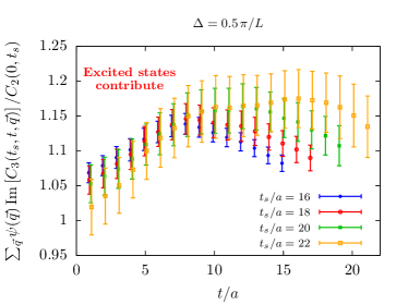
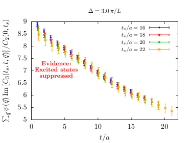
Figure 1 displays the first results for two different spatial localizations $\Delta=0.5\pi/L$ and $\Delta=3\pi/L$. In the left panel, a trend of wโ€‹(ฮ”,t,ts)๐‘คฮ”๐‘กsubscript๐‘ก๐‘ w(\Delta,t,t_{s}) as a function of tssubscript๐‘ก๐‘ t_{s} is seen. For the stronger localization, wโ€‹(ฮ”,t,ts)๐‘คฮ”๐‘กsubscript๐‘ก๐‘ w(\Delta,t,t_{s}) is independent of tssubscript๐‘ก๐‘ t_{s} for $t\gtrsim 0.4\,$fm, within the statistical uncertainty.

Refer to caption
Refer to caption
Figure 1: The observable wโ€‹(ฮ”,t,ts)๐‘คฮ”๐‘กsubscript๐‘ก๐‘ w(\Delta,t,t_{s}) on ensemble D200, as a function of the current insertion time $t$ for two different momentum-space widths $\Delta\in\{1/2,3\}\pi/L$ of the wave packet.

In Figure 2 we show the results of correlated two-parameter fits for the axial charge $g_{A}$ and the axial mass $M_{A}$ for $\Delta\in\{3/2,5/2\}\pi/L$. We used six time slices for the fits $t\in[9,14]\,a$. In the case displayed in the left panel, the fit has no sensitivity to $M_{A}$, because the wave packet suppresses large-momentum contributions. For stronger localizations (right panel), we are sensitive to both parameters.

Refer to caption
Refer to caption
Figure 2: Correlated two-parameter fits to the lattice data for the parameters $(g_{A},M_{A})$, using the ground-state contribution to wโ€‹(ฮ”,t,ts)๐‘คฮ”๐‘กsubscript๐‘ก๐‘ w(\Delta,t,t_{s}) given in Eq.ย (2.13), for $\Delta=1.5\pi/L$ (left) and $\Delta=2.5\pi/L$ (right).

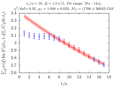
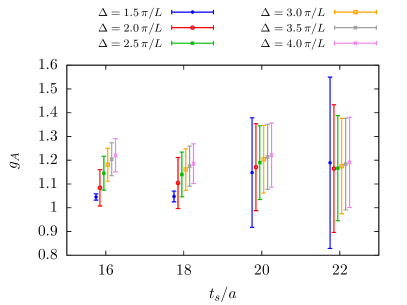
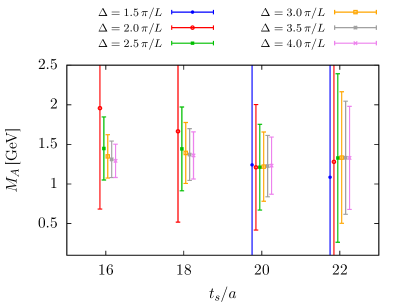
Figure 3 shows the fit results for different sizes $\Delta$ of localizations. The smaller source-sink separations show smaller statistical errors but a larger sensitivity of $g_{A}$ to the width of the wave packet. The results for $g_{A}$ are compatible with the result ($g_{A}=1.188\pm 0.025$) obtained from a different method, namely simultaneous fits to nucleon three-point functions at $\vec{q}=0$ with different currentsย [11], but have a larger statistical error, as they are obtained from a small number of data.

4 Summary and Conclusions

We investigated a new method to compute nucleon form factors in lattice QCD based on spatially localizing the current with a Gaussian profile. We found evidence that for the transverse matrix elements of the axial current, excited states get additionally suppressed as the localization becomes stronger in position space, even though the dispersion relation of $G_{A}$ starts with a three-pion continuum. From the discussion around Eq.ย (5), we expect that for form factors whose dispersive representation starts with a two-pion cut (e.g.ย isovector vector or scalar isoscalar form factors), the excited-state contamination due to spatially distant contributions should be relatively more important, and it must be very large when the pion pole contributes. We were able to extract the axial charge and dipole-mass from fits to lattice data with a localized axial current in the plane transverse to the nucleon spin. In the near future, we will perform fits to several source-sink separations simultaneously, and apply the method to the extraction of $G_{P}$. Also, to better constrain the $Q^{2}$ dependence of the form factor, one could use as a set of wave packets the Hermite polynomials times a Gaussian of fixed width.

Refer to caption
Refer to caption
Figure 3: Summary of fit results for the axial charge (left) and the axial mass (right) for different momentum-space widths $\Delta$ of the wave packet.

Acknowledgements: This project is supported by the DFG via the CRCโ€‰1044 and by the European Research Council (ERC) under the European Unionโ€™s Horizon 2020 research and innovation programme through grant agreement 771971-SIMDAMA. The data has been produced on the HPC cluster โ€Cloverโ€ at the Helmholtz-Institute Mainz. The D200 ensemble was produced on JUQUEEN using computing time provided by the Gauss Centre for Supercomputing through the John von Neumann Institute for Computing.

References

  • [1] V.ย Bernard, L.ย Elouadrhiri and U.-G. MeiรŸner, Axial structure of the nucleon, Journal of Physics G Nuclear Physics 28 (2002) R1 [hep-ph/0107088].
  • [2] J.ย Green, Systematics in nucleon matrix element calculations, in 36th International Symposium on Lattice Field Theory (Lattice 2018) East Lansing, MI, United States, July 22-28, 2018, 2018.
  • [3] O.ย Bรคr, Nucleon-pion-state contamination in lattice calculations of the axial form factors of the nucleon, in 36th International Symposium on Lattice Field Theory (Lattice 2018) East Lansing, MI, United States, July 22-28, 2018, 2018, 1808.08738.
  • [4] K.-F. Liu, J.ย Liang and Y.-B. Yang, Variance Reduction and Cluster Decomposition, Phys. Rev. D97 (2018) 034507 [1705.06358].
  • [5] H.ย B. Meyer, Lorentz-covariant coordinate-space representation of the leading hadronic contribution to the anomalous magnetic moment of the muon, Eur. Phys. J. C77 (2017) 616 [1706.01139].
  • [6] M.ย Bruno, D.ย Djukanovic, G.ย P. Engel, A.ย Francis, G.ย Herdoiza, H.ย Horch etย al., Simulation of QCD with N f = 2 + 1 flavors of non-perturbatively improved Wilson fermions, Journal of High Energy Physics 2 (2015) 43 [1411.3982].
  • [7] M.ย Lรผscher and S.ย Schaefer, Lattice QCD without topology barriers, Journal of High Energy Physics 7 (2011) 36 [1105.4749].
  • [8] M.ย Bruno, T.ย Korzec and S.ย Schaefer, Setting the scale for the CLS $2+1$ flavor ensembles, Phys. Rev. D95 (2017) 074504 [1608.08900].
  • [9] G.ย S. Bali, S.ย Collins and A.ย Schaefer, Effective noise reduction techniques for disconnected loops in lattice qcd, Computer Physics Communications 181 (2010) 1570 .
  • [10] T.ย Blum, T.ย Izubuchi and E.ย Shintani, New class of variance-reduction techniques using lattice symmetries, Phys. Rev. D88 (2013) 094503 [1208.4349].
  • [11] K.ย Ottnad, T.ย Harris, H.ย Meyer, G.ย von Hippel, J.ย Wilhelm and H.ย Wittig, Nucleon charges and quark momentum fraction with $N_{f}=2+1$ Wilson fermions, ArXiv e-prints (2018) [1809.10638].