How reactant polarization can be used to change the effect of interference on reactive collisions

Abstract

It is common knowledge that integral and differential cross sections (DCSs) are strongly dependent on the spatial distribution of the molecular axis of the reactants. Hence, by controlling the axis distribution, it is possible to either promote or hinder the yield of products into specific final states or scattering angles. This idea has been successfully implemented in experiments by polarizing the internuclear axis before the reaction takes place, either by manipulating the rotational angular distribution or by Stark effect in the presence of an orienting field. When there is a dominant reaction mechanism, characterized by a set of impact parameters and angles of attack, it is expected that a preparation that helps the system to reach the transition state associated with that mechanism will promote the reaction, whilst a different preparation would generally impair the reaction. However, when two or more competing mechanisms via interference contribute to the reaction into specific scattering angles and final states, it is not evident which would be the effect of changing the axis preparation. To address this problem, throughout this article we have simulated the effect that different experimental preparations have on the DCSs for the H + D₂ reaction at relatively high energies, for which it has been shown that several competing mechanisms give rise to interference that shapes the DCS. To this aim, we have extended the formulation of the polarization dependent DCS to calculate polarization dependent generalized deflection functions of ranks greater than zero. Our results show that interference are very sensitive to changes in the internuclear axis preparation, and that the shape of the DCS can be controlled exquisitely.

I Introduction

One of the main goals of reaction dynamics is to provide tools that permits the control of the outcome of a chemical event. Bernstein et al. (1987) Ideally, one would wish to set up an experiment where only the desired product (in the desired internal state) will be produced. To achieve that task, one should be able to imagine an experiment where the relative geometry and energy of the incoming atoms can be selected in such a way that maximizes the cross-section of the specific reaction whilst minimizing it for any other side-reaction. To prepare such experiment, it would be necessary a complete knowledge of all the competing dynamical mechanisms.

For reactions taking place in solution, the most it can be done is to choose the temperature, the solvent and the catalyzers that would promote the reaction. For bimolecular reactions in gas phase, however, it is possible to carry out sophisticated experiments selecting, with extremely high resolution, the relative energy, the initial quantum state, and to detect the products with angular resolution. Moreover, it is possible to polarize the reactants bond-axis or rotational angular momentum, so it can be achieved some control into the relative geometry of the reactants before their interactions. For the non-familiar reader that may sound utopia, but several groups have succeeded in carrying out such experiments using either optical alignment methods,Weida and Parmenter (1997); Wang et al. (2011, 2012); Wang and Liu (2016, 2016); Lorenz et al. (2001); Brouard et al. (2015); Chadwick et al. (2014); Brouard et al. (2013); Kandel et al. (2000); Mukherjee and Zare (2010, 2011); Perreault et al. (2017, 2018); Sharples et al. (2018) brute force through intense laser fields Loesch and Möller (1992); Loesch (1995); Loesch and Möller (1998); Kim and Felker (1996); Sakai et al. (1999); Rosca-Pruna and Vrakking (2001); Stapelfeldt and Seideman (2003); Hamilton et al. (2005); Holmegaard et al. (2009); Ghafur et al. (2009); Friedrich and Herschbach (1991, 1999), or using static orienting fields in tandem with hexapole state selection.Parker and Bernstein (1989); Aoiz et al. (2015); de Lange et al. (2004, 1999); van Beek et al. (2000); Vogels et al. (2018); Onvlee et al. (2017)

Based on the experimental set-up by Kandel et al.,Kandel et al. (2000) in a series of articles we have suggested a hypothetic crossed-beam experiment for atom-diatom reactions where the diatom (in this case D₂) is prepared in a $|v=0,j=2,m=0\rangle$ state, where $v$, $j$, and $m$ are the vibrational, rotational and magnetic quantum number.Aldegunde et al. (2005) The latter is determined with regard to a laboratory-fixed (space-fixed) quantization axis (usually the light polarization vector or the direction of light propagation for circularly polarized light). For a $m$=0 state, the internuclear axis is preferably aligned along the quantization axis (a directed state).Kais and Levine (1987) The direction of the laboratory-fixed axis with regard to the scattering frame – defined by the initial relative velocity, $\bm{k}$, and the plane containing $\bm{k}$ and $\bm{k}^{\prime}$, the final relative velocity – can be chosen arbitrarily, allowing us to select the relative geometry of the incoming reactants.

Although the aforementioned experiments are indeed challenging, the idea behind them it is rather simple. The transition states have a well defined geometry; therefore, if we select a configuration that aids the reactants to reach the transition state, larger cross sections will be achieved, whilst if that configuration does not lead to the neighborhoods of the transition state, reaction will be impaired. However, that simple idea may not be valid when quantum interference effects play an important role, and something apparently as simple as a reaction mechanism is not so clearly defined. For example, for the reactive collisions between H and D₂ at high collision energies Jambrina et al. (2015, 2016); Sneha et al. (2016); Aoiz and Zare (2018) and certain final rovibrational states, the angular distribution showed prominent peaks and dips that are the result of quantum interference between the classical mechanisms previously described by Wrede and coworkers,Greaves et al. (2008, 2008) one preferring collinear collisions with a linear intermediate collision complex (denoted to as the spiral in ref. 42), whilst the other correlates with T-shape as intermediate triatomic arrangement (denoted in ref. 42 as the ear).

If these mechanisms do not interfere, by selecting the geometry of the incoming reagents, it would be possible to promote any of them. However, as long as they do, it does not become easy to predict what would be the outcome of the collision upon selection of the incoming geometry of the reactants. Throughout this article, we will tackle this problem and we will show that an exquisite control of the position and intensity of the peaks of the differential cross section (DCS) can be achieved by varying the polarization of the reactants before the collision.

The article is organized as follows: In Section II we review the main quantum mechanical (QM) expressions for the calculation of the observable DCS for a given reactants preparation. Next, (Section II.3) we extend the formulation to the treatment of Polarization Dependent Quantum Generalized Deflection Functions that will be used to aid to the interpretation of the main features of the observable DCSs. The results and their discussion are presented in Section III. Finally, the main conclusions of the article are highlighted in Section 4.

II Theory

II.1 Polarization Dependent Differential Cross Sections

The polarization dependent differential cross sections (PDDCSs) are the polarization moments that describe either the distribution of the initial angular momentum vector (and, consequently, of molecular axes) that give rise to the reaction at a given scattering angle into a final state, or the distribution of the rotational angular momentum resulting from a reaction into a scattering angle. These magnitudes, their expressions and physical meanings have been discussed at length in previous publications Shafer et al. (1995); Aoiz et al. (1996); de Miranda et al. (1999); Aldegunde et al. (2005, 2008) and the reader is referred to them for a thorough explanation. In the present context, we will consider the former; that is, the PDDCSs associated with the ${\bm{k}}-{\bm{j}}-{\bm{k}^{\prime}}$ correlation, also known as reactant $j$-PDDCSs, which, for a given state-to-state process, provide information about the preferred direction of the rotational diatomic angular momentum ($\bm{j}$) of the incoming molecule to give rise to reaction into a specific final state.

The PDDCSs are intrinsic magnitudes, hence pure dynamical properties that reflect the anisotropy of the potential and whose values will depend on the steric requirements of the studied process. Therefore, intrinsic polarization moments are inherent to the collision process and are independent of external circumstances (the experimental setup). Accordingly, they can be directly extracted from the Scattering matrix.

The expression that relates the unnormalized PDDCSs with the elements of the scattering matrix is:

$$U^{(k)}_{q}(\theta) = \frac{1}{2j+1}\sum_{\Omega^{\prime}}\sum_{\Omega_{1}\Omega_{2}}f_{v^{\prime},j^{\prime},\Omega^{\prime}~{}v,j,\Omega_{1}}(\theta)\times$$ (1)

$$f^{*}_{v^{\prime},j^{\prime},\Omega^{\prime}~{}v,j,\Omega_{2}}(\theta)\langle j,\Omega_{1},kq|j\Omega_{2}\rangle$$

where $\theta$ is the scattering angle (that between $\bm{k}$ and $\bm{k}^{\prime}$), $U^{(k)}_{q}(\theta)$ denotes the unnormalized $j$-PDDCS of rank $k$ and component $q$, $\langle j,\Omega_{1},kq|j\Omega_{2}\rangle$ is the Clebsch-Gordan coefficient, and $f_{v^{\prime},j^{\prime},\Omega^{\prime}~{}v,j,\Omega}(\theta)$ is the scattering amplitude for the state-to-state, $v,j,\Omega\to v^{\prime},j^{\prime},\Omega^{\prime}$, process. [In previous works,Kandel et al. (2000); Aldegunde et al. (2005, 2008) we have used the normalized PDDCS, $S^{(k)}_{q}(\theta)=(2\pi/\sigma_{\rm iso})\,U^{(k)}_{q}(\theta)$, where $\sigma_{\rm iso}$ is the integral cross section in the absence of angular momentum polarization.]

The scattering amplitude can be written in terms of the Scattering matrix elements, ${\textsf{S}}^{J}_{v^{\prime},j^{\prime},\Omega^{\prime}v,j,\Omega}$, as

$$f_{v^{\prime},j^{\prime},\Omega^{\prime}v,j,\Omega}(\theta)=\frac{1}{2i\,k_{\rm in}}\sum_{J}\,(2J+1)d^{J}_{\Omega^{\prime}\Omega}(\theta){\textsf{S}}^{J}_{v^{\prime},j^{\prime},\Omega^{\prime}v,j,\Omega}\,,$$ (2)

where $k_{\rm in}$ is the reactant’s wave-number and $d^{J}_{\Omega^{\prime}\Omega}(\theta)$ is the reduced Wigner-rotation matrix. In what follows, to simplify the notation, we will write $f_{\Omega^{\prime}\Omega}(\theta)$, implying definite values of initial $v$, $j$ and final $v^{\prime}$, $j^{\prime}$ states.

Each $U^{(k)}_{q}(\theta)$, $k\in[0,2j]$ $q\in[-k,k]$, provides different physical and “directional” information about the polarization of the rotational angular momentum.de Miranda et al. (1999) Even $k$ moments are associated with alignment and odd $k$ moments with orientation. When $k$=0, the corresponding PDDCS, $U^{(0)}_{0}(\theta)$, is nothing but the unpolarized (or isotropic) DCS.

II.2 Observable Differential Cross Section

The counterpart of the intrinsic polarization moments are the extrinsic polarization moments, $A^{(k)}_{q}$, that provide information about the preparation of the reactant rotational angular momentum; that is, about the various possible experimental schemes for orienting or aligning reactant molecules.Aldegunde et al. (2005)

Whilst the intrinsic PDDCSs inform us about the steric preference of the reactions (what the reaction “wants”), the extrinsic polarization moments tell us about the rotational angular momentum and molecular bond axis distributions in the asymptotic region, prior to any interaction between the reactants (what we experimentally “offer” to the reaction). As such, extrinsic polarization moments are a consequence of external circumstances (the experimental setup) rather than the reaction itself.

Hence, it is evident that the DCS that can be measured for a given experimental preparation of the rotational angular momentum (hereinafter observable DCS) will be a combination of both extrinsic and intrinsic polarizations. Of course, in the absence of external reactant polarization, the measurement would yield the conventional, unpolarized or isotropic DCS, which quantifies the two-vector $\bm{k}-\bm{k^{\prime}}$ correlation. The expression that relates the observable DCS to both types of moments is:Aldegunde et al. (2005, 2011)

$$\frac{d\sigma_{\alpha}^{\beta}}{d\omega}\equiv{\rm d}\sigma(\theta|\beta,\alpha) = \sum_{k}\sum_{q=-k}^{k}(2k+1)\left[U^{(k)}_{q}(\theta)\right]^{*}\times$$ (3)

$$A^{(k)}_{0}C_{kq}(\beta,\alpha)$$

This expression contains the products of extrinsic and intrinsic polarization moments of the same rank. Apart from these moments, eqn (3) includes the modified spherical harmonics, $C_{kq}(\beta,\alpha)$, needed to rotate the extrinsic moments $A^{(k)}_{q}$, defined in the laboratory frame, to the scattering frame where the $U^{(k)}_{q}(\theta)$ are defined. The Euler angles that connect both the laboratory and the scattering frame are $\beta$ (polar), and $\alpha$ (azimuthal). Therefore, the observable DCS depends on those angles; i. e., for a given extrinsic preparation, it depends on the angles that define the laboratory with respect to the scattering frame. These angles can be varied experimentally (for instance, changing the light polarization vector with respect to the relative velocity) giving rise to different preparations of the angular momentum.

As an example, a possible preparation for the D₂ molecule in $v$=0 (whose reaction with H atoms will be considered in this work) could be to select $|j=2,m=0\rangle$ state, which is a directed state.Kais and Levine (1987) This can be achieved by pure rotational Raman scattering by selecting the right pump and Stokes laser frequencies for stimulated Raman scattering. By excitation via the $S(0)$ transition from D₂($v=0,j=0$), a considerable excitation to D₂($v=0,j=2$) can be produced quite effectively by setting the polarizations of the stimulated Raman pump and Stokes lasers parallel to each other.Kandel et al. (2000); Mukherjee and Zare (2010, 2011)

In that case, the only non-vanishing polarization parameters, $A^{(k)}_{q}$, in the laboratory frame are:

$$A^{(0)}_{0}=1, \quad A^{(2)}_{0}=\langle 20,20|20\rangle=-\sqrt{\frac{2}{7}},$$ (4)

$$A^{(4)}_{0}=\langle 20,40|20\rangle=\sqrt{\frac{2}{7}}$$

Varying the $\beta$ and $\alpha$ angles, the prepared state can be directed at any arbitrary direction in the scattering frame.

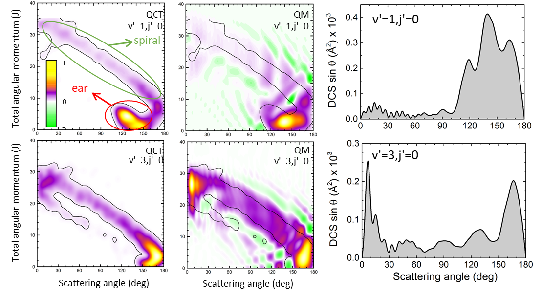
Figure 1: Comparison of the QCT (left panels) and QM (middle panels) generalized deflection functions (GDF) for the H +D${}_{2}(v=0,j=2)\rightarrow$ HD($v^{\prime}$,$j^{\prime}=0$) + D reaction ($v^{\prime}$=1 upper panels, $v^{\prime}$=3 bottom panels) at $E_{\rm col}=$1.97 eV. The contour of the QCT deflection function has been added to the QM $Q_{r}$ to make the comparison easier. The green contours corresponds to destructive interferences ($Q_{r}<0$). The QM DCSs for both reaction channels are shown in the right panels.

II.3 Polarization Dependent Generalized Deflection Functions

The quantum deflection function is the functional of the deflection angle in terms of the angular momentum $J$. It is a valuable magnitude to get some additional insight into a scattering process, in particular to predict the presence of rainbows and interference between near-side and far-side encounters.Connor (2004); Xiahou and Connor (2009); Shan and Connor (2011) As an extension, we have recently derived a Generalized Deflection Function (GDF),Jambrina et al. (2018) that can be considered as the joint probability (quasi-probability in the QM case) density function of $J$ and $\theta$. This formulations allows us to plot a $J-\theta$ map that can be used to distinguish between different reaction mechanisms, and to discern interference between them. The reader is referred to Ref. 52 for a detailed discussion.

In this article we extend the GDF formulation to deal with polarized reactants. We start this section by summarizing the main expressions needed to calculate QM GDFs that can be easily implemented in any QM scattering code. First of all, we define the $J$-partial dependent scattering amplitude as:

$$f^{J}_{\Omega^{\prime}\Omega}(\theta)=\frac{1}{2i\,k_{\rm in}}\,(2J+1)d^{J}_{\Omega^{\prime}\Omega}(\theta){\textsf{S}}^{J}_{\Omega^{\prime}\Omega}$$ (5)

where $\Omega$ and $\Omega^{\prime}$ are bounded within $[-J,+J]$. The (summed over $J$) scattering amplitude can now be written as:

$$f_{\Omega^{\prime}\Omega}(\theta)=\sum_{J=0}^{J_{\max}}f^{J}_{\Omega^{\prime}\Omega}(\theta)\,,$$ (6)

where $J_{\max}$ is the maximum total angular momentum leading to reaction. The DCS (that is, the $U^{(0)}_{0}(\theta)$ PDDCS) in the absence of reagent’s polarization (i.e., isotropic preparation) can be expressed as a function of the $J$-partial scattering amplitudes:

$${\rm d}\sigma_{r}(\theta|{\rm iso})=\frac{1}{2j+1}\,\sum_{\Omega^{\prime}}\sum_{\Omega}~{}\,\sum_{J_{1}=0}^{J_{\max}}\sum_{J_{2}=0}^{J_{\max}}f^{J_{1}}_{\Omega^{\prime}\Omega}(\theta)f^{J_{2}*}_{\Omega^{\prime}\Omega}(\theta)\,,$$ (7)

which can also be written as:Jambrina et al. (2018)

$${\rm d}\sigma_{r}(\theta|{\rm iso}) = \frac{1}{2j+1}\,\sum_{\Omega^{\prime}}\sum_{\Omega}~{}\sum_{J=0}^{J_{\max}}\,\sum_{J_{1}=0}^{J_{\max}}\sum_{J_{2}=0}^{J_{\max}}\frac{\left(\delta_{J_{1},J}+\delta_{J_{2},J}\right)}{2}\,\times$$ (8)

$$f^{J_{1}}_{\Omega^{\prime}\Omega}(\theta)f^{J_{2}*}_{\Omega^{\prime}\Omega}(\theta).$$

In a similar way, it is possible to express the PDDCSs as a function of the $f^{J}_{\Omega^{\prime}\Omega}$,

$$U^{(k)}_{q}(\theta) = \frac{1}{2j+1}\sum_{\Omega^{\prime}}~{}\,\sum_{J_{1}=0}^{J_{\max}}\sum_{J_{2}=0}^{J_{\max}}\sum_{\Omega_{1}}\sum_{\Omega_{2}}f^{J_{1}}_{\Omega^{\prime}\Omega_{1}}(\theta)f^{J_{2}*}_{\Omega^{\prime}\Omega_{2}}(\theta)\times$$ (9)

$$\langle j\Omega_{1},kq|j\Omega_{2}\rangle\,,$$

By invoking the triangular relationship of the Clebsch-Gordan coefficients, eqn. (9) can be simplified to:

$$U^{(k)}_{q}(\theta) = \!\!\frac{1}{2j+1}\sum_{\Omega^{\prime}}~{}\sum_{J_{1}=0}^{J_{\max}}\sum_{J_{2}=0}^{J_{\max}}\sum_{\Omega}f^{J_{1}}_{\Omega^{\prime}\Omega}(\theta)f^{J_{2}*}_{\Omega^{\prime}\Omega+q}(\theta)\times$$ (10)

$$\langle j\Omega,kq|j\Omega+q\rangle\,,$$

and, similarly to eqn (8), eqn (9) can be recast as

$$U^{(k)}_{q}(\theta) = \frac{1}{2j+1}\sum_{\Omega^{\prime}}~{}\sum_{J=0}^{J_{\max}}\sum_{J_{1}=0}^{J_{\max}}\sum_{J_{2}=0}^{J_{\max}}\sum_{\Omega}\frac{\left(\delta_{J_{1},J}+\delta_{J_{2},J}\right)}{2}\,\times$$ (11)

$$f^{J_{1}}_{\Omega^{\prime}\Omega}(\theta)f^{J_{2}*}_{\Omega^{\prime}\Omega+q}(\theta)\langle j\Omega,kq|j\Omega+q\rangle\,.$$

In a previous work,Jambrina et al. (2018) it was shown that it is possible to define a quantum analog of the classical joint probability distribution of the scattering angle and the total angular momentum, that can be written as:

$$Q_{r}(\theta,J) = \frac{\sin\theta}{2j+1}\,\sum_{\Omega^{\prime}\Omega}~{}\sum_{J_{1}=0}^{J_{\max}}\sum_{J_{2}=0}^{J_{\max}}\,\frac{\left(\delta_{J_{1},J}+\delta_{J_{2},J}\right)}{2}\times$$ (12)

$$f^{J_{1}}_{\Omega^{\prime}\Omega}(\theta)f^{J_{2}*}_{\Omega^{\prime}\Omega}(\theta)\,.$$

Unlike the classical GDF and the classical or quantal DCSs, the QM GDF, $Q_{r}(\theta,J)$, can take positive or negative values. Also, in contrast to the DCS, the QM GDFs are additive with respect to the contribution of $J$ partial waves:

$$\sum_{J=J_{1}}^{J_{2}}Q_{r}(\theta,J)+\sum_{J=J_{2}}^{J_{3}}Q_{r}(\theta,J)=\sum_{J=J_{1}}^{J_{3}}Q_{r}(\theta,J)\,,$$ (13)

with $J_{1}<J_{2}<J_{3}$. Additionally, the QM GDF complies with the following relationships:

$$\displaystyle{\sum_{J=0}^{J_{\max}}}Q_{r}(\theta,J)={\rm d}\sigma_{r}(\theta|{\rm iso})\sin\theta$$ (14)

$$\displaystyle\int_{0}^{\pi}\int_{0}^{2\pi}Q_{r}(\theta,J){\rm d}\theta{\rm d}\phi=\frac{\pi}{k^{2}_{\rm in}}\,(2J+1)P_{r}(J)=\sigma^{J}_{r}$$ (15)

$$\displaystyle\sum_{J=0}^{J_{\max}}~{}\int_{0}^{\pi}Q_{r}(\theta,J){\rm d}\theta{\rm d}\phi=\sigma_{\rm iso}$$ (16)

where $P_{r}(J)$ is the reaction probability as a function of the total angular momentum. It is related to the $J$-partial cross section by $\sigma^{J}_{r}=\pi/k^{2}_{\rm in}\,(2J+1)P_{r}(J)$.

Following the same procedure as that used to derive the QM GDF, higher-rank GDFs can be defined as:

$$Q^{(k)}_{q}(\theta,J)= \displaystyle{\frac{\sin\theta}{2j+1}}\,\sum_{\Omega^{\prime}}~{}\sum_{J_{1}=0}^{J_{\max}}\sum_{J_{2}=0}^{J_{\max}}\,\sum_{\Omega}\,\frac{\left(\delta_{J_{1},J}+\delta_{J_{2},J}\right)}{2}\,\,$$ (17)

$$f^{J_{1}}_{\Omega^{\prime}\Omega}(\theta)f^{J_{2}*}_{\Omega^{\prime}\Omega+q}(\theta)\,\langle j\Omega,kq|j\Omega+q\rangle\,.$$

where $Q^{(k)}_{q}(\theta,J)$ denotes the GDF with rank $k$ and component $q$.

For $q$=0 moments, the only differences between eqn (17) and (12) is the presence of the Clebsch-Gordan coefficient. In particular, for $k$=0 eqn (12) is recovered. Furthermore, integration of $Q^{(k)}_{q=0}(\theta,J)$ over $\theta$ allows us to recover the $J$-dependent polarization parameters.Aldegunde et al. (2012) For $q\neq 0$, eqn (17) involves the product of $J$-partial dependent scattering amplitude of different $\Omega$ values and no simple analytical formula can be derived, although numerical integration leads to the $J$-dependent polarization parameters, $P^{(k)}_{q}(J)$. Finally, regardless of the value of $q$, summation of eqn (17) over $J$ retrieves the $U^{(k)}_{q}(\theta)\,\sin\theta$.

It is a common practice in stereodynamics to define renormalized PDDCSs, independent of the flux at each scattering angle, and whose limits are well defined.Aldegunde et al. (2008) In principle, the same normalization could be applied to the the $Q^{(k)}_{q}(\theta,J)$. However, because GDFs can take positive or negative values (that could even canceled out for a certain range of $J$s), renormalized $Q^{(k)}_{q}(\theta,J)$ have no definitive limits and its use is not practical.

In analogy with the definition of the observable DCS, eqn (3), the $Q^{(k)}_{q}(\theta,J)$ can be combined to calculate $Q^{\beta}_{\alpha}(\theta,J)$, i.e., QM GDFs that depend on the experimental preparation of the reactants and whose sum over $J$ yields the observable DCS. The expression for the calculation of $Q^{\beta}_{\alpha}(\theta,J)$ is

$$Q^{\beta}_{\alpha}(\theta,J)=\frac{\sigma_{\rm iso}}{2\pi}\sum_{k}\sum_{q=-k}^{k}(2k+1)\left[Q^{(k)}_{q}(\theta,J)\right]^{*}A^{(k)}_{q}C_{kq}(\beta,\alpha)$$ (18)

We will make extensive use of this equation to determine the QM GDFs under different preparation of the angular momentum direction.

III Results and Discussion

Figure 2: Differential Cross Sections for the H+D${}_{2}($v$=0,$j$=2\rightarrow$HD($v^{\prime}$=1,$j^{\prime}=0$)+D reaction at $E_{\rm col}=$1.97 eV for $\beta$=0. The isotropic DCS is shown in gray and the observable DCS in red. The extrinsic preparation of the internuclear axis of D₂ referred to the scattering frame is shown in an inset. The QM GDFs for the polarized reactants is shown in the bottom panel.

We will start this section with the discussion of the shape of the isotropic QM DCSs and its connection with the quasiclassical deflection functions (QCT GDF); that is, the joint probability density function of $\theta$ and $J$. These results have been presented previouslyJambrina et al. (2015, 2016) and are repeated here for completeness and to link up with the subsequent discussion. The interested reader is referred to Ref. 38; 39 for a thorough discussion.

The DCSs for the H + D₂($v$=0,$j$=2) $\rightarrow$ D + HD($v^{\prime}$,$j^{\prime}$) reaction at E_col=1.97 eV are shown in the right panels of Fig. 1. For $v^{\prime}$=1, $j^{\prime}$=0, (upper panel) the products are mainly scattered in the backward hemisphere where three peaks are observed, one peak at 150^∘, and two smoother peaks at 120^∘ and 175^∘. These peaks were also present in the DCSs of the reactions of H with D₂($v$=0,$j$=0) and with D₂($v$=0,$j$=1).Jambrina et al. (2016) The origin of these structures was attributed to quantum interference between (essentially) two competing classical mechanisms that can be easily elucidated with the help of the QCT DF, which is shown in the left upper panel of Fig. 1. As can be seen, in the backward region, $\theta>$90^∘, there are two separated regions that give rise to products at the same scattering angles. On the one hand, there is scattering from the wide band running diagonally across the $\theta$-$J$ map with a negative slope, that includes all $J$ values contributing to the reaction but the smallest ones ($J\in[0,8]$), region called spiral.Greaves et al. (2008) Although this region covers the whole range of scattering angles, at backward angles the intensity is somewhat larger. On the other hand, scattering in the backward region is mainly caused by another, well separated, confined region, including only small $J$ values (small impact parameters), $J\leq$8, giving rise to products in a limited range, 110-170^∘, of scattering angles, region called ear.Greaves et al. (2008) These two regions in the $\theta$-$J$ map are characterized by distinct classical mechanisms (different impact parameters, angle of attack, intermediate collision complex, etc.) that nevertheless give rise to scattering at the same angles and into the same final states. Therefore, there is small wonder that interference from these separate contributions gives rise to oscillations in the DCS that explain the peak structure observed.

Although the QCT GDFs for different initial $j$ states are remarkably similar,Jambrina et al. (2016) the sharpness of the backward peaks in the DCS was found to decrease with increasing $j$. The reason is not the progressive quenching of interferences with increasing $j$, but rather the incoherent superposition of contributions from different helicity states of the reagents (for $j$=2, $\Omega=0,\pm 1,\pm 2$). As a matter of fact, the decomposition of the QCT GDF into the various $\Omega$ values shows that their respective contributions are associated with different dynamical mechanisms.Jambrina et al. (2016)

The QM GDF, depicted in the middle, upper panel of Fig. 1, has the advantage of allowing the observation of interference between different mechanisms. As can be seen, the spiral mechanism, associated with the diagonal band, is chopped into three pieces, each corresponding to each of three peaks of the DCS. It is worth mentioning that, in a clear contrast to what was observed for the reaction with D₂ in $j$=0,Jambrina et al. (2018) there are no relevant destructive interferences (negative values of $Q_{r}(\theta,J)$, represented as green stripes) between the various groups of $J$ . The lack of negative values precludes the appearance of deep minima as those observed in the DCS for $j$=0 (see Fig. 2 of Ref. 39) and makes the whole structure much smoother.

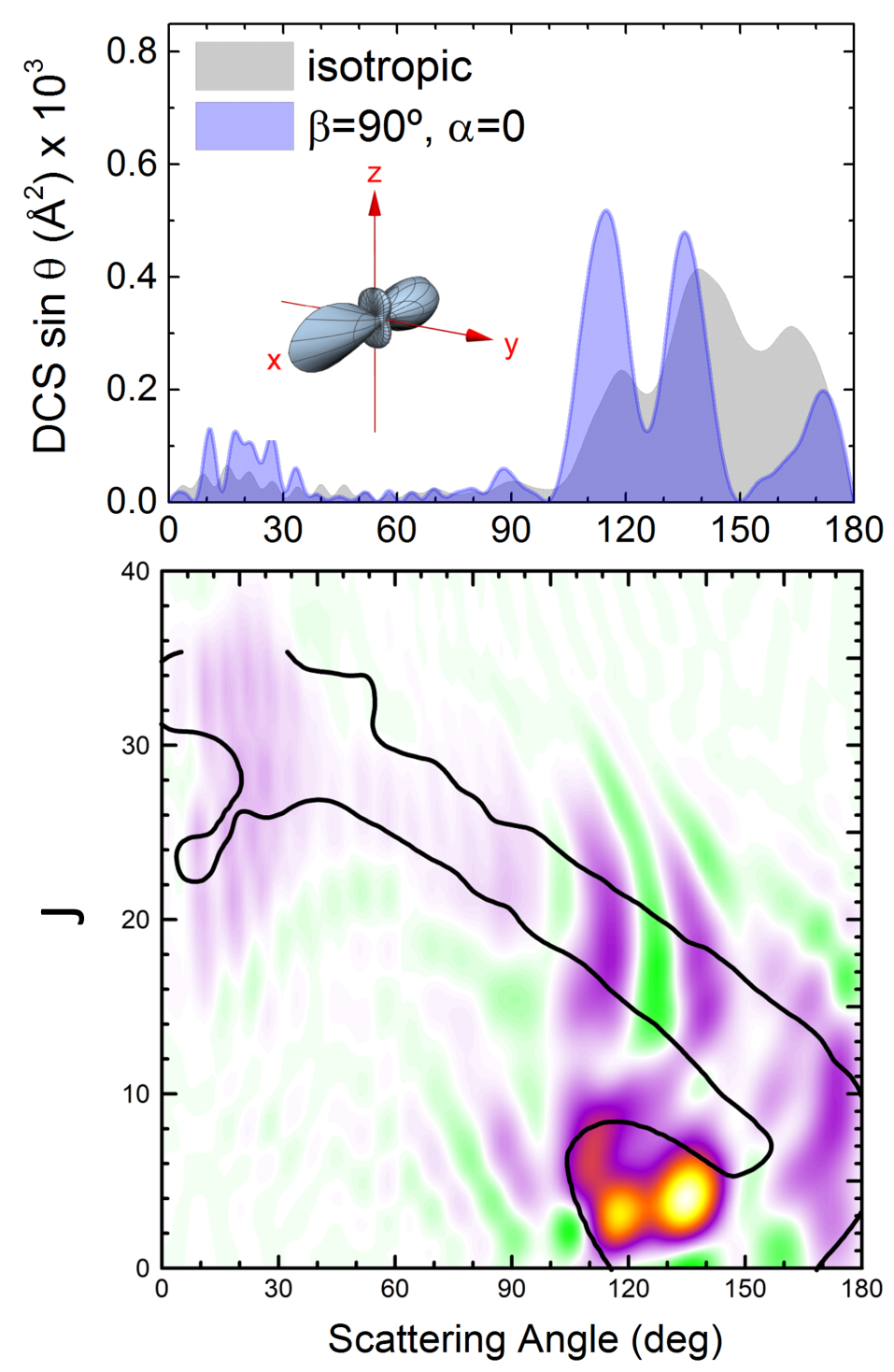
Figure 3: As Fig. 2 but for a $\beta=90^{\circ}$, $\alpha=0$ preparation.

Fig. 1 also contains the respective results for the H + D₂($v$=0,$j$=2) $\rightarrow$ D + HD($v^{\prime}$=3,$j^{\prime}$=0), shown in the lower panels. Although the DCS exhibits several oscillations in the whole range of scattering angles, the observation of the classical and quantal GDFs rules out the presence of strong interference as that observed for $v^{\prime}$=1. Both QCT and QM GDFs are very similar and can be ascribed to the pattern expected for direct reaction with essentially a single mechanism: that corresponding to the spiral, with large (small) angular momenta –or impact parameters– associated with forward (backward) scattering. Moreover, except for some details, the QM GDF for the reaction with D₂ in $j$=0 and in $j$=2 are very much alike.

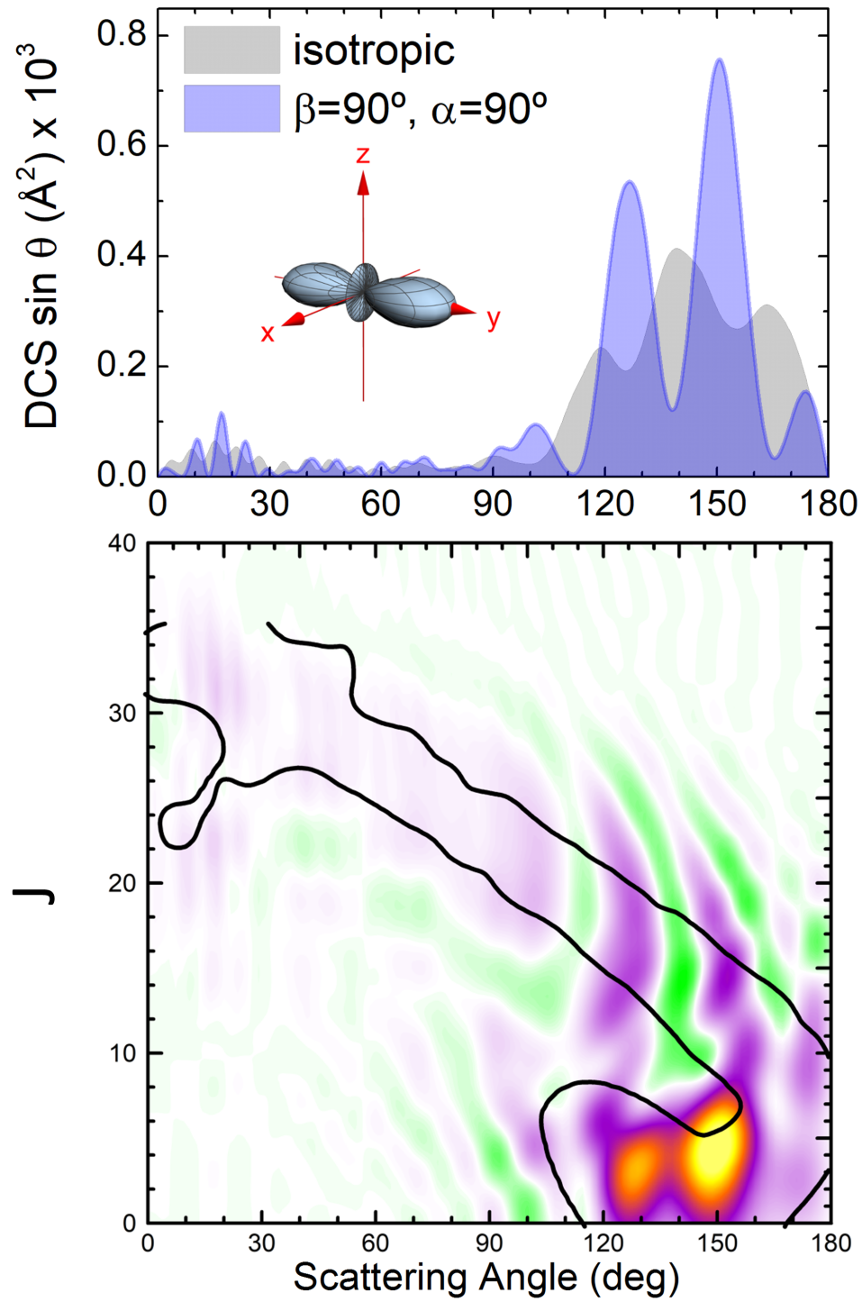
Figure 4: As Fig. 2 but for a $\beta=90^{\circ}$, $\alpha=90^{\circ}$ preparation.

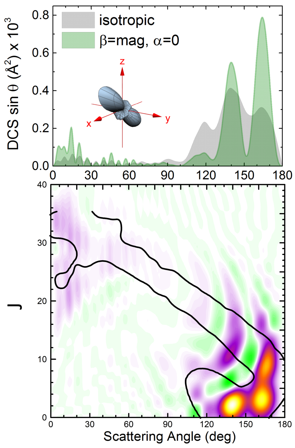
Figure 5: As Fig. 2 but for a $\beta={\rm mag}$, $\alpha=0$ preparation.

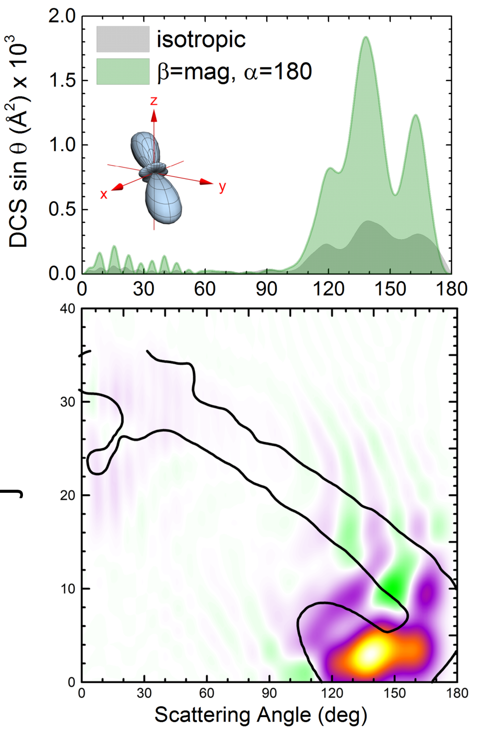
Figure 6: As Fig. 2 but for a $\beta={\rm mag}$, $\alpha=180^{\circ}$ preparation.

So far, we have observed how interference between different mechanisms affects the shape of the DCS for collisions leading to HD($v^{\prime}$=1,$j^{\prime}$=0), for initial $j$=0 and $j$=2. The question that we address in this article is if it would be possible to modulate the effect of this interference by using different polarization of the reactants. Using the analogy with the double-slit experiment, whether we can change not only the intensity, but also the position of the bands and the nodes of probability. To address this question, in the remainder of this article we will present and discuss observable DCSs for different polarizations of the reactants.

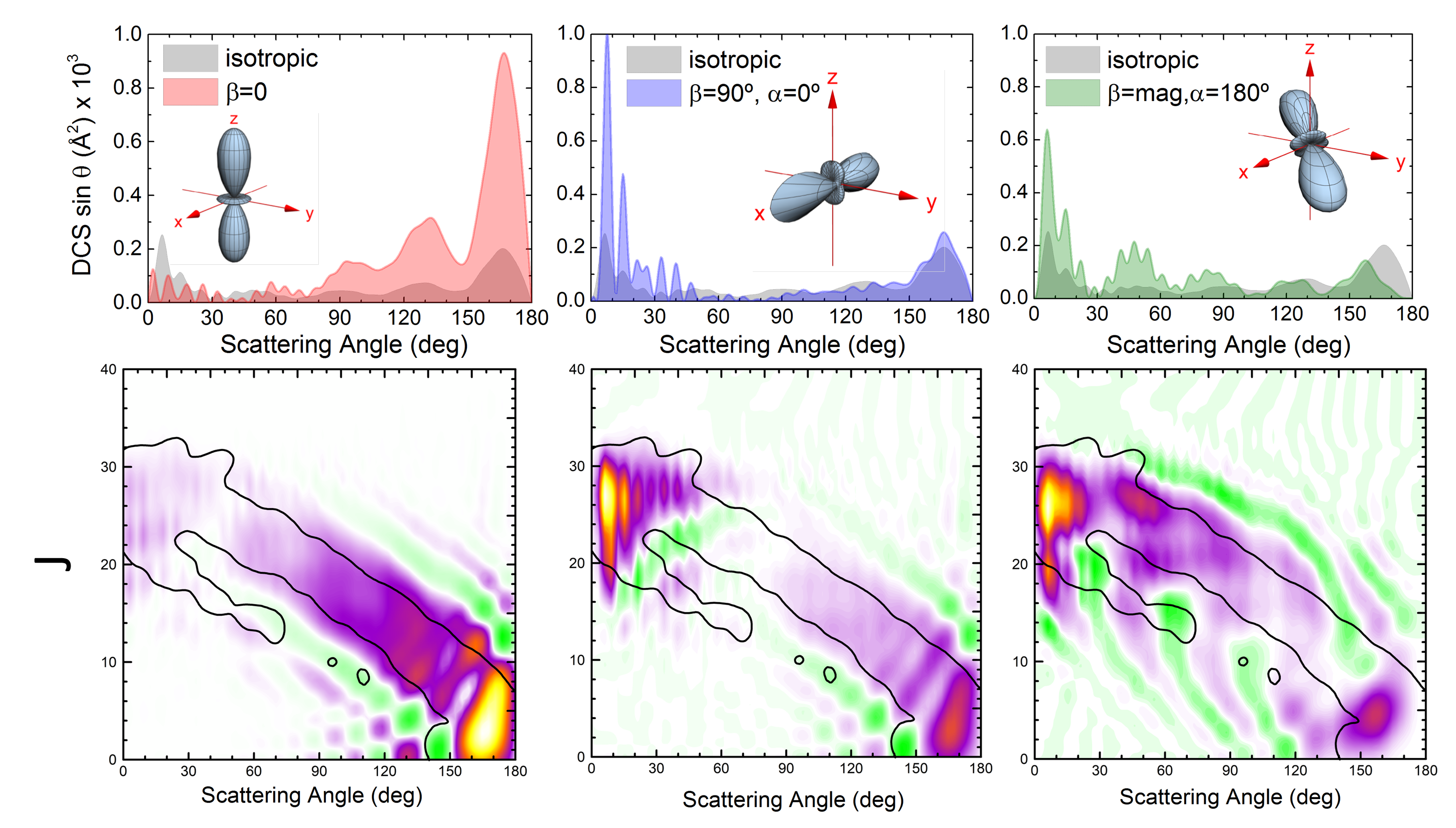
Figure 7: Differential Cross Sections (upper panels) for the H +D${}_{2}($v$=0,$j$=2)$ $\rightarrow$ HD($v^{\prime}$=3,$j^{\prime}=0$) + D reaction at $E_{\rm col}=$1.97 eV for $\beta$=0 (left panel),$\beta=90^{\circ}$, $\alpha=0$ (middle panel), and $\beta={\rm mag}$, $\alpha=180^{\circ}$ (right panel). The isotropic DCS is shown in gray and the observable DCSs are shown in red ($\beta=$0), blue ($\beta=90^{\circ}$), and green ($\beta={\rm mag}$) . The extrinsic preparation of the internuclear axis of D₂ referred to the scattering frame are shown in insets. The corresponding QM GDF for the various polarization schemes are shown in the bottom panels.

Fig. 2 displays the DCS for $\beta$=0, for which the laboratory frame $Z$ axis and the initial relative velocity (scattering frame $z$ axis) are parallel to each other. Under these conditions, D₂ internuclear axis is preferentially along the relative velocity (actually, the DCS for $\beta$=0 is strictly equivalent to that it would be obtained if all scattering would have been caused by $\Omega$=0). Therefore, it can can be expected that this axis preparation would foster the spiral mechanism, that covers the whole range of scattering angles, and it is associated with an essentially collinear transition state. The ${\rm d}\sigma(\theta|\beta=0)$ exhibits three very sharp peaks with deep minima between them. The position of the peaks are only slightly shifted with respect to the peaks found in the isotropic DCS. Based on a QCT analysis,Jambrina et al. (2016) the ear mechanism was assigned to collisions going through a T-shape transition state Greaves et al. (2008, 2008) and, accordingly, it can be expected that this mechanism will be much less important for $\beta$=0. To gain further insight onto the changes observed in the DCS, in the bottom panel of Fig. 2 the QM GDF is depicted. As expected, the relative importance of the spiral mechanism has soared, whilst the ear one has almost disappeared. By inspection of the QM GDF, it can be concluded that the most backward peak is caused by $J$s from 0 to 15, the second peak comes from partial waves up to 20, and the third peak, at 115^∘, is originated by two separate groups of $J$s, one belonging to the spiral and the other from the remnant of the ear mechanism.

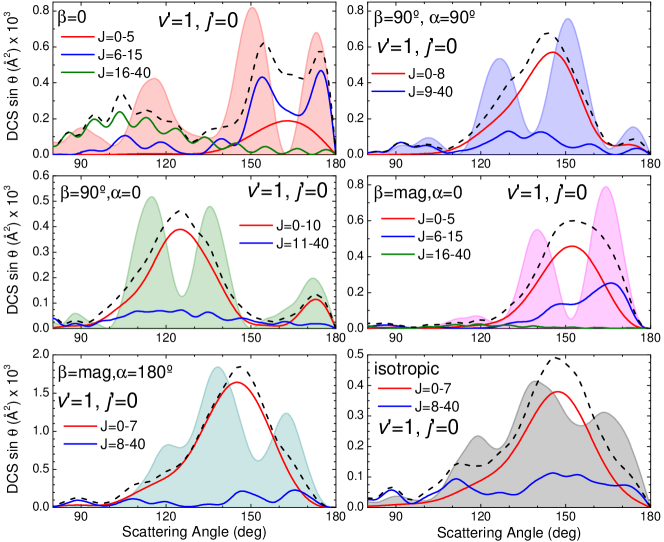
Figure 8: Comparison of the different DCS for the H +D₂ $\rightarrow$ HD($v^{\prime}$=1,$j^{\prime}=0$) + D reaction at $E_{\rm col}=$1.97 eV for different experimental set-up. To illustrate the effect of the interferences in the shape of the DCSs, the contribution of different groups of partial waves have been calculated (see text for further details). The overall DCS is shown shaded and the sum of the contributions of the different groups of $J$s is shown as dashed black lines.

The situation significantly changes when we simulate the observable DCS for $\beta=$90^∘, $\alpha=$0, shown in Fig. 3. This preparation corresponds to side-on, coplanar encounters, with the internuclear axis preferentially along the $x$ direction (on the $\bm{k}$-$\bm{k}^{\prime}$ plane). Again, we can observed three peaks in the DCS somewhat shifted with respect to the much smoother peak of the isotropic DCS. In any case, the relative intensity of those peaks has changed dramatically as compared to isotropic DCS. The peak at 110^∘ is considerably larger and isolated from the second peak by a deep minimum. On the other hand, the most backward peak is considerably less important, and overall the DCS is considerably less backward. The explanation of the main features of the DCS can be extracted from the analysis of the $Q^{90^{\circ}}_{0}(\theta,J)$. As can be observed, in contrast with the $\beta=$0 case, the ear mechanism is strongly favoured and becomes more important than the spiral. The interference between those mechanisms splits the spiral in two sharp peaks at $\approx 110^{\circ}$ and $\approx 140^{\circ}$ that are separated by destructive interference (shown as a green band in the $J-\theta$ map) at 120^∘, which is the position of the dip. Whilst in the isotropic DCS, scattering from the ear and spiral are merged at the most backward region, for DCS($\beta=$90^∘, $\alpha=$0) the ear is confined into a more sideways region leading to a reduction in the backward signal as a results of much less interference with the spiral mechanism.

Intuitively, side-on collisions should be also fostered with a $\beta=$90^∘, $\alpha=$90^∘ axis preparation, and therefore minor changes would be expected when moving from the $\beta=$90^∘, $\alpha=$0 to the $\beta=$90^∘, $\alpha=$90^∘ arrangement. However, as it is shown in Fig. 4, this is not the case. For $\alpha=$90^∘ we observe three peaks, and whilst the intensities of the first and the third peak have barely changed, the second peak is 50 % larger and, hence, is now the most prominent peak. More interestingly, the two most sideways peaks are in anti-phase with the peaks observed for $\alpha=$0. As can be observed in the $Q^{90^{\circ}}_{90^{\circ}}(\theta,J)$, shown in the bottom panel of Fig. 4, those two peaks are caused by interference between the spiral and ear mechanisms, hence proving that the shift in $\alpha$ is enough to change the phase of the interference causing a conspicuous shift in the position of the peaks of the DCS. It is also noticeable that the scattering from the ear mechanism has moved towards backward scattering and splits in two parts by a destructive interference which coincides with the deep minimum observed in the DCS.

Next, we will examine the effects produced with preparations with $\beta=$54.74^∘, the magic angle, for which the second Legendre polynomial is zero and hence the $U^{(2)}_{0}(\theta)$ PDDCS does not contribute to the observable DCS. For this configurations, the resulting distribution of the internuclear axis are tilted with respect to the initial relative velocity. The results for a $\beta=$mag, $\alpha=$0 preparation are shown in Fig. 5. Under this preparation the DCS is considerably more backwards, as the most sideways peak has vanished whilst the intensity of the most backwards peak is considerably larger. Besides, the minima are deeper. From inspection of the $Q^{\rm mag}_{0}(\theta,J)$, it is possible to learn that the ear mechanism gives rise to products at larger scattering angles and, due to interference between the two mechanisms, the peak is split in two very sharp peaks at $\theta$=140^∘ and 165^∘. It is worth noticing that so far we have proved four different preparations and that the degree of control of the DCS is so subtle that by changing the preparation, it is possible to select which peak will be the most prominent. For all the aforementioned cases, the peaks of the DCS are sharper than those from the isotropic DCS.

When a $\beta=$54.74^∘, $\alpha=$180^∘ preparation is simulated (Fig. 6), the shape of the DCS is remarkably similar to the isotropic one. However, the intensity is much bigger, more than a factor of two, regardless the scattering angle considered. In fact, whilst the same scale was used to represent the observable DCS in Figs. 2-5, we had to double the scale to represent the observable DCS for this preparation. Apart form the huge increment of the intensity, inspection of the $Q^{\rm mag}_{180\circ}(\theta,J)$ allows us to assign the two peaks to interference between the ear and the spiral mechanisms.

Finally, we will carry out the same analysis for collisions leading to $v^{\prime}$=3. The most significant difference between the results of the analysis of the isotropic DCS for the HD product in $v^{\prime}$=1 and $v^{\prime}$=3 is the fact that we have found two competing mechanisms in the former, the ear and the spiral, capable of interfering with each other, whilst for the $v^{\prime}$=3 the only surviving mechanism is the spiral, characterized by a collinear transition state. Coherences will thus be limited to nearby $J$ values pertaining to the same mechanism. Therefore, the simulation of the DCSs and their analysis for collisions leading to HD($v^{\prime}$=3,$j^{\prime}$=0) furnish us with a counter-example to that discussed for $v^{\prime}$=1.

In the absence of significant interference, it can be expected that the shape of the DCS can be rationalized using simple geometric arguments. Accordingly, the $\beta=$0 preparation will promote head-on collisions, characterized by small impact parameters (or small $J$). This is what is observed in the left panel of Fig. 7: the most backward peak increases by almost a factor of five (the maximum possible enhancement for $j$=2). In contrast, forward scattering is somewhat diminished, since high impact parameters are less effective for head-on collisions. Overall, the shape of the DCS, except for the just mentioned differences, has not changed much and the position of the peaks are unaltered with respect to the isotropic DCS. In turn, for $\beta=$90^∘, $\alpha=$0^∘, side-on collisions with larger impact parameters would be preferred, fostering forward scattering to values close to the possible limit (a factor of five for the more forward peak) whilst backward scattering is almost unaffected. For the $\beta=$54.74^∘, $\alpha=$180^∘ preparation, collisions are less side-on and this gives rise to enhancement in the sideways and forward scattering, although to a less extent that for $\beta=$90^∘. Again, the number and position of the peaks barely change for the different preparations tested. Inspection of the respective $Q^{\beta}_{\alpha}(\theta,J)$ confirms this analysis. However, as an additional information, it is possible to identify the positions of the minima and maxima in the DCS, and the set of the responsible $J$ values, with special relevance in forward scattering. Results for $\beta=90^{\circ}$, $\alpha=90^{\circ}$ and $\beta={\rm mag}$, $\alpha=0$ are not shown because for HD($v^{\prime}$=3,$j^{\prime}$=0) products, the observable DCSs does not change significantly with $\alpha$.

With the help the $Q^{\beta}_{\alpha}(\theta,J)$ GDFs, we have concluded that interference phenomena are very relevant for collisions leading to HD($v^{\prime}$=1,$j^{\prime}$=1) when a polarized distribution of the D₂ internuclear axis is used. To verify that this is certainly the case, in Fig. 8 we compare the DCSs calculated for all the partial waves (shadow background) to the DCS evaluated with restricted groups of partial waves. The boundaries for the different groups of $J$s were selected to isolate the main structures observed in the $Q^{\beta}_{\alpha}(\theta,J)$. Finally, a DCS is evaluated as the (incoherent) sum of the DCSs for each of the different groups (dashed line) and compared with the actual observable DCSs that includes all the coherences. Regardless of the experimental preparation, it is evident the big difference between the sum of the separate contributions (with no interference between them) and the DCSs that includes all possible coherences. It is thus clear that interference between the two mechanisms determines the shape of the DCS. It is worth noticing that neglecting interference between the different groups lead to a fusion of the main peaks, and that this effect somewhat lessens for the isotropic internuclear axis distribution. Clearly, the various preparations of internuclear axis correlate with different combinations of $\Omega$ values, hence, fostering mechanisms associated with them. Interestingly, most of the various preparations overcome, at least partially, the summation over $\Omega$ values that causes a downgrade of the sharp peaks observed for $j$=0 as $j$ increases.Jambrina et al. (2016)

IV Conclusions

Based on the present, accurate QM calculations, we have concluded that by an adequate preparation of polarized (i.e. anisotropic) distributions of internuclear axes of the reactants, aligning and orienting the rotational angular momentum of the reaction before the reaction takes place, it is possible to change dramatically the shape and intensity of the observable differential cross section. Throughout this article, we have simulated the effect of several prototypical preparations on the differential cross section for the exchange reaction between H and D₂($v$=0,$j=$2) at high collision energies, where several reaction mechanisms are relevant. Our results show that changes in the reactants polarization have a dramatic effect on the shape and intensity of the differential cross section that can be exquisitely controlled. To ascertain the origin of the different peaks found in the observable DCS, we have extended the formalism of the generalized quantum deflection function to calculate joint $\theta$-$J$ quasi-probability distributions for anisotropic reactant’s polarizations, using the polarization moment formalism. Using this methodology, it has been shown that the resulting interference pattern is very sensitive to small changes in the polarized distribution of the reactants; moreover, the interference effects on the differential cross sections are generally more pronounced than for an isotropic molecular axis distribution. We believe that these results are rather general as long as several reaction mechanisms coexist, and it can be expected that the modulation of the interference pattern with different extrinsic preparations are experimentally accessible and should be also observed for other reactive or inelastic processes.

V Acknowledgment

The authors heartily thank Prof. Enrique Verdasco for his support and help with the calculations. Funding by the Spanish Ministry of Science and Innovation (grant MINECO/FEDER-CTQ2015-65033-P) is also acknowledged. P.G.J. acknowledges funding by Fundacion Salamanca City of Culture and Knowledge (programme for attracting scientific talent to Salamanca).

References

- Bernstein et al. (1987) R. B. Bernstein, D. R. Herschbach and R. D. Levine, J. Phys. Chem., 1987, 91, 5365–5377.
- Weida and Parmenter (1997) M. J. Weida and C. S. Parmenter, J. Phys. Chem. A, 1997, 101, 9594–9602.
- Wang et al. (2011) F. Wang, J. S. Lin and K. Liu, Science, 2011, 331, 900–903.
- Wang et al. (2012) F. Wang, K. Liu and T. P. Rakitzis, Nat. Chem., 2012, 4, 636–641.
- Wang and Liu (2016) F. Wang and K. Liu, J. Chem. Phys., 2016, 145, 144305.
- Wang and Liu (2016) F. Wang and K. Liu, J. Chem. Phys., 2016, 145, 144306.
- Lorenz et al. (2001) K. T. Lorenz, D. W. Chandler, J. W. Barr, W. Chen, G. L. Barnes and J. I. Cline, Science, 2001, 293, 2063–2066.
- Brouard et al. (2015) M. Brouard, H. Chadwick, S. Gordon, B. Hornung, B. Nichols, F. J. Aoiz and S. Stolte, J. Phys. Chem. A, 2015, 119, 12404–12416.
- Chadwick et al. (2014) H. Chadwick, B. Nichols, S. D. S. Gordon, B. Hornung, E. Squires, M. Brouard, J. Kłos, M. H. Alexander, F. J. Aoiz and S. Stolte, J. Phys. Chem. Lett., 2014, 5, 3296–3301.
- Brouard et al. (2013) M. Brouard, H. Chadwick, C. J. Eyles, B. Hornung, B. Nichols, F. J. Aoiz, P. G. Jambrina and S. Stolte, J. Chem. Phys., 2013, 138, 104310.
- Kandel et al. (2000) S. A. Kandel, A. J. Alexander, Z. H. Kim, R. N. Zare, F. J. Aoiz, L. Bañares, J. F. Castillo and V. Sáez-Rábanos, J. Chem. Phys., 2000, 112, 670–685.
- Mukherjee and Zare (2010) N. Mukherjee and R. N. Zare, J. Chem. Phys., 2010, 133, 094301.
- Mukherjee and Zare (2011) N. Mukherjee and R. N. Zare, J. Chem. Phys., 2011, 135, 024201.
- Perreault et al. (2017) W. E. Perreault, N. Mukherjee and R. N. Zare, Science, 2017, 358, 356–359.
- Perreault et al. (2018) W. E. Perreault, N. Mukherjee and R. N. Zare, Nat. Chem., 2018, 10, 561–567.
- Sharples et al. (2018) T. R. Sharples, J. G. Leng, T. F. M. Luxford, K. G. McKendrick, P. G. Jambrina, F. J. Aoiz, D. W. Chandler and M. L. Costen, Nat. Chem., 2018, 10, 1148–1153.
- Loesch and Möller (1992) H. J. Loesch and J. Möller, J. Chem. Phys., 1992, 97, 9016–9030.
- Loesch (1995) H. J. Loesch, Ann. Rev. Phys. Chem., 1995, 46, 555–594.
- Loesch and Möller (1998) H. J. Loesch and J. Möller, J. Phys. Chem. A, 1998, 102, 9410–9419.
- Kim and Felker (1996) W. Kim and P. M. Felker, J. Chem. Phys., 1996, 104, 1147–1150.
- Sakai et al. (1999) H. Sakai, C. Safvan, J. J. Larsen, K. M. Hilligsoe, K. Hald and H. Stapelfeldt, J. Chem. Phys., 1999, 110, 10235–10238.
- Rosca-Pruna and Vrakking (2001) F. Rosca-Pruna and M. Vrakking, Phys. Rev. Lett., 2001, 87, 153902.
- Stapelfeldt and Seideman (2003) H. Stapelfeldt and T. Seideman, Rev. Mod. Phys., 2003, 75, 543.
- Hamilton et al. (2005) E. Hamilton, T. Seideman, T. Ejdrup, M. D. Poulsen, C. Z. Bisgaard, S. S. Viftrup and H. Stapelfeldt, Phys. Rev. A, 2005, 72, 043402.
- Holmegaard et al. (2009) L. Holmegaard, J. H. Nielsen, I. Nevo, H. Stapelfeldt, F. Filsinger, J. Küpper and G. Meijer, Phys. Rev. Lett., 2009, 102, 023001.
- Ghafur et al. (2009) O. Ghafur, A. Rouzée, A. Gijsbertsen, W. K. Siu, S. Stolte and M. J. Vrakking, Nat. Phys., 2009, 5, 289–293.
- Friedrich and Herschbach (1991) B. Friedrich and D. R. Herschbach, Z. Phys. D, 1991, 18, 153–161.
- Friedrich and Herschbach (1999) B. Friedrich and D. R. Herschbach, J. Phys Chem. A, 1999, 103, 10280–10288.
- Parker and Bernstein (1989) D. H. Parker and R. B. Bernstein, Ann. Rev. Phys. Chem., 1989, 40, 561–595.
- Aoiz et al. (2015) F. J. Aoiz, M. Brouard, S. Gordon, B. Nichols, S. Stolte and V. Walpole, Phys. Chem. Chem. Phys., 2015, 17, 30210–30228.
- de Lange et al. (2004) M. J. L. de Lange, S. Stolte, C. A. Taatjes, J. Klos, G. C. Groenenboom and A. van der Avoird, J. Chem. Phys., 2004, 121, 11691–701.
- de Lange et al. (1999) M. J. L. de Lange, M. M. J. E. Drabbels, P. T. Griffiths, J. Bulthuis, S. Stolte and J. G. Snijders, Chem. Phys. Lett., 1999, 313, 491–498.
- van Beek et al. (2000) M. C. van Beek, J. J. ter Meulen and M. H. Alexander, J. Chem. Phys., 2000, 113, 637–646.
- Vogels et al. (2018) S. N. Vogels, T. Karman, J. Klos, M. Besemer, J. Onvlee, J. O. van der Avoird, G. C. Groenenboom and S. Y. T. van de Meerakker, Nat. Chem., 2018, 10, 435–440.
- Onvlee et al. (2017) J. Onvlee, S. D. S. Gordon, S. N. Vogels, T. Auth, T. Karman, B. Nichols, A. van der Avoird, G. C. Groenenboom, M. Brouard and S. Y. T. van de Meerakker, Nat. Chem., 2017, 9, 226–233.
- Aldegunde et al. (2005) J. Aldegunde, M. P. de Miranda, J. M. Haigh, B. K. Kendrick, V. Saez-Rabanos and F. J. Aoiz, J. Phys. Chem. A, 2005, 109, 6200–6217.
- Kais and Levine (1987) S. Kais and R. D. Levine, J. Phys. Chem., 1987, 91, 5462–5465.
- Jambrina et al. (2015) P. G. Jambrina, D. Herraez-Aguilar, F. J. Aoiz, M. Sneha, J. Jankunas and R. N. Zare, Nat. Chem., 2015, 7, 661–667.
- Jambrina et al. (2016) P. G. Jambrina, J. Aldegunde, F. J. Aoiz, M. Sneha and R. N. Zare, Chem. Sci., 2016, 7, 642–649.
- Sneha et al. (2016) M. Sneha, H. Gao, R. N. Zare, P. G. Jambrina, M. Menéndez and F. J. Aoiz, J. Chem. Phys., 2016, 145, 024308.
- Aoiz and Zare (2018) F. J. Aoiz and R. N. Zare, Physics Today, 2018, 71, 70–71.
- Greaves et al. (2008) S. J. Greaves, D. Murdock and E. Wrede, J. Chem. Phys., 2008, 128, 164307.
- Greaves et al. (2008) S. J. Greaves, D. Murdock, E. Wrede and S. C. Althorpe, J. Chem. Phys., 2008, 128, 164306.
- Shafer et al. (1995) N. E. Shafer, A. Orr-Ewing and R. N. Zare, J. Phys. Chem., 1995, 99, 7591.
- Aoiz et al. (1996) F. J. Aoiz, M. Brouard and P. A. Enriquez, J. Chem. Phys., 1996, 105, 4964–4982.
- de Miranda et al. (1999) M. P. de Miranda, F. J. Aoiz, L. Bañares and V. Saéz-Rábanos, J. Chem. Phys, 1999, 12, 5368.
- Aldegunde et al. (2008) J. Aldegunde, F. J. Aoiz and M. P. de Miranda, Phys. Chem. Chem. Phys., 2008, 10, 1139–1150.
- Aldegunde et al. (2011) J. Aldegunde, P. G. Jambrina, M. P. de Miranda, V. Sáez-Rábanos and F. J. Aoiz, Phys. Chem. Chem. Phys., 2011, 13, 8345–8358.
- Connor (2004) J. N. L. Connor, Phys. Chem. Chem. Phys., 2004, 6, 377–390.
- Xiahou and Connor (2009) C. Xiahou and J. N. L. Connor, J. Phys. Chem. A, 2009, 113, 15298–15306.
- Shan and Connor (2011) X. Shan and J. N. L. Connor, Phys. Chem. Chem. Phys., 2011, 13, 8392–8406.
- Jambrina et al. (2018) P. G. Jambrina, M. Menéndez and F. J. Aoiz, Chem. Sci., 2018, 9, 4837.
- Aldegunde et al. (2012) J. Aldegunde, D. Herraez-Aguilar, P. G. Jambrina, F. J. Aoiz, J. Jankunas and R. N. Zare, J. Phys. Chem. Lett., 2012, 3, 2959–2963.