Physics and geometry of knots-quivers correspondence

Abstract

The recently conjectured knots-quivers correspondence Kucharski:2017poe ; Kucharski:2017ogk relates gauge theoretic invariants of a knot $K$ in the 3-sphere to the representation theory of a quiver $Q_{K}$ associated to the knot. In this paper we provide geometric and physical contexts for this conjecture within the framework of Ooguri-Vafa large $N$ duality Ooguri:1999bv , that relates knot invariants to counts of holomorphic curves with boundary on $L_{K}$, the conormal Lagrangian of the knot in the resolved conifold, and corresponding M-theory considerations. From the physics side, we show that the quiver encodes a 3d ${\mathcal{N}}=2$ theory $T[Q_{K}]$ whose low energy dynamics arises on the worldvolume of an M5 brane wrapping the knot conormal and we match the (K-theoretic) vortex partition function of this theory with the motivic generating series of $Q_{K}$. From the geometry side, we argue that the spectrum of (generalized) holomorphic curves on $L_{K}$ is generated by a finite set of basic disks. These disks correspond to the nodes of the quiver $Q_{K}$ and the linking of their boundaries to the quiver arrows. We extend this basic dictionary further and propose a detailed map between quiver data and topological and geometric properties of the basic disks that again leads to matching partition functions. We also study generalizations of A-polynomials associated to $Q_{K}$ and (doubly) refined version of LMOV invariants Ooguri:1999bv ; LM0004 ; LMV0010 ; AV1204 ; Fuji:2012nx .

1 Introduction

Over the last 25 years, relations between knot theory and string theory, see e.g. Ooguri:1999bv ; Witten:1992fb , have revealed deep interconnections between physics and mathematics. This paper provides physical and geometric underpinnings for a recently conjectured correspondence in this area that relates knots to quivers Kucharski:2017poe ; Kucharski:2017ogk , see also KS1608 ; LZ1611 ; Zhu1707 .

The basic incarnation of the correspondence relates symmetrically colored HOMFLY-PT polynomials of a knot $K\subset S^{3}$ to Poincaré polynomials of the quiver representation varieties of a quiver associated to $K$, which we denote by $Q_{K}$. Deeper aspects of the correspondence involve relations between quiver data and knot homologies, as well as important integrality statements. The conjectured correspondence is motivated entirely by empirical evidence: knot data and quiver data are computed separately and shown to coincide, see Kucharski:2017poe ; Kucharski:2017ogk . In this paper we take the first steps toward a conceptual understanding of the knots-quivers correspondence, relating quiver arrows and vertices (with extra data) directly to both physical and geometric objects. We approach this from two different angles: on the one hand through the physics of open topological strings and gauge theories engineered by corresponding branes, and on the other hand through the geometry of holomorphic curves attached to the brane.

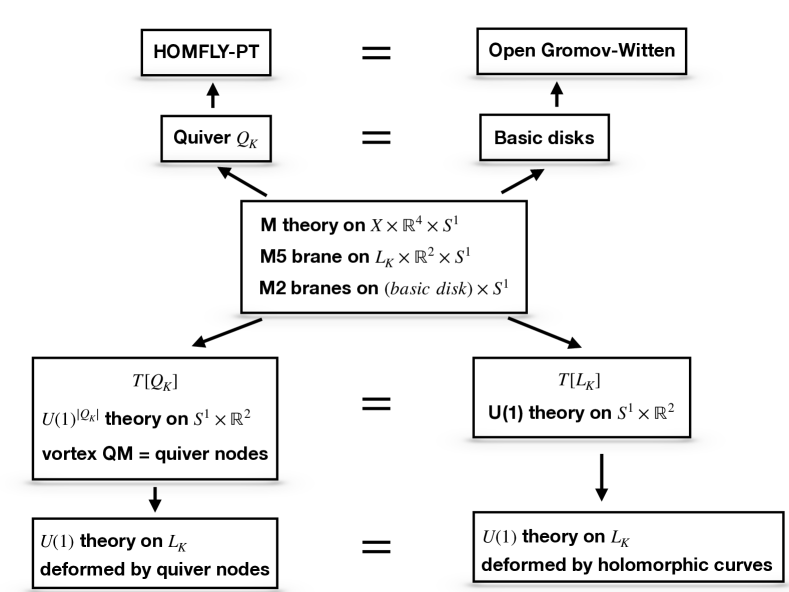
Figure 1: Physics and geometry of knots and quivers – schematic overview

1.1 Physical picture

As shown in Figure 1, the starting point of our physical and geometric considerations is the large $N$ description of colored HOMFLY-PT polynomials as Gromov-Witten invariants of the knot conormal $L_{K}$ in the resolved conifold $X$, see Ooguri:1999bv ; Aganagic:2013jpa ; ES . From the M-theory point of view, the generating series of HOMFLY-PT polynomials counts M2-branes wrapping holomorphic curves with boundary on an M5-brane wrapping the knot conormal. The complete M-theory background is $X\times S^{1}\times\mathbb{R}^{4}$, where the M5-brane wraps $L_{K}\times S^{1}\times\mathbb{R}^{2}$ and the M2-branes wrap the product of a holomorphic curve and $S^{1}$.

There are two effective descriptions of the low energy dynamics on the M5-brane, see Figure 1. First, in terms of a $U(1)$ Chern-Simons gauge theory on $L_{K}$, which from the geometric point of view is ordinary $U(1)$ Chern-Simons theory deformed by certain embedded holomorphic disks, introducing curvature concentration along their boundaries. Second, in terms of a 3d ${\mathcal{N}}=2$ theory $T[L_{K}]$ on $S^{1}\times{\mathbb{R}}^{2}$ Dimofte:2010tz ; Terashima:2011qi ; Dimofte:2011ju ; Yag1305 ; LY1305 ; Cordova:2013cea .

We introduce a novel dual description of $T[L_{K}]$, as an Abelian Chern-Simons-matter theory $T[Q_{K}]$, which features a $U(1)$ gauge group and a single fundamental chiral for each node of $Q_{K}$. Interactions between the sectors corresponding to single nodes are governed by Chern-Simons couplings (encoded in the quiver arrows) and Fayet-Ilioupoulos (FI) couplings. Recall that the FI couplings may also be viewed as mixed Chern-Simons terms between the gauge $U(1)$ factors and their dual topological symmetries. Global symmetries of $T[Q_{K}]$ include rotations of the base ${\mathbb{C}}{\mathbb{P}}^{1}$ of $X$, as well as rotations of ${\mathbb{R}}^{2}\times{\mathbb{R}}^{2}\simeq{\mathbb{R}}^{4}$ twisted by a $U(1)_{R}$ action on $X$. Fugacities of these symmetries are often denoted by $(a,q,t)$ in the context of knot polynomials Fuji:2012nx ; DGR0505 . In this context, the FI couplings give the change of variables $x_{i}\sim a^{a_{i}}q^{q_{i}-t_{i}}t^{t_{i}}$, where $x_{i}$ is the variable associated to the $i^{\rm th}$ quiver node in $T[Q_{K}]$, that identifies the Poincaré generating series of quiver representation varieties of the series of symmetric-colored superpolynomials. Here the HOMFLY-PT polynomial is recovered by specializing to $t=-1$. In other words, FI couplings encode the relation between global and topological symmetries of $T[Q_{K}]$.

The dual description $T[Q_{K}]$ encoded by the quiver has several advantages over descriptions of type $T[L_{K}]$, previously adopted in the literature. One of these is the fact that the structure of $T[Q_{K}]$ is fully and explicitly known, while $T[L_{K}]$ can be rather complicated and not fully understood even for simple knots. Another important feature of $T[Q_{K}]$ is the fact that it bridges between counts of holomorphic curves (via duality with $T[L_{K}]$) and quiver descriptions of corresponding BPS states, hence providing a key link in the knots-quivers correspondence. The M2-branes with boundary on the M5-brane give rise to BPS vortices of $T[Q_{K}]$. It was recently observed that the BPS vortex spectrum of certain 3d ${\mathcal{N}}=2$ theories admits a quiver quantum mechanics description Hwang:2017kmk . Here we think of the vortex quantum mechanics of $T[Q_{K}]$ as the physical origin of the quiver $Q_{K}$. The existence of a quiver description of vortices then leads to the quiver description of knot invariants observed in Kucharski:2017poe ; Kucharski:2017ogk . The quiver of vortices and $Q_{K}$ arise as effective descriptions of the underlying M-theory system, which consists of M2-branes ending on an M5-brane. The BPS vortex spectrum of the theory $T[Q_{K}]$ is the shadow (effective description) of this theory on the  $\mathbb{R}^{2}\times S^{1}$ part of the M5-brane, and is governed by the ${\mathcal{N}}=2$ quantum mechanics of vortices. The quiver $Q_{K}$, on the other hand, is the shadow of the theory on $X$ and describes the  ${\mathcal{N}}=4$ quantum mechanical dynamics of M2-branes that are standardized (stretched in sympletic language) near $L_{K}$.

Quiver descriptions of BPS spectra are known to arise in string theory as a way to encode all BPS states as boundstates of a finite set of basic BPS generators. Such descriptions are well understood in the context of 4d ${\mathcal{N}}=2$ quantum field theories, where BPS generators are identified with nodes of the quiver, and intersections between corresponding M2-branes are encoded by arrows connecting the nodes Denef:2002ru ; Alim:2011kw ; Gabella:2017hpz . We will see that the this framework is line with interpretations of $Q_{K}$ given in this paper.

1.2 Geometric picture

Another core result of the present work is the introduction of a geometric point of view behind the quiver description of holomorphic curves (and by extension, knot invariants). We first describe the geometric objects involved and then formulate a precise conjecture. The quiver nodes or BPS generators correspond to basic embedded holomorphic disks with boundary on $L_{K}$ and with a framing along the boundary. The Gromov-Witten potential counts generalized holomorphic cvurves Ekholm:2018iso ; iacovino1 ; iacovino2 ; iacovino3 with boundary on $L_{K}$. From the point of view of ES , generalized holomorphic curves are bare curves with boundary in the $U(1)$ skein module projected to homology class and linking (encoded in the $q$-power).

For the quiver description, the holomorphic curve components of all generalized holomorphic curves lie in a small neighborhood of the union of $L_{K}$ with the basic disks attached. This space can be thought of as a deformation of $T^{\ast}L_{K}$, which describes a symplectic neighborhood of $L_{K}$ when there are no non-constant holomorphic disks ending on it. Here each sector of $T[Q_{K}]$, consisting of a $U(1)$ gauge theory and its fundamental chiral, corresponds to ordinary $U(1)$ Chern-Simons theory deformed by all generalized holomorphic curves that contain at least one copy of a fixed basic holomorphic disk.

The FI couplings for the $i^{\rm th}$ basic holomorphic disk correspond (roughly) to its homology class in $H_{2}(X)$ ($a_{i}$) and to the Euler characteristics of the curves in a neighborhood of the disk, $e^{q_{i}\frac{1}{2}g_{s}}$ related to intersections with a 4-chain $C_{K}$ with boundary $2\cdot L_{K}$ ($q_{i}$ and $t_{i}$). The Chern-Simons couplings encoded in quiver arrows here correspond to linking and self-linking numbers of boundaries of basic holomorphic disks as embedded curves in $L_{K}$, where linking numbers are defined only up to a choice of longitude on the boundary torus. Then the quiver expression for the partition function corresponds to the count of all generalized holomorphic curves constructed from linked configurations of the basic disks. The 4-chain $C_{K}$ mentioned above is a familiar object in the context of knot contact homology Ekholm:2018iso . From the physical point of view, it is reminiscent of a family of Dirac strings and we discuss an interpretation in that spirit from the M-theory perspective in Section 6.3.

The above discussion can be summarized and made precise in a conjecture that we state next. Let $\psi_{K}(x,a,e^{\frac{1}{2}g_{s}})$ denote the Gromov-Witten partition function counting all (disconnected) generalized holomorphic curves ending on $L_{K}$. This has the well-known structure of a generating series

$$\psi_{K}(x,a,e^{\frac{1}{2}g_{s}})=\sum_{r\geq 0}P^{K}_{r}(a,q)x^{r},$$ (1)

where $P^{K}_{r}(a,q)$ is the HOMFLY-PT polynomial of $K$ in the $r^{\rm th}$ symmetric representation Ooguri:1999bv ; ES ; Ekholm:2018iso . We may also consider a refinement of this partition function, denoted $\Psi_{K}(x,a,q,t)$, where the coefficient of $x^{n}$ is the superpolynomial $\mathcal{P}^{K}_{r}(a,q,t)$ (Poincaré polynomial of the HOMFLY-PT homology DGR0505 ), so that $\psi_{K}(x,a,q)=\Psi_{K}(x,a,q,t=-1)$.

Conjecture 1.1.

Let $K\subset S^{3}$ be a framed knot and let $L_{K}\subset X$ be its Lagrangian conormal shifted off the zero section and considered a Lagrangian in the resolved conifold. We conjecture that there is a finite number of embedded holomorphic disks $D_{1},\dots,D_{m}$ ending on $L_{K}$ with framed boundaries such that the following holds.

Let $Q_{K}$ be the symmetric quiver with nodes $D_{i}$ and arrows $C_{ij}$ corresponding to linking (and self-linking) numbers $\mathrm{lk}(\partial D_{i},\partial D_{j})$ measured with respect to the framing of $\partial L_{K}$. Let $x_{i}$ be the quiver variable of $D_{i}$, $a_{i}$ denote the homology class of $D_{i}$ in $H_{2}(X)\subset H_{2}(X,L_{K})$, $n_{i}$ the homology class $\partial D_{i}$ in $H_{1}(L_{K})$, and $q_{i}-C_{ii}$ the intersection number $D_{i}\cdot C_{K}$. Then we have

$$\Psi_{K}(x,a,q,t)=P^{Q_{K}}(x_{1},\dots,x_{m},q)|_{x_{i}=x^{n_{i}}a^{a_{i}}q^{q_{i}-C_{ii}}(-t)^{C_{ii}}},$$ (2)

where the right hand side is the quiver partition function, see (45).

We comment on possible proofs of Conjecture 1.1. For $K=0_{1}$, the unknot, the conjecture holds: after representing the unknot conormal as a toric brane there are exactly two holomorphic disks ending on it, see Section 5. For more general knots it is likely that one can find a finite number of disks for the conjecture by degenerating the conormal to the unknot conormal as a braid representative approaches the unknot. Provided the finite collection of disks are found, the Gromov-Witten level of the conjecture could likely be proved combining ES ; Ekholm:2018iso with OP ; KL . We still lack the geometric definition and properties of the refined partition function $\Psi_{K}(x,a,q,t)$, but they are currently being investigated.

The geometric picture in Conjecture 1.1 passes several nontrivial checks, for example its behavior under changes of framing. It also raises new questions, in particular about invariance under deformations of $L_{K}$ and ways of finding all basic disks in general. For simple knots there is one basic disk for each monomial in the HOMFLY-PT polynomial. For more complicated knots that is no longer the case and the quiver description is more involved. We discuss these questions with details in a couple of explicit examples.

1.3 Outline of the paper

The outline of the paper is as follows. Section 2 contains a review of relevant material on knots, quivers, BPS states, and holomorphic disks. In Section 3 we introduce the quiver gauge theory $T[Q_{K}]$ associated to the quiver dual to a knot, and show that its BPS vortex spectrum is captured by the representation theory of $Q_{K}$. In Section 4 we provide a geometric interpretation of quiver representations in terms of generalized holomorphic disks and discuss identification of quiver data with linking and self-linking numbers. Section 5 illustrates our viewpoint on the knots-quivers correspondence on the simplest examples of the unknot and the trefoil. We conclude in Section 6 with a discussion and suggestions for future work.

2 Background

2.1 Knots-quivers (KQ) correspondence

If $K\subset S^{3}$ is a knot, then its HOMFLY-PT polynomial $P^{K}(a,q)$ freyd1985 ; PT is a 2-variable polynomial that is easily calculated from a knot diagram (a projection of $K$ with over/under information at crossings) via the skein relation. The polynomial is a knot invariant, i.e. invariant under isotopies and in particular independent of diagrammatic presentation. More general knot invariants are the colored HOMFLY-PT polynomials $P^{K}_{R}(a,q)$, where $R$ is a representation of the Lie algebra ${\mathfrak{u}}(N)$. Also the colored version admits a diagrammatic description in terms of standard polynomial of certain satellite links of $K$. In this setting, the original HOMFLY-PT corresponds to the standard representation. Below, to simplify notation, we will often write simply the HOMFLY-PT polynomial also when we refer to the more general colored version.

From the physical point of view, the HOMFLY-PT polynomial is the expectation value of the knot viewed as a Wilson line in $U(N)$ Chern-Simons gauge theory witten1989 , which then depends on a choice of representation $R$ for the Lie algebra ${\mathfrak{u}}(N)$. Here we will restrict attention to completely symmetric representations, corresponding to Young diagrams with a single row with $r$ boxes. For each $r$-box representation we get a polynomial $P_{r}^{K}(a,q)$ and we consider the  HOMFLY-PT generating series in the variable $x$

$$P^{K}(x,a,q)=\sum_{r=0}^{\infty}P_{r}^{K}(a,q)x^{r}\,.$$ (3)

In this setting, the Labastida-Mariño-Ooguri-Vafa (LMOV) invariants Ooguri:1999bv ; LM0004 ; LMV0010 are certain numbers assembled into the LMOV generating function $N^{K}(x,a,q)=\sum_{r,i,j}N_{r,i,j}^{K}x^{r}a^{i}q^{j}$ that gives the following expression for the HOMFLY-PT generating series

$$P^{K}(x,a,q)=\mathrm{Exp}\left(\frac{N^{K}(x,a,q)}{1-q^{2}}\right)\,.$$ (4)

Exp is the plethystic exponential – if $f=\sum_{n}a_{n}t^{n}$, $a_{0}=0$, then

$$\mathrm{Exp}\bigl{(}f\bigr{)}(t)=\exp\left(\sum_{k}\tfrac{1}{k}f(t^{k})\right)=\prod_{n}(1-t^{n})^{n\,a_{n}}.$$

According to the LMOV conjecture Ooguri:1999bv ; LM0004 ; LMV0010 $N_{r,i,j}^{K}$ are integer numbers.

The knots-quivers (KQ) correspondence introduced in Kucharski:2017poe ; Kucharski:2017ogk and mentioned in the previous section provides a new approach to HOMFLY-PT polynomials and LMOV invariants. We give a brief discussion.

A quiver $Q$ is an oriented graph with a finite set of vertices $Q_{0}$ connected by finitely many arrows (oriented edges) $Q_{1}$. A dimension vector for $Q$ is a vector in the integral lattice with basis $Q_{0}$, $\mathbf{d}\in{\mathbb{Z}}Q_{0}$. We number the vertices of $Q_{0}$ by $1,2,\dots,m=|Q_{0}|$. A quiver representation with dimension vector $\mathbf{d}=(d_{1},\dots,d_{m})$ is the assignment of a vector space of dimension $d_{i}$ to the node $i\in Q_{0}$ and of a linear map $\gamma_{ij}\colon{\mathbb{C}}^{d_{i}}\to{\mathbb{C}}^{d_{j}}$ to each arrow in $Q_{1}$ from vertex $i$ to vertex $j$. The adjacency matrix of $Q$ is the $m\times m$ integer matrix with entries $C_{ij}$ equal to the number of arrows from $i$ to $j$. A quiver is symmetric if its adjacency matrix is.

Quiver representation theory studies moduli spaces of stable quiver representations (see e.g. kirillov2016quiver for an introduction to this subject). While explicit expressions for invariants describing those spaces are hard to find in general, they are quite well understood in the case of symmetric quivers KS0811 ; KS1006 ; MR1411 ; FR1512 ; 2011arXiv1103.2736E . Important information about the moduli space of representations of a symmetric quiver with trivial potential is encoded in the motivic generating series defined as

$$P^{Q}(\mathbf{x},q)=\sum_{d_{1},\ldots,d_{m}\geq 0}(-q)^{\sum_{1\leq i,j\leq m}C_{ij}d_{i}d_{j}}\prod_{i=1}^{m}\frac{x_{i}^{d_{i}}}{(q^{2};q^{2})_{d_{i}}}\,,$$ (5)

where the denominator is the so-called $q$-Pochhammer symbol

$$(z;q^{2})_{r}=\prod_{s=0}^{r-1}(1-zq^{2s})\,.$$ (6)

Sometimes we will call $P^{Q}(\mathbf{x},q)$ the quiver partition function. We also point out that quiver representation theory involves the choice of an element, the potential, in the path algebra of the quiver, and that the trivial potential is the zero element.

Furthermore, there are so called motivic Donaldson-Thomas (DT) invariants $\Omega_{\mathbf{d},s}^{Q}=\Omega_{(d_{1},...,d_{m}),s}^{Q}$ which can be assembled into the DT generating function

$$\Omega^{Q}(\mathbf{x},q)=\sum_{\mathbf{d},s}\Omega_{\mathbf{d},s}^{Q}\mathbf{x^{d}}q^{s}(-1)^{|\mathbf{d}|+s+1},$$ (7)

where $\mathbf{x^{d}}=\prod_{i}x_{i}^{d_{i}}$. These give the following new expression for the motivic generating series

$$P^{Q}(\mathbf{x},q)=\textrm{Exp}\left(\frac{\Omega^{Q}(\mathbf{x},q)}{1-q^{2}}\right).$$ (8)

The DT invariants have two geometric interpretations, either as the intersection homology Betti numbers of the moduli space of all semi-simple representations of $Q$ of dimension vector $\mathbf{d}$, or as the Chow-Betti numbers of the moduli space of all simple representations of $Q$ of dimension vector $\mathbf{d}$, see MR1411 ; FR1512 . In 2011arXiv1103.2736E there is a proof that these invariants are positive integers.

The most basic version of the conjectured knot-quiver correspondence is the statement that for each knot $K$ there exists a quiver $Q_{K}$ and integers $\{a_{i},q_{i}\}_{i\in{Q_{K}}_{0}}$, such that

$$\left.P^{Q_{K}}(\mathbf{x},q)\right|_{x_{i}=xa^{a_{i}}q^{q_{i}-C_{ii}}}=P^{K}(x,a,q)\,.$$ (9)

We call $x_{i}=xa^{a_{i}}q^{q_{i}-C_{ii}}$ the KQ change of variables. The purpose of the shift by the number of loops and the meaning of $a_{i},q_{i}$ are discussed in Section 2.3.

In Kucharski:2017poe ; Kucharski:2017ogk there are also refined versions of the KQ correspondence, as well as the one on the level of LMOV and DT invariants. We can obtain it by substituting (4) and (8) into (9)

$$\left.\Omega^{Q_{K}}(\mathbf{x},q)\right|_{x_{i}=xa^{a_{i}}q^{q_{i}-C_{ii}}}=N^{K}(x,a,q)\,.$$ (10)

Since DT invariants are integer, this equation implies the LMOV conjecture. In Sections 2.2, 3.1, 3.3 we will see that the physical meaning of (10) is that DT and LMOV invariants count BPS states in dual 3d $\mathcal{N}=2$ theories. We also have a geometrical interpretation of these invariants as counts of what we call semi-basic holomorphic disks that can loosely be described as embedded generalized holomorphic disks.

We stress that the KQ correspondence is conjectural, and that it is currently not known how to construct the quiver $Q_{K}$ from a given knot $K$. Evidence for the conjecture includes checks on infinite families of torus and twist knots. A proof for 2-bridge knots appeared recently in Stosic:2017wno , whereas PSS1802 explores the relation to combinatorics of counting paths. On the other hand, PS18 contains a relation between quivers and topological strings on various Calabi-Yau manifolds. In this paper we study the KQ correspondence from the point of view of large $N$ transition and discuss how to interpret the quiver in terms of gauge theoretic reductions of M-theory and in terms of Calabi-Yau reductions as basic holomorphic disks in the spirit of Ooguri:1999bv ; Gopakumar:1998ii ; Gopakumar:1998jq .

2.2 BPS states

Both sides of the KQ correspondence have physics counterparts schematically shown in diagram (11). First, knots as Wilson loops in Chern-Simons theory are related to open topological strings with branes on the knot cononormal $L_{K}$ and the zero-section $S^{3}$ in the cotangent bundle $T^{\ast}S^{3}$ Witten:1992fb ; ES . Via large $N$ duality, this open string in $T^{\ast}S^{3}$ is further related to the open string in the resolved conifold $X$, where $S^{3}$ disappeared and only branes on $L_{K}$ remained, see Ooguri:1999bv ; ES . Second, quiver representation theory appears in the description of how BPS states in several contexts, e.g. in string theory and supersymmetric QFT Denef:2002ru ; Douglas:1996sw ; Fiol:2000wx ; Alim:2011ae , generate more general states.

$$\begin{array}[]{ccc}\text{knots}&\quad\ext@arrow 3359$\leftarrow \xleaders\hbox{$\relbar$}\hfill\rightarrow${\ \ \text{\footnotesize KQ corr.}}&\text{quiver rep. theory}\\ {\left\updownarrow\vbox to17.07182pt{}\right.\kern-1.2pt}&&{\left\updownarrow\vbox to17.07182pt{}\right.\kern-1.2pt}\\ \text{topological strings}&\quad\ext@arrow 9999{\arrowfill@\leftarrow\relbar\rightarrow}{}{\ \ \text{\footnotesize\phantom{KQ corr.}}}&\text{BPS vortices}\\ \end{array}$$ (11)

In this paper we study the origin of the KQ correspondence from the viewpoint of these related physics pictures. This section gives a brief overview of these subjects, see Section 3 for new results followed by a more detailed discussion.

A more precise characterization of the relation between knots and topological strings is as follows. $U(N)_{\kappa}$ Chern-Simons theory on $S^{3}$ ($\kappa$ denotes the level) is related to topological strings on the resolved conifold $X$ with the following matching of parameters:

$$g_{s}=\frac{2\pi i}{\kappa+N}\,,\qquad\qquad\mathtt{t}=\frac{2\pi iN}{\kappa+N}\,,$$ (12)

where $g_{s}$ denotes the string coupling constant and $\mathtt{t}$ is the Kähler parameter of $X$.

The equality of vacuum partition functions for these theories led to the conjecture that these theories are exactly equivalent in the large $N$ limit Witten:1992fb ; ES ; GV9811 . Inserting a Wilson loop supported on a knot $K\subset S^{3}$ on the Chern-Simons side corresponds to considering an A-brane supported on the Lagrangian conormal $L_{K}\subset T^{\ast}S^{3}$ shifted off the zero-section and then considered as a submanifold of $X$. Here, Wilson loop expectation values correspond to open topological string amplitudes for Riemann surfaces with boundary on $L_{K}$. Let us multiply $X$ by $\mathbb{R}^{4}\times S^{1}$ and consider the open topological string as a reduction of M-theory. The relation to open strings can then be interpreted as a relation between Chern-Simons knot invariants, like the HOMFLY-PT polynomial, and the BPS spectrum of M2-branes (corresponding to the most basic holomorphic curves) ending on M5-branes wrapped on $L_{K}$ Ooguri:1999bv .

From the perspective of mirror symmetry we can construct a B-model mirror of $X$ as a conic bundle over a complex torus $\mathbb{C}^{\ast}_{\xi}\times\mathbb{C}^{\ast}_{\eta}$, corresponding to the two generators $\xi$ and $\eta$ of $H_{1}(\Lambda_{K})$, where $\Lambda_{K}$ is the torus at infinity of $L_{K}$, that degenerates over a curve $V_{K}$. (The standard notation is $(x,p)$ or $(x,y)$, see e.g. Aganagic:2013jpa , but we use $\xi$ and $\eta$ not to confuse with our other uses of $x$.) This curve is known as the mirror curve and can be thought of as the moduli space of $L_{K}$ deformed by disk instanton corrections Aganagic:2000gs . The curve $V_{K}$ comes equipped with a canonical differential $\eta d\xi$. The open topological string wavefunction

$$\Psi_{K}(\xi)=\exp\left(\sum_{n}C_{n}(e^{\mathtt{t}},g_{s})e^{n\xi}\right)$$ (13)

counts (generalized) holomorphic curves in $X$ with boundary on $L_{K}$, see Ekholm:2018iso . Up to conventions and the change of variables

$$e^{\mathtt{t}}=a^{2},\qquad e^{g_{s}}=q^{2},\qquad e^{\xi}=x\,,$$ (14)

the wavefunction $\Psi_{K}(\xi)$ is equal to the HOMFLY-PT generating series $P^{K}(x,a,q)$, see equation (1).

The semiclassical limit $g_{s}\to 0$ of $\Psi_{K}(\xi)$ recovers the Gromov-Witten disk potential $W_{K}(\xi)$ that is computed by the Abel-Jacobi map on the mirror curve Aganagic:2000gs ; Aganagic:2001nx

$$\Psi_{K}(\xi)\sim\exp\left(\frac{1}{g_{s}}\int\eta d\xi+\dots\right)=\exp\left(\frac{1}{g_{s}}W_{K}(\xi)+\dots\right)\,.$$ (15)

As mentioned above, basic holomorphic curves with boundary on $L_{K}$ appear as reductions of M2-branes wrapping the curve ending on M5-branes which wrap $L_{K}$.

We next consider another reduction of M-theory: BPS counting of M2-branes can be formulated in terms of world volume dynamics on the M5-brane wrapped on $L_{K}\times{\mathbb{R}}^{2}\times S^{1}$. The corresponding low energy theory $T[L_{K}]$ is a 3d ${\mathcal{N}}=2$ Chern-Simons matter gauge theory on ${\mathbb{R}}^{2}\times S^{1}$. Its field content and couplings are determined by the geometry of $L_{K}\subset X$ Dimofte:2010tz ; Dimofte:2011ju . These low energy theories have interesting spectra of BPS vortices counted by LMOV invariants. BPS vortices arise from M2-branes that wrap holomorphic curves with boundary on $L_{K}$ and that stretch along the $S^{1}$-direction in $X\times\mathbb{R}^{4}\times S^{1}$. In fact, vortices can be localized at the origin of the worldvolume ${\mathbb{R}}^{2}$ by turning on an $\Omega$-background Shadchin:2006yz .

BPS states are the lightest charged particles in a supersymmetric QFT, characterized by the requirement that their mass is linearly proportional to their charge under gauge and global symmetries Witten:1978mh . In consequence, BPS states are invariant under half of the supersymmetry (two supercharges in our case), leading to additional constraints on their dynamics. (These constraints give rise to interesting phenomena typical of BPS states, like wall-crossing.) BPS dynamics play a fundamental role in the characterization of the 3d ${\mathcal{N}}=2$ BPS vortex spectrum. Generally speaking, global symmetries act on the Hilbert space of BPS states $\mathcal{H}^{\rm BPS}$ which is therefore naturally graded by the corresponding charges (such as spin or magnetic flux): $\mathcal{H}^{{\rm BPS}}=\bigoplus_{\gamma}\mathcal{H}^{{\rm BPS}}_{\gamma}$.

In addition to the natural grading by charges, there is a second and more refined type of grading on $\mathcal{H}^{{\rm BPS}}$, which depends on the details of the theory. While the spectrum of BPS vortices is often infinite, under certain conditions it can be organized into boundstates of a finite set $Q_{0}$ of fundamental BPS states of lowest charge, thus introducing a ${\mathbb{Z}}Q_{0}$ grading on $\mathcal{H}^{{\rm BPS}}$ Hwang:2017kmk . A bound state consisting of $d_{i}$ copies of the $i$-th fundamental vortex is labeled by a dimension vector $\mathbf{d}$, and its properties (e.g. the number and spin of ’internal’ configurations, or its BPS degeneracies) can be modeled by the world line quantum mechanics of the multi-particle system. Let $QM({\mathbf{d}})$ denote this theory.

Supersymmetry imposes constraints on the types of multiplets and interactions in the quantum mechanical description, for more details see Hori:2014tda . In the case of ${\mathcal{N}}=4$ quantum mechanics, the interactions are governed by an integer matrix $C_{ij}$ with $i,j\in Q_{0}$ and a superpotential $W$. This data can be encoded in a quiver, as described in the previous section. In particular, the problem of computing the supersymmetric vacua of $QM({\mathbf{d}})$ reduces precisely to the study of representation theory of $Q$ corresponding to the dimension vector $\mathbf{d}$. This then gives the rightmost arrow in diagram (11), connecting quivers to BPS vortices of 3d ${\mathcal{N}}=2$ theories $T[L_{K}]$. In Section 3 we give explicit descriptions of these theories, and of their BPS vortex spectra.

More precisely, while BPS vortices of $T[L_{K}]$ can be described by a quiver, this is not yet the one appearing in the KQ correspondence. In fact, theories with ${\mathcal{N}}=2$ supersymmetry enjoy a rich duality web, and one of the main messages of this paper is that $T[L_{K}]$ has a dual description $T[Q_{K}]$ whose vortex spectrum is described by the quiver quantum mechanics of the quiver $Q_{K}$ of Kucharski:2017poe ; Kucharski:2017ogk . The full extent of this relation will be explored in Section 3.

Another important point is that the vortex spectrum of a 3d ${\mathcal{N}}=2$ theory is generically described by ${\mathcal{N}}=2$ quantum mechanics. This admits a quiver description too, albeit with more than one type of arrow connecting the nodes Hwang:2017kmk . The quiver $Q_{K}$ on the other hand should be regarded as encoding data of a ${\mathcal{N}}=4$ quantum mechanics. The relation between this and the ${\mathcal{N}}=2$ vortex quantum mechanics may be roughly summarized by saying that the former describes the dynamics of holomorphic disks, and the latter the dynamics of vortices. Such a relation between quivers with different amounts of supersymmetry appears to be novel, it is illustrated and further discussed in Section 3.5 with an explicit example.

To conclude the overview, it is worth noting that a ${\mathcal{N}}=4$ quiver quantum mechanics description of boundstates of M2-branes wrapping holomorphic curves with boundaries on an M5-brane appeared in the context of BPS spectra of 4d ${\mathcal{N}}=2$ theories Alim:2011kw ; Alim:2011ae . In fact this is not unrelated to our setup, we will return to this point in Section 6.

2.3 Knot homologies and A-polynomials

The physics and geometry of the KQ correspondence involves not only HOMLFY-PT polynomials and LMOV invariants, but also other knot-theoretical objects like HOMFLY-PT homology and A-polynomials.

The first well understood knot homologies were introduced in Khovanov ; KhR1 ; KhR2 , however for the KQ correspondence the most relevant is HOMFLY-PT homology which was proposed in DGR0505 as a categorification of the uncolored reduced HOMLFY-PT polynomial

$$P_{1}^{K,\textrm{reduced}}(a,q)=\sum_{i,j}(-1)^{k}a^{i}q^{j}\dim\mathscr{H}_{i,j,k}^{\textrm{reduced}}(K).$$ (16)

Considering the Poincaré polynomial instead of the Euler characteristic provides a $t$-refinement leading to knot invariant called the (uncolored reduced) superpolynomial

$$\mathcal{P}_{1}^{K,\textrm{reduced}}(a,q,t)=\sum_{i,j,k}a^{i}q^{j}t^{k}\dim\mathscr{H}_{i,j,k}^{\textrm{reduced}}(K).$$ (17)

We work with unreduced normalization and consider the finite dimensional unreduced homology $\mathscr{H}(K)$ GNSSS1512 , whose Poincaré polynomial is obtained by multiplying the (reduced) superpolynomial by the unknot numerator, i.e. $1+a^{2}t$. (Our convention for the unknot polynomial, which affects all normalizations of unreduced knot-theoretical objects, will be further detailed in Sections 5.1–5.2.) Therefore

$$\mathcal{P}_{1}^{K}(a,q,t)=\frac{\sum_{i,j,k}a^{i}q^{j}t^{k}\dim\mathscr{H}_{i,j,k}(K)}{1-q^{2}}=\frac{\sum_{i\in\mathscr{G}(K)}a^{a_{i}}q^{q_{i}}t^{t_{i}}}{1-q^{2}},$$ (18)

where we write the sum over $\mathscr{G}(K)$ – the set of generators of $\mathscr{H}(K)$ – to extract powers $a_{i}$, $q_{i}$, and $t_{i}$. The first two turn out to be integers that determine the KQ change of variables mentioned in Section 2.1, whereas $t_{i}$ is equal to $C_{ii}$, the number of loops attached to the $i$-th vertex of the quiver Kucharski:2017poe ; Kucharski:2017ogk . This suggest that the $t$-deformation is encoded in the quiver and indeed can be considered as a refined version of the KQ correspondence

$$\left.P^{Q_{K}}(\mathbf{x},q)\right|_{x_{i}=xa^{a_{i}}q^{q_{i}-C_{ii}}(-t)^{C_{ii}}}=\mathcal{P}^{K}(x,a,q,t)=\sum_{r=0}^{\infty}\mathcal{P}_{r}^{K}(a,q,t)x^{r}\,.$$ (19)

Here $\mathcal{P}^{K}(x,a,q,t)$ is a generating function of $S^{r}$-colored superpolynomials, i.e. Poincaré polynomials of the (finite dimensional unreduced version of) $S^{r}$-colored HOMFLY-PT homology introduced in Gukov:2011ry .

After GGS1304 , we know that HOMFLY-PT homology can be generalized to the quadruply graded homology. Following once again the idea of GNSSS1512 , we can consider the quadruply graded finite dimensional unreduced homology $\tilde{\mathscr{H}}(K)$, but this time the unknot numerator factor reads $1+a^{2}t_{r}t_{c}$. The Poincaré polynomial is given by

$$\tilde{\mathcal{P}}_{1}^{K}(a,Q,t_{r},t_{c})=\frac{\sum_{i,j,k,l}a^{i}Q^{j}t_{r}^{k}t_{c}^{l}\dim\tilde{\mathscr{H}}_{i,j,k,l}(K)}{1-t_{c}^{2}}=\frac{\sum_{i\in\tilde{\mathscr{G}}(K)}a^{a_{i}}Q^{q_{i}}t_{r}^{t_{i}}t_{c}^{t_{i}}}{1-t_{c}^{2}}\,,$$ (20)

where $\tilde{\mathscr{G}}(K)$ is a set of generators of $\tilde{\mathscr{H}}(K)$. We can also consider $\tilde{\mathscr{H}}^{S^{r}}(K)$, a colored generalization of $\tilde{\mathscr{H}}(K)$, and we will call its Poincaré polynomial $\tilde{\mathcal{P}}_{r}^{K}(a,Q,t_{r},t_{c})$. It is a quadruply-graded polynomial which forms a generating series that appears in a doubly refined KQ correspondence Kucharski:2017poe ; Kucharski:2017ogk

$$\left.P^{Q_{K}}(\mathbf{x},q)\right|_{x_{i}=xa^{a_{i}}Q^{q_{i}}(-t_{r})^{C_{ii}},\,q=t_{c}}=\tilde{\mathcal{P}}^{K}(x,a,Q,t_{r},t_{c})=\sum_{r=0}^{\infty}\tilde{\mathcal{P}}_{r}^{K}(a,Q,t_{r},t_{c})x^{r}\,.$$ (21)

Looking at the change of variables we can see the reason of keeping $q_{i}$ and $C_{ii}=t_{i}$ separate in (9).

Equations (18–19) can be obtained from (20–21) by the following substitution

$$Q\mapsto q\,,\qquad t_{r}\mapsto tq^{-1}\,,\qquad t_{c}\mapsto q\,.$$ (22)

Since $t$ comes from $t_{r}$ our refinement is called $t_{r}$. Some authors use an inequivalent $t_{c}$ refinement and unification of both conventions was one of the motivations of introducing four gradings in GGS1304 .

From another viewpoint, A-polynomials are also relevant for the physics and geometry of the KQ correspondence. It was conjectured in AV1204 and proved in GLL1604 that there exists a recursion relation for HOMFLY-PT polynomials which can be encoded in the form

$$\widehat{A}^{K}P_{r}^{K}(a,q)=0,$$ (23)

where the operator $\widehat{A}^{K}$ is the quantum $a$-deformed A-polynomial. See Ekholm:2018iso for a geometric derivation. Further, Fuji:2012nx provided a $t$-refinement with the quantum super-A-polynomial annihilating superpolynomial $\mathcal{P}_{r}^{K}(a,q,t)$. That work predicted that the classical A-polynomial $A^{K}$ arises from the semiclassical limit ($q=e^{\hbar}\rightarrow 1$) of (23) and encodes the supersymmetric vacua of 3d $\mathcal{N}=2$ theory. This phenomenon will be studied in detail in Section 3.1. A-polynomials are also related to geometry of holomorphic disks briefly reviewed in the following section. $A^{K}$ is conjectured AV1204 ; Fuji:2012nx ; Aganagic:2013jpa ; FGSS1209 to agree with augmentation polynomial introduced in Ng0407 ; Ng1010 .

In this paper we will mainly use the dual classical super-A-polynomials $\mathcal{A}^{K}$ GKS1504 which are the $q\rightarrow 1$ limits of operators annihilating the generating function of superpolynomials

$$\widehat{\mathcal{A}}^{K}\mathcal{P}^{K}(x,a,q,t)=0$$ (24)

and therefore are closer to the KQ correspondence. Here $\mathcal{A}^{K}$ and $A^{K}$ are related by a change of variables mentioned in Section 5.1 and explained in GKS1504 . For simplicity we will usually skip “dual classical” and call $\mathcal{A}^{K}$ a super-A-polynomial.

2.4 Holomorphic disks and generalized holomorphic curves

In this section we give a brief description of the material of Section 2.2 from a more geometric point of view. The starting point is to view open Gromov-Witten theory of a Maslov index zero Lagrangian submanifold $L$ in a Calabi-Yau 3-fold $Y$ as the holomorphic curves with boundary on $L$ deforming the Chern-Simons theory in $L$. From a mathematical point of view, this was recently interpreted as Gromov-Witten invariants with values in the skein module of $L$, see ES . Combining this viewpoint in the case $Y=T^{\ast}S^{3}$ with a certain deformation of almost complex structures, known as Symplectic Field Theory stretching, in fact leads to new understanding of the geometric mechanism responsible for large $N$ duality.

As above we consider the Lagrangian conormal $L_{K}$ of a knot $K\subset S^{3}$ shifted off the zero section as a Lagrangian in the resloved conifold $X$. The argument above then shows as conjectured that the HOMFLY-PT polynomials of $K$ are identified with open Gromov-Witten invariants of $L_{K}\subset X$. More precisely, the wave function $\Psi_{K}(\xi)$ of $L_{K}$ can be written as

$$\Psi_{K}(\xi)=\exp\left(\sum_{n\geq 1}C_{n}(e^{\mathtt{t}},g_{s})e^{n\xi}\right),$$ (25)

where $C_{n}(e^{\mathtt{t}},g_{s})$ is a polynomial in $e^{\mathtt{t}}$ that counts (connected) generalized holomorphic curves with boundary in homology class $n\xi\in H_{1}(L_{K})$, where $\mathtt{t}$ corresponds to the homology class in $H_{2}(X)$ after capping $n\xi$ off.

In Aganagic:2013jpa ; Ekholm:2018iso rather effective indirect approaches to calculating $\Psi_{K}(\xi)$ were described. The main idea is to use punctured holomorphic curves at infinity (which are controlled by so called Morse flow trees that can be calculated combinatorially from a braid representation of the knot, see Ekholm:2018iso ) and their interactions with the closed curves that contribute to the wave function. In Aganagic:2013jpa this led to a calculation of the disk potential and the mirror curve by elimination theory in finitely many variables. The calculation also identifies the polynomial of the mirror curve with the augmentation polynomial $\mathrm{Aug}_{K}$ of knot contact homology. In a similar way the full genus counterpart of knot contact homology gives the quantization of $\mathrm{Aug}_{K}$, which is an operator $\widehat{\mathrm{Aug}}_{K}$ annihilating $\Psi_{K}$. The arguments relating curves at infinity to curves in the bulk are of wall crossing type. Briefly, one looks at $1$-parameter family of curves that starts out at infinity, as we push the curve into the bulk its boundary crosses the boundary of the bulk curves and to understand the moduli space we glue the curves. The resulting cobordism then give the equations for the curves in the bulk.

In order to connect this picture to quivers, we need to introduce the concept of generalized holomorphic curve. Here we sketch the basic idea, a more precise characterization will be given in Section 4. Let us consider the conormal Lagrangian in the resolved conifold, $L_{K}\subset X$. As discussed in Aganagic:2013jpa the naive count of holomorphic curves is not invariant under deformations. However, if rather than counting curves, we count all potential curves keeping track of all possible gluings under deformations, then the count is invariant. As described in Ekholm:2018iso , such count requires extra geometric data: a certain Morse function on $L_{K}$ and a 4-chain $C_{K}$ with boundary $\partial C_{K}=2\cdot L_{K}$ compatible with $f$ near its boundary. Here the Morse function is used to construct bounding chains in $L_{K}$ for the boundaries of the holomorphic curves, which together with a choice of a longitude at infinity allows us to define the linking number between two curve boundaries. The 4-chain is closely related and we count intersections between the 4-chain and the interiors of the holomorphic curves. In this context a generalized holomorphic curve is a graph with actual holomorphic curves at its vertices and with oriented edges corresponding to linking intersections and, when connecting to the same vertex, to intersections with $C_{K}$. In the language of ES this corresponds to Gromov-Witten invariants with values in the $U(1)$-skein module of $L_{K}$ projected to the homology class in $H_{1}(L_{K})$ and keeping track of the writhe through the $q$-power.

It is not hard to see that holomorphic disks going once around the generator $\xi$ are generically embedded and can never be further decomposed. Assuming, in line with Gopakumar:1998ii ; Gopakumar:1998jq , that all other holomorphic curves are obtained from combinations of branched covers of these and constant curves at their boundary, the count of curves is exactly the quiver partition function with nodes at the basic disks and with arrows according to linking and additional contributions from the vertices given by $4$-chain intersections.

From this point of view, the theory $T[Q_{K}]$ can be thought of as changing the perspective and treating the basic holomorphic disks as independent objects with the Lagrangian attached. As we shall see below, this in particular leads to a separation of the effects of the various basic disks.

3 KQ correspondence and 3d $\bf{\mathcal{N}=2}$ physics

In this section we derive the relation between a knot $K$ and a 3d ${\mathcal{N}}=2$ theory $T[Q_{K}]$, whose BPS vortex partition function coincides with the quiver partition function of $Q_{K}$.

Our starting point will be M-theory on the resolved conifold, with a single M5-brane wrapping the knot conormal $L_{K}$

$$\begin{split}\text{space-time}:\quad&{\mathbb{R}}^{4}\times S^{1}\times X\\ &\cup\phantom{\ \times S^{1}\times\ \ }\cup\\ \text{M5}:\quad&{\mathbb{R}}^{2}\times S^{1}\times L_{K}\end{split}$$ (26)

The effective theory on ${\mathbb{R}}^{2}\times S^{1}$ is expected to be a 3d ${\mathcal{N}}=2$ theory Terashima:2011qi ; Dimofte:2011ju , which we will denote by $T[L_{K}]$. Roughly speaking, this theory is defined by the requirement that its manifold of supersymmetric vacua coincides with the moduli space of flat $U(1)$ connections on the complement of the boundaries of holomorphic disks on $L_{K}$, compare Cordova:2013cea ; Chung:2014qpa . This class of supersymmetric theories is characterized by a rich duality web, and there are several dual theories with the same moduli space.

3.1 The theories $T[L_{K}]$ and $T_{0}[L_{K}]$

Before studying the theory $T[L_{K}]$ itself, it will be helpful to take an intermediate step and study a closely related theory that we denote $T_{0}[L_{K}]$. Just like $T[L_{K}]$, the definition of $T_{0}[L_{K}]$ is based on the requirement that its moduli space of supersymmetric vacua coincides with the moduli space of flat connections on $L_{K}$ in the complement of holomorphic disks. The basic quantity in the theory $T[L_{K}]$ is the holonomy of the longitude in the torus at infinity whereas for $T_{0}[L_{K}]$ it is that along the meridian.

As a side remark, note that the meridian is the generator of the first homology of the knot complement $S^{3}\setminus K$ and the theory $T_{0}[L_{K}]$ is therefore connected to the study of holomorphic curves with boundary on a Lagrangian with the topology of the knot complement, see Aganagic:2013jpa ; 2012arXiv1210.4803N .

One way to construct a theory such as $T_{0}[L_{K}]$ with a suitable space of vacua was proposed in Fuji:2012nx using the reduced normalization of the superpolynomial. Here we use the unreduced normalization which is closer to counts of holomorphic disks, and therefore more useful for explaining the physical origin of quivers associated to knots.

The twisted superpotential of $T_{0}[L_{K}]$ is encoded by the combined large-color and $\hbar\to 0$ limit of the colored superpolynomial

$$\mathcal{P}^{K}_{r}(a,q,t)\ \mathop{\longrightarrow}^{\hbar\to 0}_{r\to\infty}\ \int\prod_{i}\frac{dz_{i}}{z_{i}}\,\exp{\frac{1}{2\hbar}\left(\widetilde{\mathcal{W}}_{T_{0}[L_{K}]}(z_{i},a,t,y)+O(\hbar)\right)}\,.$$ (27)

Here $q=e^{\hbar}$ and we always work in the regime $|q|<1$, whereas $y$ is the value approached by $q^{2r}$ in the limit. The twisted superpotential $\widetilde{\mathcal{W}}_{T_{0}[L_{K}]}$ is a function of several fugacities:

• is associated to the global symmetry $U(1)_{M}$, whose connection arises from the reduction of the 6d abelian 2-form along the meridian cycle of a $T^{2}$ neihgborhood of $K$, therefore it is also identified with the meridian holonomy of a flat connection on $L_{K}$. While the meridian cycle is contractible in $L_{K}$ alone, a connection deformed by the presence of holomorphic curves on $L_{K}$ can have nontrivial meridian holonomy.

• is the fugacity of the global symmetry $U(1)_{Q}$ arising from the internal 2-cycle in the resolved conifold geometry. After the geometric transition this is identified with the base ${\mathbb{C}}{\mathbb{P}}^{1}$ of the resolved conifold. Before the transition it is the 2-sphere at infinity in the $T^{*}S^{3}$ fiber.

• is a parameter associated with rotations $U(1)_{F}$ of the normal bundle of ${\mathbb{R}}^{2}\subset{\mathbb{R}}^{4}$.

• are identified with fugacities for the abelian gauge group $U(1)\times\ldots\times U(1)$ and therefore they are not unique: different dual descriptions may involve gauge groups of different ranks. The working definition of these fugacities is $z_{i}\sim q^{2k_{i}}$ for some integer $k_{i}$ in the limit $\hbar\to 0,\,r\to\infty$. We will review this below with some examples.

The twisted superpotential typically includes two main types of contributions: dilogarithms and squares of logarithms

$$\begin{split}\mathrm{Li}_{2}\left(a^{n_{Q}}(-t)^{n_{F}}y^{n_{M}}z_{i}^{n_{i}}\right)\qquad&\longleftrightarrow\qquad\text{(chiral field)}\,,\\ \frac{\kappa_{ij}}{2}\log\zeta_{i}\cdot\log\zeta_{j}\qquad&\longleftrightarrow\qquad\text{(Chern-Simons coupling)}\,.\end{split}$$ (28)

Each dilogarithm is interpreted as the one-loop contribution of a chiral superfield with charges $(n_{Q},n_{F},n_{M},n_{i})$ under the various symmetries, while quadratic-logarithmic terms are identified with Chern-Simons couplings among the various $U(1)$ gauge and global symmetries, with $\zeta_{i}$ denoting the respective fugacities 1983NuPhB.222…45D ; Witten:1993yc ; Hanany:1997vm ; Hori:2000kt ; Dimofte:2011jd .

Integrating over the gauge fugacities $z_{i}$ by a saddle-point approximation gives the twisted effective superpotential of the theory

$$\widetilde{\mathcal{W}}^{\mathrm{eff}}_{T_{0}[L_{K}]}(a,t,y)=\widetilde{\mathcal{W}}_{T_{0}[L_{K}]}(z_{i}^{*},a,t,y)\,,\;\;\text{where}\;\;\left.\frac{\partial\widetilde{\mathcal{W}}_{T_{0}[L_{K}]}(z_{i},a,t,y)}{\partial{z_{i}}}\right|_{z_{i}=z_{i}^{*}}=0\,.$$ (29)

In Fuji:2012nx it was argued that the theory $T_{0}[L_{K}]$ defined in this way has a moduli space of vacua that coincides with the graph of the super-A-polynomial

$$\frac{\partial\widetilde{\mathcal{W}}^{\mathrm{eff}}_{T_{0}[L_{K}]}(a,t,y)}{\partial\log y}=\log x^{-1}\qquad\Leftrightarrow\qquad\mathcal{A}^{K}(x,y,a,t)=0\,.$$ (30)

The slightly unconventional powers of $x^{-1}$ and $y$ arise from a careful match with the literature on knot invariants, as will be discussed further below. With these conventions, $\log y$ is interpreted as a scalar field in the twisted chiral multiplet corresponding to the $U(1)_{M}$ field strength of the 3d ${\mathcal{N}}=2$ theory on a circle. The role of $\log x^{-1}$ as well as the origin of the super-A-polynomial are more naturally understood from the viewpoint of the theory $T[L_{K}]$, to which we now return.

To identify the content of $T[L_{K}]$, we propose to consider the generating series of $S^{r}$-colored superpolynomials and take a slight variation of the double-scaling limit (27):

$$\mathcal{P}^{K} (x,a,q,t)=\sum_{r\geq 0}\mathcal{P}^{K}_{r}(a,q,t)x^{r}$$ (31)

$$\mathop{\longrightarrow}^{\hbar\to 0}_{{\footnotesize\begin{array}[]{c}q^{2r}\to y\\ q^{2k_{i}}\to z_{i}\end{array}}}\int\frac{dy}{y}\int\prod_{i}\frac{dz_{i}}{z_{i}}\ \exp\frac{1}{2\hbar}\left(\widetilde{\mathcal{W}}_{T_{0}[L_{K}]}(z_{i},a,t,y)+\log y\,\log x+O(\hbar)\right)\,.$$ (34)

The 3d ${\mathcal{N}}=2$ theory arising from this procedure differs from the one in (27) by the fact that $U(1)_{M}$ is now gauged, and for the presence of a Chern-Simons coupling between its fugacity and a background $U(1)_{L}$ symmetry with fugacity $x$

$$\widetilde{\mathcal{W}}_{T[L_{K}]}(z_{i},a,t,x,y)=\widetilde{\mathcal{W}}_{T_{0}[L_{K}]}(z_{i},a,t,y)+\log y\,\log x\,.$$ (35)

In three dimensions there is a dual $U(1)$ “topological” symmetry for each $U(1)$ gauge symmetry, whose current is sourced by vortices. The Chern-Simons coupling between a gauge symmetry and its dual topological symmetry is also known as a FI coupling. This is the interpretation of the parameter $\log x$, corresponding to the fact that $x$ is the fugacity associated with $U(1)_{L}$.

The manifold of vacua of $T[L_{K}]$ is naturally identified with (30). In fact, taking first the saddle point with respect to $z_{i}$ leads to

$$\begin{split}\mathcal{P}^{K}(x,a,q,t)&\sim\int\frac{dy}{y}\ \exp\frac{1}{2\hbar}\left(\widetilde{\mathcal{W}}^{\mathrm{eff}}_{T[L_{K}]}(a,t,x,y)+O(\hbar)\right)\,,\end{split}$$ (36)

where

$$\widetilde{\mathcal{W}}^{\mathrm{eff}}_{T[L_{K}]}(a,t,x,y)=\widetilde{\mathcal{W}}^{\mathrm{eff}}_{T_{0}[L_{K}]}(a,t,y)+\log y\,\log x.$$ (37)

Now integrating over $d\log y$ naturally enforces the saddle point equation for this fugacity, which is equivalent to (30)

$$\frac{\partial\widetilde{\mathcal{W}}^{\mathrm{eff}}_{T[L_{K}]}(a,t,x,y)}{\partial\log y}=0\qquad\Leftrightarrow\qquad\mathcal{A}^{K}(x,y,a,t)=0\,.$$ (38)

3.2 Legendre transform

With the above discussion we arrived at the definition of a theory $T[L_{K}]$ described by a twisted superpotential $\widetilde{\mathcal{W}}_{T[L_{K}]}$ whose critical points coincide with those of the Gromov-Witten disk potential $W_{K}$. This has an intuitive physical origin, which is best understood from the viewpoint of the general setup (26). The disk potential counts holomorphic disks ending on $L_{K}$, which in the physical setup are wrapped by M2-branes ending on M5. From the viewpoint of worldvolume of the fivebrane, they give rise to BPS states in the theory $T[L_{K}]$, namely BPS vortices counted by LMOV invariants. These vortices couple to the $U(1)_{M}$ gauge field in the 3d ${\mathcal{N}}=2$ theory, whose fugacity we denoted by $y$. Since the theory is placed on a circle, the worldline of these BPS particles is finite, and the same goes for their contribution to the effective action, which is proportional to $e^{-2\pi R\,E}$. ($E$ is the mass, which equals the absolute value of the ${\mathcal{N}}=2$ central charge for BPS states). Therefore the holomorphic disks deform the theory, introducing contributions to the effective action (this mechanism is familiar, for example, from the context of instanton/particles in 4d/5d Lawrence:1997jr , and for 3d/4d Gaiotto:2008cd ).

As discussed in Sections 2.2 and 2.4, all contributions from holomorphic disks are summed in the disk potential $W_{K}$, which is the effective action. From the viewpoint of $T[L_{K}]$, the disks are sources for the gauge field, therefore the effective action describing their interactions is naturally computed by a Legendre transform. The term $\log y\cdot\log x$ in (35) provides the source-current interaction, and integrating out $y$ leaves the effective theory of the sources, which describes interactions among holomorphic disks.

To make the above statement concrete, let us start by recalling that the open topological string wavefunction $\Psi_{K}$ is equal to the HOMFLY-PT generating series and the disk potential arises in the $\hbar\to 0$ limit

$$\begin{split}P^{K}(x,a,q)\mathop{\sim}^{\hbar\to 0}\exp\left(\frac{1}{2\hbar}W_{K}(a,x)+\dots\right)\,.\end{split}$$ (39)

For simplicity we will work with $t=-1$ in this section, although each statement admits a generalization to the refined case.

On the other hand, taking the semiclassical limit of the same function as defined in (31), and performing the saddle point analysis with respect to $z_{i}$ leads to (36). Then performing the integral in $y$ is equivalent to taking the saddle points $y^{*}(x)$ defined by (38), leading to the promised Legendre transform

$$W_{K}(a,x)=\left(\widetilde{\mathcal{W}}_{T_{0}[L_{K}]}^{\mathrm{eff}}(a,y)+\log y\,\log x\right)\big{|}_{y=y^{*}(x)}\,.$$ (40)

Here $\widetilde{\mathcal{W}}_{T_{0}[L_{K}]}^{\mathrm{eff}}(a,y)$ arises as a twisted superpotential of a weak coupling limit of $T[L_{K}]$ in which we have no source-current interactions.

The statement that $W_{K}$ is a Legendre transform of $\widetilde{\mathcal{W}}^{\mathrm{eff}}_{T_{0}[L_{K}]}$ admits a natural generalization to a much stronger one, which is that the full quantum effective action of the gauge theory coincides with the Fourier transform of the topological string wavefunction $\Psi_{K}$. We will come back to this with a more precise formulation in Section 3.4.

The relation (40) is also natural from the geometric viewpoint. Since $\Psi_{K}$ counts holomorphic curves ending on $L_{K}$, see Section 4, it is clear that $x$ is the holonomy of a $U(1)$ bundle on the M5-brane wrapping $L_{K}$ around the generator of $H_{1}(L_{K})$. From the construction of conormal Lagrangians it is clear that this corresponds to the longitudinal cycle around $K$ Ooguri:1999bv . This explains the appearance of the Legendre transform, since both connections of $U(1)_{L}$ and $U(1)_{M}$ arise respectively as reductions of the 2-form $C_{2}$ on the longitudinal and meridian cycles $(\ell,m)$

$$\begin{split}\log x^{-1}&=\oint_{S^{1}}A_{L}=\int_{S^{1}\times\ell}C_{2}=\oint_{\ell}A\\ \log y&=\oint_{S^{1}}A_{M}=\int_{S^{1}\times m}C_{2}=\oint_{m}A\,.\end{split}$$ (41)

Here $A$ is the reduction of $C_{2}$ along $S^{1}$. Therefore $\log x^{-1}$ and $\log y$ are conjugate with respect to the Weil-Petersson symplectic form on ${\mathcal{M}}_{{\rm flat}}(T^{2})$ (the moduli space of flat connections on the Legendrian torus at infinity).

The Legendre transform relating $W_{K}$ and $\widetilde{\mathcal{W}}^{\mathrm{eff}}_{T_{0}[L_{K}]}$ involves the information of the vacuum manifold given by (30) in the limit $t\to-1$. In turn both of them can be recovered from the A-polynomial or (equivalently) the augmentation polynomial Aganagic:2013jpa :

• Solving $\mathcal{A}^{K}(x,y,a)=0$ for $y$ gives a function that factorizes into a product determined by classical LMOV invariants $b_{r,i}^{K}=\sum_{j}N_{r,i,j}^{K}$ GKS1504

  $$y^{*}(a,x)=\prod_{r\geq 0,i\in{\mathbb{Z}}}(1-a^{i}x^{r})^{r\,b^{K}_{r,i}}=\left(\lim_{\hbar\to 0}\frac{P^{K}(q^{2}x,a,q)}{P^{K}(x,a,q)}\right)\,.$$ (42)

  Integrating this function yields precisely the Gromov-Witten disk potential

  $$W_{K}(a,x)=\int d\log x\ \log y^{*}\,.$$ (43)

• Solving instead for $x^{-1}$ gives a function $(x^{-1})^{*}(a,y)$ which does not necessarily factorize into a form analogous to (42). Integrating this function gives the twisted effective superpotential of the weak coupling limit of $T[L_{K}]$

  $$\widetilde{\mathcal{W}}^{\mathrm{eff}}_{T_{0}[L_{K}]}(a,y)=\int d\log y\ \log(x^{-1})^{*}\,.$$ (44)

We shall note that the convention on our definition of $x,y$ is fixed by the relation to the (semiclassical limit of) the HOMFLY-PT generating series $P^{K}(x,a,q)$. In particular comparing to Fuji:2012nx one can simply perform the following substitutions $x\to y^{1/2},\ y\to x^{-1}$ into the formulae of the reference.

3.3 The theory $T[Q_{K}]$

The knot-quiver correspondence revolves around the observation relating the generating series of knot polynomials and the partition function of representation theory of a certain quiver. As reviewed in Section 2, we can write it as

$$\mathcal{P}^{K}(x,a,q,t)=\left.P^{Q_{K}}(\mathbf{x},q)\right|_{x_{i}=xa^{a_{i}}q^{q_{i}-C_{ii}}(-t)^{C_{ii}}}\,,$$ (45)

where each side can be expanded in the following form

$$\begin{split}&\sum_{r\geq 0}\mathcal{P}^{K}_{r}(a,q,t)x^{r}\\ &\qquad=\left.\sum_{d_{1},\ldots,d_{m}\geq 0}q^{\sum_{1\leq i,j\leq m}C_{ij}d_{i}d_{j}}\prod_{i=1}^{m}\frac{\left((-1)^{C_{ii}}x_{i}\right)^{d_{i}}}{(q^{2};q^{2})_{d_{i}}}\right|_{x_{i}=xa^{a_{i}}q^{q_{i}-C_{ii}}(-t)^{C_{ii}}}\,.\end{split}$$

On the one hand, this is simply a way of rewriting the sum over symmetric representations into a sum over quiver representations labeled by $\bf d$. On the other hand applying (31) directly to $P^{Q_{K}}$ we obtain a new 3d ${\mathcal{N}}=2$ theory $T[Q_{K}]$

$$P^{Q_{K}}(\mathbf{x},q)\mathop{\longrightarrow}^{\hbar\to 0}_{q^{2d_{i}}\to y_{i}}\int\prod_{i\in{Q_{K}}_{0}}\frac{dy_{i}}{y_{i}}\,\exp\frac{1}{2\hbar}\left(\widetilde{\mathcal{W}}_{T[Q_{K}]}(\mathbf{x},\mathbf{y})+O(\hbar)\right)$$ (46)

$$\widetilde{\mathcal{W}}_{T[Q_{K}]}(\mathbf{x},\mathbf{y})=\sum_{i}\mathrm{Li}_{2}(y_{i})+\log\left((-1)^{C_{ii}}x_{i}\right)\,\log y_{i}+\sum_{i,j}\frac{C_{ij}}{2}\log y_{i}\,\log y_{j}\,.$$

The application of the dictionary (28) gives the following structure for $T[Q_{K}]$:

• Gauge group: $U(1)^{(1)}\times\dots\times U(1)^{(m)}$

• Matter content: chiral fields $\Phi_{i}$ with charge $\delta_{ij}$ under $U(1)^{(j)}$

• Gauge Chern-Simons couplings: $\kappa^{\mathrm{eff}}_{ij}=C_{ij}$

• Fayet-Ilioupoulos couplings: $\log\left((-1)^{C_{ii}}x_{i}\right)$

We could redefine $x_{i}$ to absorb the minus sign $(-1)^{C_{ii}}$, however the resulting changes in formulas for DT invariants and A-polynomials are rather disinclining. From the mathematical point of view, the sign is related to the choice of spin structure on $L_{K}$ that enters in the orientation of the moduli spaces of holomorphic curves.

It is straightforward to read off the theory $T[Q_{K}]$ from the quiver: the gauge group is a product of $U(1)$ factors associated to quiver nodes, the matter content consists of a set of chiral multiplets charged under each $U(1)$, and the Chern-Simons couplings coincide with the adjacency matrix of $Q_{K}$. More precisely, $\kappa_{ij}^{\mathrm{eff}}$ denotes the matrix of effective Chern-Simons couplings, they are related to the bare Chern-Simons couplings by a diagonal shift by $1/2$ due to the presence of charged matter Aharony:1997bx .

The change of variables $x_{i}=xa^{a_{i}}q^{q_{i}-t_{i}}(-t)^{t_{i}}$ required by the KQ correspondence amounts to identifying the FI couplings of $T[Q_{K}]$ with specific combinations of the physical fugacities. Recall that Fayet-Ilioupoulos terms can be interpreted as mixed Chern-Simons couplings between each $U(1)^{(i)}$ gauge group and its dual “topological” global symmetry $U(1)^{(i)}_{J}$ Aharony:1997bx . The KQ change of variables signals that the dual symmetry is partially broken to a subgroup $U(1)_{L}\times U(1)_{Q}\times U(1)_{F}$, because the fugacities $x_{i}$ are not all independent. It would be interesting to identify the mechanism responsible for this breaking, in particular from a geometric perspective. In this paper we regard it as part of the data going into the definition of $T[Q_{K}]$.

The Fayet-Ilioupoulos terms therefore turn into the respective mixed Chern-Simons terms

$$\left.\widetilde{\mathcal{W}}_{T[Q_{K}]}\right|_{x_{i}=xa^{a_{i}}q^{q_{i}-t_{i}}(-t)^{t_{i}}} =\sum_{i,j}\frac{C_{ij}}{2}\log y_{i}\,\log y_{j}+\sum_{i}\mathrm{Li}_{2}(y_{i})$$ (47)

$$+\sum_{i}\log x\log y_{i}+a_{i}\log a~{}\log y_{i}+t_{i}\log t\log y_{i}\,.$$

With this identification $T[Q_{K}]$ has the same moduli space of supersymmetric vacua as $T[L_{K}]$, by construction. Among the many dual descriptions of $T[L_{K}]$, the existence of a quiver $Q_{K}$ provides a specific choice. Note that in taking the semiclassical limit we left out the parameters $q_{i}$, because they would contribute to subleading terms. Nevertheless, since they appear in the definition of variables $x_{i}$ on the same footing as $a_{i},t_{i}$, they should also admit an interpretation as couplings to a background symmetry. This is the group of rotations in the plane ${\mathbb{R}}^{2}$ wrapped by the M5-brane, twisted by R-symmetry (see Section 3.4 for a precise definition). We will also provide a geometric interpretation for the origin of this symmetry in Section 4.

While the KQ change of variables is key to making contact with knot invariants, it is interesting to forget for a moment about the relations among various $x_{i}$ and contemplate the message of the existence of a description like $T[Q_{K}]$. The objects charged under the topological symmetry of this theory are its BPS vortices, which in our setup are engineered by M2-branes wrapping holomorphic disks. Adopting the viewpoint outlined in Section 3.2, $x_{i}$ can be regarded as fugacities for different types of sources in the theory, with each source coupling to only one of the gauge fields ($x_{i}$ couples only to $y_{i}$). The topological string wavefunction given by $\mathcal{P}^{K}(x,a,q,t)$ is now replaced by the more refined generating series $P^{Q_{K}}(\mathbf{x},q)$. The semiclassical limit of this gives then a generalization of the Gromov-Witten disk potential, which we call the quiver disk potential

$$W_{Q_{K}}(\mathbf{x})=\lim_{\hbar\to 0}\ 2\hbar\cdot\log\left(P^{Q_{K}}(\mathbf{x},q)\right).$$ (48)

It is identified with the effective action of the theory $T[Q_{K}]$ after Legendre transform

$$W_{Q_{K}}(\mathbf{x})=\widetilde{\mathcal{W}}_{T[Q_{K}]}(\mathbf{x},\mathbf{y})\big{|}_{\mathbf{y}=\mathbf{y}^{*}(\mathbf{x})}\,.$$ (49)

The saddle point $\mathbf{y}^{*}(\mathbf{x})$ is given by

$$\frac{\partial\widetilde{\mathcal{W}}_{T[Q_{K}]}(\mathbf{x},\mathbf{y})}{\partial\log y_{i}}=0\quad\Leftrightarrow\quad A_{i}^{Q_{K}}(\mathbf{x},\mathbf{y})=0\quad\Leftrightarrow\qquad\frac{\partial W_{Q_{K}}(\mathbf{x})}{\partial\log x_{i}}=\log y_{i}\,.$$ (50)

which defines quiver A-polynomials $\mathcal{\mathbf{A}}^{Q_{K}}(\mathbf{x},\mathbf{y})$ in analogy to (38) and (43). Similar objects were introduced in PSS1802 ; PS18 ; Smo2017 , however without references to physical and geometric intepretations discussed here.

Combining (46) with (50) we can find a quiver A-polynomial for arbitrary $Q_{K}$:

$$A_{i}^{Q_{K}}(\textbf{x},\textbf{y})=1-y_{i}-x_{i}(-y_{i})^{C_{ii}}\prod_{j\neq i}y_{j}^{C_{ij}}\,.$$ (51)

The quiver disk potential describes the interactions of a set of basic sources (one for each quiver node) labeled by $x_{i}$, providing the full count of their spectrum of boundstates. This viewpoint leads naturally to a quiver description of the BPS vortex spectrum, we will return to this below. It is important to note that $W_{Q_{K}}(\mathbf{x})$ admits a compact expression in terms of the Donaldson-Thomas invariants of the quiver. In fact since

$$P^{Q_{K}}(\mathbf{x},q)=\textrm{Exp}\left(\frac{\Omega^{Q_{K}}(\mathbf{x},q)}{1-q^{2}}\right)=\prod_{\mathbf{d},s}(q^{s}\mathbf{x^{\mathbf{d}}};q^{2})_{\infty}^{(-1)^{|\mathbf{d}|+s}\Omega_{\mathbf{d},s}^{Q_{K}}}\,,$$ (52)

where

$$(z;q^{2})_{\infty}=\prod_{s=0}^{\infty}(1-zq^{2s})\underset{\hbar\rightarrow 0}{\sim}\exp\left(\frac{1}{2\hbar}\textrm{Li}_{2}(z)+\ldots\right)\,,$$ (53)

it follows that

$$W_{Q_{K}}(\mathbf{x})=\sum_{\mathbf{d},s}(-1)^{|\mathbf{d}|+s}\Omega_{\mathbf{d},s}^{Q_{K}}\textrm{Li}_{2}(\mathbf{x^{\mathbf{d}}})=\sum_{\mathbf{d}}(-\Omega_{\mathbf{d}}^{Q_{K}})\textrm{Li}_{2}(\mathbf{x^{\mathbf{d}}})\,.$$ (54)

Here $\Omega_{\mathbf{d}}^{Q_{K}}$ are numerical Donaldson-Thomas invariants. Each dilogarithm in the quiver disk potential corresponds to a boundstate of basic holomorphic disks encoded by the dimension vector $\mathbf{d}$, the multiplicity of each boundstate is the DT invariant. Our definition

$$\Omega_{\mathbf{d}}^{Q_{K}}=\sum_{s}(-1)^{|\mathbf{d}|+s+1}\Omega_{\mathbf{d},s}^{Q_{K}}$$ (55)

differs slightly from Kucharski:2017poe ; Kucharski:2017ogk because we have $1-q^{2}$ instead of $q^{-1}-q$ in the denominator inside $\textrm{Exp}\left(\frac{\Omega^{Q_{K}}(\mathbf{x},q)}{1-q^{2}}\right)$.

From our perspective, exemplified by the diagram (11), it is clear that these invariants actually count embedded holomorphic disks. Indeed the (semiclassical limit of the) KQ change of variables translates the quiver disk potential to the Gromov-Witten disk potential

$$\left.W_{Q_{K}}(\mathbf{x})\right|_{x_{i}=xa^{a_{i}}}=W_{K}(a,x)\,.$$ (56)

This can be derived by rewriting the HOMFLY-PT generating series as

$$P^{K}(x,a,q)=\textrm{Exp}\left(\frac{N^{K}(x,a,q)}{1-q^{2}}\right)=\prod_{r,i,j}(x^{r}a^{i}q^{j};q^{2})_{\infty}^{-N_{r,i,j}^{K}}\,,$$ (57)

and applying (39) to extract an expression for the disk potential

$$W_{K}(a,x)=\sum_{r,i,j}\left(-N_{r,i,j}^{K}\right)\textrm{Li}_{2}\left(x^{r}a^{i}\right)=\sum_{r,i}\left(-b_{r,i}^{K}\right)\textrm{Li}_{2}\left(x^{r}a^{i}\right)\,.$$ (58)

This is the usual count of holomorphic disks, from its derivation it is clear that it arises from (54) by the KQ change of variables (45).

Equation (56) implies also that we can obtain the A-polynomial of $K$ from the quiver A-polynomial of $Q_{K}$. Since

$$\begin{split}\log y^{*}(x)&=\frac{\partial\left.W_{Q_{K}}(\textbf{x})\right|_{x_{i}=a^{a_{i}}x}}{\partial\log x}\\ &=\sum_{i}\left.\frac{\partial W_{Q_{K}}(\textbf{x})}{\partial\log x_{i}}\right|_{x_{i}=a^{a_{i}}x}=\sum_{i}\left.\log y^{*}_{i}(\textbf{x})\right|_{x_{i}=a^{a_{i}}x}\,,\end{split}$$ (59)

we have

$$y^{*}(x)=\prod_{i}\left.y^{*}_{i}(\textbf{x})\right|_{x_{i}=a^{a_{i}}x}\,,$$ (60)

where $y^{*}(x)$ solves $\mathcal{A}^{K}(x,y)=0$ and $y^{*}_{i}(\textbf{x})$ solves $A_{i}^{Q_{K}}(\textbf{x},\textbf{y})=0$. Note that this has a natural geometric interpretation: $y_{i}^{*}(x)$ are meridian holonomies for the $U(1)$ connection on $L_{K}$ on tubular neighborhoods of the boundaries of basic disks (which also contain boundaries of all their boundstates), their composition adds up to the meridian holonomy on the torus at infinity $y^{*}(x)$.

From the viewpoint of holomorphic disks, the main message of the quiver description of BPS vortices is that all holomorphic disks can be viewed as “boundstates” of a finite set of fundamental basic disks associated with quiver nodes. An analogous phenomenon is well-known to arise in the context of BPS states of 4d ${\mathcal{N}}=2$ theories, where the BPS spectrum of M2-branes ending on a fivebrane often admits a quiver description in terms of a finite set of “basic” disks – we will return to this in Section 6.

Finally, let us briefly comment on the geometric interpretation of the quiver variables $x_{i}$. The refined KQ change of variables (19) is defined by integers $a_{i},q_{i},t_{i}$ which carry a natural geometric meaning. These variables encode topological data of basic holomorphic disks represented by nodes of $Q_{K}$. Classically, the disks are classified by relative homology classes in $X$ with boundary on $L_{K}$: the classical topological data therefore includes the homology class of the disk boundary $\partial\Sigma\in H_{1}(L_{K})$ and the number of wrappings around two-cycles in $H_{2}(X)$. Since $L_{K}$ has topology $S^{1}\times{\mathbb{R}}^{2}$, there is only one cycle that the disc boundary can wrap and all basic disks wrap that cycle exactly once, explaining why $x$ appears with a unit power in (19). Among the two-cycles in $X$, there is of course the resolved conifold base ${\mathbb{C}}{\mathbb{P}}^{1}$: $a_{i}$ counts the number of wrappings of the $i$-th basic disk around this ${\mathbb{C}}{\mathbb{P}}^{1}$. Since we talk about relative homology, it is understood that the wrappings are defined relative to a universal (but non-canonical) choice of capping for the disks. In other words, we choose a reference disk with boundary on the opposite generator of $H_{1}(L_{K})$, and consider its composition with each of the basic disks to form a closed 2-cycle. Then $a_{i}$ is the closed homology class of this closed cycle. Changing the choice capping disk shifts all $a_{i}$ simultaneously by the same amount, which can be absorbed by an overall normalization, leaving $a_{i}-a_{j}$ as the invariant data.

There is in fact another nontrivial two-cycle in the geometry, which is sometimes overlooked: it is the two-sphere linking $L_{K}$. Since $L_{K}$ supports an M5-brane, it sources magnetic flux for the four-form fieldstrength of eleven dimensional supergravity. In the compactification to $X$ with the M5 wrapped on $L_{K}$, this reduces to a two-form on $X$ which has non-vanishing integral on the two-sphere linking $L_{K}$ (we will return to this in Section 4.5). In a situation where the geometry is modified so as to compactify $L_{K}$ and where we place $M\gg 1$ branes on it, the magnetic flux will be proportional to $M$, and indeed the area of this ${\mathbb{C}}{\mathbb{P}}^{1}$ would arise from the usual ’t Hooft limit as $a_{L_{K}}=q^{M}$, or its refined version $a_{L_{K}}=t^{M}(t/q)^{1/2}$ Aganagic:2012hs . However since we keep $M=1$ this contribution to the holomorphic disk action is a quantum effect in our setup, in the sense that it is non-vanishing only for $t,q\neq 1$, and it is visible only at the quantum level.

We therefore propose to identify $t_{i}=C_{ii}$ with the wrappings of the $i$-th basic disk on the two-sphere linking $L_{K}$, whose origin is the M2-M5 coupling via bulk fluxes. Finally, $q_{i}$ counts the self-linking of the $i$-th basic holomorphic disk. Note that it appears in the combination $q_{i}-C_{ii}$ as the power of $q$, which equals the contributions from 4-chain intersections of the disk. An explanation for this will be provided in the next section, in terms of “real” (M2-M2 via M5) and “imaginary” (M2-M5) self-intersections.

3.4 Vortex partition functions as quiver partition functions

In this section we show that the partition function of BPS vortices of $T[Q_{K}]$ coincides exactly with the motivic generating series of the quiver $Q_{K}$. This is the quantum uplift (to finite $\hbar$) of the identification (49) between the quiver disk potential and the  Legendre transform of the twisted effective superpotential of the theory. To put this statement into perspective let us recall again the relation between vortices and knot theory: BPS vortices of the 3d ${\mathcal{N}}=2$ theory $T[L_{K}]$ arise from M2-branes wrapping holomorphic curves ending on $L_{K}$; for this reason the vortex partition function encodes open Gromov-Witten invariants and therefore knot invariants Dimofte:2010tz ; ES .

As a warm-up, let us start with a simple subclass of theories of type $T[Q]$, characterized by a quiver with diagonal adjacency matrix $C_{ij}=\kappa^{\mathrm{eff}}_{i}\delta_{ij}$. The nodes of $Q$ are mutually disconnected, the only arrows are $\kappa^{\mathrm{eff}}_{i}$ loops on the $i$-th node. In this case $T[Q]$ is made of $m=|Q_{0}|$ copies of a $U(1)_{\kappa_{i}}$ gauge theory, each with a single chiral field with charge $+1$. The bare Chern-Simons level of $U(1)^{(i)}$ is related to $\kappa_{i}^{\mathrm{eff}}$ by a half-integer shift induced by quantum corrections from the charged chiral multiplets Aharony:1997bx :

$$\kappa_{i}=\kappa^{\mathrm{eff}}_{i}-1/2\,.$$ (61)

Since $C_{ij}$ is diagonal, the partition function factorizes:

$$\mathcal{Z}^{\mathrm{vortex}}=\prod_{j=1}^{m}\mathcal{Z}^{\mathrm{vortex},{(j)}}=\prod_{j=1}^{m}\sum_{d_{j}\geq 0}z_{j}^{d_{j}}\mathcal{Z}_{d_{j}}^{\mathrm{vortex},{(j)}}\,,$$ (62)

where $\mathcal{Z}_{d_{j}}^{\mathrm{vortex},{(j)}}$ is the vortex partition function of the $j$-th sector with vorticity $d_{j}$. This is well known to be Shadchin:2006yz ; Beem:2012mb ; Hwang:2012jh

$$\begin{split}\mathcal{Z}_{d_{j}}^{\mathrm{vortex},{(j)}}&=\frac{e^{\kappa_{j}(d_{j}\mu+d_{j}^{2}\gamma)}}{\prod_{k=1}^{d_{j}}\sinh\gamma(k-d_{j}-1)}\,.\end{split}$$ (63)

Here $\gamma,\mu$ are equivariant parameters for global symmetries $U(1)_{\gamma}\times U(1)_{\mu}$ which rotate respectively the tangent and normal bundle to the ${\mathbb{R}}^{2}\subset{\mathbb{R}}^{4}$ wrapped by the M5-brane defect, appropriately twisted by the $U(1)_{R}$ symmetry (for our convention see Hwang:2017kmk ; Bullimore:2016hdc ). It was shown by the authors of Hwang:2017kmk that the $d_{j}$-vortex partition function (63) coincides with the Witten index of a ${\mathcal{N}}=2$ quiver quantum mechanics. In fact the full vortex partition function of this simple theory can be written in the following suggestive form

$$\begin{split}\mathcal{Z}^{\mathrm{vortex}}&=\prod_{j=1}^{m}\sum_{d_{j}\geq 0}\left(2(-e^{\mu})^{\kappa^{\mathrm{eff}}_{j}}\,(e^{\gamma-\mu})^{1/2}\,z_{j}\right)^{d_{j}}\,\left(-e^{\gamma}\right)^{\kappa^{\mathrm{eff}}_{j}\,d_{j}^{2}}\prod_{s=1}^{d_{j}}\frac{1}{1-e^{2\gamma}}\,.\end{split}$$ (64)

The similarities with (5) are striking, in fact adopting the dictionary of Section 3.3 we can match the two exactly. By definition of $U(1)_{\gamma}$, it is natural to identify $e^{\gamma}=q$. Moreover, fugacities $z_{j}$ are associated to the topological symmetries whose charges count vortices, therefore they are expected to coincide with the FI couplings $z_{i}\sim x_{i}$ up to normalization. This leads immediately to a match with the quiver partition function

$$\mathcal{Z}^{\mathrm{vortex}}=P^{Q}\,.$$ (65)

We can further compose this change of variables with the KQ one given by (9) (resp. one of its refined versions: (19), (21)), which leads to the identification of the vortex partition function with the HOMFLY-PT generating series $P^{K}(x,a,q)$ (resp. $\mathcal{P}^{K}(x,a,q,t)$ or $\tilde{\mathcal{P}}^{K}(x,a,Q,t_{r},t_{c})$) Dimofte:2010tz . Note that this does not fix $e^{\mu}$, which we identify with $t/q$ by its physical interpretation.

The most general theory of type $T[Q]$ differs from the class of models just considered in a rather mild way, namely by turning on off-diagonal Chern-Simons couplings. To include their contribution we turn to an explicit construction of the vortex partition function in terms of holomorphic blocks Beem:2012mb . The holomorphic blocks for $T[Q]$ with a general matrix $C_{ij}$ have the following structure:

$$B_{\alpha}\sim \int_{\Gamma_{\alpha}}\prod_{i\in Q_{0}}\frac{dy_{i}}{y_{i}}\left(\prod_{i\in Q_{0}}\,(q^{2}y_{i};q^{2})_{\infty}\right)\cdot\left(\prod_{i\in Q_{0}}\theta(-y_{i};q^{2})^{-C_{ii}}\right)$$ (66)

$$\times\left(\prod_{i<j\,\in Q_{0}}\left(\frac{\theta(-y_{i}\cdot y_{j};q^{2})}{\theta(-y_{i};q^{2})\theta(-y_{j};q^{2})}\right)^{-C_{ij}}\right)\cdot\left(\prod_{i\in Q_{0}}\frac{\theta(-y_{i};q^{2})\theta(-\tilde{x}_{i};q^{2})}{\theta(-y_{i}\cdot\tilde{x}_{i};q^{2})}\right)\,,$$

where the integral is performed over all gauge fugacities, and the $q$-Pochhammers arise from the chiral multiplets. The $\theta$ functions are defined as

$$\theta(z;q^{2})=(z;q^{2})_{\infty}(q^{2}z^{-1};q^{2})_{\infty}$$ (67)

and they arise from Chern-Simons couplings.

The semiclassical limit of (66) is exactly (46). On the other hand, the equivariant vortex partition function of $T[Q]$ is obtained by computing the integral over the gauge fugacities. For the integral to be well-defined, a judicious choice of contour $\Gamma_{\alpha}$ needs to be specified. The choice is not unique, each corresponds to a choice of boundary condition for the fields at infinity on ${\mathbb{R}}^{2}\times S^{1}$. For the purpose of matching the blocks with quiver partition functions, it is convenient to work with $|q|>1$ and choose the contour so as to pick up only contributions from the poles of the $q$-Pochhammers associated with chirals. In the rest of the paper we have been working with $|q|<1$. As noted in Beem:2012mb , switching from $|q|<1$ to $|q|>1$ typically introduces multiplicative overall prefactors, which are unimportant for our purpose. While the two results cannot be analytically continued into each other, they can still be compared upon recasting them as functions of $q$-Pochhammers, since the latter have a well-defined factorization in either regime.

For $|q|>1$, the $q$-Pochhammer factors as $(q^{2}y;q^{2})_{\infty}=\prod_{s\geq 0}(1-q^{-2s}y)^{-1}$, therefore poles are located at

$$y_{i}=q^{2d_{i}}\qquad d_{i}\geq 0\,.$$ (68)

When taking residues, each piece of the integrand evaluates as follows:

$$\begin{split}{\rm Res}_{y=q^{2r}}(q^{2}y;q^{2})_{\infty}&=(q^{-2})^{-1}_{\infty}\,(q^{2})_{r}^{-1}\\ \left.\theta(-y;q^{2})\right|_{y=q^{2r}}&=\frac{1}{2}[q^{-2}]_{\infty}^{-2}q^{-r(r-1)}\\ \left.\theta(-xy;q^{2})\right|_{y=q^{2r}}&=x^{-r}q^{-r(r-1)}\theta(-x;q^{2})\end{split}$$ (69)

where $(x)_{r}=(1-x)\dots(1-x^{r})$ and $[x]_{r}=(1+x)\dots(1+x^{r})$. The integral therefore evaluates to

$$B_{\alpha}\sim\sum_{d_{1},\ldots,d_{m}\geq 0}\left(\prod_{i=1}^{m}{\tilde{x}_{i}}^{d_{i}}\right)\,q^{\sum_{i}C_{ii}\,d_{i}(d_{i}-1)+2\sum_{i<j}C_{ij}d_{i}d_{j}}\prod_{i=1}^{m}\frac{1}{(q^{2})_{d_{i}}}\,,$$ (70)

up to overall factors of $[q^{-2}]_{\infty}$ and $(q^{-2})_{\infty}$, which can be absorbed by an overall normalization. Identifying

$$\tilde{x}_{i}=x_{i}q^{C_{ii}}$$ (71)

the vortex partition function computed by the holomorphic block matches exactly the quiver partition function (5). Therefore the quiver partition function, that was observed in Kucharski:2017poe ; Kucharski:2017ogk to capture knot invariants, arises as the vortex quantum mechanics of the 3d ${\mathcal{N}}=2$ theory $T[Q_{K}]$.

Another way to view the relation between holomorphic blocks and the quiver partition function is via a sort of “Fourier transform”. In the semiclassical limit $\hbar\to 0$ this relation reduces to the Legendre transform that relates $\widetilde{\mathcal{W}}^{\mathrm{eff}}_{T_{0}[L_{K}]}$ to $W_{K}$, discussed in Section 3.2. Here we presented the relation between the quiver partition function and the gauge theory partition function to all orders in $\hbar$. The two are related by the integral transform (66), with dual variables $\log x_{i}$ and $d_{i}$ (whose semiclassical limit is $\log y_{i}$) as can be evinced from the pole structure (68). Indeed, this viewpoint arises naturally by considering the line operator identities for the theory $T[Q_{K}]$ Beem:2012mb ; Gadde:2013wq . These give rise to operators $\widehat{A}_{i}$, one for each quiver node, which annihilate the vortex partition function of $T[Q_{K}]$. These identities thus provide quantum A-polynomials associated to quiver nodes, which generalize the relation (24). In the semiclassical limit $\hbar\to 0$ we expect them to reduce to quiver A-polynomials defined in (50). For the discussion of quantum A-polynomials associated to quivers in the context of various Calabi-Yau manifolds see PS18 .

The quantum line operators described by $\widehat{A}_{i}$ have an interesting interpretation from the viewpoint of the Chern-Simons theory on $L_{K}$. Each node of the quiver is dual to a basic holomorphic disk bounded by $L_{K}$ and wrapped by a M2-brane. The disk boundary lies along an embedded curve in a neighborhood of $K$, and sources a holonomy for the Chern-Simons connection. Therefore basic disks can be viewed as line-defect insertions in the theory on $L_{K}$. A natural interpretation of these defects arises in type IIA string theory on $X\times{\mathbb{R}}^{4}$ with a D4 brane on $L_{K}\times{\mathbb{R}}^{2}$ and with D2 branes wrapped on basic holomorphic disks in $X$ times a line in ${\mathbb{R}}^{2}$ Ooguri:1999bv . The boundary of a D2 brane couples to the magnetic 2-form on the D4, giving rise to line defects on $L_{K}$ and the corresponding line defects on ${\mathbb{R}}^{2}$. The holonomy around the former corresponds to the net flux sourced by the latter.

3.5 Quivers $Q_{K}$ vs vortex quivers

The BPS vortex spectrum of $T[L_{K}]$ is expected to admit a quantum mechanical description on physical grounds. We can view $T[L_{K}]$ as a 3d defect coupled to the 5d ${\mathcal{N}}=1$ theory engineered by $X$. Then applying equivariant localization to the path integral of this 3d-5d system in the omega background turns the computation of the partition of $n$ vortices into a (refined) Witten index computation for a 1d ${\mathcal{N}}=2$ quantum mechanics. The corresponding Hilbert space is expected to provide the physical realization of knot homologies GNSSS1512 ; Gukov:2011ry ; Gukov:2007ck . Recently it was observed that the vortex quantum mechanics of certain 3d ${\mathcal{N}}=2$ theories admits a quiver description Hwang:2017kmk . Here we comment on the relation between these quivers and $Q_{K}$: we argue that they share important properties but they are not equivalent. In fact the relation between the two is rather novel and worth studying in its own right.

The M-theory engineering of $T[L_{K}]$ provides a direct link between holomorphic disks and BPS vortices Ooguri:1999bv , therefore a quiver description of the former raises the question of a similar description for the latter. Above we argued that the existence of a quiver $Q_{K}$ implies that the spectrum of holomorphic disks can be regarded as boundstates of a set of “basic disks”, a more geometric description will be provided in the next section. An interesting observation made in Hwang:2017kmk is that the vortex spectrum also admits a quiver description, implying that the there is a set of “fundamental vortices” that generate the whole spectrum. On the one hand it is natural to identify basic holomorphic disks, which correspond to nodes of $Q_{K}$, with fundamental vortices. On the other hand, the two quivers generate the same full BPS spectrum in rather different ways, suggesting that they describe different (but related) dynamics.

We do not understand the relation between these two in general, partly because the vortex quivers of Hwang:2017kmk were derived from mass-deformations of 3d ${\mathcal{N}}=4$ theories admitting a brane construction and $T[Q_{K}]$ is generally not of this type. However, there is one example where both descriptions are available and can be compared. This is the case of the unknot theory, which can be described in two ways:

• $U(1)$ gauge theory with one fundamental chiral and one antifundamental chiral.

• $U(1)\times U(1)$ gauge theory with one fundamental chiral for each gauge group and effective Chern-Simons level $\kappa_{\mathrm{eff}}=1$ for the first gauge group

These two descriptions correspond to $T[L_{K}]$ and $T[Q_{K}]$ respectively. Since the unknot conormal coincides with the standard toric brane on the resolved conifold, the first theory can be engineered by a brane construction in type IIA string theory shown in Figure 2, see for example Dimofte:2010tz .

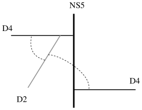
Figure 2: Brane construction of the unknot theory.

Moreover, the existence of a brane construction for this model was exploited in Hwang:2017kmk to derive a quiver description of the quantum mechanics of vortices for $T_{1}$, it is Quiver 1 in Figure 3. The circle represents a gauge group $U(n)$, the solid (resp. dashed) arrow represent a 1d ${\mathcal{N}}=2$ chiral (resp. Fermi) multiplet charged under $U(n)$, cf. (Hwang:2017kmk, , fig. 13). The Witten index computes the partition function of $n$ vortices, for a positive choice of the FI coupling it is given in (Hwang:2017kmk, , eq. (4.7))

$$I^{n}=a^{-n}q^{n}\frac{(a^{2};q^{2})_{n}}{(q^{2};q^{2})_{n}}\,.$$ (72)

The vortex partition function for theory $T_{1}$ is then

$$\mathcal{Z}^{\mathrm{vortex}}[T_{1}]=\sum_{n\geq 0}I^{n}\,x^{n}\dot{=}\sum_{n\geq 0}x^{n}\frac{(a^{2};q^{2})_{n}}{(q^{2};q^{2})_{n}}\,,$$ (73)

where for notational convenience we absorbed $a^{-1}q$ into the vortex fugacity by a redefinition $x\rightarrow a~{}q^{-1}x$, which is denoted by $\dot{=}$.

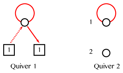
Figure 3: Quiver 1 encodes the ${\mathcal{N}}=2$ vortex quantum mechanics for the unknot theory $T[L_{K}]$. Quiver 2 encodes the ${\mathcal{N}}=4$ quantum mechanics of holomorphic disks and this is $Q_{0_{1}}$ analyzed in Section 5.1.

On the other hand, Quiver 2 coincides with the quiver $Q_{0_{1}}$ found in Kucharski:2017poe ; Kucharski:2017ogk . It describes a ${\mathcal{N}}=4$ quantum mechanics with gauge group $U(d_{1})\times U(d_{2})$ and an adjoint chiral multiplet charged under the first group. The refined Witten index $I^{\mathbf{d}}$ is zero for most dimension vectors $\mathbf{d}=(d_{1},d_{2})$, except for

$$I^{(1,0)}=-q\,,\qquad I^{(0,1)}=1\,.$$ (74)

These are the motivic DT invariants of the quiver representation theory, see Section 5.1. The corresponding motivic generating series gives the vortex partition function

$$\mathcal{Z}^{\mathrm{vortex}}[T_{2}]=\textrm{Exp}\left(\frac{I^{(1,0)}x_{1}+I^{(0,1)}x_{2}}{1-q^{2}}\right)=\sum_{d_{1},d_{2}\geq 0}(-q)^{d_{1}^{2}}\frac{x_{1}^{d_{1}}}{(q^{2};q^{2})_{d_{1}}}\frac{x_{2}^{d_{2}}}{(q^{2};q^{2})_{d_{2}}}\,.$$ (75)

The background Chern-Simons couplings $a_{i},t_{i},q_{i}$ of theory $T_{2}$ are

$$a_{1}=2\,,q_{1}=0\,,t_{1}=1\,,\qquad a_{2}=0\,,q_{2}=0\,,t_{2}=0\,.$$ (76)

These values instruct us to compare the two expressions through the following (KQ) change of variables:

$$x_{1}=xa^{2}q^{-1}\qquad x_{2}=x\,.$$ (77)

It is not hard to check that these relations imply

$$\mathcal{Z}^{\mathrm{vortex}}[T_{1}]=\mathcal{Z}^{\mathrm{vortex}}[T_{2}]\,.$$ (78)

Theories $T_{1}$ and $T_{2}$ have the same vortex spectrum, however this is described by two rather different quivers. In the first description there is a single gauge node, whose fugacity is $x$: this is the description that arises naturally from a brane construction Dimofte:2010tz ; Hwang:2017kmk where the $U(1)$ symmetry arises from $H_{1}(L_{K})\simeq{\mathbb{Z}}$. The quiver quantum mechanics arises from the equivariant localization of the path integral of the 3d-5d system, as a consequence its Witten index computes the $n$-vortex partition function. On the other hand, the second description involves two gauge groups which appear to be a mix of the gauge $U(1)$ appearing in $T_{1}$ with the background global symmetries. The precise combination of these $U(1)$’s is dictated precisely by $a_{i},q_{i},t_{i}$, recall (77). The Witten index of the second quiver does not give the vortex partition function, which is instead given by its plethystic exponential in (75). This is reminiscent of quiver descriptions of M2 boundstates in 4d ${\mathcal{N}}=2$ theories Denef:2002ru , providing another hint that the quiver quantum mechanics of theory $T_{2}$ describes the worldvolume dynamics of two basic holomorphic disks.

Another important distinction between the two quivers is the amount of supersymmetry involved in each description: Quiver 1 encodes an ${\mathcal{N}}=2$ quantum mechanics which is the expected description of vortices, while Quiver 2 describes a ${\mathcal{N}}=4$ quantum mechanics which is expected for a description of M2-branes ending on $L_{K}$ Aganagic:2012hs . This suggests that these dual descriptions can be regarded as switching the perspective from the dynamics of the M5-brane wrapped on $L_{K}$, to the dynamics of holomorphic disks that end on it. Indeed Quiver 1 arises naturally from the brane construction Dimofte:2010tz ; Hwang:2017kmk , while the origin of Quiver 2 is more naturally understood from the viewpoint of interacting holomorphic disks.

From the perspective of knot theory, it is clear that each node of the quiver must be dual to a generator of HOMFLY-PT homology (see Section 2.3). In turn, generators of the homology are dual to embedded holomorphic disks ending on $L_{K}$. Since $x_{i}\sim x$, these are the disks that wind exactly once around the generator of $H_{1}(L_{K})$. The rationale behind quiver descriptions of BPS spectra is that the quiver nodes are the “basic” BPS states, while the rest is generated from their boundstates. The latter consist of more complicated holomorphic curves, winding more than once around $L_{K}$ – generalized holomorphic curves introduced in Section 2.4 and further studied in Section 4. The quiver $Q_{K}$ encodes the dynamics of interacting basic disks, which determines the spectrum of their boundstates. In turn, this dynamics must depend on the geometry of the  M5-brane wrapping $L_{K}$: this is non-compact and rigid, providing a background on which the M2-branes wrapping holomorphic disks can end and interact with each other. This viewpoint is further corroborated by considering the Legendre transform of $T[Q_{K}]$: this gives an effective theory associated to $W_{Q_{K}}(\mathbf{x})$ (the quiver disk potential defined in (48)), which describes precisely the interaction of sources $x_{i}$ corresponding to basic holomorphic disks.

Interactions among basic disks may be encoded for example by the mutual linking numbers of disk boundaries. When two boundaries link, the M2 worldvolumes can interact, the light fields localized at the intersection of a family of Dirac strings beginning of one boundary and the other boundary give rise to $C_{ij}$ bifundamental modes (the quiver arrows) in the quiver quantum mechanics Denef:2002ru . A bit more precisely, while this picture is natural for mutual disk intersections (identified with $C_{ij}$) corresponding to M2-M2 interactions, more care is needed for self-linking (identified with $C_{ii}=t_{i}$). In fact this gets contribution from both M2-M2 self-interactions and M2-M5 interactions. For the example at hand, we can see this mixing appearing in the $q$-powers of (77): both $q_{1}=q_{2}=0$ are the same since both disks end on $L_{K}$ without linking (a proper mathematical definition of this will be given in the next section) and therefore both M2-branes have the same type of interaction with M5 wrapping $L_{K}$; on the other hand $t_{1}\neq t_{2}$ because one of the basic disks is self-linking, and therefore a BPS M2-brane wrapped on it experiences a nontrivial M2-M2 self-interaction.

4 KQ correspondence and geometry of holomorphic curves

In this section we discuss geometric interpretations of the knots-quivers correspondence. We first introduce necessary geometric objects, in particular generalized holomorphic curves. Then, we analyze the meaning of nodes and arrows from different perspectives. Finally, we study refinement in the context of LMOV invariants and geometry of Chern-Simons theory.

4.1 Quivers and generalized holomorphic curves

We give a geometric interpretation of the quiver vertices and arrows described in Section 2.4. The basic idea is that all holomorphic curves arise from a finite collection of basic holomorphic disks. Other holomorphic curves are then combinations of standard contributions from constant curves and branched covers of basic disks, and the quiver partition function arises as the corresponding count. For simple knots the basic disks correspond to the monomials in the HOMFLY-PT polynomial. In the general case, also other disks are needed and it is an open problem to give an effective characterization of when and how to find these additional disks.

As explained in Ekholm:2018iso , see also iacovino1 ; iacovino2 ; iacovino3 for similar earlier results, not only actual holomorphic curves, but also their composite configurations contribute to open Gromov-Witten potentials. Such configurations are called generalized holomorphic curves and to specify them we need additional geometric data that we decribe next. Before the description we point out that the generalized holomorphic curves generated by basic disks are closely related to $U(1)$ Chern-Simons theory on $L_{K}$ with defects, see ES for the exact relation.

We recall the definiton of generalized holomorphic curves with boundary on a knot conormal $L_{K}\subset X$ in the resolved conifold $X$, see Ekholm:2018iso . The additional geometric data are as follows: a Morse function $f\colon S^{1}\times\mathbb{R}^{2}\to\mathbb{R}$ and a $4$-chain $C$ with boundary $\partial C=2\cdot L_{K}$ and such that the normal vector fields of $C$ along $\partial C$ equals $\pm J\cdot\nabla f$, where $J$ is the almost complex structure. More precisely, we will use Morse functions that are small perturbations of Bott functions as follows. Consider a function on $S^{1}\times\mathbb{R}^{2}$ that is independent of the $S^{1}$ coordinate and has a unique non-degnerate minimum in each $\mathbb{R}^{2}$-fiber and with radial gradient near infinity. Thinking of $S^{1}\times\mathbb{R}^{2}$ as $L_{K}$, such a function has a minimum along the knot $K\subset L_{K}$ (the Bott-manifold) and gradient flow along the ${\mathbb{R}}^{2}$ fibers. After small perturbation by a Morse function on $K$ with two critical points, the resulting Morse function will have two critical points $\kappa_{0}$ of index $0$ and $\kappa_{1}$ of index $1$. The stable manifold $W^{\rm s}(\kappa_{1})$ of $\kappa_{1}$ is the knot and the unstable manifold $W^{\rm u}(\kappa_{1})$ is a fiber disk. We will use Morse functions $f\colon L_{K}\to\mathbb{R}$ of this form.

Figure 4: Morse flow defining the 4-chain $C$, shown inside $L_{K}$.

We use the Morse function $f$ to associate bounding chain $\sigma_{u}$ to holomorphic curve with boundary on $L_{K}$, $u\colon(\Sigma,\partial\Sigma)\to(X,L_{K})$, as follows. Let $\sigma_{u}^{\prime}$ denote the union of all flow lines starting on $u(\partial\Sigma)$. Then the intersection of $\sigma_{u}^{\prime}$ with a boundary torus $\Lambda_{K}$ of $L_{K}$ sufficiently close to infinity is a curve that represents a class $k\xi+n\eta$ where $\xi$ is the longitude and $\eta$ the meridian. Finally, define

$$\sigma_{u}=\sigma_{u}^{\prime}-n\cdot W^{\rm u}(\kappa_{1}).$$ (79)

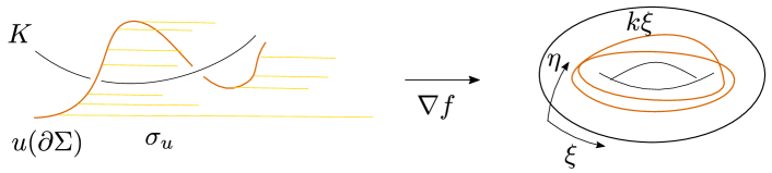
Figure 5: The bounding chain $\sigma_{u}$ ends on the cycle $k\xi$ on the torus at infinity inside $L_{K}$.

We also consider the following construction of an intrinsic self linking number of $u$. Let $\nu$ be any normal vector field of $\partial u$ and let $\partial u_{\nu}$ be a small shift of $\partial u$. We extend the vector field $J\nu$ to a small neighborhood of $\partial u$ and use that field to shift $u$ off of $L_{K}$. We denote the shifted curve $u_{J\nu}$ and define

$$\operatorname{slk}(u)=\partial u_{\nu}\cdot\sigma_{u}-u_{J\nu}\cdot C,$$ (80)

where $\cdot$ denotes algebraic intersection number. It is straightforward to check that $\operatorname{slk}(u)$ is independent of $\nu$: the first intersection number changes when $\nu$ passes $\pm\nabla f$ and a local check shows that there is then a compensating change in the second term.

Let us comment a bit more informally on the various ingredients that went into (80). On an intuitive level, the naive self-linking of a real curve $\partial u$ would be defined by first choosing a pushoff of $\partial u$ and then measuring the linking of the original curve with its pushoff. The pushoff is provided by $\nu$, while the linking may be defined as the meridian winding of the pushoff on the $T^{2}$ neighborhood of the original curve. The role of the Morse flow $\nabla f$ is to provide a notion of meridian winding for $\partial u$ around $K$, which would otherwise be topologically trivial in $L_{K}\sim S^{1}\times{\mathbb{R}}^{2}$. This information is encoded by the intersection of $\sigma_{u}^{\prime}$ with $\Lambda_{K}$, and eventually stored into the topology of the bounding chain $\sigma_{u}$ via (79). The meridian winding of the pushoff $\partial u_{\nu}$ is then its intersection with the bounding chain $\sigma_{u}$. The second piece in the formula accounts for the possibility that some of the self-intersections become “virtual”, such as through a Reidemeister zero-type move. The role of the four-chain is to collect these virtual contributions, and it is crucial that it is the imaginary counterpart of the Morse flow for this purpose.

A generalized holomorphic curve is a directed graph with actual holomorphic curves at the vertices. For each edge connecting two distinct curves $u$ and $v$ we pick an intersection point in $\partial u\cap\sigma_{v}$, and for each edge connecting a curve $u$ to itself we pick an intersection point contributing to $\operatorname{slk}(u)$. Such a generalized curve $\Gamma$ with vertices $V(\Gamma)$ and edges $E(\Gamma)$ is defined to have Euler characteristic

$$\chi(\Gamma_{u})=\sum_{u\in E(\Gamma)}\chi(u)-|E(\Gamma)|.$$ (81)

We next consider the relation to the quiver theory $T[Q_{K}]$. Let us assume that there is a finite number of embedded holomorphic disks with boundary on $L_{K}$, $u_{1},\dots,u_{m}$, where each $u_{j}$ has boundary that goes once around the generator of $H_{1}(L_{K})$. We assume furthermore that the linking numbers between holomorphic disk boundaries are

$$C_{ij}=\partial u_{i}\cdot\sigma_{u_{j}}=\partial u_{j}\cdot\sigma_{u_{i}},\quad C_{ii}=\partial{u_{i}}_{\nu}\cdot\sigma_{u_{i}},$$ (82)

where $\nu$ is the normal vector field everywhere linearly independent with $\nabla f$.

Note that for each embedded disk, the count of contributions from constant curves and multiple covers are exactly like for the basic disks for the unknot. We say that the generalized holomorphic curves that have vertices corresponding to branched covers and constant curves of the basic disks are the curves generated by the basic disks.

It then follows from the count of curves for the unknot, together with the definition of generalized holomorphic curves, that if $Q_{K}$ is the quiver with nodes $u_{1},\dots,u_{m}$ and associated quiver variables $x_{1},\dots,x_{m}$, and adjacency matrix $C_{ij}$, then the Gromov-Witten partition function that counts curves generated by the basic disks and the quiver generating function are equal (see (Ekholm:2018iso, , Section 2.4)), provided we make the substitution

$$x_{i}=x^{n_{i}}a^{a_{i}}q^{\operatorname{slk}(u_{i})-C_{ii}},$$ (83)

where $q=e^{\frac{1}{2}g_{s}}$. We will discuss this observation with more details and also including refinements of the count in the following sections.

We would like to close this section with a discussion of framing. The framing of $L_{K}$ corresponds to the choice of longitude curve in the torus at infinity which affects the definition of the bounding chain $\sigma_{u}$ of a holomorphic disk. More precisely, if $u$ is a basic holomorphic disk and the new longitude is $\xi+f\eta$, the bounding chain for $u$ is changed by addition of $f\cdot W^{\rm u}(\kappa_{1})$. Noting that the holomorphic curves themselves are unaffected by the choice of framing and that all basic disks go once around the homology generator, it follows from (82) that a framing change modifies the quiver by an overall additive constant $C_{ij}\to C_{ij}+f,$ adding $f$ arrows between all vertices. This matches indeed the description of framing found in Kucharski:2017poe ; Kucharski:2017ogk .

4.2 Contributions from quiver nodes

In this section we discuss various interpretations of quiver nodes including as homology generators, as LMOV invariants, and as basic holomorphic disks. Let us consider the quiver motivic generating series restricted to dimension vectors of length one:

$$P_{|\mathbf{d}|=1}^{Q_{K}}(\mathbf{x},q)=\sum_{i=1}^{m}\frac{(-q)^{C_{ii}}x_{i}}{1-q^{2}}\,.$$ (84)

Here every quiver vertex contributes, but there are no contributions from interactions between vertices since any resulting “bound states” give terms that are at least quadratic in the variables $x_{i}$.

If we apply the KQ change of variables, then we obtain the standard HOMFLY-PT polynomial (colored by the standard one box representation):

$$\left.P_{|\mathbf{d}|=1}^{Q_{K}}(\mathbf{x},q)\right|_{x_{i}=a^{a_{i}}q^{q_{i}-C_{ii}}x}=\ P_{1}^{K}(a,q)x\ =\ P_{1}^{K}(a,q)e^{\xi}\,.$$ (85)

We first observe a connection to HOMFLY-PT homology. As pointed out in Section 2.3, powers $a_{i}$, $q_{i}$, $t_{i}=C_{ii}$ are equal to degrees of natural generators of HOMFLY-PT homology $\mathscr{H}(K)$. More precisely, if $\mathscr{G}(K)$ denotes this set of generators then

$$P_{1}^{K}(a,q)=\frac{\sum_{i\in\mathscr{G}(K)}a^{a_{i}}q^{q_{i}}(-1)^{t_{i}}}{1-q^{2}}.$$ (86)

Following Kucharski:2017poe ; Kucharski:2017ogk , we consider also further refined versions of the KQ change of variables, corresponding to three and four gradings, and get

$$\begin{split}\left.P_{|\mathbf{d}|=1}^{Q_{K}}(\mathbf{x},q)\right|_{x_{i}=a^{a_{i}}q^{q_{i}-C_{ii}}(-t)^{C_{ii}}x}&=\ \mathcal{P}_{1}^{K}(a,q,t)x\ \\ &=\ \frac{\sum_{i\in\mathscr{G}(K)}a^{a_{i}}q^{q_{i}}t^{t_{i}}}{1-q^{2}}x\,,\end{split}$$ (87)

$$\begin{split}\left.P_{|\mathbf{d}|=1}^{Q_{K}}(\mathbf{x},q)\right|_{x_{i}=a^{a_{i}}Q^{q_{i}}(-t_{r})^{C_{ii}}x,\ q=t_{c}}&=\ \tilde{\mathcal{P}}_{1}^{K}(a,Q,t_{r},t_{c})x\\ &=\ \frac{\sum_{i\in\tilde{\mathscr{G}}(K)}a^{a_{i}}Q^{q_{i}}t_{r}^{t_{i}}t_{c}^{t_{i}}}{1-t_{c}^{2}}x\,.\end{split}$$ (88)

Comparing with Section 4.1 we see that the splitting of $q$ between $Q$, $t_{r}$, $t_{c}$ and other properties are perfectly consistent with geometric interpretation in terms of holomorphic disks:

• Each node corresponds to a holomorphic disk.

• The power $r=1$ in $x^{r}=e^{r\xi}$ corresponds to the homology class of the boundary of the holomorphic curve in $H_{1}(L_{K})$.

• After picking a reference disk $\delta$ capping the generator $\xi$ of $H_{1}(L_{K})$ the power $a_{i}$ in $a^{a_{i}}$ is the homology class of the holomorphic curve capped by $-r\delta$ in $H_{2}(X)$.

• The power $q_{i}$ in $Q^{q_{i}}$ is the self-linking $\textrm{slk}(u_{i})$.

• The exponent $t_{i}=C_{ii}$ in $t_{r}^{t_{i}}=t_{r}^{C_{ii}}$ equals the intersection number $\partial{u_{i}}_{\nu}\cdot\sigma_{u_{i}}$.

• The powers of $t_{c}$ are encoded in the off-diagonal entries in the adjacency matrix $C_{ij}$ and correspond to to the number of intersection points between $\partial u$ and $\sigma_{v}$: $C_{ij}=\partial u_{i}\cdot\sigma_{u_{j}}$.

In conclusion, we observe that there is a natural correspondence between basic holomorphic disks and topological data associated to them and homology generators and their degrees.

Since uncolored HOMFLY-PT homology is directly related to LMOV invariants GSV0412 , we can add another ingredient to our picture. Let us start by expressing (84) in terms of the DT generating function

$$P_{|\mathbf{d}|=1}^{Q_{K}}(\mathbf{x},q)=\frac{\Omega_{|\mathbf{d}|=1}^{Q_{K}}(\mathbf{x},q)}{1-q^{2}}\,.$$ (89)

After applying the KQ change of variables, we obtain

$$P_{1}^{K}(a,q)x=\frac{N_{1}^{K}(a,q)x}{1-q^{2}}\,.$$ (90)

LMOV invariants count BPS states in 3d $\mathcal{N}=2$ theory $T[L_{K}]$ described in Section 3.1, whereas DT invariants give numbers of BPS states in 3d $\mathcal{N}=2$ theory $T[Q_{K}]$ from Section 3.3. Therefore we can reinterpret our holomorphic disks and their topological data in terms of BPS states and their quantum numbers. This is in line with the brane construction from Ooguri:1999bv . $T[L_{K}]$ arises as effective theory on the surface of M5-brane and its BPS particles originate from M2-branes ending on M5, which brings us back to holomorphic disks ending on the Lagrangian submanifold. Here it is natural to interpret the adjacency matrix $C_{ij}$ as corresponding to M2-M2 interactions and the parameter $q_{i}-C_{ii}$ as corresponding to M2-M5 interactions.

Looking back at equations (89–90), we can ask what happens if we apply refined KQ changes of variables. We will come back to this question in Section 4.4.

In this section we were dealing with different interpretations of quiver nodes. They correspond to holomorphic disks, homology generators and BPS states. The KQ change of variables can be encoded in topological data of disks, degrees of generators, or quantum numbers of BPS states. Let us stress that we considered dimension vectors of lenght one, which corresponds to fundamental representation or disks winding around $L_{K}$ once. In this case there is no interaction between nodes, so all observations from this section can be summarized as describing internal properties of considered objects. (Here internal should be understood as involving M2 self interactions and M2-M5 interactions.)

4.3 Arrows: how basic disks generate all curves

After considering internal properties of objects corresponding to quiver nodes, we are ready to look at their interactions encoded in quiver arrows.

The motivic generating series is built by combinations of factors from the nodes determined by dimension vector $\mathbf{d}$ and weighted according to the adjacency matrix $C_{ij}$

$$P^{Q}(\mathbf{x},q)=\sum_{d_{1},\ldots,d_{m}\geq 0}(-q)^{\sum_{1\leq i,j\leq m}C_{ij}d_{i}d_{j}}\prod_{i=1}^{m}\frac{x_{i}^{d_{i}}}{(q^{2};q^{2})_{d_{i}}}.$$ (91)

The KQ change of variables hides this structure, but does not break it

$$\left.P^{Q_{K}}(\mathbf{x},q)\right|_{x_{i}=a^{a_{i}}q^{q_{i}-C_{ii}}x} =P^{K}(x,a,q)$$ (92)

$$=\sum_{d_{1},\ldots,d_{m}\geq 0}(-q)^{\sum_{1\leq i,j\leq m}C_{ij}d_{i}d_{j}}\prod_{i=1}^{m}\frac{(a^{a_{i}}q^{q_{i}-C_{ii}}x)^{d_{i}}}{(q^{2};q^{2})_{d_{i}}}.$$

We then see that quiver arrows encode the way of building the whole spectrum of objects (counted by the motivic generating series or the HOMFLY-PT generating function) from the basic ones which correspond to nodes.

Interpreting the nodes as holomorphic disks we find that the adjacency matrix exactly encodes how to build all generalized holomorphic curves from the basic disks. The dimension vector encodes the number of copies of the disk, the matrix $C_{ij}$ counts in how many ways the various curves can be combined into generalized curves, and the transformations of self linking and topological degrees behaves in accordance with this interpretation.

In fact, the quiver partition function counts all disconnected generalized holomorphic curves generated by the basic disks $u$. To see this, we first note that all embedded disks have a standard neighborhood and then we can infer the count of multiple covers and contributions from constant curves attached to these from that of disks on the unknot, where we have the recursion that determines the factors. The contributions from linking and self-linking follows from the description of generalized holomorphic curves above.

The holomorphic disks corresponding to the nodes of the quiver are embedded. Generalized holomorphic curves are constructed in order for the count of all curves to remain invariant under deformations. One can also consider the counts of generalized embedded disks. Basically, new embedded disks appear when two embedded disks intersect along the boundary. Therefore, in order to count these objects we should count trees of nodes and arrows rather than arbitrary graphs. We call such generalized holomorphic curves semi-basic disks. Arguing as above, we then find that the generating function of semi-basic disks equals the DT generating function, i.e. the count of BPS states of the quiver.

Looking at (5) and (52) we can see that generalized holomorphic curves counted by quiver partition function are generated by basic disks in the “sum way” or characterized by semi-basic disks leading to a partition function written in the “product way”. From the point of view of states in $T[Q_{K}]$ we would say that all states are generated by basic states (those corresponding to $|\textbf{d}|=1$) in the “sum way” or associated to BPS states that give the partition function in the “product way”.

A similar distinction on the knot side was described in KS1608 using combinatorics on words. The “sum way” means direct generation of all words in a given formal language, whereas the the “product way” is represented by obtaining all words by concatenation of Lyndon words. We shall stress that the analogy is not perfect because in KS1608 the analysed generating fuction was the ratio $P^{K}(q^{2}x,a,q)/P^{K}(x,a,q)$, not the HOMFLY-PT generating series itself. However, the main structure is preserved, only building blocks are different. In our case they are basic disks corresponding to terms in $P^{K}_{1}(a,q)$, whereas in KS1608 they are one-letter words representing terms in the quantum A-polynomial.

Let us consider consequences of the result on generated holomorphic curves for the relation between the size of colored and uncolored homology. Since the KQ correspondence relates quiver nodes with generators of $\tilde{\mathscr{H}}(K)$ and quiver partition function with Poincaré polynomial of $\tilde{\mathscr{H}}^{S^{r}}(K)$, we can translate the generation of all generalized holomorphic curves by the basic disks to the exponential growth property Gukov:2011ry ; GGS1304 ; Wed1602

$$\dim\tilde{\mathscr{H}}^{S^{r}}(K)=\left(\dim\tilde{\mathscr{H}}(K)\right)^{r}\,.$$ (93)

This statement shows limitations of the KQ correspondence with quiver nodes corresponding to generators of $\tilde{\mathscr{H}}(K)$. In Section 6.1 we study the case of the knot $9_{42}$ which does not have this property and discuss possible generalizations of Kucharski:2017poe ; Kucharski:2017ogk that would cure this problem.

4.4 Quiver-based refinement of LMOV invariants

Let us recall the relation between LMOV invariants of a knot $K$ and DT invariants of the corresponding quiver $Q_{K}$:

$$N^{K}(x,a,q)=\left.\Omega^{Q_{K}}(\mathbf{x},q)\right|_{x_{i}=a^{a_{i}}q^{q_{i}-C_{ii}}x}\,.$$ (94)

As suggested in Kucharski:2017poe ; Kucharski:2017ogk , we can define refined LMOV invariants by applying the refined KQ change of variables to $\Omega^{Q_{K}}(\mathbf{x},q)$:

$$N^{K}(x,a,q,t)=\sum_{r,i,j,k}N_{r,i,j,k}^{K}x^{r}a^{i}q^{j}t^{k}=\left.\Omega^{Q_{K}}(\mathbf{x},q)\right|_{x_{i}=a^{a_{i}}q^{q_{i}-C_{ii}}(-t)^{C_{ii}}x}\,.$$ (95)

Applying the plethystic exponential to this formula gives the generating function of unreduced superpolynomials:

$$\textrm{Exp}\left(\frac{N^{K}(x,a,q,t)}{1-q^{2}}\right) =\left.\textrm{Exp}\left(\frac{\Omega^{Q_{K}}(\mathbf{x},q)}{1-q^{2}}\right)\right|_{x_{i}=a^{a_{i}}q^{q_{i}-C_{ii}}(-t)^{C_{ii}}x}$$

$$=\left.P^{Q_{K}}(\mathbf{x},q)\right|_{x_{i}=a^{a_{i}}q^{q_{i}-C_{ii}}(-t)^{C_{ii}}x}$$ (96)

$$=\mathcal{P}^{K}(x,a,q,t).$$

Since for symmetric quivers DT invariants are integer 2011arXiv1103.2736E , the integrality of refined LMOV invariants defined in this way holds by definition. In the limit $q\rightarrow 1$ they reduce to classical refined LMOV invariants introduced in GKS1504 (see Section 5 for examples and Appendix A for comparison of conventions). A slightly different refinement was proposed in KN1703 where $t_{c}$ is used as $t$ instead of $t_{r}$.

These two possibilities of consistent refinement of HOMFLY-PT homology was in fact one of the sources of inspiration for introducing a quadruply graded homology in GGS1304 . Our framework also enables a natural definition of doubly refined LMOV invariants:

$$\begin{split}N^{K}(x,a,Q,t_{r},t_{c})&=\sum_{r,i,j,k,l}N_{r,i,j,k,l}^{K}x^{r}a^{i}Q^{j}t_{r}^{k}t_{c}^{l}\\ &=\left.\Omega^{Q_{K}}(\mathbf{x},q)\right|_{x_{i}=a^{a_{i}}Q^{q_{i}}(-t_{r})^{C_{ii}}x,\ q=t_{c}}\end{split}$$ (97)

In this case the plethystic exponential gives the generating function of unreduced quadruply-graded polynomials:

$$\textrm{Exp}\left(\frac{N^{K}(x,a,Q,t_{r},t_{c})}{1-q^{2}}\right) =\left.\textrm{Exp}\left(\frac{\Omega^{Q_{K}}(\mathbf{x},q)}{1-q^{2}}\right)\right|_{x_{i}=a^{a_{i}}Q^{q_{i}}(-t_{r})^{C_{ii}}x,\ q=t_{c}}$$

$$=\left.P^{Q_{K}}(\mathbf{x},q)\right|_{x_{i}=a^{a_{i}}Q^{q_{i}}(-t_{r})^{C_{ii}}x,\ q=t_{c}}$$ (98)

$$=\sum_{d_{1},\ldots,d_{m}\geq 0}(-t_{c})^{\sum_{1\leq i,j\leq m}C_{ij}d_{i}d_{j}}\prod_{i=1}^{m}\frac{(a^{a_{i}}Q^{q_{i}}t_{r}^{C_{ii}}x)^{d_{i}}}{(t_{c}^{2};t_{c}^{2})_{d_{i}}}$$

$$=\mathcal{\tilde{P}}^{K}(x,a,Q,t_{r},t_{c}).$$

Note that the form of the motivic generating function induces the $(t_{c}^{2};t_{c}^{2})_{r}$ denominator of $\mathcal{\tilde{P}}_{r}^{K}$, which is the source of the nonstandard definition in Section 2.3.

Explicit calculations of refined and doubly refined LMOV invariants for the unknot and the trefoil are presented in Section 5.1 and 5.2 respectively.

4.5 The geometry of refined Chern-Simons

In this section we discuss the geometry of refined Chern-Simons theory. Our approach is closely related to that of Aganagic:2012hs . We will also indicate how this relates to self linking and 4-chain intersections above. The details of that depend on ES and will not be fully discussed here.

Let $K=K_{1}\cup\dots\cup K_{n}$ be an $n$-component link and let $L_{K}=L_{K_{1}}\cup\dots\cup L_{K_{n}}$ be its Lagrangian conormal considered as a Lagrangian submanifold of the resolved conifold as above. We will consider holomorphic curves with boundary on $L_{K}$. As above they are all rigid. We apply Symplectic Field Theory stretching near each component of $L_{K}$. We fix a metric on the components of $L_{K}$ (topology $S^{1}\times\mathbb{R}^{2}$) with exactly one closed geodesic $S^{1}\times 0$. Under such stretching, the curves subdivide into components in the complement $X\backslash L_{K}$ asymptotic to multiples of the Reeb orbit which is the lift of multiples of the geodesic, and components on the inside also asymptotic to the Reeb orbits and with boundary on the $0$-section. A straightforward index argument shows that the count of curves in the complement with fixed asymptotics is invariant under deformations. Fixing a capping disk in $X\backslash L_{K}$ (which is simply connected) for each Reeb orbit we cap each holomorphic curve to a 2-cycle in $X\backslash L_{K}$.

A straightforward calculation shows that

$$H_{2}(X\backslash L_{K})=\mathbb{Z}[\mathbb{C}{\mathbb{P}}^{1}]\oplus\mathbb{Z}[S_{1}]\oplus\dots\oplus\mathbb{Z}[S_{n}],$$ (99)

where $S_{j}$ is the fiber 2-sphere in the boundary of a tubular neihgborhood of $L_{K_{j}}$. This gives a refined Gromov-Witten potential:

$$\Psi_{K}(a,a_{(1)},\dots,a_{(n)}),$$ (100)

where $a_{(j)}$ keeps track of the homology class (it is not $a_{i}$ from the KQ change of variables).

For calculations from infinity, it is useful to glue back the curves and consider curves with boundaries. Following ES , we should view the Gromov-Witten invariant as taking values in the skein module of $L_{K}$, where $(a_{(j)},q)$ are the variables in the skein module of $L_{K_{j}}$ and $q=e^{\frac{1}{2}g_{s}}$. This is a useful perspective since it allows for using Legendrian SFT at infinity to compute the refined Schrödinger equation by elimination as for the unrefined colored HOMFLY-PT in Ekholm:2018iso . From this perspective, the refined partition function corresponds to $U(1)$ Chern-Simons theory on $L_{K}$, which means that $a_{(j)}=q$ and refinement concern a splitting of this $q$-variable into $q$ and $t$, where one $t$ corresponds to the self-linking of the boundary of the holomorphic disk and the other $q$ accounts for genus and for $4$-chain intersections. The exact nature of this splitting is not yet understood.

We end this section with a discussion of the distinctions between the refinements $t_{c}$ and $t_{r}$ above. Here the variable $t_{c}$ is related to linking (and self-linking) between boundaries of holomorphic curves inside $L_{K}$ and is hence an effect of M2-M2 interactions. The variable $t_{r}$ on the other hand counts intersections with the $4$-chain and is thus an effect of M2-M5 interactions. Looking at the curves generated by a given set of disks, it is clear that one transforms quadratically and the other linearly in the number of disks in a boundstate (the dimension vector ${\mathbf{d}}$).

5 Examples

In this section we present the ideas and interpretations described in Sections 3 and 4 with explicit examples of knots and corresponding quivers. Since every case demands a long discussion, we will focus on the two simplest ones: the unknot and the trefoil.

5.1 Unknot

According to the KQ correspondence Kucharski:2017poe ; Kucharski:2017ogk , the unknot quiver contains two nodes and one loop:

$$Q_{0_{1}}=\raisebox{-21.52771pt}{\includegraphics[width=43.36464pt]{unknot-KRSSquiver.pdf}}\qquad\Longleftrightarrow\qquad C=\left[\begin{array}[]{cc}1&0\\ 0&0\end{array}\right]\,.$$ (101)

The motivic generating series is therefore given by

$$P^{Q_{0_{1}}}(\mathbf{x},q)=\sum_{d_{1},d_{2}\geq 0}(-q)^{d_{1}^{2}}\frac{x_{1}^{d_{1}}}{(q^{2};q^{2})_{d_{1}}}\frac{x_{2}^{d_{2}}}{(q^{2};q^{2})_{d_{2}}}\,.$$ (102)

Note that in order to compare with formulas in Kucharski:2017poe ; Kucharski:2017ogk one has to substitute $x_{i}\rightarrow qx_{i}$. On the other hand, PSS1802 uses the same convention as we do.

Since

$$P^{Q_{0_{1}}}(\mathbf{x},q)= \textrm{Exp}\left(\frac{\Omega^{Q_{0_{1}}}(\mathbf{x},q)}{1-q^{2}}\right)\,,$$ (103)

$$\textrm{Exp}\left(\frac{-qx_{1}+x_{2}}{1-q^{2}}\right)= \textrm{Exp}\left(\frac{\sum_{\mathbf{d},s}\Omega_{\mathbf{d},s}^{Q_{0_{1}}}\mathbf{x}^{\mathbf{d}}q^{s}(-1)^{|\mathbf{d}|+s+1}}{1-q^{2}}\right)\,,$$

we have only two nonzero DT invariants

$$\Omega_{(1,0),1}^{Q_{0_{1}}}=1\,,\qquad\Omega_{(0,1),0}^{Q_{0_{1}}}=1\,,$$ (104)

and numerical DT invariants

$$\Omega_{(1,0)}^{Q_{0_{1}}}=-1\,,\qquad\Omega_{(0,1)}^{Q_{0_{1}}}=1\,.$$ (105)

All of them correspond to $\mathbf{|d|}=1$, so for $T[Q_{0_{1}}]$ all BPS states are basic states.

The KQ change of variables

$$x_{1}=a^{2}q^{-1}x,\qquad x_{2}=x$$ (106)

translates the motivic generating series to the (unreduced) HOMFLY-PT generating series of the unknot:

$$\left.P^{Q_{0_{1}}}(\mathbf{x},q)\right|_{x_{1}=a^{2}q^{-1}x,\;x_{2}=x}= P^{0_{1}}(x,a,q)$$ (107)

$$= \sum_{r=0}^{\infty}\frac{(a^{2};q^{2})_{r}}{(q^{2};q^{2})_{r}}x^{r}\,,$$

which confirms (101). Note that in the knot theory literature (including Kucharski:2017poe ; Kucharski:2017ogk ) usually there is a prefactor $a^{-r}q^{r}$ before $\frac{(a^{2};q^{2})_{r}}{(q^{2};q^{2})_{r}}$ in $P_{r}^{0_{1}}(a,q)$ and often (e.g. in Fuji:2012nx ) $a^{1/2}$ and $q^{1/2}$ are used instead of $a$ and $q$. Our convention is designed for the most natural description of knots-quivers correspondence.

We next look at this calculation from the point of view of holomorphic disks. We first note that from the toric picture of the unknot conormal it is clear that there are two basic holomorphic disks Ooguri:1999bv . Furthermore, we see from the HOMFLY-PT polynomial that they contribute the same to generalized holomorphic disk. The only point that remains to explain is the difference in $t$-powers, or in other words the difference between $C_{00}$ and $C_{11}$. To explain this, we look at moduli spaces of curves with one positive puncture, as in knot contact homology. At infinity there are four such disks in homology classes $1$, $e^{\eta}$, $e^{\xi}$, and $a^{2}e^{\xi}e^{\eta}$ (these are the terms in the operator equation (23)). By the main result of ES , the boundary of holomorphic disks in the skein module does not change under deformation provided the skein variable $(q,t)$ satisfies $q=e^{\frac{1}{2}g_{s}}$, and that 4-chain intersections contribute $t^{\pm 1}$. The deformation invariance then implies that the boundaries of a 1-dimensional moduli space equals zero in the skein module. This can then be used to understand relevant boundaries of holomorphic disks.

We use this argument here. First, consider the disks with boundaries that represent the trivial class in $H_{1}(L_{K})$. There are two such curves $1$ and $e^{\eta}$ that come with opposite signs and hence cancel in the skein module of $L_{K}$. Consider next the disks that goes once around the generator and represent the trivial homology class in $H_{2}(X)$. There are then the disks $e^{\xi}$ at infinity and the disks $e^{\eta}\cdot u_{0}$, see Ekholm:2018iso . The corresponding disks for $a^{2}$ are $a^{2}e^{\eta}e^{\xi}$ at infinity and $e^{\eta}\cdot u_{1}$. Write the boundary of the basic disk with minimal $a$ power $u_{0}$ in the skein module as $p(q,t)\cdot e^{\xi}$, where we think of $e^{\xi}$ as the standard longitude with one twist. Then, using the skein relation (note that ES uses the skein relation with $q-q^{-1}$ instead of $1-q^{2}$) we have

$$(1-e^{\eta})e^{\xi}=(1-q^{2})e^{\xi}$$

and we find that $u_{0}=\frac{1}{1-q^{2}}$. The only difference in the calculation for the maximal disk is that $e^{\xi}$ is replaced by the disk $e^{\xi}e^{\eta}=te^{\xi}$ and we get $u_{1}=\frac{t}{1-q^{2}}$. It follows that $C_{11}=C_{00}+1$.

Homologies and BPS states

Generators of uncolored HOMFLY-PT homology $\mathscr{H}(0_{1})$, i.e. elements of $\mathscr{G}(0_{1})$, have degrees given by the following vectors:

$$\mathbf{a}= (a_{1},a_{2})=(2,0)\,,$$

$$\mathbf{q}= (q_{1},q_{2})=(0,0)\,,$$ (108)

$$\mathbf{t}= (t_{1},t_{2})=(1,0)\,.$$

On the other hand, the application of KQ change of variables to $\mathbf{|d|}=1$ restriction of (102) leads to

$$\left.P_{|\mathbf{d}|=1}^{Q_{0_{1}}}(\mathbf{x},q)\right|_{x_{1}=a^{2}q^{-1}x,\ x_{2}=x}=\frac{1-a^{2}}{1-q^{2}}x=\frac{\sum_{i\in\mathscr{G}(0_{1})}a^{a_{i}}q^{q_{i}}(-1)^{t_{i}}}{1-q^{2}}x\,,$$ (109)

which shows a perfect consistency. Note that all comments about HOMFLY-PT conventions apply to degrees of $\mathscr{H}(0_{1})$ as well.

We can apply KQ change of variables also to the DT generating function in order to obtain the LMOV generating function:

$$\left.\Omega^{Q_{0_{1}}}(\mathbf{x},q)\right|_{x_{1}=a^{2}q^{-1}x,\;x_{2}=x}= N^{0_{1}}(x,a,q)$$ (110)

$$x-a^{2}x= \sum_{r,i,j}N_{r,i,j}^{0_{1}}x^{r}a^{i}q^{j}\,,$$

which leads to

$$N_{1,0,0}^{0_{1}}=1\,,\qquad N_{1,2,0}^{0_{1}}=-1\,.$$ (111)

Classical LMOV invariants are therefore given by

$$b_{1,0}^{0_{1}}=1\,,\qquad b_{1,2}^{0_{1}}=-1\,.$$ (112)

The shift in $a$ variable with respect to usual knot theory conventions (e.g. KS1608 ) comes from the lack of $a^{-r}q^{r}$ prefactor in $P_{r}^{0_{1}}(a,q)$. In $q$ variable this effect is compensated by $1-q^{2}$ denominator in the definition of the LMOV generating function (4), instead of the usual $q-q^{-1}$ present e.g. in KS1608 , so at the end of the day only the sign flip remains.

We can consider also the refined KQ change of variables:

$$x_{1}=a^{2}q^{-1}(-t)x,\qquad x_{2}=x$$ (113)

which translates the motivic generating series to the generating series of superpolynomials:

$$\left.P^{Q_{0_{1}}}(\mathbf{x},q)\right|_{x_{1}=a^{2}q^{-1}(-t)x,\ x_{2}=x}= \mathcal{P}^{0_{1}}(x,a,q,t)$$ (114)

$$= \sum_{r=0}^{\infty}\frac{(-a^{2}t;q^{2})_{r}}{(q^{2};q^{2})_{r}}x^{r}\,.$$

Restriction to $\mathbf{|d|}=1$ shows consistency of refined KQ change of variables with degrees of $\mathscr{H}(0_{1})$ given in (108):

$$\left.P_{|\mathbf{d}|=1}^{Q_{0_{1}}}(\mathbf{x},q)\right|_{x_{1}=a^{2}q^{-1}(-t)x,\ x_{2}=x}=\frac{1+a^{2}t}{1-q^{2}}x=\frac{\sum_{i\in\mathscr{G}(0_{1})}a^{a_{i}}q^{q_{i}}t^{t_{i}}}{1-q^{2}}x\,.$$ (115)

Applying refined KQ change of variables to the DT generating function we obtain

$$\left.\Omega^{Q_{0_{1}}}(\mathbf{x},q)\right|_{x_{1}=a^{2}q^{-1}(-t)x,\ x_{2}=x}= N^{0_{1}}(x,a,q,t)$$ (116)

$$x+a^{2}tx= \sum_{r,i,j}N_{r,i,j,k}^{0_{1}}x^{r}a^{i}q^{j}t^{k}\,,$$

so refined LMOV invariants read

$$N_{1,0,0,0}^{0_{1}}=1\,,\qquad N_{1,2,0,1}^{0_{1}}=1\,.$$ (117)

This is consistent with GKS1504 after taking into accout the fact that they use the convention of Fuji:2012nx for the $t_{r}$ refinement, with an extra $(-a^{-2}q^{2}t^{-3})^{r/2}$ prefactor, and use $a^{2}t^{3}$ instead of $a^{2}t$. These prefactors were introduced to provide more symmetric expressions – we drop them in order to obtain the KQ correspondence in a natural way. Our choice of $a^{2}t$ in $\mathcal{P}_{r}^{0_{1}}(a,q,t)$ is consistent with conventions of GGS1304 and GNSSS1512 on the $t_{r}$ refinement. The $t_{c}$ refinement adopted in KN1703 introduces $(q^{2};q^{2}t^{2})_{r}$ in the denominator, which is inconsistent with the form of the motivic generating series.

We can generalize our results to both $t_{r}$ and $t_{c}$ by considering doubly refined KQ change of variables:

$$x_{1}=a^{2}(-t_{r})x\,,\qquad x_{2}=x\,,\qquad q=t_{c}\,.$$ (118)

It translates the motivic generating series to the generating series of quadruply-graded polynomials:

$$\left.P^{Q_{0_{1}}}(\mathbf{x},q)\right|_{x_{1}=a^{2}(-t_{r})x,\ x_{2}=x,\ q=t_{c}}= \tilde{\mathcal{P}}^{0_{1}}(x,a,Q,t_{r},t_{c})$$ (119)

$$= \sum_{r=0}^{\infty}\frac{(-a^{2}t_{r}t_{c};t_{c}^{2})_{r}}{(t_{c}^{2};t_{c}^{2})_{r}}x^{r}\,.$$

Note that in GGS1304 and GNSSS1512 there is a $a^{-r}Q^{r}$ prefactor and $(Q^{2};t_{c}^{2})_{r}$ in the denominator. This discrepancy is analogous to the one with KN1703 and is forced by demanding consistency with the motivic generating series.

The doubly refined KQ change of variables is consistent with degrees of generators of the quadruply-graded homology $\tilde{\mathscr{H}}(0_{1})$. We can see it by comparing (108) to the $\mathbf{|d|}=1$ restriction of (119):

$$\left.P_{|\mathbf{d}|=1}^{Q_{0_{1}}}(\mathbf{x},q)\right|_{x_{1}=a^{2}(-t_{r})x,\ x_{2}=x,\ q=t_{c}}=\frac{1+a^{2}t_{r}t_{c}}{1-t_{c}^{2}}x=\frac{\sum_{i\in\tilde{\mathscr{G}}(0_{1})}a^{a_{i}}Q^{q_{i}}t_{r}^{t_{i}}t_{c}^{t_{i}}}{1-q^{2}}x\,.$$ (120)

Note that for uncolored homology degrees of $t_{r}$ and $t_{c}$ are the same, so they are both given by the vector $\mathbf{t}$ from (108). All comments about quadruply-graded polynomial conventions apply to degrees of $\tilde{\mathscr{H}}(0_{1})$ as well.

According to our reasoning from Section 4.4, we can define doubly refined LMOV invariants by applying (118) to the DT generating function:

$$\left.\Omega^{Q_{0_{1}}}(\mathbf{x},q)\right|_{x_{1}=a^{2}(-t_{r})x,\ x_{2}=x,\ q=t_{c}}= N^{0_{1}}(x,a,Q,t_{r},t_{c})$$ (121)

$$x+a^{2}t_{r}t_{c}x= \sum_{r,i,j,k,l}N_{r,i,j,k,l}^{0_{1}}x^{r}a^{i}Q^{j}t_{r}^{k}t_{c}^{l}\,,$$

which leads to

$$N_{1,0,0,0,0}^{0_{1}}=1\,,\qquad N_{1,2,0,1,1}^{0_{1}}=1\,.$$ (122)

3d $\mathcal{N}=2$ theories

As discussed in Section 3, we can use the generating series of superpolynomials and the motivic generating series to obtain twisted superpotentials of $T[L_{0_{1}}]$ and $T[Q_{0_{1}}]$ theories, whose BPS states are counted by LMOV and DT invariants respectively. Before considering them, let us follow Section 3.1 and focus on the theory $T_{0}[L_{0_{1}}]$. It is obtained from the limit (27), which for the unknot reads

$$\mathcal{P}_{r}^{0_{1}}(a,q,t)\underset{q^{2r}\rightarrow y}{\overset{\hbar\rightarrow 0}{\longrightarrow}}\exp\left[\frac{1}{2\hbar}\left(\widetilde{\mathcal{W}}_{T_{0}[L_{0_{1}}]}(a,t,y)+O(\hbar)\right)\right],$$ (123)

$$\widetilde{\mathcal{W}}_{T_{0}[L_{0_{1}}]}(a,t,y)=\textrm{Li}_{2}\left(y\right)-\textrm{Li}_{2}\left(-a^{2}ty\right)+\textrm{Li}_{2}\left(-a^{2}t\right)\,.$$

We can compare the above expression with the twisted superpotential for the knot complement theory in Fuji:2012nx . After changing variables $y\rightarrow x,\;a^{2}\rightarrow a,\;q^{2}\rightarrow q$, taking into account the fact that they have a $(-a^{-1}qt^{-3})^{r/2}$ prefactor and $-t^{3}$ instead of $-t$ in the $q$-Pochhammer, and noting that we have dropped the irrelevant $\textrm{Li}_{2}\left(1\right)$ term, we can see that they are consistent.

The moduli space of vacua of $T_{0}[L_{0_{1}}]$ is described by the zero-locus of the super-A-polynomial. According to (30), it is given by

$$\log x^{-1}=\frac{\partial\widetilde{\mathcal{W}}_{T_{0}[L_{0_{1}}]}(a,t,y)}{\partial\log y}=-\log(1-y)+\log(1+a^{2}ty)$$ (124)

so

$$\mathcal{A}^{0_{1}}(x,y,a,t)=1-x-y-a^{2}txy=0.$$ (125)

Note that according to terminology of KS1608 ; GKS1504 , $\mathcal{A}^{0_{1}}(x,y,a,t)$ is a dual super-A-polynomial, so in order to compare with a super-A-polynomial from Fuji:2012nx we have to change variables $y\rightarrow x,\;x\rightarrow y^{-1}$. Of course we have to include other conventional differences which were already discussed, namely add the prefactor $(-a^{-1}t^{-3})^{1/2}$ and change the term $a^{2}t$ to $at^{3}$. Comparison of (125) with dual A-polynomials from KS1608 ; GKS1504 demands only usual restriction $t=-1$ and rescaling $x\rightarrow a^{-1}x$.

We can obtain theory $T[L_{0_{1}}]$ by considering the generating function of superpolynomials. In the case of the unknot the limit (31) reads

$$\mathcal{P}^{0_{1}}(x,a,q,t)\underset{q^{2r}\rightarrow y}{\overset{\hbar\rightarrow 0}{\longrightarrow}}\int dy\exp\left[\frac{1}{2\hbar}\left(\widetilde{\mathcal{W}}_{T[L_{0_{1}}]}(a,t,x,y)+O(\hbar)\right)\right]$$ (126)

$$\widetilde{\mathcal{W}}_{T[L_{0_{1}}]}(a,t,x,y)=\textrm{Li}_{2}\left(y\right)-\textrm{Li}_{2}\left(-a^{2}ty\right)+\textrm{Li}_{2}\left(-a^{2}t\right)+\log x\log y$$

This twisted superpotential corresponds to $U(1)$ gauge theory with one fundamental chiral and one antifundamental chiral as it was noted in Section 3.5. Comparing (126) with (123), we can see that $U(1)_{M}$ symmetry corresponding to fugacity $y$ is gauged and there is an extra Fayet-Ilioupoulos term $\log x\log y$, which is line with (35). It also confirms that the weak coupling limit of $T[L_{0_{1}}]$ is $T_{0}[L_{0_{1}}]$.

Since for the unknot there are no gauge fuacities other than $y$ (denoted by $z_{i}$ in Section 3.1), we have

$$\widetilde{\mathcal{W}}_{T[L_{0_{1}}]}^{\textrm{eff}}(a,t,x,y) =\widetilde{\mathcal{W}}_{T[L_{0_{1}}]}(a,t,x,y)\,,$$ (127)

$$\widetilde{\mathcal{W}}_{T_{0}[L_{0_{1}}]}^{\textrm{eff}}(a,t,y) =\widetilde{\mathcal{W}}_{T_{0}[L_{0_{1}}]}(a,t,y)\,.$$

According to (40), we can obtain the Gromov-Witten disk potential $W_{0_{1}}$ as a Legendre transform of $\widetilde{\mathcal{W}}_{T_{0}[L_{0_{1}}]}$. It is equivalent to integrating out $y$ in $\widetilde{\mathcal{W}}_{T[L_{0_{1}}]}$, which can be done by saddle-point approximation. Solving

$$0=\frac{\partial\widetilde{\mathcal{W}}_{T[L_{0_{1}}]}(a,t,x,y)}{\partial\log y}=-\log(1-y)+\log(1+ya^{2}t)+\log x$$ (128)

we obtain

$$y^{*}(x)=\frac{1-x}{1+a^{2}tx}\,,$$ (129)

which is equivalent to the super-A-polynomial (125). Therefore

$$W_{0_{1}}(a,x)= \left.\left(\widetilde{\mathcal{W}}_{T_{0}[L_{0_{1}}]}(a,t,y)+\log y\log x\right)\right|_{y^{*}(x),\ t=-1}$$

$$= \left.\widetilde{\mathcal{W}}_{T[L_{0_{1}}]}(a,t,x,y)\right|_{y^{*}(x),\ t=-1}$$ (130)

$$= \textrm{Li}_{2}\left(\frac{1-x}{1-a^{2}x}\right)-\textrm{Li}_{2}\left(\frac{a^{2}-a^{2}x}{1-a^{2}x}\right)+\textrm{Li}_{2}\left(a^{2}\right)+\log x\log\left(\frac{1-x}{1-a^{2}x}\right)$$

$$= \textrm{Li}_{2}\left(a^{2}x\right)-\textrm{Li}_{2}\left(x\right)\,,$$

where we used the pentagon relation for dilogarithms. As a cross-check let us calculate the Gromov-Witten disk potential from classical LMOV invariants (112) using (58). We obtain

$$W_{0_{1}}(a,x)=\left(-b_{1,0}^{0_{1}}\right)\textrm{Li}_{2}\left(x^{1}a^{0}\right)+\left(-b_{1,2}^{0_{1}}\right)\textrm{Li}_{2}\left(x^{1}a^{2}\right)=\textrm{Li}_{2}\left(a^{2}x\right)-\textrm{Li}_{2}\left(x\right)\,,$$ (131)

which reproduces (130). We can also see that equation

$$\log y=\frac{\partial W_{0_{1}}(a,x)}{\log x}=-\log(1-a^{2}x)+\log(1-x)$$ (132)

gives the A-polynomial being the specialization $t=-1$ of (125), as suggested by (43).

Let us now follow Section 3.3 and focus on the quiver side. The limit (46) for the unknot quiver is given by

$$P^{Q_{0_{1}}}(\textbf{x},q)\underset{q^{2d_{i}}\rightarrow y_{i}}{\overset{\hbar\rightarrow 0}{\longrightarrow}}\int dy_{1}dy_{2}\exp\left[\frac{1}{2\hbar}\left(\widetilde{\mathcal{W}}_{T[Q_{0_{1}}]}(\textbf{x},\textbf{y})+O(\hbar)\right)\right]$$ (133)

$$\widetilde{\mathcal{W}}_{T[Q_{0_{1}}]}(\textbf{x},\textbf{y})=\textrm{Li}_{2}\left(y_{1}\right)+\textrm{Li}_{2}\left(y_{2}\right)$$ (134)

$$\phantom{\widetilde{\mathcal{W}}_{T[Q_{0_{1}}]}(\textbf{x},\textbf{y})}+\log(-x_{1})\log y_{1}+\log x_{2}\log y_{2}+\frac{1}{2}\log y_{1}\log y_{1}\,.$$

We can see that $T[Q_{0_{1}}]$ is $U(1)^{(1)}\times U(1)^{(2)}$ gauge theory with one chiral field for each group and effective Chern-Simons level one for $U(1)^{(1)}$ as it was noted in Section 3.5.

According to (50), the critical point of quiver twisted superpotential given by

$$0=\frac{\partial\widetilde{\mathcal{W}}_{T[Q_{0_{1}}]}}{\partial\log y_{1}} =\log(-x_{1})+\log y_{1}-\log(1-y_{1})\,,$$ (135)

$$0=\frac{\partial\widetilde{\mathcal{W}}_{T[Q_{0_{1}}]}}{\partial\log y_{2}} =\log x_{2}+\log y_{2}-\log(1-y_{2})$$

defines the quiver A-polynomial

$$A_{1}^{Q_{0_{1}}}(\textbf{x},\textbf{y})=1-y_{1}+x_{1}y_{1}\,,\qquad A_{2}^{Q_{0_{1}}}(\textbf{x},\textbf{y})=1-y_{2}-x_{2}\,,$$ (136)

which is consistent with (51). $A_{1}^{Q_{0_{1}}}$ and $A_{2}^{Q_{0_{1}}}$ are decoupled, which originates from the lack of arrows between vertices $1$ and $2$ in $Q_{0_{1}}$.

It is also interesting to note that $\textbf{A}^{Q_{0_{1}}}(\textbf{x},\textbf{y})$ correspond to the unknot extremal A-polynomials from GKS1504 . The change of variables $x_{1}=x_{2}=x$, $y_{1}=y_{2}=y^{2}$ translates (136) to

$$\mathcal{A}^{+}(x,y)=1-y^{2}+xy^{2}\,,\qquad\mathcal{A}^{-}(x,y)=1-y^{2}-x\,,$$ (137)

where $\mathcal{A}^{+}$ and $\mathcal{A}^{-}$ are maximal and minimal A-polynomials respectively. These expressions coincides exactly with (GKS1504, , eq. (4.7)). We can understand $x_{1}=x_{2}=x$ as the classical limit ($q\rightarrow 1$) of the KQ change of variables (106) preceded by the  rescaling $x_{1}\rightarrow a^{-2}x_{1}$ that is characteristic for extremal A-polynomials. The change of power in $y_{1}=y_{2}=y^{2}$ is purely a matter of conventions.

In order to explain this connection, let us calculate $\textbf{A}^{Q_{0_{1}}}(\textbf{x},\textbf{y})$ from the quiver disk potential

$$W_{Q_{0_{1}}}(\textbf{x})=\textrm{Li}_{2}\left(x_{1}\right)-\textrm{Li}_{2}\left(x_{2}\right)$$ (138)

obtained using (54) and numerical DT invariants given in (105). Indeed,

$$\log y_{1}=\frac{\partial W_{Q_{0_{1}}}(\textbf{x})}{\partial\log x_{1}}=-\log(1-x_{1})\,,\quad\log y_{2}=\frac{\partial W_{Q_{0_{1}}}(\textbf{x})}{\partial\log x_{2}}=\log(1-x_{2})$$ (139)

agrees with (136), which provides a nice consistency check. Now we can see that each component of $\textbf{A}^{Q_{0_{1}}}(\textbf{x},\textbf{y})$ encodes one BPS state (represented by numerical DT invariant being the coefficient next to $\textrm{Li}_{2}\left(x_{i}\right)$ in $W_{Q_{0_{1}}}$), which corresponds to one extremal BPS state (counted by extremal LMOV invariant) encoded by each extremal A-polynomial, see GKS1504 . In that work the relation between A-polynomials and classical LMOV invariants was discussed without using disk potentials, however product formulas like (42) which were considered instead are completely equivalent.

We can obtain also the full (not extremal) A-polynomial from the quiver A-polynomial. The solution of $\textbf{A}^{Q_{0_{1}}}(\textbf{x},\textbf{y})=0$ is given by

$$y^{*}_{1}(x_{1})=\frac{1}{1-x_{1}}\,,\qquad y^{*}_{2}(x_{2})=1-x_{2}\,.$$ (140)

According to (60) we have

$$y^{*}(x)=\left.y^{*}_{1}(x_{1})y^{*}_{2}(x_{2})\right|_{x_{1}=a^{2}x,\ x_{2}=x}=\frac{1-x}{1-a^{2}x}\,,$$ (141)

which reproduces the specialization to $t=-1$ of the super-A-polynomial (125). As discussed in Section 3.3, this is a consequence of the correspondence between knot and quiver disk potentials (56), which for the unknot reads

$$W_{0_{1}}(a,x) =\left.W_{Q_{0_{1}}}(\textbf{x})\right|_{x_{1}=a^{2}x,\ x_{2}=x}$$ (142)

$$\textrm{Li}_{2}\left(a^{2}x\right)-\textrm{Li}_{2}\left(x\right) =\left.\textrm{Li}_{2}\left(x_{1}\right)-\textrm{Li}_{2}\left(x_{2}\right)\right|_{x_{1}=a^{2}x,\ x_{2}=x}\,.$$

Here one of the disks has zero linking an no intersection with the 4-chain. The other has self linking one and one intersection with the 4-chain.

5.2 Trefoil

According to knots-quivers correspondence Kucharski:2017poe ; Kucharski:2017ogk , the adjacency matrix of the (unreduced) trefoil quiver is given by

$$C=\left[\begin{array}[]{cccccc}0&0&1&2&1&2\\ 0&1&1&2&1&2\\ 1&1&2&2&2&3\\ 2&2&2&3&2&3\\ 1&1&2&2&3&3\\ 2&2&3&3&3&4\end{array}\right]\,.$$ (143)

The motivic generating series is therefore given by a sum over six-dimensional non-negative dimension vectors

$$P^{Q_{3_{1}}}(\mathbf{x},q)=\sum_{d_{1},\ldots,d_{6}\geq 0}(-q)^{\sum_{1\leq i,j\leq 6}C_{ij}d_{i}d_{j}}\prod_{i=1}^{6}\frac{x_{i}^{d_{i}}}{(q^{2};q^{2})_{d_{i}}}\,.$$ (144)

In contrary to the unknot quiver, the spectrum of DT invariants for $Q_{3_{1}}$ is infinite. Using

$$P^{Q_{3_{1}}}(\mathbf{x},q)=\textrm{Exp}\left(\frac{\Omega^{Q_{3_{1}}}(\mathbf{x},q)}{1-q^{2}}\right)=\textrm{Exp}\left(\frac{\sum_{n=1}^{\infty}\Omega_{|\mathbf{d}|=n}^{Q_{3_{1}}}(\mathbf{x},q)}{1-q^{2}}\right)$$ (145)

we obtain

$$\Omega_{|\mathbf{d}|=1}^{Q_{3_{1}}}(\mathbf{x},q)= x_{1}-qx_{2}+q^{2}x_{3}-q^{3}x_{4}-q^{3}x_{5}+q^{4}x_{6}\,,$$ (146)

$$\Omega_{|\mathbf{d}|=2}^{Q_{3_{1}}}(\mathbf{x},q)= -q^{2}x_{1}x_{3}+q^{3}x_{2}x_{3}-q^{4}x_{3}^{2}+q^{3}x_{1}x_{4}+q^{5}x_{1}x_{4}-q^{4}x_{2}x_{4}$$

$$-q^{6}x_{2}x_{4}+q^{5}x_{3}x_{4}+q^{7}x_{3}x_{4}-q^{8}x_{4}^{2}+q^{3}x_{1}x_{5}-q^{4}x_{2}x_{5}$$

$$+q^{5}x_{3}x_{5}+q^{7}x_{3}x_{5}-q^{6}x_{4}x_{5}-q^{8}x_{4}x_{5}-q^{8}x_{5}^{2}-q^{4}x_{1}x_{6}$$

$$-q^{6}x_{1}x_{6}+q^{5}x_{2}x_{6}+q^{7}x_{2}x_{6}-q^{6}x_{3}x_{6}-q^{8}x_{3}x_{6}$$

$$-q^{10}x_{3}x_{6}+q^{7}x_{4}x_{6}+q^{9}x_{4}x_{6}+q^{11}x_{4}x_{6}+q^{7}x_{5}x_{6}$$

$$+q^{9}x_{5}x_{6}+q^{11}x_{5}x_{6}-q^{8}x_{6}^{2}-q^{12}x_{6}^{2}\,.$$

The KQ change of variables

$$x_{1}=a^{2}q^{-2}x\,,\qquad x_{2}=a^{4}q^{-3}x\,,\qquad x_{3}=a^{2}x\,,$$ (147)

$$x_{4}=a^{4}q^{-1}x\,,\qquad x_{5}=a^{4}q^{-3}x\,,\qquad x_{6}=a^{6}q^{-4}x$$

translates the motivic generating series to the HOMFLY-PT generating series of the trefoil:

$$\left.P^{Q_{3_{1}}}(\mathbf{x},q)\right|_{(\ref{eq:KQ change of vars trefoil})}= P^{3_{1}}(x,a,q)$$ (148)

$$= \sum_{r=0}^{\infty}\frac{(a^{2};q^{2})_{r}}{(q^{2};q^{2})_{r}}\left(\frac{a^{2r}}{q^{2r}}\sum_{k=0}^{r}\left[\begin{array}[]{c}r\\ k\end{array}\right]_{q^{2}}q^{2k(r+1)}(a^{2}q^{-2};q^{2})_{k}\right)x^{r}\,,$$ (151)

which confirms (143) . Let us explain that

$$\left[\begin{array}[]{c}r\\ k\end{array}\right]_{q^{2}}=\frac{(q^{2};q^{2})_{r}}{(q^{2};q^{2})_{k}(q^{2};q^{2})_{r-k}}$$ (152)

is a $q$-binomial and stress that we use the unreduced normalization – the first factor corresponds to the unknot, the second (inside the bracket) is the reduced HOMFLY-PT polynomial for the trefoil found in Fuji:2012nx ; FGSS1209 . Note that in Fuji:2012nx $a^{1/2}$ and $q^{1/2}$ are used instead of $a$ and $q$. Conventions for the unknot were discussed in Section 5.1.

Homologies and BPS states

Let us compare the KQ change of variables with uncolored HOMFLY-PT homology. We use the finite-dimensional unreduced homology, basing on the idea from GNSSS1512 and reduced HOMFLY-PT homology for the trefoil given in DGR0505 . Degrees of generators of $\mathscr{H}(3_{1})$ are given by vectors

$$\mathbf{a} =(a_{1},\ldots,a_{6})=(2,4,2,4,4,6)\,,$$

$$\mathbf{q} =(q_{1},\ldots,q_{6})=(-2,-2,2,2,0,0)\,,$$ (153)

$$\mathbf{t} =(t_{1},\ldots,t_{6})=(0,1,2,3,3,4)\,.$$

On the other hand, reducing (148) to $\mathbf{|d|}=1$ we obtain

$$\left.P_{|\mathbf{d}|=1}^{Q_{3_{1}}}(\mathbf{x},q)\right|_{(\ref{eq:KQ change of vars trefoil})} =P_{1}^{3_{1}}(a,q)x$$

$$=\frac{1-a^{2}}{1-q^{2}}\left(a^{2}q^{-2}+a^{2}q^{2}-a^{4}\right)x$$ (154)

$$=\frac{\sum_{i\in\mathscr{G}(3_{1})}a^{a_{i}}q^{q_{i}}(-1)^{t_{i}}}{1-q^{2}}x\,,$$

which shows that (147) and (153) are consistent.

The KQ change of variables can be applied also to the generating function of motivic DT invariants leading to the LMOV generating function

$$\left.\sum_{n=1}^{\infty}\Omega_{|\mathbf{d}|=n}^{Q_{3_{1}}}(\mathbf{x},q)\right|_{(\ref{eq:KQ change of vars trefoil})}=\left.\Omega^{Q_{3_{1}}}(\mathbf{x},q)\right|_{(\ref{eq:KQ change of vars trefoil})}=N^{3_{1}}(x,a,q)=\sum_{r=1}^{\infty}N_{r}^{3_{1}}(a,q)x^{r}\,.$$ (155)

For $r=1,2$ it gives

$$N_{1}^{3_{1}}(a,q)= a^{2}q^{-2}-a^{4}q^{-2}+a^{2}q^{2}-a^{4}q^{2}-a^{4}+a^{6}\,,$$ (156)

$$N_{2}^{3_{1}}(a,q)= -a^{4}+2a^{6}-2a^{8}+2a^{10}-a^{12}+a^{6}q^{-2}-2a^{8}q^{-2}$$

$$+a^{10}q^{-2}+2a^{6}q^{2}-4a^{8}q^{2}+2a^{10}q^{2}-a^{4}q^{4}+2a^{6}q^{4}$$

$$-2a^{8}q^{4}+2a^{10}q^{4}-a^{12}q^{4}+a^{6}q^{6}-2a^{8}q^{6}+a^{10}q^{6}\,.$$

We can repeat our analysis with the refined KQ change of variables

$$x_{1}=a^{2}q^{-2}x\,,\qquad x_{2}=-a^{4}q^{-3}tx,\qquad x_{3}=a^{2}t^{2}x,$$ (157)

$$x_{4}=-a^{4}q^{-1}t^{3}x,\qquad x_{5}=-a^{4}q^{-3}t^{3}x,\quad\;\;x_{6}=a^{6}q^{-4}t^{4}x\,,$$

which transforms the motivic generating series to the generating series of superpolynomials found in Fuji:2012nx ; FGSS1209

$$\left.P^{Q_{3_{1}}}(\mathbf{x},q)\right|_{(\ref{eq:refined KQ change of vars trefoil})}= \mathcal{P}^{3_{1}}(x,a,q,t)$$ (158)

$$= \sum_{r=0}^{\infty}\frac{(a^{2};q^{2})_{r}}{(q^{2};q^{2})_{r}}\left(\frac{a^{2r}}{q^{2r}}\sum_{k=0}^{r}\left[\begin{array}[]{c}r\\ k\end{array}\right]_{q^{2}}q^{2k(r+1)}t^{2k}(-a^{2}q^{-2}t;q^{2})_{k}\right)x^{r}\,.$$ (161)

After restricting this equation to $\mathbf{|d|}=1$, we can see the consistency of refined KQ change of variables with degrees of $\mathscr{H}(3_{1})$ given in (153):

$$\left.P_{|\mathbf{d}|=1}^{Q_{3_{1}}}(\mathbf{x},q)\right|_{(\ref{eq:refined KQ change of vars trefoil})} =\mathcal{P}_{1}^{3_{1}}(a,q,t)x$$

$$=\frac{1+a^{2}t}{1-q^{2}}\left(a^{2}q^{-2}+a^{2}q^{2}t^{2}+a^{4}t^{3}\right)x$$ (162)

$$=\frac{\sum_{i\in\mathscr{G}(3_{1})}a^{a_{i}}q^{q_{i}}t^{t_{i}}}{1-q^{2}}x\,.$$

Let us apply refined KQ change of variables to the DT generating function

$$\left.\Omega^{Q_{3_{1}}}(\mathbf{x},q)\right|_{(\ref{eq:refined KQ change of vars trefoil})}=N^{3_{1}}(x,a,q,t)\,.$$ (163)

Restricting our attention to the simplest cases of $r=1,2$, we can see that refined LMOV invariants are given by

$$N_{1}^{3_{1}}(a,q,t)= a^{2}q^{-2}+a^{4}q^{-2}t+a^{2}q^{2}t^{2}+a^{4}t^{3}+a^{4}q^{2}t^{3}+a^{6}t^{4}\,,$$ (164)

$$N_{2}^{3_{1}}(a,q,t)= -a^{4}t^{2}-2a^{6}t^{3}-a^{6}q^{-2}t^{3}-a^{6}q^{2}t^{3}-2a^{8}t^{4}-2a^{8}q^{-2}t^{4}$$

$$-a^{8}q^{2}t^{4}-a^{4}q^{4}t^{4}-a^{10}t^{5}-a^{10}q^{-2}t^{5}-a^{6}q^{2}t^{5}-2a^{6}q^{4}t^{5}$$

$$-a^{6}q^{6}t^{5}-3a^{8}q^{2}t^{6}-2a^{8}q^{4}t^{6}-2a^{8}q^{6}t^{6}-a^{10}t^{7}-2a^{10}q^{2}t^{7}$$

$$-2a^{10}q^{4}t^{7}-a^{10}q^{6}t^{7}-a^{12}t^{8}-a^{12}q^{4}t^{8}\,.$$

After taking into accout differences in conventions, we can check that this result is consistent with GKS1504 . Details of calculation can be found in Appendix A. This cross-check confirms that quiver-based refinement of LMOV invariants gives the same results (up to conventions) as the usual one, however the former is much simpler and more natural. Moreover, according to expectations $N_{r,i,j,k}$ for fixed $r$ carry the same sign. Usually they are expected to be positive, but this can absorbed by the change of convention.

We can generalize our results to four gradings by considering the doubly refined KQ change of variables

$$x_{1}=a^{2}Q^{-2}x\,,\qquad x_{2} =-a^{4}Q^{-2}t_{r}x\,,\qquad x_{3}=a^{2}Q^{2}t{}_{r}^{2}x\,,$$ (165)

$$x_{4}=-a^{4}Q^{2}t{}_{r}^{3}x\,,\qquad x_{5} =-a^{4}t_{r}^{3}x\,,\qquad\quad\;\;\,\,x_{6}=a^{6}t_{r}^{4}x\,,$$

$$q =t_{c}\,.$$

It translates the motivic generating series to the generating series of quadruply-graded polynomials

$$\left.P^{Q_{3_{1}}}(\mathbf{x},q)\right|_{(\ref{eq:doubly refined KQ change of vars trefoil})}=\tilde{\mathcal{P}}^{3_{1}}(x,a,Q,t_{r},t_{c})\,.$$ (166)

Restriction to $\mathbf{|d|}=1$ gives

$$\left.P_{|\mathbf{d}|=1}^{Q_{3_{1}}}(\mathbf{x},q)\right|_{(\ref{eq:doubly refined KQ change of vars trefoil})} =\tilde{\mathcal{P}}_{1}^{3_{1}}(a,Q,t_{r},t_{c})x$$

$$=\frac{1+a^{2}t_{r}t_{c}}{1-t_{c}^{2}}\left(a^{2}Q^{-2}+a^{2}Q^{2}t_{r}^{2}t_{c}^{2}+a^{4}t_{r}^{3}t_{c}^{3}\right)x$$ (167)

$$=\frac{\sum_{i\in\tilde{\mathscr{G}}(3_{1})}a^{a_{i}}Q^{q_{i}}t_{r}^{t_{i}}t_{c}^{t_{i}}}{1-q^{2}}x\,,$$

which is consistent with $\tilde{\mathscr{H}}(3_{1})$ given in GGS1304 . Differences come solely from the other conventions for the unknot – they were explained in Section 5.1.

According to our reasoning from Section 4.4, we can define doubly refined LMOV invariants by applying change of variables (165) to the DT generating function:

$$\left.\Omega^{Q_{3_{1}}}(\mathbf{x},q)\right|_{(\ref{eq:doubly refined KQ change of vars trefoil})}=N^{3_{1}}(x,a,Q,t_{r},t_{c})\,.$$ (168)

For the simplest cases of $r=1,2$ it gives

$$N_{1}^{3_{1}}(a,Q,t_{r},t_{c})= a^{2}Q^{-2}+a^{4}Q^{-2}t_{r}t_{c}+a^{2}Q^{2}t_{r}^{2}t_{c}^{2}+a^{4}t_{r}^{3}t_{c}^{3}$$

$$+a^{4}Q^{2}t_{r}^{3}t_{c}^{3}+a^{6}t_{r}^{4}t_{c}^{4},$$ (169)

$$N_{2}^{3_{1}}(a,Q,t_{r},t_{c})= -a^{4}t_{r}^{2}t_{c}^{2}-2a^{6}t_{r}^{3}t_{c}^{3}-a^{6}Q^{-2}t_{r}^{3}t_{c}^{3}-a^{6}t_{r}^{3}t_{c}^{5}-a^{8}t_{r}^{4}t_{c}^{4}$$

$$-a^{8}Q^{-2}t_{r}^{4}t_{c}^{6}-2a^{8}Q^{-2}t_{r}^{4}t_{c}^{4}-a^{8}t_{r}^{4}t_{c}^{6}-a^{4}Q^{4}t_{r}^{4}t_{c}^{4}$$

$$-a^{10}Q^{-2}t_{r}^{5}t_{c}^{7}-a^{10}Q^{-2}t_{r}^{5}t_{c}^{5}-a^{6}Q^{2}t_{r}^{5}t_{c}^{5}-a^{6}Q^{4}t_{r}^{5}t_{c}^{5}$$

$$-a^{6}Q^{2}t_{r}^{5}t_{c}^{7}-a^{6}Q^{4}t_{r}^{5}t_{c}^{7}-2a^{8}Q^{2}t_{r}^{6}t_{c}^{6}-a^{8}t_{r}^{6}t_{c}^{8}$$

$$-2a^{8}Q^{2}t_{r}^{6}t_{c}^{8}-a^{8}Q^{4}t_{r}^{6}t_{c}^{8}-a^{8}Q^{2}t_{r}^{6}t_{c}^{10}-a^{10}t_{r}^{7}t_{c}^{7}$$

$$-a^{10}Q^{2}t_{r}^{7}t_{c}^{7}-a^{10}t_{r}^{7}t_{c}^{9}-a^{10}Q^{2}t_{r}^{7}t_{c}^{9}-a^{10}t_{r}^{7}t_{c}^{11}$$

$$-a^{10}Q^{2}t_{r}^{7}t_{c}^{11}-a^{12}t_{r}^{8}t_{c}^{8}-a^{12}t_{r}^{8}t_{c}^{12}\,.$$

3d $\mathcal{N}=2$ theories

Let us focus on theories whose BPS states are counted by DT and LMOV invariants, namely $T[Q_{3_{1}}]$ and $T[L_{3_{1}}]$. However, as in the unknot case, let us follow Section 3 and discuss $T_{0}[L_{3_{1}}]$ theory first. It is obtained from the limit (27), which for the trefoil reads

$$\mathcal{P}_{r}^{3_{1}}(a,q,t) \underset{q^{2r}\rightarrow y,\,q^{2k}\rightarrow z}{\overset{\hbar\rightarrow 0}{\longrightarrow}}\int dz\exp\left[\frac{1}{2\hbar}\left(\widetilde{\mathcal{W}}_{T_{0}[L_{3_{1}}]}(a,t,y,z)+O(\hbar)\right)\right]$$

$$\widetilde{\mathcal{W}}_{T_{0}[L_{3_{1}}]}(a,t,y,z) =-\textrm{Li}_{2}\left(-a^{2}ty\right)+\textrm{Li}_{2}\left(yz^{-1}\right)+\textrm{Li}_{2}\left(z\right)+2\textrm{Li}_{2}\left(-a^{2}t\right)$$ (170)

$$\phantom{=}\;-\textrm{Li}_{2}\left(-a^{2}tz\right)+\log a^{2}\log y+\log y\log z+\log(-t)^{2}\log z\,,$$

and is consistent with Fuji:2012nx . In order to see it, we have to change variables $y\rightarrow x,\;a^{2}\rightarrow a,\;q^{2}\rightarrow q$ and take into account the fact that they use reduced normalization, have $(-a^{-1}qt^{-3})^{r/2}$ prefactor, and use $-t^{3}$ instead of $-t$ in the $q$-Pochhammer. We also dropped irrelevant $\textrm{Li}_{2}\left(1\right)$ factors.

In contrast to the case of the unknot, we now have the gauge fugacity $z$ which we integrate out using the saddle-point approximation:

$$\frac{\partial\widetilde{\mathcal{W}}_{T_{0}[L_{3_{1}}]}(a,t,y,z)}{\partial z}=0\,.$$ (171)

In order to avoid tedious computations, let us not calculate the critical point $z^{*}$ and $\widetilde{\mathcal{W}}^{\textrm{eff}}_{T_{0}[L_{3_{1}}]}(a,t,y)$ explicitly, but combine (171) with

$$\frac{\partial\widetilde{\mathcal{W}}_{T_{0}[L_{3_{1}}]}(a,t,y,z)}{\partial\log y}=\log x^{-1}$$ (172)

and eliminate $z$ to obtain the super-A-polynomial. The exponent of this system of equations reads

$$\frac{t^{2}y(y-z)(1+a^{2}tz)}{z(z-1)}= 1,$$ (173)

$$-\frac{a^{2}(1+a^{2}ty)z^{2}}{y-z}= x^{-1}\,,$$

so

$$\mathcal{A}^{3_{1}}(x,y,a,t)= -1+a^{2}x+y-a^{2}t^{3}y+a^{4}txy-a^{2}t^{2}xy+a^{2}t^{3}y^{2}$$ (174)

$$+2a^{2}t^{2}xy^{2}+a^{4}t^{3}xy^{2}+2a^{4}t^{3}xy^{3}+2a^{6}t^{4}xy^{3}+a^{4}t^{5}xy^{3}$$

$$+a^{4}t^{4}x^{2}y^{3}+2a^{6}t^{6}xy^{4}+2a^{6}t^{5}x^{2}y^{4}+a^{8}t^{7}xy^{5}+a^{8}t^{6}x^{2}y^{5}\,,$$

which is consistent with GKS1504 . Restriction to $t=-1$, substitution $x\rightarrow a^{-1}x,\;y\rightarrow y^{2}$, and factorization gives eq. (4.44) from that paper.

Let us move to the theory $T[L_{3_{1}}]$. It can be obtain from the limit (31), which for the trefoil reads

$$\mathcal{P}^{3_{1}}(x,a,q,t) \underset{q^{2r}\rightarrow y,\,q^{2k}\rightarrow z}{\overset{\hbar\rightarrow 0}{\longrightarrow}}\int dydz\exp\left[\frac{1}{2\hbar}\left(\widetilde{\mathcal{W}}_{T[L_{3_{1}}]}(a,t,x,y,z)+O(\hbar)\right)\right]$$

$$\widetilde{\mathcal{W}}_{T[L_{3_{1}}]}(a,t,x,y,z) =-\textrm{Li}_{2}\left(-a^{2}ty\right)+\textrm{Li}_{2}\left(yz^{-1}\right)+\textrm{Li}_{2}\left(z\right)$$ (175)

$$\quad+2\textrm{Li}_{2}\left(-a^{2}t\right)-\textrm{Li}_{2}\left(-a^{2}tz\right)+\log a^{2}\log y$$

$$\quad+\log y\log z+\log(-t)^{2}\log z+\log x\log y\,.$$

This twisted superpotential corresponds to $U(1)_{M}\times U(1)_{z}$ gauge theory with background symmetry $U(1)_{L}$ and global symmetries $U(1)_{Q}\times U(1)_{F}$. We have six fundamental chirals and their charges can be read from powers of the respective fugacities as described in Section 3.1.

Let us now move to the quiver side and analyze $T[Q_{3_{1}}]$ theory. The limit (46) for the trefoil quiver is given by

$$P^{Q_{3_{1}}}(\mathbf{x},q)\underset{q^{2d_{i}}\rightarrow y_{i}}{\overset{\hbar\rightarrow 0}{\longrightarrow}}\int dy_{1}\ldots dy_{6}\exp\left[\frac{1}{2\hbar}\left(\widetilde{\mathcal{W}}_{T[Q_{3_{1}}]}(\mathbf{x},\mathbf{y})+O(\hbar)\right)\right]$$ (176)

$$\widetilde{\mathcal{W}}_{T[Q_{3_{1}}]}(\mathbf{x},\mathbf{y})=\sum_{i=1}^{6}\left[\textrm{Li}_{2}\left(y_{i}\right)+\log\left((-1)^{C_{ii}}x_{i}\right)\log y_{i}\right]+\sum_{i,j=1}^{6}\frac{C_{ij}}{2}\log y_{i}\log y_{j}\,.$$

We can see that $T[Q_{3_{1}}]$ is $U(1)^{(1)}\times\ldots\times U(1)^{(6)}$ gauge theory with one chiral field for each group and effective Chern-Simons level given by the trefoil quiver adjacency matrix, which can be found in (143).

Applying this $C_{ij}$ to (51), we find that

$$A_{1}^{Q_{3_{1}}}(\mathbf{x},\mathbf{y}) =1-y_{1}-x_{1}y_{3}y_{4}^{2}y_{5}y_{6}^{2} A_{2}^{Q_{3_{1}}}(\mathbf{x},\mathbf{y}) =1-y_{2}+x_{2}y_{2}y_{3}y_{4}^{2}y_{5}y_{6}^{2}$$

$$A_{3}^{Q_{3_{1}}}(\mathbf{x},\mathbf{y}) =1-y_{3}-x_{3}y_{1}y_{2}y_{3}^{2}y_{4}^{2}y_{5}^{2}y_{6}^{3} A_{4}^{Q_{3_{1}}}(\mathbf{x},\mathbf{y}) =1-y_{4}+x_{4}y_{1}^{2}y_{2}^{2}y_{3}^{2}y_{4}^{3}y_{5}^{2}y_{6}^{3}$$

$$A_{5}^{Q_{3_{1}}}(\mathbf{x},\mathbf{y}) =1-y_{5}+x_{5}y_{1}y_{2}y_{3}^{2}y_{4}^{2}y_{5}^{3}y_{6}^{3} A_{6}^{Q_{3_{1}}}(\mathbf{x},\mathbf{y}) =1-y_{6}-x_{6}y_{1}^{2}y_{2}^{2}y_{3}^{3}y_{4}^{3}y_{5}^{3}y_{6}^{4}\,.$$

In contrary to the unknot case, we have arrows connecting different vertices and equations for different $A_{i}^{Q_{3_{1}}}(\mathbf{x},\mathbf{y})$ are coupled.

Also the quiver disk potential is much more complicated than in the unknot quiver case. For the trefoil quiver it is infinite (as the BPS spectrum) and below we write the first terms corresponding to numerical DT invariants for $|\mathbf{d}|=1$, which can be read from (146):

$$W_{Q_{3_{1}}}(\mathbf{x})=-\textrm{Li}_{2}\left(x_{1}\right)+\textrm{Li}_{2}\left(x_{2}\right)-\textrm{Li}_{2}\left(x_{3}\right)+\textrm{Li}_{2}\left(x_{4}\right)+\textrm{Li}_{2}\left(x_{5}\right)-\textrm{Li}_{2}\left(x_{6}\right)+\ldots$$ (177)

Basing on (56), we can find the first terms (corresponding to $r=1$) of the Gromov-Witten disk potential

$$W_{3_{1}}(a,x)=\left.W_{Q_{3_{1}}}(\mathbf{x})\right|_{(\ref{eq:KQ change of vars trefoil}),\,q\rightarrow 1}=-2\textrm{Li}_{2}\left(a^{2}x\right)+3\textrm{Li}_{2}\left(a^{4}x\right)-\textrm{Li}_{2}\left(a^{6}x\right)+\ldots$$

We can do a cross-check and obtain the same result by extracting classical LMOV invariants from the $q\rightarrow 1$ limit in (156) and putting them into equation (58).

6 Discussion and open questions

We conclude with a few remarks on our main results: on limits of the KQ correspondence, potential directions related to BPS counting in 4d ${\mathcal{N}}=2$ theories, and to the role of the four-chain in physics.

6.1 The knot $9_{42}$ and the KQ correspondence

The knots-quivers correspondence in the original form proposed in Kucharski:2017poe ; Kucharski:2017ogk is not valid for the knot $9_{42}$. In order to see that, we analyze uncolored and $S^{2}$ HOMFLY-PT homology.

Reduced uncolored HOMFLY-PT homology of $9_{42}$ was given in DGR0505 and has 9 generators, so the corresponding unreduced quiver would have 18 vertices (doubling comes from the unknot factor). Assuming that we know $C_{ij},\>a_{i},\>q_{i}$, we would write

$$\left.P_{|\mathbf{d}|=1}^{Q_{9_{42}}}(\mathbf{x},q)\right|_{x_{i}=a^{a_{i}}q^{q_{i}-C_{ii}}(-t)^{C_{ii}}x} =\frac{\sum_{i\in\mathscr{G}(9_{42})}a^{a_{i}}q^{q_{i}}t^{t_{i}}}{1-q^{2}}x$$

$$\left.\sum_{i=1}^{18}\frac{(-q)^{C_{ii}}x_{i}}{1-q^{2}}\right|_{x_{i}=a^{a_{i}}q^{q_{i}-C_{ii}}(-t)^{C_{ii}}x} =\mathcal{P}_{1}^{9_{42}}(a,q,t)x,$$ (178)

where

$$\begin{split}\mathcal{P}_{1}^{9_{42}}(a,q,t)=\frac{1+a^{2}t}{1-q^{2}}&\left(a^{-2}q^{-2}t^{-2}+a^{-2}q^{2}+q^{-4}t^{-1}+1\right.\\ &\ \ \left.+2t+q^{4}t^{3}+a^{2}q^{-2}t^{2}+a^{2}q^{2}t^{4}\right).\end{split}$$

For $S^{2}$ we would have

$$\left.P_{|\mathbf{d}|=2}^{Q_{9_{42}}}(\mathbf{x},q)\right|_{x_{i}=a^{a_{i}}q^{q_{i}-C_{ii}}(-t)^{C_{ii}}x}=\frac{\sum_{i\in\mathscr{G}^{S^{2}}(9_{42})}a^{a_{i}}q^{q_{i}}t^{t_{i}}}{\left(1-q^{2}\right)\left(1-q^{4}\right)}x=\mathcal{P}_{2}^{9_{42}}(a,q,t)x.$$ (179)

Let us compare the number of terms on both sides. On the quiver side we have

$$P_{|\mathbf{d}|=2}^{Q_{9_{42}}}(\mathbf{x},q) =\sum_{d_{i}=2}\frac{(-q)^{C_{ii}d_{i}^{2}}x_{i}^{d_{i}}}{(q^{2};q^{2})_{d_{i}}}+\sum_{d_{i},d_{j}=1}\frac{(-q)^{(C_{ij}+C_{ji})d_{i}d_{j}}x_{i}^{d_{i}}x_{j}^{d_{j}}}{(q^{2};q^{2})_{d_{i}}(q^{2};q^{2})_{d_{j}}}$$ (180)

$$=\frac{1}{\left(1-q^{2}\right)\left(1-q^{4}\right)}\left[\sum_{i=1}^{18}q^{4C_{ii}}x_{i}^{2}+\sum_{1\leq i<j\leq 18}q^{2C_{ij}}x_{i}x_{j}\left(1+q^{2}\right)\right],$$

so there are 18 terms coming from $d_{i}=2$ and $18\times 17$ corresponding to $d_{i},d_{j}=1$. In total it gives $18^{2}=324$ terms, in line with the exponential growth property. On the other hand, reduced $S^{2}$ HOMFLY-PT homology of $9_{42}$ is known to have $401$ terms GGS1304 , so including the unknot factor the number of generators of $\mathscr{H}^{S^{2}}(9_{42})$ is equal to $4\times 401=1604$. Since we are on the refined level, there is no chance for cancellations and (179) cannot be true.

We expect that for $9_{42}$ and other knots that do not satisfy the exponential growth property the KQ correspondence is still valid, but with more nodes and modified change of variables

$$x_{i}=x^{n_{i}}a^{a_{i}}q^{q_{i}-C_{ii}}\,.$$ (181)

The exponent $n_{i}$ is the number of windings around the generator of $H_{1}(L_{K})$, that can now take values other than $1$. For example, we expect to have $1280$ additional vertices of $Q_{9_{42}}$ corresponding to disks that wind around $L_{K}$ twice. Of course, the inclusion of nodes with $n_{i}=3,4,5,\ldots$ may also be neccesary. However, we expect that this procedure (and therefore the quiver) is finite. We give two arguments in this direction. First, the exponential growth property holds asymptotically for all knots GGS1304 . In other words, it breaks only for the finite $r$ and this is exactly the region where we need extra vertices. Second, there is a finite recursion relation for $P_{r}^{K}(a,q)$ for every knot, see GLL1604 . This means that we can encode the information about all symmetric representations in the finite quantum A-polynomial annihilating $P_{r}^{K}(a,q)$, which indicate that the data of the quiver should be finite as well.

6.2 Relation to 4d ${\mathcal{N}}=2$ quivers

Quivers are familiar tools for describing BPS spectra in 4d ${\mathcal{N}}=2$ theories Alim:2011kw ; Alim:2011ae . In fact this setup is not too far from the theories considered in this paper, and some of the connections provide a useful (albeit heuristic) validation of some of our results.

Let us briefly recall the physical data encoded by quivers from the viewpoint of quantum field theory. For this purpose we consider a low-energy $U(1)$ gauge theory, featuring a spectrum of BPS particles carrying both electric and magnetic charges. The BPS quiver $Q$ that describes the interactions of an electric BPS particle of charge $(n,0)$ and a magnetic BPS particle of charge $(0,m)$ is known as the $k$-Kronecker quiver. It is a quiver made of two nodes, with $k=mn$ oriented arrows connecting them. $k$ arises as the quantum number of the angular momentum of the electromagnetic field sourced by the two particles, which is integer with proper normalization. The BPS boundstates with $d_{1}$ particles of the first type and $d_{2}$ particles of the second type correspond to zero-modes of a 1d ${\mathcal{N}}=4$ quantum mechanics encoded by $Q$, featuring $U(d_{1})\times U(d_{2})$ gauge group and $k$ bifundamental chirals. Despite the simplicity of $Q$, the spectrum of boundstates has a rich structure 2009arXiv0909.5153G ; Galakhov:2013oja .

A useful way to think about the low energy theory is to consider an M5-brane wrapping a Riemann surface $\Sigma$ known as the Seiberg-Witten curve Seiberg:1994aj ; Witten:1997sc . The gauge theory $T[\Sigma]$ then lives on the four transverse directions on the fivebrane worldvolume. Charges of BPS particles are classified by oriented cycles in $\gamma\in H_{1}(\Sigma)$ (we can choose $\Sigma$ to be a two-torus in our example), and $k$ is their intersection number. The sign of $k$ determines the orientation of arrows in $Q$. The relation between BPS states and cycles can be understood geometrically, since BPS states arise from M2-branes wrapping disks ending on $\Sigma$, and stretching in time. Nodes of the quiver correspond to the “basic” BPS states, and arise from M2-branes wrapping simple disks, whereas boundstates arise from M2-branes (possibly) more complicated curves. By charge conservation, the boundary of a boundstate curve must be (as an element of $H_{1}(\Sigma)$) the sum of of the constituent charges. In fact the curves corresponding to BPS boundstates can be studied quite explicitly in this case using spectral networks Gaiotto:2009hg ; Gaiotto:2012rg , and they can be seen to arise by connecting basic disks at their intersections. This is reminiscent of the notion of generalized holomorphic curves we introduced. A precise relation between basic disks and quivers in this setting was proposed recently in Gabella:2017hpz .

At this point the analogies between BPS states of 4d ${\mathcal{N}}=2$ theories and our BPS vortices are already rather suggestive, but we can draw ties even closer. Suppose that 4d spacetime is ${\mathbb{R}}^{3}\times{\mathbb{R}}_{\geq}0$, where at the 3d boundary we replace $\Sigma$ with a three-manifold $M$ with $\partial M=\Sigma$. The boundary degrees of freedom are described by a 3d ${\mathcal{N}}=2$ theory $T[M]$, whose content is (loosely speaking) a reduction of the four-dimensional theory. Such theories have been studied for example in Terashima:2011qi ; Dimofte:2011ju . We can push the two BPS particles to the boundary, where they look like BPS vortices for $T[M]$. When we push these particles to the boundary, the cycles $\gamma$ cease to live on $\Sigma$ and begin to move into $M$. The skew-symmetric intersection pairing of two cycles (disk boundaries) on $\Sigma$ then gets replaced by the linking number of two cycles in $M$ (this lift is generally non-canonical, it depends on how we transport particles to the boundary theory). Recall that intersection of cycles on $\Sigma$ determines arrows of $Q$ between two basic discs. When pushing cycles into $M$, the interactions between the M2-branes are expected to change, leading to a new quiver description with arrows now determined by the linking number, which is naturally symmetric. It would be interesting to check this prediction by studying the worldvolume dynamics of the 4d BPS states as they move into the 3d boundary, along the lines of Denef:2002ru . This may provide another perspective on how symmetric quivers arise in the context of 3d ${\mathcal{N}}=2$ theories associated to knots.

6.3 Physics of the four-chain

The definition of self-linking number, and therefore of physical charges of holomorphic disks, involves a certain four-chain $C$ whose boundary is twice $L_{K}$. To the best of our knowledge, this object has not been encountered previously in the physics literature on knot theory and open topological strings. Here we would like to provide some intuition for its potential role in physics, with the hope to motivate further work on this question.

The low energy limit of M-theory is eleven-dimensional supergravity, whose degrees of freedom include the metric and a three-form $A_{3}$. M2-branes are electrically charged under $A_{3}$, while M5-branes are magnetic objects. (For mathematicians, M2-branes have 3-dimensional worldsheets and the electric action is $\int_{M2}A_{3}$. The Hodge dual $\star dA_{3}$ of $dA_{3}$ is an $11-4=7$-form. Its potential is a $6$-form $\tilde{A}_{6}$, $d\tilde{A}_{6}=\star dA_{3}$, and the magnetic action on the M5-brane with 6-dimensional worldsheet is $\int_{M5}\tilde{A}_{6}$.) Consider a compactification on $X\times S^{1}\times{\mathbb{R}}^{4}$ where $X$ is a toric Calabi-Yau threefold, and where M5 wraps a Lagrangian $L_{K}\times S^{1}\times{\mathbb{R}}^{2}$. By turning on an omega-background in the flat directions they get effectively compactified, and one can reduce the eleven-dimensional description either to the five-dimensions of $S^{1}\times{\mathbb{R}}^{4}$, or to the six-dimensions of the Calabi-Yau $X$.

The second viewpoint features a three-dimensional magnetic object on $L_{K}\subset X$, sourcing a field in the three transverse dimensions, which couples to two-dimensional electric probes wrapping holomorphic curves. For holomorphic curves in the complement of $L_{K}$ this is a standard coupling, but for curves with boundary of $L_{K}$ one needs to make choices. This derives from M2-branes that end on M5-branes, where certain lifts of the 4-chain appears in the action. A proper description of the six-dimensional M2-M5 dynamics requires a careful analysis of the reduction from eleven dimensions, and this is beyond the scope of this paper. We point out though that from a linking perspective, the flux of the M5-brane can be encoded in a family of Dirac strings emanating from the worldsheet of the M5-brane which gives a 7-chain. The primitive $A_{3}$ of the flux form then measures linking with this 7-chain, which then can be encoded in yet another family of Dirac strings emanating from the 7-chain and it is likely that the 4-chain is the reduction of the latter family of Dirac strings. Again we must consider extra effects when the M2 has boundary on the M5, and we expect that the extra chains enter as parts of the action. Instead of going into M-theory, we consider a simple toy model which shares some qualitative features with the one of interest.

Consider a magnetic monopole at rest in four dimensions, its worldline extending in time and sourcing a static and radially symmetric magnetic field in space. The action of a probe electron moving in its field includes the term $S_{e}=\int A\wedge j_{e}$ where $j_{e}$ is a three-form with delta-function support on the electric worldline $\gamma$. (Often in the physics literature the convention is to use $\star j$ instead.) Taking $\gamma$ to be closed, we may therefore write it as $S_{e}=e\oint_{\gamma}A$, where $e$ is the electric charge. The Maxwell equation in presence of a magnetic monopole are

$$dF=j_{m}\,,\qquad d\star F=j_{e}\,.$$ (182)

Introducing a Dirac string supported on a line starting at the monopole, we may write $F=dA+\theta_{D}$, where $\theta_{D}$ is a two-form with support on the Dirac string. The action of the electron may then further be expressed as $S_{e}=\int_{S}(F-\theta_{D})$ on a surface $S$ bounded by $\gamma$. The Dirac string contributes for each time it intersects $S$, and ensures that the action is well-defined under deformations of $S$, including across the monopole: the action depends only on $\gamma$. However, if we deform $\gamma$, the action changes. The action is well-defined as long as $\gamma$ does not intersect the Dirac string, in fact when $\gamma$ crosses the string, the action jumps by $4\pi em$ where $m$ is the magnetic charge of the monopole. The Dirac string is a sort of branch cut for the action $S_{e}$, viewed as a function of $\gamma$. Multi-valuedness of the action is invisible to the quantum physics, as long as charges are quantized.

However, the factor of $4\pi$ arises from the integral over a 2-sphere around the monopole, which is swept by $\gamma$ to obtain the monodromy. In presence of the omega-background the solid angle is modified to $4\pi-\epsilon$ and the quantum action $e^{iS_{e}}$ picks up a nontrivial phase $qe^{iS_{e}}$ under monodromy, where $\log q\sim\epsilon$.

Let us next consider a scalar field $\varphi$ living on the monopole worldline $L$. We can let the electron end on the monopole, if we couple $\varphi$ to the charges attached to the endpoints of the electric worldline. The modified Maxwell equations read

$$dF=j_{m}\qquad d\star F=j_{e}+j_{m}\wedge\varphi\,.$$ (183)

The electric action is now

$$S_{e}=\int_{\gamma}A+\int_{\partial\gamma}\varphi=\int_{\gamma}A+\varphi(p_{2})-\varphi(p_{1})$$ (184)

where we denoted $\partial\gamma=p_{2}-p_{1}$ the endpoints of the electric worldline on the magnetic one. The first term in the action is very sensitive to the behavior of $\gamma$ near $L$, it is especially important to keep track of how $\gamma$ ends on $L$. We will denote $v_{in},v_{out}$ the vectors in the normal bundle to the magnetic worldline. Now suppose we want to study an ensemble of electrons with endpoints on $L$. If we require all electrons to have the same endpoints $p_{1},p_{2}$ and also the same behavior near $L$, dictated by $v_{in},v_{out}$, it is possible to compare their actions in a canonical way. Sufficiently close to $L$ any two such paths $\gamma,\gamma^{\prime}$ must eventually coincide, and therefore we can define the closed path $\gamma-\gamma^{\prime}=\eta$. The difference of the two actions can then be defined as the integral along $\eta$

$$S_{\gamma}-S_{\gamma}^{\prime}=\left(\int_{\gamma}A+\int_{p_{2}-p_{1}}\varphi\right)-\left(\int_{\gamma^{\prime}}A+\int_{p_{2}-p_{1}}\varphi\right)=\oint_{\eta}A\,.$$ (185)

This is an integral on a closed cycle in the bulk, like the ones considered previously. As we have argued, the integral is multi-valued, with a quantized shift appearing whenever $\eta$ is deformed across the Dirac string and brought back to its original shape. This means that two open electric paths differing only by an infinitesimal curl near $L$ (while both ending along $v_{in},v_{out}$) will have actions differing by $e^{iS_{\gamma^{\prime}}}\sim q^{1/2}\,e^{iS_{\gamma}}$.

While the situation with holomorphic disks ending on Lagrangians is different in several regards, it is still the case that in order to define the action of M2-branes one needs to specify how they end on the M5, especially in the case of BPS states. Only if all M2-branes have the same behavior near the M5, their actions can be properly compared to one another. This information, in particular the normal direction of the M2, is stored in the geometry of the four-chain.

Appendix A Cross-check of $\mathbf{t}$ refinement

In order to compare refined LMOV invariants for trefoil obtained in Section 5.2 with GKS1504 we have to adjust conventions and take care about some subtleties.

Authors of GKS1504 use the convention of $t_{r}$ refinement with $-a^{2}t^{3}$ instead of $-a^{2}t$ in the $q$-Pochhammer. Moreover, in section 4.7 concerning refined classical LMOV invariants they consider “super-A-polynomials as $T$-deformation and $a$-deformation of bottom A-polynomials (that arise for $a=0$ and $T=1$), where $t=-T^{2}$”, which is equivalent to rescaling of $N_{r}^{3_{1}}(a,q,t)$ by the overall $a$ factor in such a way that it starts from $1$. Therefore, the refined LMOV generating function for the fundamental representation should be transformed as follows

$$\begin{split}N_{1}^{3_{1}}(a,q,t)&=\left(1+a^{2}t\right)\left(a^{2}q^{-2}+a^{2}q^{2}t^{2}+a^{4}t^{3}\right)\\ &\rightsquigarrow\left(1+a^{2}t^{3}\right)\left(1+q^{4}t^{2}+a^{2}q^{2}t^{3}\right)\end{split}$$

In order to see $1$ clearly, we rescaled also the $q$ power, which however does not matter due to the semiclassical limit. It will also hide the $q$-shift between definitions of denominators of $N_{r}(a,q,t)$ (we have $1-q^{2}$, they have $q-q^{-1}$), however the sign difference will stay. In consequence

$$N_{1}^{3_{1}}(a,q=1,t)\rightsquigarrow-\left(1+a^{2}t^{3}\right)\left(1+t^{2}+a^{2}t^{3}\right).$$

Finally, authors of GKS1504 put $t=-T^{2}$ and then rescale $a\rightarrow a^{1/2},\ T\rightarrow T^{1/2}$ to reduce the volume of Table 10 in the reference, which contains classical refined LMOV invariants. Unfortunately the last rescaling is not explicitly stated, for which the common author of the two papers apologizes. They consider only terms up to power $5$, so summing up

$$N_{1}^{3_{1}}(a,q=1,t)\rightsquigarrow-\left(1-aT^{3}\right)\left(1+T^{2}-aT^{3}\right)=-1-T^{2}+2aT^{3}+aT^{5}+\ldots$$

which is exactly equal to $\sum_{i,j}\tilde{b}_{1,i,j}a^{i}T^{j}$ from (GKS1504, , Table 10) ($\tilde{b}_{r,i,j}$ denotes classical refined LMOV invariants in representation $r$ corresponding to power $i$ of $a$ and power $j$ of $T$).

We can repeat above steps for $r=2,3,4$ to obtain

$$N_{2}^{3_{1}}(a,q=1,t)\rightsquigarrow T^{2}-aT^{3}+T^{4}-5aT^{5}+\ldots$$

$$N_{3}^{3_{1}}(a,q=1,t)\rightsquigarrow -2T^{4}+7aT^{5}+\ldots$$

$$N_{4}^{3_{1}}(a,q=1,t)\rightsquigarrow T^{4}-3aT^{5}+\ldots$$

which again matches results from (GKS1504, , Table 10) perfectly.

References

- (1) P. Kucharski, M. Reineke, M. Stosic, and P. Sulkowski, BPS states, knots and quivers, Phys. Rev. D96 (2017), no. 12 121902, [arXiv:1707.02991].
- (2) P. Kucharski, M. Reineke, M. Stosic, and P. Sulkowski, Knots-quivers correspondence, Adv. Theor. Math. Phys. 23 (2019), no. 7 1849–1902, [arXiv:1707.04017].
- (3) H. Ooguri and C. Vafa, Knot invariants and topological strings, Nucl. Phys. B577 (2000) 419–438, [hep-th/9912123].
- (4) J. M. F. Labastida and M. Marino, Polynomial invariants for torus knots and topological strings, Comm. Math. Phys. 217 (2001), no. 2 423–449, [hep-th/0004196].
- (5) J. M. F. Labastida, M. Marino, and C. Vafa, Knots, links and branes at large , JHEP 11 (2000) 007, [hep-th/0010102].
- (6) M. Aganagic and C. Vafa, Large N duality, mirror symmetry, and a Q-deformed A-polynomial for knots, arXiv:1204.4709.
- (7) H. Fuji, S. Gukov, and P. Sulkowski, Super-A-polynomial for knots and BPS states, Nucl. Phys. B867 (2013) 506–546, [arXiv:1205.1515].
- (8) E. Witten, Chern-Simons gauge theory as a string theory, Prog. Math. 133 (1995) 637–678, [hep-th/9207094].
- (9) P. Kucharski and P. Sulkowski, BPS counting for knots and combinatorics on words, JHEP 11 (2016) 120, [arXiv:1608.06600].
- (10) W. Luo and S. Zhu, Integrality structures in topological strings I: framed unknot, arXiv:1611.06506.
- (11) S. Zhu, Topological strings, quiver varieties and Rogers-Ramanujan identities, Ramanujan J. 48 (2019) 2, 399–421 [arXiv:1707.00831].
- (12) M. Aganagic, T. Ekholm, L. Ng, and C. Vafa, Topological strings, D-model, and knot contact homology, Adv. Theor. Math. Phys. 18 (2014), no. 4 827–956, [arXiv:1304.5778].
- (13) T. Ekholm and V. Shende, Skeins on branes, arXiv:1901.08027.
- (14) T. Dimofte, S. Gukov, and L. Hollands, Vortex counting and Lagrangian 3-manifolds, Lett. Math. Phys. 98 (2011) 225–287, [arXiv:1006.0977].
- (15) Y. Terashima and M. Yamazaki, SL(2,R) Chern-Simons, Liouville, and gauge theory on duality walls, JHEP 08 (2011) 135, [arXiv:1103.5748].
- (16) T. Dimofte, D. Gaiotto, and S. Gukov, Gauge theories labelled by three-manifolds, Commun. Math. Phys. 325 (2014) 367–419, [arXiv:1108.4389].
- (17) J. Yagi, 3d TQFT from 6d SCFT, JHEP 08 (2013) 017, [arXiv:1305.0291].
- (18) S. Lee and M. Yamazaki, 3d Chern-Simons theory from M5-branes, JHEP 12 (2013) 035, [arXiv:1305.2429].
- (19) C. Cordova and D. L. Jafferis, Complex Chern-Simons from M5-branes on the squashed three-sphere, JHEP 11 (2017) 119, [arXiv:1305.2891].
- (20) N. M. Dunfield, S. Gukov, and J. Rasmussen, The superpolynomial for knot homologies, Experiment. Math. 15 (2006), no. 2 129–159, [math/0505662].
- (21) C. Hwang, P. Yi, and Y. Yoshida, Fundamental vortices, wall-crossing, and particle-vortex duality, JHEP 05 (2017) 099, [arXiv:1703.00213].
- (22) F. Denef, Quantum quivers and Hall / hole halos, JHEP 10 (2002) 023, [hep-th/0206072].
- (23) M. Alim, S. Cecotti, C. Cordova, S. Espahbodi, A. Rastogi, and C. Vafa, quantum field theories and their BPS quivers, Adv. Theor. Math. Phys. 18 (2014), no. 1 27–127, [arXiv:1112.3984].
- (24) M. Gabella, P. Longhi, C. Y. Park, and M. Yamazaki, BPS graphs: From spectral networks to BPS quivers, JHEP 07 (2017) 032, [arXiv:1704.04204].
- (25) A. Okounkov, R. Pandharipande, Hodge integrals and invariants of the unknot Geom. Topol., 8 (2004) 675–699.
- (26) S. Katz, C.-C. M. Liu, Enumerative geometry of stable maps with Lagrangian boundary conditions and multiple covers of the disc, Adv. Theor. Math. Phys. 5 (2001) no. 1, 1–49.
- (27) T. Ekholm and L. Ng, Higher genus knot contact homology and recursion for colored HOMFLY-PT polynomials, arXiv:1803.04011.
- (28) V. Iacovino, Open Gromov-Witten theory on Calabi-Yau three-folds I, arXiv:0907.5225.
- (29) V. Iacovino, Open Gromov-Witten theory on Calabi-Yau three-folds II, arXiv:0908.0393.
- (30) V. Iacovino, Frame ambiguity in open Gromov-Witten invariants, arXiv:1003.4684.
- (31) P. Freyd, D. Yetter, J. Hoste, W. B. R. Lickorish, K. Millett, and A. Ocneanu, A new polynomial invariant of knots and links, Bull. Amer. Math. Soc. (N.S.) 12 (1985), no. 2 239–246.
- (32) J. Przytycki and P. Traczyk, Invariants of links of Conway type, Kobe J. Math. 4 (1987) 115–139.
- (33) E. Witten, Quantum field theory and the Jones polynomial, Comm. Math. Phys. 121 (1989), no. 3 351–399.
- (34) A. Kirillov, Quiver representations and quiver varieties. Graduate Studies in Mathematics. American Mathematical Society, 2016.
- (35) M. Kontsevich and Y. Soibelman, Stability structures, motivic Donaldson-Thomas invariants and cluster transformations, arXiv:0811.2435.
- (36) M. Kontsevich and Y. Soibelman, Cohomological Hall algebra, exponential Hodge structures and motivic Donaldson-Thomas invariants, Commun.Num.Theor.Phys. 5 (2011) 231–352, [arXiv:1006.2706].
- (37) S. Meinhardt and M. Reineke, Donaldson-Thomas invariants versus intersection cohomology of quiver moduli, arXiv:1411.4062.
- (38) H. Franzen and M. Reineke, Semi-stable Chow-Hall algebras of quivers and quantized Donaldson-Thomas invariants, arXiv:1512.03748.
- (39) A. I. Efimov, Cohomological Hall algebra of a symmetric quiver, Compos. Math. 148 (2012) 4, 1133-1146 [arXiv:1103.2736].
- (40) M. Stosic and P. Wedrich, Rational links and DT invariants of quivers, Int. Math. Res. Notices, rny289 (2019) [arXiv:1711.03333.]
- (41) M. Panfil, P. Sulkowski, and M. Stosic, Donaldson-Thomas invariants, torus knots, and lattice paths, Phys. Rev. D98 (2018), no. 2 026022, [arXiv:1802.04573].
- (42) P. Sulkowski and M. Panfil, Topological strings, strips and quivers, JHEP 01 (2019) 124, [arXiv:1811.03556].
- (43) R. Gopakumar and C. Vafa, M-theory and topological strings – I, hep-th/9809187.
- (44) R. Gopakumar and C. Vafa, M-theory and topological strings – II, hep-th/9812127.
- (45) M. R. Douglas and G. W. Moore, D-branes, quivers, and ALE instantons, hep-th/9603167.
- (46) B. Fiol and M. Marino, BPS states and algebras from quivers, JHEP 07 (2000) 031, [hep-th/0006189].
- (47) M. Alim, S. Cecotti, C. Cordova, S. Espahbodi, A. Rastogi, and C. Vafa, BPS quivers and spectra of complete N=2 quantum field theories, Commun. Math. Phys. 323 (2013) 1185–1227, [arXiv:1109.4941].
- (48) R. Gopakumar and C. Vafa, On the gauge theory / geometry correspondence, Adv. Theor. Math. Phys. 3 (1999) 1415–1443, [hep-th/9811131].
- (49) M. Aganagic and C. Vafa, Mirror symmetry, D-branes and counting holomorphic discs, hep-th/0012041.
- (50) M. Aganagic, A. Klemm, and C. Vafa, Disk instantons, mirror symmetry and the duality web, Z. Naturforsch. A57 (2002) 1–28, [hep-th/0105045].
- (51) S. Shadchin, On F-term contribution to effective action, JHEP 08 (2007) 052, [hep-th/0611278].
- (52) E. Witten and D. I. Olive, Supersymmetry algebras that include topological charges, Phys. Lett. 78B (1978) 97–101.
- (53) K. Hori, H. Kim, and P. Yi, Witten index and wall crossing, JHEP 01 (2015) 124, [arXiv:1407.2567].
- (54) M. Khovanov, A categorification of the Jones polynomial, Duke Math. J. 101 (2000) 359–426, [math/9908171].
- (55) M. Khovanov and L. Rozansky, Matrix factorizations and link homology, Fund. Math. 199 (2008) 1–91, [math/0401268].
- (56) M. Khovanov and L. Rozansky, Matrix factorizations and link homology II, Geom. & Topol. 12 (2008) 1387–1425, [math/0505056].
- (57) S. Gukov, S. Nawata, I. Saberi, M. Stosic, and P. Sulkowski, Sequencing BPS spectra, JHEP 03 (2016) 004, [arXiv:1512.07883].
- (58) S. Gukov and M. Stosic, Homological algebra of knots and BPS states, Proc. Symp. Pure Math. 85 (2012) 125–172, [arXiv:1112.0030]. [Geom. Topol. Monographs 18 (2012) 309].
- (59) E. Gorsky, S. Gukov, and M. Stosic, Quadruply-graded colored homology of knots, arXiv:1304.3481.
- (60) S. Garoufalidis, A. D. Lauda, and T. T. Q. Le, The colored HOMFLY-PT polynomial is -holonomic, Duke Math. J. 167 (2018), no. 3 397–447, [arXiv:1604.08502].
- (61) H. Fuji, S. Gukov, P. Sulkowski, and M. Stosic, 3d analogs of Argyres-Douglas theories and knot homologies, JHEP 01 (2013) 175, [arXiv:1209.1416].
- (62) L. Ng, Framed knot contact homology, Duke Math. J. 141 (2008), no. 2 365–406, [math/0407071].
- (63) L. Ng, Combinatorial knot contact homology and transverse knots, Adv. Math. 227 (2011), no. 6 2189–2219, [arXiv:1010.0451].
- (64) S. Garoufalidis, P. Kucharski, and P. Sulkowski, Knots, BPS states, and algebraic curves, Comm. Math. Phys. 346 (2016), no. 1 75–113, [arXiv:1504.06327].
- (65) H.-J. Chung, T. Dimofte, S. Gukov, and P. Sulkowski, 3d-3d correspondence revisited, JHEP 04 (2016) 140, [arXiv:1405.3663].
- (66) L. Ng, A topological introduction to knot contact homology, arXiv:1210.4803.
- (67) A. D’adda, A. C. Davis, P. Di Vecchia, and P. Salomonson, An effective action for the supersymmetric CP n-1 model, Nuclear Physics B222 (July, 1983) 45–70.
- (68) E. Witten, Phases of N=2 theories in two-dimensions, Nucl. Phys. B403 (1993) 159–222, [hep-th/9301042]. [AMS/IP Stud. Adv. Math. 1 (1996) 143-211].
- (69) A. Hanany and K. Hori, Branes and N=2 theories in two-dimensions, Nucl. Phys. B513 (1998) 119–174, [hep-th/9707192].
- (70) K. Hori and C. Vafa, Mirror symmetry, hep-th/0002222.
- (71) T. Dimofte and S. Gukov, Chern-Simons theory and S-duality, JHEP 05 (2013) 109, [arXiv:1106.4550].
- (72) A. E. Lawrence and N. Nekrasov, Instanton sums and five-dimensional gauge theories, Nucl. Phys. B513 (1998) 239–265, [hep-th/9706025].
- (73) D. Gaiotto, G. W. Moore, and A. Neitzke, Four-dimensional wall-crossing via three-dimensional field theory, Commun. Math. Phys. 299 (2010) 163–224, [arXiv:0807.4723].
- (74) O. Aharony, A. Hanany, K. A. Intriligator, N. Seiberg, and M. J. Strassler, Aspects of N=2 supersymmetric gauge theories in three-dimensions, Nucl. Phys. B499 (1997) 67–99, [hep-th/9703110].
- (75) P. Smolinski, From topological strings to quantum invariants of knots and quivers, Master’s thesis, University of Warsaw, 2017.
- (76) M. Aganagic and S. Shakirov, Refined Chern-Simons theory and topological string, arXiv:1210.2733.
- (77) C. Beem, T. Dimofte, and S. Pasquetti, Holomorphic blocks in three dimensions, JHEP 12 (2014) 177, [arXiv:1211.1986].
- (78) C. Hwang, H.-C. Kim, and J. Park, Factorization of the 3d superconformal index, JHEP 08 (2014) 018, [arXiv:1211.6023].
- (79) M. Bullimore, T. Dimofte, D. Gaiotto, J. Hilburn, and H.-C. Kim, Vortices and Vermas, arXiv:1609.04406.
- (80) A. Gadde, S. Gukov, and P. Putrov, Walls, lines, and spectral dualities in 3d gauge theories, JHEP 05 (2014) 047, [arXiv:1302.0015].
- (81) S. Gukov, Gauge theory and knot homologies, Fortsch. Phys. 55 (2007) 473–490, [arXiv:0706.2369].
- (82) S. Gukov, A. Schwarz, and C. Vafa, Khovanov-Rozansky homology and topological strings, Lett. Math. Phys. 74 (2005) 53–74, [hep-th/0412243].
- (83) P. Wedrich, Exponential growth of colored HOMFLY-PT homology, Adv.Math. 353 (2019) 471–525, [arXiv:1602.02769].
- (84) M. Kameyama and S. Nawata, Refined large N duality for knots, arXiv:1703.05408.
- (85) M. Gross and R. Pandharipande, Quivers, curves, and the tropical vertex, arXiv:0909.5153.
- (86) D. Galakhov, P. Longhi, T. Mainiero, G. W. Moore, and A. Neitzke, Wild wall crossing and BPS giants, JHEP 11 (2013) 046, [arXiv:1305.5454].
- (87) N. Seiberg and E. Witten, Monopoles, duality and chiral symmetry breaking in N=2 supersymmetric QCD, Nucl. Phys. B431 (1994) 484–550, [hep-th/9408099].
- (88) E. Witten, Solutions of four-dimensional field theories via M theory, Nucl. Phys. B500 (1997) 3–42, [hep-th/9703166].
- (89) D. Gaiotto, G. W. Moore, and A. Neitzke, Wall-crossing, Hitchin systems, and the WKB approximation, arXiv:0907.3987.
- (90) D. Gaiotto, G. W. Moore, and A. Neitzke, Spectral networks, Annales Henri Poincare 14 (2013) 1643–1731, [arXiv:1204.4824].